Exergy as Criteria for Efficient Energy Systems—A Spatially Resolved Comparison of the Current Exergy Consumption, the Current Useful Exergy Demand and Renewable Exergy Potential

Abstract

The energy transition from fossil-based energy sources to renewable energy sources of an industrialized country is a big challenge and needs major systemic changes to the energy supply. Such changes require a holistic view of the energy system, which includes both renewable potentials and consumption. Thereby exergy, which describes the quality of energy, must also be considered. In this work, the determination and analysis of such a holistic view of a country are presented, using Austria as an example. The methodology enables the calculation of the spatially resolved current exergy consumption, the spatially resolved current useful exergy demand and the spatially resolved technical potential of renewable energy sources (RES). Top-down and bottom-up approaches are combined in order to increase accuracy. We found that, currently, Austria cannot self-supply with exergy using only RES. Therefore, Austria should increase the efficiency of its energy system, since the overall exergy efficiency is only at 34%. The spatially resolved analysis shows that in Austria the exergy potential of RES is rather evenly distributed. In contrast, the exergy consumption is concentrated in urban and industrial areas. Therefore, the future energy infrastructure must compensate for these spatial discrepancies.

1. Introduction

Major systemic changes in the energy system, such as the transformation from fossil-based energy sources to renewable energy sources (RES), are necessary in order to achieve climate neutrality in Europe. This is an enormous challenge, since the renewable share of the gross available energy is only 14% (as the average in a range of min. 5 % in Netherlands and Malta, and max. 43 % in Latvia) in Europe (EU-28) in 2017 [1]. In this context, in the same year, Austria had a gross inland consumption, equal to the gross available energy, of 401 TWh/a, of which 29% came from renewable sources [1,2]. When developing suitable energy transition strategies for Austria, in order to increase the share of renewables from 29% to 100%, the following central questions must be addressed:

• Which technologies for final energy applications should be used in which case? How will these technologies affect energy consumption in the future?
• Where should renewable energy sources be utilized in the future and to what extent?
• What must the energy infrastructure (e.g., grids, storages, etc.) of the future look like in order to be able to compensate for all temporal and spatial fluctuations of the renewable generation?
• To what extent can energy consumers help the energy infrastructure to compensate for the spatial and temporal fluctuations?
• Is it reasonable to achieve energy self-sufficiency? If not, how much energy of which energy carrier must be imported?

The answer to these questions requires a comprehensive data set, which includes, amongst others, the following information:

• spatially and temporally resolved actual demand of energy services of all sectors by purpose
• spatially and temporally resolved current consumption of final energy applications per technology
• spatially and temporally resolved current energy consumption of all sectors, including all conversion and transport losses, per energy carrier
• spatially and temporally resolved potentials of RES
• spatially resolved current energy infrastructure including its temporally and spatially resolved workload

In order to obtain the maximum possible amount of information, the data set used should be exergy based. In contrast to energetic analyses, exergy analyses offer a deeper insight into and understanding of the energy system, since it also considers the quality of energy. Exergy describes how much of the energy can be transformed to any other form of energy. Additionally, exergy allows a comparison of different forms of energy (Section 2.1).

Exergy analyses of countries help to locate the sectors with the greatest potential for savings (Section 3.1). Such analyses have already been made for various countries, including Austria [3]. However, this study about Austria is not spatially resolved.

For Austria, there are only two spatially resolved energy consumption studies available at this point (Section 3.2): one focused on only the industrial sector (including transport and conversion losses) [4] and the other one took the final energy consumption of all sectors into account, but neglected the transport and conversion losses [5]. None of these two Austria-relevant studies were exergy based.

Furthermore, there are only two studies [4,6] published which have dealt with the spatially resolved potential of RES in Austria (Section 3.3). However, neither of them took exergy into account. Exergy enables the comparability of different renewable energy forms (e.g., heat or electricity) and technologies (e.g., photovoltaics vs. solar thermal systems). Most of the current energy infrastructure, such as the electrical grids, pumped-storage plants or thermal power plants, is well documented and the information is made publicly available by the operators.

As there is no comprehensive data set for Austria available, this study analyses the country’s current situation. Therefore, this study will answer important questions about the national energy transition. For this purpose, a spatially resolved exergy analysis of the total Austrian energy consumption, as well as an exergy based and spatially resolved analysis of the potential of RES, is made. This analysis explicitly does not take temporal considerations into account. The schematic overview of the paper is shown in Figure 1.

First, based on a variety of data sources, the three so-called exergy amounts—current exergy consumption, current useful exergy demand and technical exergy potential of RES—are determined. Then, these three exergy amounts are compared on an Austria-wide and spatially resolved level, in order to answer the following research questions:

• What is the exergy efficiency of the current Austrian energy system?
• Is it possible to cover the current exergy consumption by the exergy potentials of RES in Austria?
• How much renewable production is necessary to achieve renewable self-sufficiency in a system with maximum exergy efficiency?
• What do these comparisons look like on a spatially resolved level?

In Section 2, the exergetic fundamentals (Section 2.1) and essential definitions from the field of energy statistics (Section 2.2 and Section 2.3) are explained. In Section 3, the state of research in the area of exergetic analysis (Section 3.1), in the area of spatially resolved energy modeling (Section 3.2) as well as in the area of potential of RES (Section 3.3) is presented, since it is the basis for the methodology (Section 4).

2. Fundamentals and Definitions

This section first explains the basic principles of exergy (Section 2.1) and afterward, statistical definitions are presented (Section 2.2 and Section 2.3).

2.1. Exergy

Energy can be divided into its parts, exergy and anergy, according to Equation (1)

$$energy=exergy+anergy$$

(1)

Any lack of mutual stable equilibrium between a system and the environment can be used to produce technical work [7]. A system can provide its maximum technical work during the reversible transition from the initial condition to the surrounding conditions. This “workability” is referred to as exergy. Derived from the first (FLT) and the second law of thermodynamics (SLT) the following statements are applicable [8]:

• Energy as the sum of anergy and exergy stays constant during all processes. (FLT)
• All irreversible processes transform exergy into anergy. (SLT)
• During a reversible process the exergy stays constant. (SLT)
• It is not possible to transform anergy into exergy. (SLT)

All natural and technical processes are lossy and transform exergy into anergy. The loss of exergy in a process $e{x}_{\mathrm{L}}$ can be used to describe the irreversibility of a process and is directly linked to the increase in irreversible entropy gain $d{S}_{\mathrm{irr}}$. Different forms of energy consist of different fractions of anergy and exergy. Furthermore, the exergy can be split into chemical, electrical and thermomechanical exergy, according to Figure 2. The nuclear exergy fraction is neglected in this paper. Anergy is already in full thermodynamic equilibrium with the environment. The thermomechanical exergy contains physical, kinetic and potential energy which deviates from the environment. If the mechanical and thermal equilibrium of a system is reached, this system cannot perform technical work anymore. The chemical exergy contains the chemical bond energy and the mixing energy of its reaction products. If material equilibrium is reached and the Gibbs free energy reaches its minimum, the chemical exergy is equal to zero. If both thermomechanical and chemical equilibrium are reached, the system is in full thermodynamic equilibrium with the surroundings and all exergy with respect to the surrounding conditions is processed. The system can no longer provide any work, the substance is in thermodynamic equilibrium with the environment and its energy fully consists of anergy. The exergetic part of the energy is the driving force for all technical and natural processes. Thus, it has economic value and is worth managing carefully [7]. In conclusion, although energy is a conserved quantity and cannot be destroyed, it has to be used considerately in order to avoid irreversible exergy losses.

Exergy can be used to assess the quality of an energy form. This is illustrated with the exergy factor, defined as the maximum achievable exergy to energy ratio. An exergy factor of 1 describes a fully usable energy form, an exergy factor of zero describes an unusable energy form without any exergy share. The exergy factors for different energy forms are listed in

Table 1. Exergy factors for various energy forms; following [7].

Energy Form	Exergy Factor in 1
Mechanical Energy	1
Electrical Energy	1
Chemical Fuel Energy	~1 1
Nuclear Energy	0.95
Sunlight	0.9
Hot Steam at 600 °C	0.66 2
District Heating at 90 °C	0.18 2
Space Heating at 30 °C	0.02 2

¹ Depending on the definition of the environment and the chemical substance. ² Strongly depending on the surrounding temperature, calculated with 25 °C surrounding temperature.

. The important energies of technical processes (thermal, electrical, mechanical and chemical energy) are discussed in detail in the following sections.

2.1.1. Electrical and Mechanical Energy

Electrical energy and mechanical energy are entirely technical work $w_{\mathrm{t}}$. Technical work as shaft work is, in theory, fully convertible into different energy forms and can therefore be considered pure exergy $e{x}_{\mathrm{w}}$, as displayed in Equation (2).

$$e{x}_{\mathrm{w}}=-w_{\mathrm{t}}$$

(2)

2.1.2. Thermal Energy

According to the second law of thermodynamics, it is not possible to transform thermal energy q fully into technical work, because thermal energy consists in part of anergy. However, the part of thermal energy that differs from the surrounding state can be used. If the thermal energy is supplied at the highest possible temperature T and emitted at the surrounding temperature $T_{\mathrm{S}}$, the maximum technical work is gained. In practice, the upper temperature T is limited by the materials used [10]. The exergy of the thermal energy $e{x}_{\mathrm{Q}}$ can thus be described with Equation (3). Thermal energy and exergy are linked by the Carnot Factor ${\eta }_{\mathrm{C}}$.

$$e{x}_{\mathrm{Q}}=q·\left(1-\frac{T_{\mathrm{S}}}{T}\right)=q·{\eta }_{\mathrm{C}}$$

(3)

When the temperature T is lower than the temperature of the surrounding $T_{\mathrm{S}}$ the Carnot Factor is negative. The relation of exergy $e{x}_{\mathrm{Q}}$ to thermal energy q over the temperature shows that the exergy demand is significantly higher for cooling processes than for heating processes. To keep the temperature of a system below the surrounding temperature $T_{\mathrm{S}}$, exergy has to be transferred in the opposite direction to the thermal energy.

2.1.3. Chemical Energy

When a chemical substance reacts reversibly with the surrounding substances, chemical exergy is gained equivalent to its Gibbs free energy ${\mathsf{\Delta }}_{\mathrm{R}}{G}^0$. The reaction products are present at $T_{\mathrm{S}}$ and the pressure of the surrounding environment $p_{\mathrm{S}}$. By the reversible mixing of the reaction products with the environment, mixing exergy is obtained. The amount depends on the chemical composition of the surrounding conditions. The chemical exergy gained from chemical reactions and mixing with the environment can be calculated with Equation (4), whereby ${\nu }_{\mathrm{st}\mathrm{i}}$ is the stoichiometric coefficient of component i, $R_{\mathrm{m}}$ is the molar gas constant and $n_{\mathrm{i}}$ is the number of moles of component i [11]. The standard pressure is represented by $p_0=1.01325 \mathrm{bar}$.

$$e{x}_{\mathrm{CH}}=-{\mathsf{\Delta }}_{\mathrm{R}}{G}^0+n_{\mathrm{i}}·R_{\mathrm{m}}·T_{\mathrm{S}}{\displaystyle \sum }_{\mathrm{i}}{\nu }_{\mathrm{st}\mathrm{i}}·\ln \frac{p_0}{p_{\mathrm{S}\mathrm{i}}}$$

(4)

To determine the chemical energy of a substance, reference environmental conditions containing all chemical reaction products have to be chosen. The exergy of fuels $e{x}_{\mathrm{f}}$ is defined by Equation (5).

$$e{x}_f={\gamma }_{\mathrm{f}}·H_{\mathrm{f}}$$

(5)

The exergy grade ${\gamma }_{\mathrm{f}}$. of a fuel is defined as the ratio of the higher heating value $H_{\mathrm{f}}$ to the chemical exergy $e{x}_f$ at specific surrounding conditions. The exergy grade for selected fuels is listed in

Table 2. Exergy grades for selected fuels at 25 °C and $p_0=1.01325\mathrm{bar}$ [7,8,12].

Fuel	Higher Heating Value ${\mathit{H}}_f$ in kJ/kg	Chemical Exergy in kJ/kg	Exergy Grade ${\mathit{\gamma }}_f$ in 1
Gasoline	47,849	47,394	0.99
Natural Gas	55,448	51,702	0.93
Hydrogen Gas	141,789	116,649	0.83
Carbon	32,765	34,174	1.04
Crude Oil	42,414	44,800	0.94

.

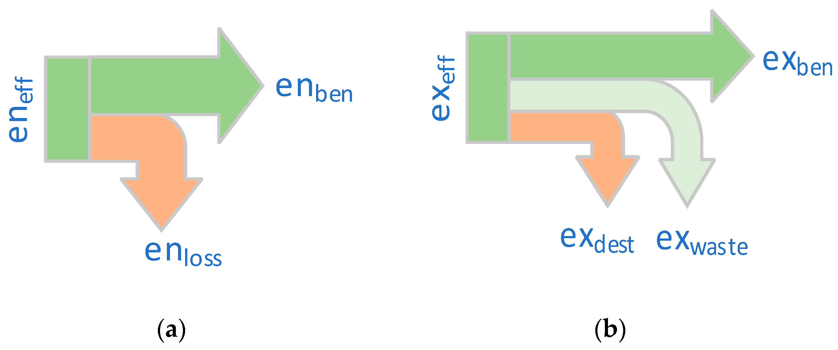
2.1.4. Energy and Exergy Efficiency

Technical processes and energy systems can be assessed based on their energy and exergy efficiencies. The energy efficiency η is defined as the ratio of energetic benefit $e{n}_{\mathrm{ben}}$ to energetic effort $e{n}_{\mathrm{eff}}$, as in Equation (6) and Figure 3. Similar to this definition, the exergy efficiency ζ is defined as the ratio of exergetic benefit $e{x}_{\mathrm{ben}}$ to exergetic effort $e{x}_{\mathrm{eff}}$, as shown in Equation (7).

$$\eta =\frac{e{n}_{\mathrm{ben}}}{e{n}_{\mathrm{eff}}}=1-\left[\frac{e{n}_{\mathrm{loss}}}{e{n}_{\mathrm{eff}}}\right]$$

(6)

$$\zeta =\frac{e{x}_{\mathrm{ben}}}{e{x}_{\mathrm{eff}}}=1-\left[\frac{e{x}_{\mathrm{waste}}+e{x}_{\mathrm{dest}}}{e{x}_{\mathrm{eff}}}\right]=1-\left[\frac{e{x}_{\mathrm{loss}}}{e{x}_{\mathrm{eff}}}\right]$$

(7)

Both equations can be illustrated as the ratio of loss to input. For exergy, a distinction has to be made between exergy waste $e{x}_{\mathrm{waste}}$ and exergy destruction $e{x}_{\mathrm{dest}}$:

• Exergy destruction describes the irreversible transformation from exergy into anergy during a process such as providing low temperature heat from a highly exergetic energy carrier such as natural gas.
• Exergy waste is the unused share of exergy in a discharged waste energy flow, such as exhaust gas of an internal combustion engine.

Exergy destruction and exergy waste are summarized in the exergetic losses $e{x}_{\mathrm{loss}}$. The exergetic benefit is defined as the exergetic effort less the exergetic losses $e{x}_{\mathrm{loss}}$.

Energetic efficiency is a process-dependent ratio of energy benefit to energy effort. Energy sources of different qualities are, following the first law of thermodynamics, mixed without distinction. In contrast to exergetic efficiency, it does not quantify energy degradation (Figure 3). Energy efficiencies also do not allow conclusions to be drawn regarding possible improvements for the process considered. For example, an adiabatic gas boiler transforms chemical energy into thermal energy with an energy efficiency close to η = 1. Due to the inevitable exergy destruction during the transformation from chemical to thermal energy, the exergy efficiency is ζ ≪ 1. This indicates that high-quality energy is transformed into a low-quality energy form during the process. When exergy is transformed into anergy, usable energy is lost. If additional heat losses to the surrounding environment, for example through hot exhaust gases, are considered, this part of the thermal exergy would be lost to the environment and become exergy waste. Briefly summarized, the exergy efficiency ζ clearly displays how closely a process operates to the theoretical, reversible optimum. In general, this is not true for the energetic efficiency [7].

Exergy and anergy flows can be calculated on the basis of energy flows, reference conditions of the environment, and technical processes of the considered energy system. Subsequently, exergy waste and exergy destruction can be calculated for every conversion step of all energy system elements. This quantitative evaluation approach can help to identify potential improvements when it comes to reducing the primary energy and fossil fuel demand. Additionally, the best energy carrier can be selected if the quality of the needed energy form is taken into account. Thus, the exergy efficiency of energy supply paths can be improved. Exergy waste is an indicator of potential environmental influences. Every exergy waste flow is able to alter the environment [9], but it can also be used to cover the exergy demand of other processes. Such cascaded energy systems can help to reduce the total exergy demand and increase the exergetic efficiency. Additionally, exergy analysis allows for the qualitative comparability of different technologies.

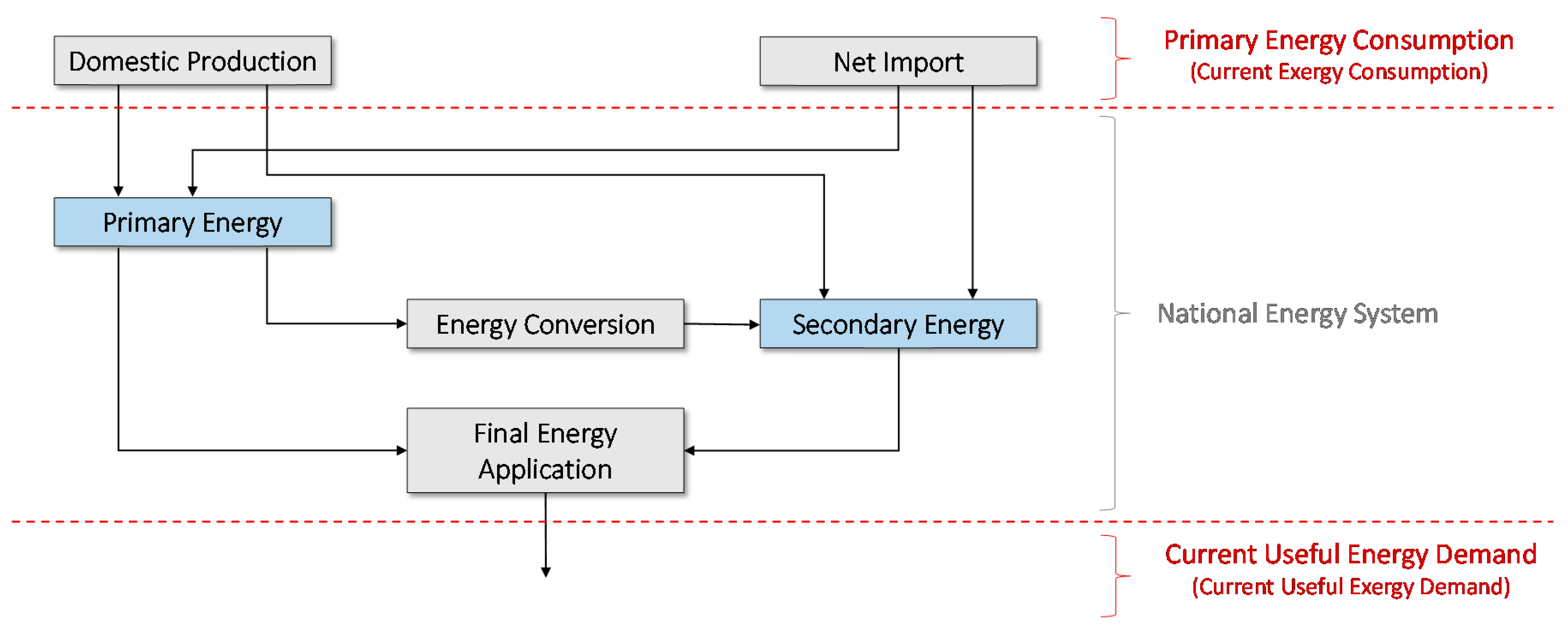
2.2. Definitions of Primary, Secondary and Final Energy

Primary energy carriers are energy carriers that can be found as natural resources, such as coal, crude oil or natural gas. They can be converted into secondary energy carriers through conversion processes, e.g., to simplify transport or utilization. Secondary energy carriers can only be provided by conversion. Examples for secondary energy carriers might be electricity, hydrogen, district heating, gasoline or diesel. Since conversion processes always cause losses, the secondary energy output is always lower than the primary energy input [13].

Final energy is the energy that is actually used by the final consumer, which means that in contrast to primary and secondary energy, transport and distribution losses are also taken into account. Therefore, it is equal to primary energy minus conversion losses and minus transport and distribution losses [14].

In accordance with International Energy Agency (IEA) guidelines, renewable energy carriers are in some cases classified as primary energy carriers (e.g., woody biomass) and in other cases as secondary energy carriers (e.g., electricity from photovoltaic systems or wind power plants). The first practically multiple usable energy carrier is always chosen. [15]

2.3. Definitions of Energy Consumption and Energy Supply

Some specific terms and definitions are necessary for describing the energy system on a national level, as it is considered in this work. In this section, the most important terms will be defined (according to the definition used by Statistics Austria [16]):

The Gross Inland Consumption (GIC) is the sum of the Indigenous Production of Primary Fuels (IP), the difference between Import (Imp) and Export (Exp), as well as the Stock Change (ΔStock). The GIC, which is also called the Total Energy Supply, describes the total nationwide energy consumption (Equation (8)).

$$GIC=IP+Imp-Exp\pm \Delta Stock$$

(8)

In contrast to Equation (8), which defines the GIC based on the energy supply, the GIC can also be calculated based on the energy consumption. This is the sum of the Consumption of Energy Sector Use (CES), the Transport Losses (TL), the Non Energy Use (NEU), the Final Energy Consumption (FEC) and the Transformation Input (TI) minus the Transformation Output (TO) (Equation (9)).

$$GIC=CES+TL+NEU+FEC+TI-TO$$

(9)

For clarification, the difference between the transformation output and input is the sum of all energy conversion losses. Fuels used as materials input, e.g., in the chemical industry, are labeled as non energy use. In addition, the CES defines the energy demand, required for the supply of secondary energy (e.g., the electrical energy demand of power plants).

The imports and exports consider primary as well as secondary energy. Therefore, by combining Equations (8) and (9), it can be determined that the GIC only takes conversion losses into account, which are within the system boundaries. This corresponds to the IEA specification [14] and must be taken into account when creating energy balance statistics in order to avoid double accounting. For example, country A imports electricity from country B, which uses a coal-fired power plant to generate electricity. In this example, the energy losses of the electricity generation are only included in the energy balance statistic of country B, even though the electricity is consumed by country A.

In comparison to the GIC, the primary energy consumption (PEC) does not include the NEU (Equation (10)) [17]. Therefore, the PEC describes the total energy used for energy purposes. According to the IEA guidelines [13,14], it includes primary energy production as well as net imported primary and secondary energy.

$$PEC=GIC-NEU$$

(10)

3. State of Research

In this section, a brief overview of published studies relevant for this paper is presented. For each of the three exergy amounts of Figure 1, a spatial separation as well as an exergetic assessment of the energy must be performed (Figure 4). Therefore, the exergetic assessment of energy systems is discussed in Section 3.1. Furthermore, in Section 3.2, a short overview of the possibilities of spatial separation of energy consumptions or potentials is given.

For methodological reference, Section 3.3 presents the different types of renewable potential studies. Furthermore, a selection of international and national studies is shown, and the different assumptions are discussed. The Austrian studies can also be used as a reference for the potentials calculated in this paper.

3.1. Exergetic Assessment

This section focuses on the exergetic assessment of energy systems. Therefore, a general overview is given in Section 3.1.1. As this paper addresses a large-scale system, selected case studies of such energy systems are discussed in Section 3.1.2. When determining the overall efficiency of large-scale systems, on the one hand the efficiency of the energy supply and on the other hand the efficiency of the final application have to be taken into account. Since the efficiency of the energy supply can easily be calculated based on published statistical data, the relevant exergy efficiencies of final energy applications are presented in Section 3.1.3.

3.1.1. Exergy Analysis: An Overview

Exergy analyses have been a field of special interest for more than 30 years now. Since exergy itself not only is a measure of quantity but also of quality [7,18], additional information can be obtained with exergy analysis. Dincer and Rosen [7] state that because these methods of analysis aim to detect energy inefficiencies, they allow for a much better identification of the causes and locations of energy losses (Section 2.1). Due to these and other advantages compared to the sole execution of energy analyses, exergy analysis is used in many different research areas:

Extensive information on different fields of application can be found, for example, in Dincer and Rosen [7]. According to [7], exergy analysis can be used, for instance, in fields like policy development, large-scale systems like countries, or application processes (e.g., heat pumps, cogeneration or renewable energy systems). The authors also presented the field of exergoeconomics, a combination of economic and exergy analysis, which can be used for both micro- and macroeconomic analyses [7].

For combining economic and exergy analysis, various approaches are available. These also include non-exergetic expenditure (e.g., labor, finance, environment), such as the concept of Extended Exergy Accounting (EEA) introduced by Sciubba [19]. This reference stated that exergy has an intrinsic, strong and direct correlation to economic values [19]. Another approach which combines exergy and economy, is the concept of exergetic costs by Lozano and Valero [20]. The cumulative exergy consumption (CExC) method, introduced by Szargut and Morris [21], describes how much exergy in total was needed to provide a product or a service [22]. Lazzaretto and Tsatsaronis [23] presented the specific exergy costing (SPECO) method that clearly defines the fuel and product of system components. They compared their approach to other concepts. A more detailed bibliography for different methods in this field can be found in Sciubba and Ulgiati [24], Sciubba et al. [25] or Sciubba and Wall [26].

Besides technical and economic analysis and aspects, Dewulf et al. [27] noted that exergy analyses are used for many other areas. They stated that especially environmental impact analysis is one of the most mature fields of application when talking about Environmental Science and Technology. Additionally, Szargut [28] described applications in the field of ecology (e.g., exergy losses of living organisms) as promising, which was proven by the work of authors like Jørgensen, Nielsen and Bastianoni (e.g., [18,29,30]), whereas an application to social sciences can be considered unsuitable for the concept.

After this general overview of the wide range of applications of exergy analysis, large-scale systems such as countries will be discussed in detail in the following section, since this paper focuses on such a system.

3.1.2. Exergy Analysis of Large-Scale Energy Systems

To perform exergy analysis on large-scale systems, it is useful to consider them as thermodynamic systems because that allows the application of mass- and energy conservation [25]. Based on this assumption, exergy analysis has been performed for different large-scale systems. Exergy analysis of systems like countries, regions or sectors allows the identification of areas for large improvements regarding exergy efficiency [7]. [7] noted that these analyses provide insights into the efficiency of a society’s use of resources as well as information to balance economic aspects and efficiency issues.

When comparing studies, differences with regard to the system boundaries but also to the considered variables can be identified. Another difference lies in the intended outputs. Some examples of different system boundaries and methods are mentioned in the following:

• Ertesvåg [31] identified two main basic calculation approaches for exergy analysis of countries: Reistad’s approach [32] and Wall’s approach [33]. To receive exergy efficiencies, Reistad only took the flows of energy carriers for energy use into account, whereas Wall also considered material flows (e.g., wood, ores).
• Some studies considered useful exergy as beneficial (e.g., [7,34,35]), whereas others aimed to present the amount of the production output instead (e.g., [18]).
• EEA depicts the society in its entirety and does include non-material or energy-based aspects, such as capital, labor and environment [25].
• CExC is a resource-to-end-use calculation method and analyses the whole production line starting with raw materials and ending with the finished product or service. CExC results therefore present the total exergy consumption caused by the production process [21,22].

Although they all follow the basic principle of exergy theory, it is hard to compare results due to further specifications regarding the exact research interest. A short overview of research in the field of exergy analysis of large-scale systems is given in the current section.

Reistad’s famous exergy analysis of the United States of America in the 1970s seems to be the first analysis of a country considered as a large-scale system. Since then, many other countries and regions, as well as sectors, have been analyzed. A comprehensive comparison of exergy efficiency studies for more than 10 countries was performed by Ertesvåg [31]. He concluded that the exergy efficiencies of final applications range between 20% and 30% and the total exergy efficiencies for the countries analyzed (e.g., Norway, Canada, USA) range between 9% and 28%.

Utlu and Hepbasli [36] also compared different studies (some of which were also part of the analysis done by [31]) for various years and determined the total exergy efficiency of the considered countries to be between 15% and 39%. In contrast to the exergy efficiency of final applications, the total exergy efficiency takes the whole energy system into account, including both losses of the energy supply and losses of the final application.

Utlu and Hepbasli [37] used an approach proposed by Rosen and Dincer [38], which is very similar to Reistad’s approach, in order to calculate exergy efficiencies for four sectors (utility, industry, transport, commercial and residential sector) of Turkey for 1999 and 2000. The efficiencies range between 8% (commercial and residential sector in 2000) and 36% (transport in 1999).

Nielsen and Jørgensen [39] conducted a sustainability analysis based on exergy analysis for different sectors of the Danish island Samsø. They implemented a hierarchical and geographical based system and methodology. Skytt et al. [40] adapted the method of [39] and applied it to the larger scale system of Jämtland in Sweden and additionally included further considerations about the application of material flows.

A study performed by Koroneus et al. [41] about energy and exergy utilization in Greece for the residential and industrial sectors in 2003 showed exergy efficiencies of 21% (residential sector) and 51% (industrial sector).

Rosen [42] dealt in particular with efficiencies in the industrial sector. To perform the evaluation, he analyzed each industry sector (e.g., iron and steel, construction) separately. Then, he combined them to get the overall industrial exergy efficiency. The global industrial exergy efficiency is proposed as 30%.

Lindner et al. [9] conducted an exergy analysis for Germany and came to the conclusion that energy carriers with a high exergy content, such as oil or gas, are used for fundamentally wrong purposes. This caused a total exergy efficiency of only 18% in Germany.

A similarly low total exergy efficiency of 21% can be found in Gutschi et al. [3]. This study dealt with exergy flows in Austria in 1956 and 2005. The highest exergy destruction occurs in space heating applications, where energy carriers with high exergy content (e.g., gas) are used to provide heat on a low temperature level. The usage of heat pumps or of combined heat and power plants would be better.

Other studies also included financial aspects in their considerations. These extended exergy accounting analyses can also be used on national or regional scales, as seen in Sciubba et al. [25] for the case of Siena or Ertesvåg [43] for Norwegian society.

All these exergy efficiency key figures support one central point—that the current energy systems lack efficiency in the use of exergy and therefore offer enormous potential for optimization and savings.

3.1.3. Exergy Efficiency of Final Energy Applications

In order to calculate the useful exergy demand from the useful energy demand, the exergy efficiencies of final energy applications are necessary. For the Austrian road traffic sector, the exergy efficiencies of the vehicle pool based on distance driven per vehicle category have been calculated. The average exergy efficiency of the Austrian internal combustion engine (ICE) vehicle pool in 2018 was 27% when transforming final energy to the useful energy form of traction. Only the traction energy is defined as a benefit. In that case, energy and exergy efficiencies are equal. If all vehicles fulfilled the newest emission standards, the efficiency would increase only slightly to 29%. The exergetic efficiency of vehicles could be substantially improved if electric mobility such as battery electric vehicles and fuel cell vehicles are used. These values are provided by the Institute of Internal Combustion Engines and Thermodynamics (Graz University of Technology) and HyCentA (publication in process).

The efficiencies of other final energy applications and gas transport are listed in

Table 3. Exergy and energy efficiencies of other final energy applications.

Technology	Exergy and Energy Efficiency ζ = η in %
Railway 1—Diesel	28 2–30 3
Railway 1—Electric	65 2–85 3
Aircraft [7]	20–28
Ship—Diesel	15–30
Stationary Electric Motor Systems [45]	50
Stationary Diesel/Gas Engines [47]	42–50
Lighting—Halogen [48]	12–15
Lighting—Fluorescent Lamp T5 [48]	24
Lighting—LED [48]	42–49

¹ Efficiencies have been calculated with a longitudinal dynamics model by HyCentA, ² With interior heating, ³ Without interior heating.

. The efficiency of diesel trains in Austria can be indicated by 28% to 30%. In general, light-emitting diode (LED) lamps can reduce the final energy and exergy consumption by substituting light bulbs. Based on the efficiency of stationary diesel engines and a propulsion efficiency of 40%–65% [44], the efficiency of ships is stated as 15%–30%. The theoretical efficiency of electrical stationary engines of over 90% is not attained. According to [45], the mean electric motor efficiency is currently 79%. Due to losses in components such as gears, breaks, valves and control units the efficiency of electric motor applications can be as low as 20%–40% [46]. On average, the efficiency of stationary electric motor applications is 50% and can be further improved by 20%–30% [45].

While discussing the efficiency of final energy applications, long-distance gas pipelines must also be considered, according to the definition of Statistics Austria [49]. The long-distance pipelines are primarily used for supra-regional and international gas trading and not for domestic supply. When the gas in the pipeline is used to fuel the gas compressor station, the compressor efficiency of 75%–84% and the efficiency of the gas turbine used to operate the compressor of 28–35% have to be taken into account [50]. Gas compressor stations typically use less than 1% of the transported gas to power the compressors [51].

3.2. Spatially Resolved Energy Modelling (Top-Down and Bottom-Up)

Two basic modeling approaches are generally used in the field of spatial energy modeling: top-down and bottom-up. Depending on the available data and purpose, it is necessary to choose one, although, a hybrid approach with a combination of both might also be reasonable. Bottom-up analysis uses disaggregated data that are later aggregated and extrapolated to obtain results. The top-down analysis relies on aggregated data which are then split up for the task at hand [52,53]. These modeling techniques are therefore methodologies in a reverse direction [54]. Other widely used modeling techniques are based on Index Decomposition Analysis (IDA) methods. By first defining a governing function, it is possible to connect the aggregate to be decomposed to pre-defined factors of interest and then quantify the component’s effect on the system [55]. According to Fengling’s [54] study about decomposition analysis’ application to energy, these methods can also be considered as top-down approaches.

Bottom-up approaches, like statistical analysis (e.g., linear regression), can be used for predicting residential energy consumption as was shown by Fumo and Rafe Biswas [56]. They stated that, according to a literature review, regression analysis is feasible for model development in this sector. Kazemi et al. [57] also used a regression model for the forecasting of the industrial energy demand of Iran. Scarlat et al. [58] performed a spatial analysis of biogas potential from manure in Europe following a bottom-up approach by aggregating the manure produced by all livestock units in a spatial unit.

Angelis-Dimakis et al. [59] analyzed different top-down methods to evaluate the availability of renewable energy sources, such as wind and solar resource potentials. The authors remarked that, especially for RES, a strong geospatial connection prevails. In the study of Fleiter et al. [60], researching barriers of energy demand models, the authors claimed that top-down models often represent economist’s viewpoints whereas bottom-up models follow technological pathways. Top-down models are therefore suitable for the modeling of interactions between energy systems and economic variables. As discussed in Koopmans and te Velde [61], top-down models propose lower energy efficiency and higher energy demand than bottom-up models. Due to that, hybrid approaches are a reasonable alternative.

Li et al. [62] discussed model techniques of urban building energy use. As seen in other publications, they distinguished top-down and bottom-up approaches that are both used in combination with Geographical Information Systems (GIS). Abart-Heriszt et al. [5] linked bottom-up and top-down methods to perform a spatially differentiated analysis of final energy consumption patterns and associated greenhouse gas emissions on a municipal level in Austria. Ramachandra and Shruti [63] also applied top-down and bottom-up techniques for the spatial mapping of renewable energy potentials in Karnataka, India.

The results of the modeling approaches presented in this section can be used for geospatial applications and visualization afterward. Therefore, the spatial units have to be chosen individually for each case, depending on the modeling approach and data availability. Depending on the available data, it is possible to transform these models to different scales such as regional or national.

3.3. Potential of Renewable Energy Sources (RES)

In principle, a distinction can be made between the theoretical potential, the technical potential, and the reduced technical potential.

The theoretical potential is described by the physical supply within a certain scope. It represents the upper physical boundary and does not consider ecological, economic, social, structural or administrative aspects. For example, the theoretical biogas potential for Germany is defined as the proposed maximum methane yield per hectare multiplied by the area of Germany [64].

The technical potential is based on the theoretical potential but considers state of the art technologies and is reduced by the actual structures of the society (e.g., building and road infrastructures, the amount and composition of waste or the amount of livestock). There is no consideration of changes in the current structures (e.g., changes in land use), of economic aspects, of different paths of utilization, of feasibility or of social aspects.

The reduced technical potential or the economic–technical potential can be calculated by taking additional criteria such as political conditions, different utilization pathways or economic aspects into account.

3.3.1. International RES Potential Studies

Potentials of RES are published in numerous international studies and vary greatly in their values. Most of these studies present data on technical potentials for different energy carriers such as solar energy, wind energy, hydro energy, biomass, geothermal energy and ocean energy.

IPCC [65] presents the technical potentials of six different renewable energy carriers. In contrast to other studies, biomass and solar energy are presented as primary energy because of its diverse forms of use. The total worldwide potential ranges between 1895 and 52,802 EJ/a (about 526 to 14,667 PWh/a). Rogner et al. [66] show a total technical potential between 67,510 and 294,625 EJ/a (about 18,753 to 81,840 PWh/a) for the same energy carriers as [65].

Many studies also offer country- or state-level data. However, due to scale and a multitude of assumptions, there are enormous differences between various studies, and it is hard to compare the results in detail.

Exergetic analysis itself is only performed for different RES applications such as solar energy like seen in Saidur et al. [67], Park et al. [68] or Svirezhev [69]. No studies on spatially resolved exergy potentials that operate nationwide on district level could be found.

3.3.2. RES Potential Studies in Austria

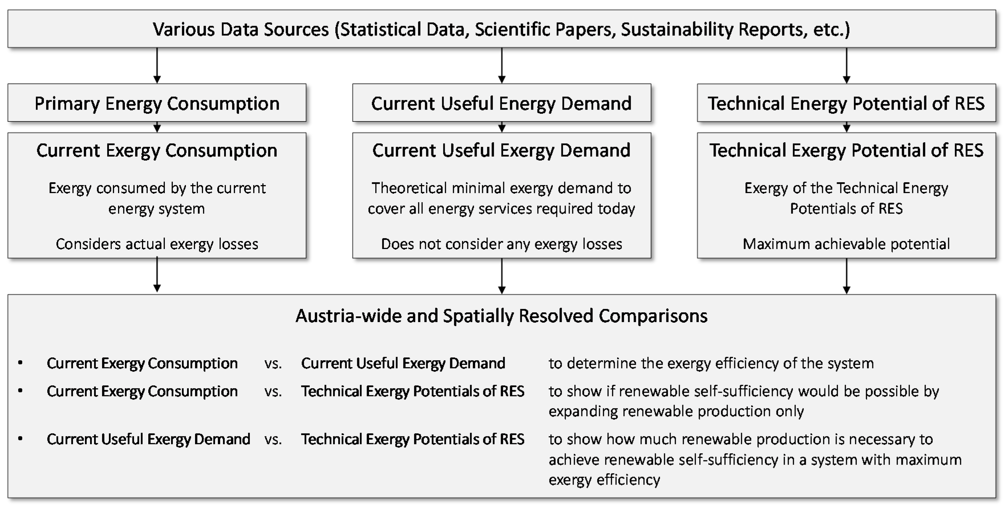
There are a few different RES potentials studies available for Austria (

Table 4. Austrian RES potential studies.

	Technical Potential in TWh/a	Reduced Technical Potential in TWh/a	Economic-Technical Potential in TWh/a
Stanzer et al. [6]	607	357	−
Kaltschmitt and Streicher [70]	266 to 536	−	−
Winkelmeier et al. [71] 1	51	−
Pöyry [72] 2	75	−	56
Moser, Sejkora et al. [4]	−	219	−
Brauner [73]	−	−	100

¹ only wind power energy potentials are analyzed, ² only hydro power energy potentials are analyzed.

). These studies vary in type (technical, reduced technical or economic-technical potential), in the energy carriers taken into account (e.g., geothermal energy, ambient heat, photovoltaics or solar thermal energy (ST)) and in their assumptions. Stanzer et al. [6] published data on technical potentials. Kaltschmitt and Streicher [70] introduced the terms of technical supply potential and technical demand potential. According to their definitions, supply potentials can be compared to technical potentials as used in [6]. [6] and Moser, Sejkora et al. [4] published reduced technical potentials (Table 4).

Some studies only focused on potentials for one renewable energy carrier such as Pöyry [72] on hydro power energy potentials or Winkelmeier et al. [71] on wind power energy potentials. The maximum of attainable wind potential, which was calculated by Winkelmeier et al. [71], can be compared to technical potentials. Pöyry [72] released data on technical and economic-technical potentials of hydro power. The results of [72] were also used as a reference in other studies mentioned (e.g., [70]).

As this work is based on technical potentials, only these are discussed in the following section. Depending on differences in technical assumptions (e.g., different collector types), Kaltschmitt and Streicher [70] calculated different technical potentials for PV, ST and ambient heat, which led to a large value range in total RES potentials of 266 to 536 TWh/a. Since multiple variants for the use of RES are possible (e.g., ST collectors vs. PV collectors on the same area, ST/PV collectors vs. areas for biomass on currently unused land) the term competition of energy technologies is introduced. Therefore, they published two versions of the data, one of which also considers competition between different energy technologies. The value deviation between these versions is about 10%. Stanzer et al. [6] published a total RES potential of 607 TWh/a. They did consider competition for area between energetic and non-energetic forms of use (e.g., use of arable land for biomass or food and feed production) but did not take into account competition of energy technologies (e.g., ST vs. PV).

There is a big range of the potentials presented because the technologies (e.g., collector types) considered and the assumptions regarding areas for renewable energy generation (exploitable areas) vary.

4. Methodology

In general, the goal of any national energy system is the provision of useful energy (e.g., mechanical work, heat) to meet human needs (e.g., movement, comfortable room temperature). To satisfy these energy service needs, each final energy application consumes final energy to provide useful energy. The final energy consumption can be covered by the utilization of primary or secondary energy carriers. As mentioned before (Section 2.2), primary energy carriers are those energy carriers that can be found as natural resources (e.g., coal) whereas secondary energy carriers (e.g., electricity) are provided by the conversion of primary energy carriers. Internal losses occur when converting primary energy carriers to secondary energy carriers, during transport to the final energy application and in the final energy application itself (Figure 5).

In this paper, a national energy system is analyzed. First, the system boundaries must be specified, as shown in Figure 5. Accordingly, the energy flows into and out of the national energy system are determined first and evaluated exergetically afterward.

On the basis of a national energy system, as shown in Figure 5, three exergy amounts can be determined. For this purpose, the inputs on the one hand and the outputs of the energy system on the other hand are analyzed. These three quantities are determined and then compared with each other in order to make statements about the analyzed energy system:

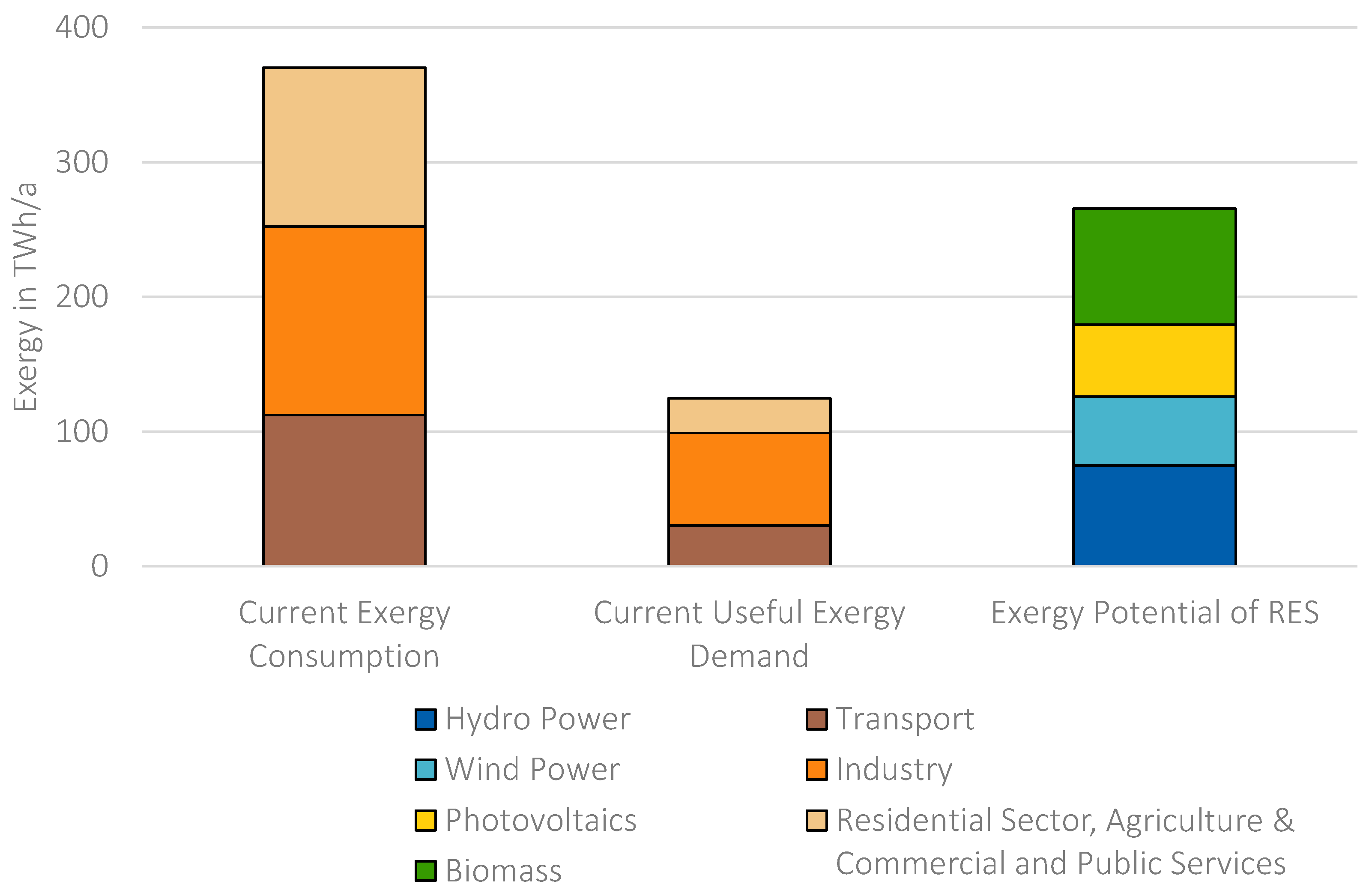
• Current exergy consumption. First, the total of energy that flows into the system is considered. This takes all energy for energy purposes which is used directly (without conversion processes) or indirectly (with conversion processes) by the energy system into account, including all mentioned internal losses. The energy that flows into the system is defined as primary energy consumption [14,49] (Figure 5). According to the IEA guidelines, the primary energy consumption of one country is the sum of domestic primary energy production (e.g., oil extraction, woody biomass production), domestic secondary energy production (e.g., electricity from photovoltaics), net imported (net import describes the difference between import and export) primary energy (e.g., sectors natural gas import) and net imported secondary energy (e.g., electricity import). In addition, stock changes of primary and secondary energy are also included. [13,14]. The primary energy consumption is used to determine the current exergy consumption, which is the first of the three exergy amounts.
• Current useful exergy demand. Next, the flow of useful energy out of the national energy system is balanced (Figure 5). It is the second of the three exergy amounts of this paper. The result of the exergetic analysis of the useful energy is called current useful exergy demand. It describes how much exergy is actually necessary to satisfy all energy service needs of one country. An energy service, and therefore the current useful exergy demand, is technology independent. An example is the provision of hot water, which can be provided by a heat pump or by a gas boiler.
• Technical exergy potentials of RES. Domestic production also includes the generation of local RES. This will play an important role in future national energy systems (e.g., [74]). Therefore, in addition to the analysis of the energy and exergy consumption of the current energy system, this paper also considers the technical potentials of RES. This can also be seen as an energy flow into the system. The exergetic analysis of the technical potentials of RES results in the third of the three exergy amounts of this paper. It indicates the maximum of exergy, which can be generated per year in a certain area, using the latest available technologies and without changing any structures such as land use. Other aspects such as economic efficiency, different paths of utilization, feasibility or social aspects are not considered.

According to the IEA guidelines, this paper considers the potentials of RES in the first multiple usable energy carrier. Therefore, some renewable energy sources are considered primary energy (e.g., woody biomass) and others secondary energy (e.g., electricity from photovoltaics, biogas from sewage sludge). The technical potentials of RES are first energetically calculated and afterward exergetically assessed in order to determine a technical exergy potential of RES of one country.

As mentioned in the introduction, first, the three basic exergy amounts are explained and determined in detail: current exergy consumption (Section 4.1 and Section 4.2, since the current exergy consumption is based on primary energy consumption, which is explained in Section 4.1), current useful exergy demand (Section 4.3) and the technical exergy potentials of RES (Section 4.4). Then, these three exergy amounts are compared to each other in the results section to obtain the following findings (Figure 6):

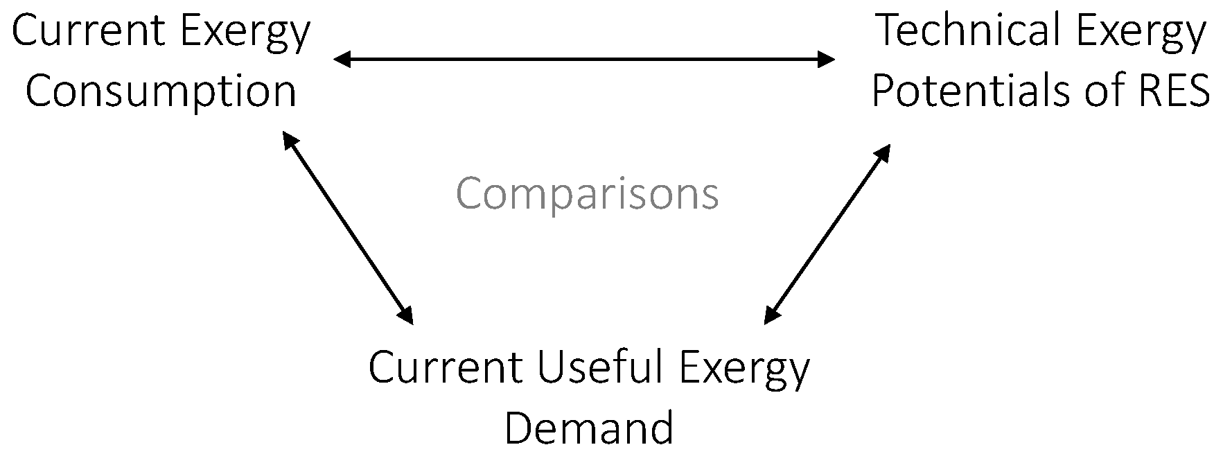
• Comparison of current exergy consumption and the current useful exergy demand to determine the exergetic efficiency of the currently used energy system
• Comparison of current exergy consumption and the technical exergy potential of RES to show if renewable self-sufficiency is possible by expanding renewable production only
• Comparison of the current useful exergy demand and the technical exergy potential of RES to show how much renewable production is necessary to achieve renewable self-sufficiency in a system with maximum exergy efficiency.

The methodology of this work is explained using the example of Austria. Thus, this study presents a comprehensive analysis of the situation in Austria. All comparisons are carried out Austria-wide and spatially resolved. Therefore, in addition to overall statements about Austria, spatially resolved conclusions such as the under- or over-coverage of one individual district can be made. Section 4.5 shows how this methodology and therefore the whole analysis can also be adapted for other countries while the results of all comparisons are shown and discussed in the Section 5 and Section 6.

4.1. Spatially Resolved Primary Energy Consumption

In order to enable a comprehensive description and analysis of the Austrian energy system, the PEC was used as the basis for the determination of the first of three exergy amounts: the current exergy consumption.

The definition of the PEC includes all losses (e.g., conversion losses, transport losses) which take place within the national energy system. Therefore, all losses that do not take place within the national energy system e.g., due to imports of secondary energy, are consequently excluded (Section 2.3). [14,17]

In order to enable a spatial segmentation, the PEC needs to be divided into different sectors, such as industry, transport, residential, and others. It must be mentioned that most sectors consume both primary energy (e.g., coal) and secondary energy (e.g., district heating or electricity). Therefore, the conversion losses of energy supply, which occur when providing secondary energy, the transport losses as well as the energy consumption for providing energy (e.g., on-site power of power plants) must be allocated to their respective sector. This allocation is performed according to their amount of energy consumption. Thus, this approach is comparable with the “polluter pays” principle in the field of environmental protection. In this paper, this Proportionally Allocated Consumption of the Energy Supply (PACS) only considered public infrastructure losses since the transformation losses (transformation input TI minus transformation output TO) of industrial conversion units such as company-owned plants (provision of heat and electricity), refineries (conversion of crude oil to various products), coke ovens (conversion of coal to coke) and blast furnaces (conversion of coke to blast furnace gas) are assigned to the corresponding industrial subsector directly. Most of these industrial transformation losses also have a corresponding industrial consumption of energy sector use (CES). The CES describes the energy consumption, which is necessary to enable the conversion process (e.g., the energy to run the coke oven at the necessary temperature).

Therefore, the primary energy consumption of the sector s can be expressed according to Equations (9)–(11). For each sector, it is the sum of the FEC, the CES, the transformation losses (TI-TO) and the PACS.

$$PE{C}_s=FE{C}_s+CE{S}_s+PAC{S}_s+T{I}_s-T{O}_s$$

(11)

PEC_s 

Primary energy consumption of sector s

FEC_s 

Final energy consumption of sector s

CES_s 

Consumption of energy sector use of sector s

PACS_s 

Proportionally allocated energy consumption of the energy supply for sector s

TI_s 

Transformation input of sector s

TO_s 

Transformation output of sector s

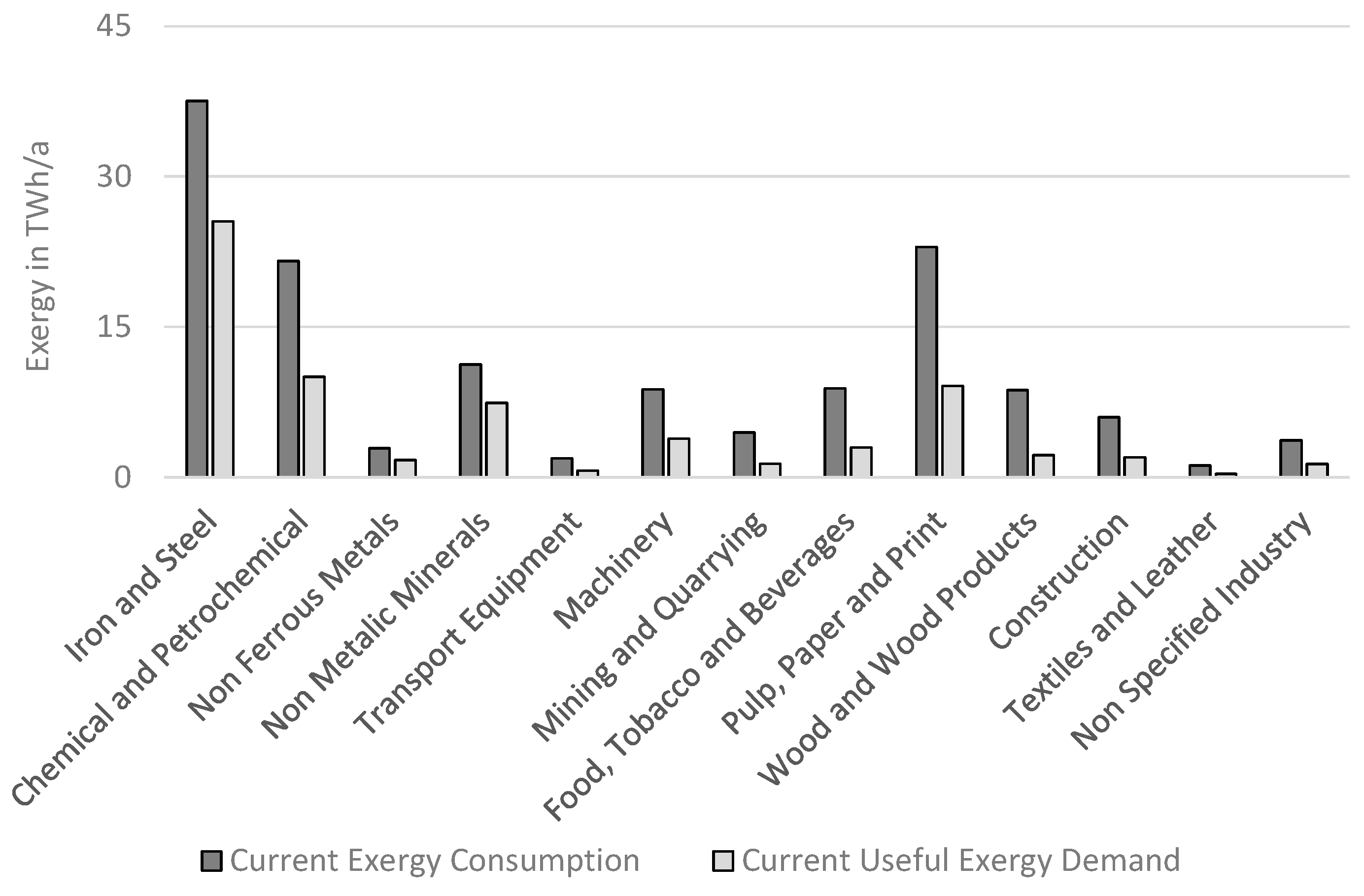
The spatial segmentation of the primary energy consumption was performed individually for each sector. In general, a similar segmentation method is used for the industry, residential, public and private services sectors as well as agriculture and is based on segmentation factors such as inhabitants or number of people working in one specific industrial subsector per district. In order to enable spatial segmentation, the transport sector needs, in addition to segmentation factors (e.g., number of registered vehicles per district), information about the transport infrastructure, such as the length of motorways or rails per district. Due to the granularity of published data, it is not possible to achieve a higher spatial resolution of the primary energy consumption than the Austrian district level. Therefore, the Austrian political districts of 2016 are used. The spatial segmentation of the primary energy consumption per sector will be discussed in detail in Section 4.1.1, Section 4.1.2 and Section 4.1.3.

4.1.1. Industry

The industrial primary energy consumption were calculated using Equation (11). For this, the industrial transformation loss, which is the difference between transformation input and output, (e.g., company-owned power plants), the consumption of energy sector use (e.g., the energy necessary to enable the transformation processes in a blast furnace or coke oven), the industrial final energy consumption as well as the proportionally allocated energy consumption of the energy supply (e.g., caused by electricity drawn from the public grid) were taken into account (

Table 5. Determination of the primary energy consumption for sector s = Industry, based on Equation (11).

Operator	Symbol	Explanation
+	$CE{S}_{Ind}$	Consumption of energy sector use (coke ovens, blast furnaces, oil refineries)
+	$FE{C}_{Ind}$	Final energy consumption in manufacturing industries and construction
+	$T{I}_{Ind}$	Transformation input (coke ovens; blast furnaces; refineries; charcoal production; company-owned power, heating, and combined heat and power (CHP) plants)
−	$T{O}_{Ind}$	Transformation output (coke ovens; blast furnaces; refineries; charcoal production; company-owned power, heating, and CHP plants)
+	$PAC{S}_{Ind}$	Proportionally allocated energy consumption of the energy supply
=	$PE{C}_{Ind}$	Industrial primary energy consumption

). The different terms of Equation (11) were determined using the energy balance statistics from Statistics Austria [2].

In order to enable the spatial separation of the industrial primary energy consumption, it was split into the different industrial subsectors (iron and steel, chemical and petrochemical, nonferrous metals, nonmetallic minerals, transport equipment, machinery, mining and quarrying, food, tobacco and beverages, pulp, paper and print, wood and wood products, construction, textiles and Leather, and non-specified industry. Classification by Statistics Austria [2]) in a first step. To perform this split, each mathematical term of Equation (11) and Table 5 was divided into different subsectors. A detailed breakdown of how this split was made can be found in Appendix A (

Table A1. This table shows, how the industrial subsector resolved primary energy consumption is calculated, based on energy balances, which are published e.g., by Statistics Austria [2,16]).

Industrial Subsector 1	Final Energy Consumption	Consumption of Energy Sector Use	Transformation Input	Transformation Output
Iron and steel	Final energy consumption of iron and steel	- Coke ovens - Blast furnaces	- Everything to coke ovens - Everything to blast furnaces - Coke oven gas, and blast furnaces gas to company-owned plants - Natural gas and Hydro power to company-owned plants	- Everything from coke ovens - Everything from blast furnaces - Electricity and district heating from company-owned plants
Chemical and petrochemical	Final energy consumption of chemical and petrochemical	- Oil refineries	- Everything to refineries Hard coal, oil products 2 natural gas, industrial waste, municipal waste (non-renewable), wood waste, biogas and other solid biofuels to company-owned plants	- Everything from refineries - Electricity and district heating from company-owned plants
Nonferrous metals	Final energy consumption of nonferrous metals	-	-	-
Nonmetallic minerals	Final energy consumption of nonmetallic minerals	-	-	-
Transport equipment	Final energy consumption of transport equipment	-	- Natural gas to company-owned plants	- Electricity and district heating from company-owned plants
Machinery	Final energy consumption of machinery	-	- Oil products 2 and natural gas to company-owned plants	- Electricity and district heating from company-owned plants
Mining and quarrying	Final energy consumption of mining and quarrying	-	-	-
Food, tobacco and beverages	Final energy consumption of food, tobacco and beverages	-	- Oil products 2, natural gas and biogas to company-owned plants	- Electricity and district heating from company-owned plants
Pulp, paper and print	Final energy consumption of pulp, paper and print	-	- Black liquor, hard coal, oil products 2, natural gas, industrial waste, municipal waste (non-renewable), wood waste, biogas, other solid biofuels, hydro power to company-owned plants	- Electricity and district heating from company-owned plants
Wood and wood products	Final energy consumption of wood and wood products	-	- Natural gas, wood waste, other solid biofuels to company-owned plants	- Electricity and district heating from company-owned plants
Construction	Final energy consumption of construction	-	-	-
Textiles and Leather	Final energy consumption of textiles and Leather	-	-	-
Non specified industry	Final energy consumption of non specified industry	-	- wood for charcoal production	charcoal

¹ Classification by Statistics Austria [2], ² Oil products are a combination of crude oil and Natural Gas Liquids (NGL), refinery feedstocks, gasoline, kerosene, diesel, gasoil, fuel oil, LPG, refinery gas as well as other oil products.

).

Using published energy balances statistics according to international IEA standards e.g., from Statistics Austria [2], this split was easy for most of the mathematical terms, since the final energy consumption is published for each subsector. Furthermore, coke ovens and blast furnaces are allocated to iron and steel, refineries to chemical and petrochemical as well as charcoal production to non specified industry. Only some transformation inputs and outputs of company-owned power, heating, and CHP plants are not obvious to allocate since transformation inputs and outputs are not published per subsector. However, some transformation inputs and outputs can be assigned by contextual considerations (e.g., utilization of blast furnace gas can be directly allocated to the iron and steel subsector or black liquor to the pulp, paper and print subsector), but not all. For example, the natural gas-fired company-owned CHP plants are used in several subsectors, such as iron and steel, chemical and petrochemical or food, tobacco and beverages. We were not able to allocate these and similar transformation inputs which are natural gas, industrial waste, non-renewable municipal waste, renewable municipal waste, landfill gas, sewage sludge gas, other biogas and hydro power (in total approx. 8% of all industrial transformation inputs). We estimated them based on a literature review, which had its focus on production processes and energy consumptions of Austrian companies. Therefore, all publicly available information, such as sustainability reports and statistics, were used, in order to make the allocation as reasonable as possible. All details for the calculation of the industrial subsector resolved energy consumption are given in Appendix A (Table A1). This table includes everything but PACS, since the allocation of PACS is performed proportional based on the total fossil consumption and the total electricity drawn from the public grid per industrial subsector from Table A1. Then, after also adding PACS, the subsector resolved industrial primary energy consumption was determined. Based on this, in the second step, a spatial separation was accomplished. Therefore, a combination of a bottom-up with a top-down approach was used:

First, all publicly available energy demand data of industrial sites was used in a bottom-up approach. These energy demands can be primarily found on companies’ websites as well as in their sustainability reports. Sustainability reports contain information on sustainable issues [75], such as waste treatment, energy consumption or accidents at work. Based on sustainability reports [76,77,78,79,80,81,82,83,84,85,86,87,88,89,90,91,92,93,94,95,96,97,98,99,100,101,102,103,104,105,106,107,108,109,110,111] the bottom-up based primary energy consumption for each industrial subsector and district was determined. With this approach, about 40% of the total industrial primary energy consumption was allocated, mostly for large industrial companies and their respective sites. Since these reports were published by the companies themselves, there are no statistical uncertainties and no errors in localization to be expected.

Next, the rest of the industrial primary energy consumption was allocated using a top-down approach. The fundamental assumption was that there is a linear relation between the primary energy consumption of the considered subsector and the respective numbers of employees. Based on the published employment data, the coefficient of this linear relation can be calculated for each industrial subsector and province of Austria. The combination of the corresponding coefficient and the numbers of employees was used to estimate the top down based primary energy consumption of one district (used data: [112]).

Finally, the sum of the bottom-up and the top-down based PEC was used to describe the total industrial PEC per district.

4.1.2. Residential Sector, Agriculture, and Commercial and Public Services

Determining the spatially resolved primary energy consumption of the residential sector, agriculture, as well as commercial and public services, is much easier than determining that of the industrial sector, since these three sectors all have no transformation input, no transformation output and no consumption of energy sector use. Therefore, the PEC for each of these three sectors is just the sum of the corresponding FEC plus the corresponding PACS (Equation (11)).

In this section, these three sectors are discussed combined, since the same methodology for calculating the spatial distribution of the PEC is used for all of them. This methodology is also similar to the top-down approach we used for the spatial segmentation of the industrial sector (Section 4.1.1). As explained in the previous section, the fundamental assumption for the two sectors, agriculture as well as commercial and public services, is a linear relation between the number of employees and PEC in one sector (used data: [2,112,113]). For the residual sector, the number of inhabitants and the residential PEC was used (used data: [114]). These assumptions enabled the determination of the PEC for the residential sector and agriculture, as well as commercial and public services per district in Austria.

4.1.3. Transport

The transport sector includes overland transport (primarily passenger cars and trucks), railways, inland navigation, aviation, and long-distance pipelines. The PEC of the transport sector is equal to the sum of FEC and PACS (Equation (11)). PACS must consider the relevant energy carriers per sector. In the transport sector, these are liquid fuels like gasoline, diesel or kerosene, but also electricity and natural gas. Since the conversion losses for the provision of liquid fuels are taking place in the refinery and the refinery is per definition allocated to the industry (Section 4.1.1), PACS in the transport sector only takes electricity as well as natural gas for long distance pipelines into account.

In this work, we tried to allocate the energy consumption of the transport sector to the location of its actual usage. Based on the published data alone, this was not always possible. Therefore, assumptions and simplifications were necessary:

The allocation of private passenger cars’ energy consumption was based on statistics about kilometres driven and fuel consumption of private cars by Statistics Austria [115]. There, the total final energy consumption of private cars is published per province. If it is assumed that private car traffic mainly takes place in the district in which the vehicle is registered, the final energy consumption can be split up between the different districts by the number of registered vehicles (used data: [116]). This assumption is based on the fact that the average mileage per private car in Austria is 31 km per day in 2017/2018 [115].

Trucks can be divided into two groups. On one side, there are trucks which are only used locally. These local trucks are only used for short distances, starting and stopping every day at the same point—34% of all distances driven during domestic transports are shorter than 50 km [117] This statistic includes only domestic transports which are operated by trucks registered in Austria [117]. This is justified as 99.3% of the total transport volume up to 49 km is carried out by trucks registered in Austria [118]. Through the total number of kilometres driven for short domestic transports (less than 50 km), which is available per province, and the average consumption of a truck (29.1 l Diesel per 100 km [119]), the total FEC of these local trucks can be estimated on a provincial level. It was assumed that the consumption of these local trucks primarily occurs where the truck is registered due to the short transport distances. Therefore, the spatial separation was based on the number of registered trucks per district [116].

The final energy consumption of the remaining overland transport was calculated by the difference between the total overland transport per province [113] and the already allocated consumption of private passenger cars and local trucks. This includes business passenger cars and trans-regional trucks and mainly takes place on motorways and expressways. In order to take this into account, a spatial separation was performed by the length of motorways and expressways per district. The length, as well as the position of the Austrian motorway and expressway infrastructure, was extracted from OpenStreetMap (OSM). OpenStreetMap is a collaborative project, which collects and structures geographic data, such as buildings, paths, streets, rivers or forests [120].

The methodology used for the spatial separation of the remaining overland transport was also used for railways, inland navigation and long-distance pipelines. Therefore, the final energy consumption per province for the mentioned applications [113] was spatially separated by the length of the rail infrastructure as well as by the length of the Danube. Only the Danube was taken into account, as it is the only international waterway in Austria which is relevant for the transport of goods [121,122]. The Danube is part of a European waterway which connects the North Sea with the Black Sea. The length of the rail infrastructure and the length of the Danube have both been extracted from OSM. The published data from GSV—Austrian Association for Transport and Infrastructure—were used for the length and position of the long-distance oil and natural gas pipelines [123].

For each of these considered applications, a specific FEC per kilometer of infrastructure or waterway was calculated. Thus, the FEC is distributed evenly rather than taking the actual average traffic load per km into account. This assumption had to be made since there are no traffic flow data of Austria published. However, based on the available data, at least a simplified weighting can be achieved. For example, important railway lines such as the Western Railway (“Westbahn”) in Austria usually have two or four parallel rails. Thus, in the calculation, these railway lines were weighted two or four times in comparison to a single-rail section of a side line. This principle was also applied to the calculation of the remaining overland transport based on the number of motorway and expressway lanes as well as to the calculation of the long-distance pipelines based on the number of parallel pipes.

Contrary to the principle of determining consumption where it actually occurs, the FECs of aviation were allocated to the airports, since there are no data available which would enable a spatial separation. The FECs are published for each province of Austria [113]. Since there is not more than one airport with considerable fuel consumption and well-known location per province, no calculations for the spatial separation are necessary.

In order to calculate PEC of the transport sector, we just added PACS proportionally to the FEC, based on the actual electricity and natural gas consumption.

4.2. Spatially Resolved Current Exergy Consumption

Based on the previously calculated spatially and sectorial resolved PEC, we calculated the first of the three exergy amounts, the current exergy consumption. This describes how much exergy is currently consumed in Austria per year, without considering any efficiencies or any possible improvements. Therefore, it represents the status quo. It can easily be calculated by multiplying the spatially resolved primary energy demand per energy carrier by the exergy factors per energy carrier (Section 2.1). For chemical energy carriers such as natural gas or gasoline, an exergy factor of 1 is assumed.

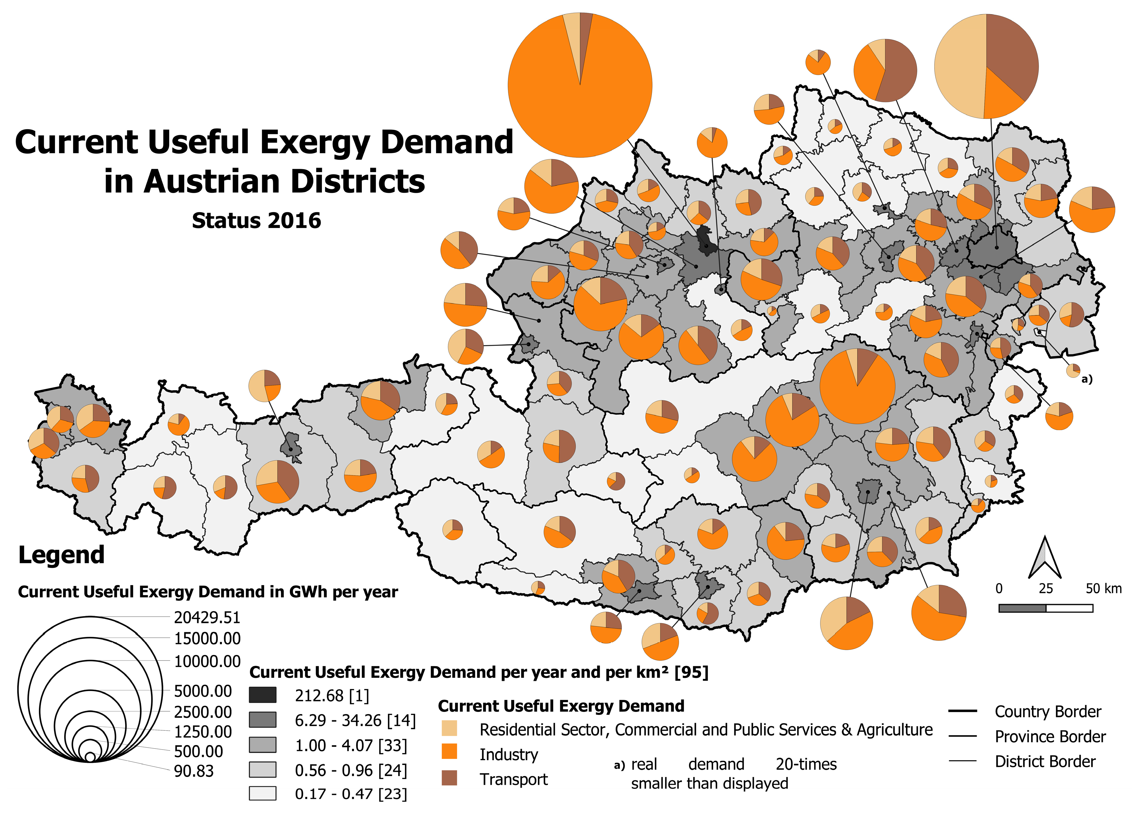
4.3. Spatially Resolved Current Useful Exergy Demand

In contrast to the current exergy consumption, the current useful exergy demand, which is the second of the three exergy amounts of this paper, does not take exergetic losses (e.g., conversion losses, transport losses, losses of the final energy application) into account. It is the exergetic assessment of the useful energy demand and describes how much exergy is actually needed to satisfy the energy service needs. Since it only describes how much exergy is needed, it is independent of the technology.

An example for such an energy service is the provision of hot water in residential buildings. Here, hot water is already the useful energy type. If we assume that the hot water service is provided by natural gas, the exergy consumption is nearly equal to the natural gas consumption, since the exergy factor of natural gas is approximately 1 (Section 2.1). However, the useful exergy demand is much lower than the exergy consumption. It can be calculated by multiplying the natural gas demand by the Carnot Factor, which is around 13%. The Carnot Factor is depending on the temperature of the hot water as well as the surrounding temperature. In this example a hot water temperature of 65 °C and a surrounding temperature of 20 °C is assumed.

Therefore, while the current exergy consumption is based on the primary energy consumption (Section 4.2) the current useful exergy demand is only based on the useful energy demand (Figure 5).

In addition to final energy applications, the useful energy demand must also include the CES (coke ovens, blast furnaces, oil refineries), since they consider the energy needed to run the corresponding processes (e.g., the blast furnace) [49]. The determination of the spatially resolved current useful exergy demand will be discussed for each sector in the following Sections (Section 4.3.1 and Section 4.3.2).

4.3.1. Industry, Residential Sector, Agriculture as well as Commercial and Public Services

As mentioned in the previous Section, only the final energy consumption, as well as the consumption of energy sector use, are used to determine the current useful exergy demand. Since in Section 4.1.1 and Section 4.1.2 each term of Equation (11) has been determined for each sector, the calculation of the spatially resolved current useful exergy demand was performed directly on these data. Furthermore, the useful energy analysis, provided by Statistics Austria [113] includes additional information about the applications of the energy use, e.g., for industrial furnaces, for stationary engines or for lighting, and information and communications technology (ICT). In this section, the current useful exergy demand is always calculated with the useful energy multiplied by the exergetic efficiency of the process. The required exergetic efficiencies can be found in Section 3.1.3. If an efficiency range instead of a single value is specified, the mean value is taken.

To determine the current useful exergy demand, a basic distinction must be made between heating and cooling applications (space heating and air condition, vapor production as well as industrial furnaces), stationary engines as well as electricity for lighting, ICT and electrochemical purposes.

The exergetic assessment of heating and cooling application was based on the actual necessary temperature levels of the energy utilization. For this purpose, a breakdown (combination of [113,124,125]; commercial and public services as well as agriculture are estimated) was used which described how much of the process heat demand per sector (or industrial subsector) takes place at which temperature level (Appendix A

Table A2. Share of the different temperature levels for heat demand (without space heating) per sector (Source: [113,124,125]. Commercial and public services, as well as agriculture are estimated).

Industrial Subsector 1	Hot Water	<100 °C	100–200 °C	200–300 °C	300–500 °C	500–1000 °C	>1000 °C
Iron and steel	0.1%	0.6%	0.9%	0.1%	0.7%	19.8%	77.8%
Chemical and petrochemical	0.2%	15.0%	10.5%	6.5%	6.1%	49.5%	12.2%
Nonferrous metals	0.1%	0.6%	0.9%	0.1%	0.7%	19.8%	77.8%
Nonmetalic minerals	0.1%	1.4%	1.2%	0.0%	0.8%	31.4%	65.1%
Transport equipment	10.6%	28.8%	11.5%	0.0%	8.7%	10.6%	29.8%
machinery	10.3%	27.6%	13.0%	0.0%	10.3%	10.8%	28.1%
Mining and quarrying	2.2%	1.4%	0.0%	0.0%	1.9%	30.8%	63.7%
Food, tobacco and beverages	1.1%	44.2%	51.3%	3.4%	0.0%	0.0%	0.0%
Pulp, paper and print	0.6%	18.6%	45.5%	1.9%	33.3%	0.0%	0.0%
Wood and wood products	0.0%	78.9%	10.5%	0.0%	10.5%	0.0%	0.0%
Construction	8.7%	8.4%	0.0%	0.0%	27.7%	17.8%	37.4%
Textiles and Leather	4.0%	96.0%	0.0%	0.0%	0.0%	0.0%	0.0%
Non Specified Industry	2.0%	22.0%	43.0%	2.0%	30.0%	0.0%	2.0%
Commercial and Public Services	0.0%	50.0%	50.0%	0.0%	0.0%	0.0%	0.0%
Residential Sector	84.9%	0.0%	15.1%	0.0%	0.0%	0.0%	0.0%
Agriculture	0.0%	50.0%	50.0%	0.0%	0.0%	0.0%	0.0%

¹ Classification by Statistics Austria [2].

and

Table A3. Assumed mean temperatures and Carnot Factor for the different heat applications and sources (surrounding temperature 10 °C).

Heat Demand or Source	Assumed Mean Temperature in °C	Carnot Factor in %
Ambient heat	10	0
Space heating	25	5
Hot water	65	16
Solar thermal energy	75	18
District heating	100	24
Process heat <100 °C	100	24
Process heat 100–200 °C	150	33
Process heat 200–300 °C	250	46
Process heat 300–500 °C	400	58
Process heat 500–1000 °C	750	72
Process heat >1000 °C	1500	84

). By multiplying these data by the (sub-) sector resolved total final energy demand of process heat (vapor production, industrial furnaces as well as the three industrial consumptions of energy sector use coke oven, blast furnace and refinery), the process heat demand per temperature level can be calculated for each sector and each industrial subsector. In addition to the process heat demand, the energy demand for space heating and air conditions per sector or per industrial subsector can directly be used, since it is published separately. The total exergy demand for heat and cooling applications per sector and per industrial subsector can be calculated by multiplying the energy demand per temperature level with their corresponding Carnot Factor (Appendix A Table A3).

The electricity demand for heating and cooling applications also includes the required energy for the operation of heat pumps and chillers. Since they need pure exergy (mechanical energy) for increasing the temperature level of a heat flow, it does not make sense to assess the electricity demand according to temperature level. Thus, the electricity demand for heating and cooling applications is defined as 100% of exergy.

In Section 3.1.3, the exergetic efficiency of stationary engines and lighting is presented. The exergetic efficiency of stationary electric engines is about 50% and, for diesel- or natural gas-fired stationary engines, it is between 42% and 50%. For lighting, the exergetic efficiency is between 12% (Halogen) and 49% (LED). Due to the big efficiency range of the various lighting technologies, the actual share of these technologies is crucial. In 2017, the commercial and public services sector in Germany had the following breakdown of the various lighting technologies, based on the energy consumption: 58% fluorescent tubes, 16% sodium-vapor lamps (sodium-vapor lamps have a comparable efficiency as LEDs, based on the luminous flux per watt [126]), 14% halogen and light bulbs, and 12% LEDs [127]. We assume that a similar breakdown holds for Austria across all sectors.

The useful energy analysis for Austria [113] distinguishes only between lighting and ICT in the residential sector. For the other sectors, the electricity demand for lighting and ICT is combined. In industry, as well as commercial and public services, 50% and 69%, respectively, of the combined electricity demand for lighting and ICT is used for lighting [127,128]. Due to the lack of available data for agriculture, the same values as for commercial and public services were used.

The exergetic efficiency of ICT and electrochemical purposes was estimated at 100%, as the exergy is directly consumed by the service (ICT) or by the product (electrochemical purpose) since there is no conversion from final energy to useful energy.

However, the methodology for the spatial segmentation based on the combination of the top-down and bottom-up approach could not be used—the sustainability reports, which are used for the bottom-up approach, do not specify different types of energy usage. Generally, these reports include only the purchased amount of energy per year. Due to this lack of data, the spatial segmentation of the current useful exergy demand was only based on a top-down approach.

4.3.2. Transport

The determination of the exergetic efficiency of the transport is based on Section 3.1.3. Therefore, for Austria, the average driven distance weighted exergy efficiency of the road-based traffic is 27%. This value takes different types of cars, trucks and motorcycles into account. The exergetic efficiency of other fossil fuel-based vehicles are comparable.

In the useful energy statistics, supra-regional and international transports in pipelines are also allocated to the transport sector. The exergetic efficiency of gas pipelines can be calculated by the efficiency of the compressor (75% to 84%) and the efficiency of a gas turbine (28 to 35%). The gas turbine must only be considered if the natural gas from the pipeline is directly used to run the compressor.

For the calculation of the current useful exergy demand in the transport sector, the spatially resolved final energy demand (Section 4.1.3) was multiplied by the exergetic efficiency, as explained before. If an efficiency range is specified instead of a single value, always about the mean value is taken.

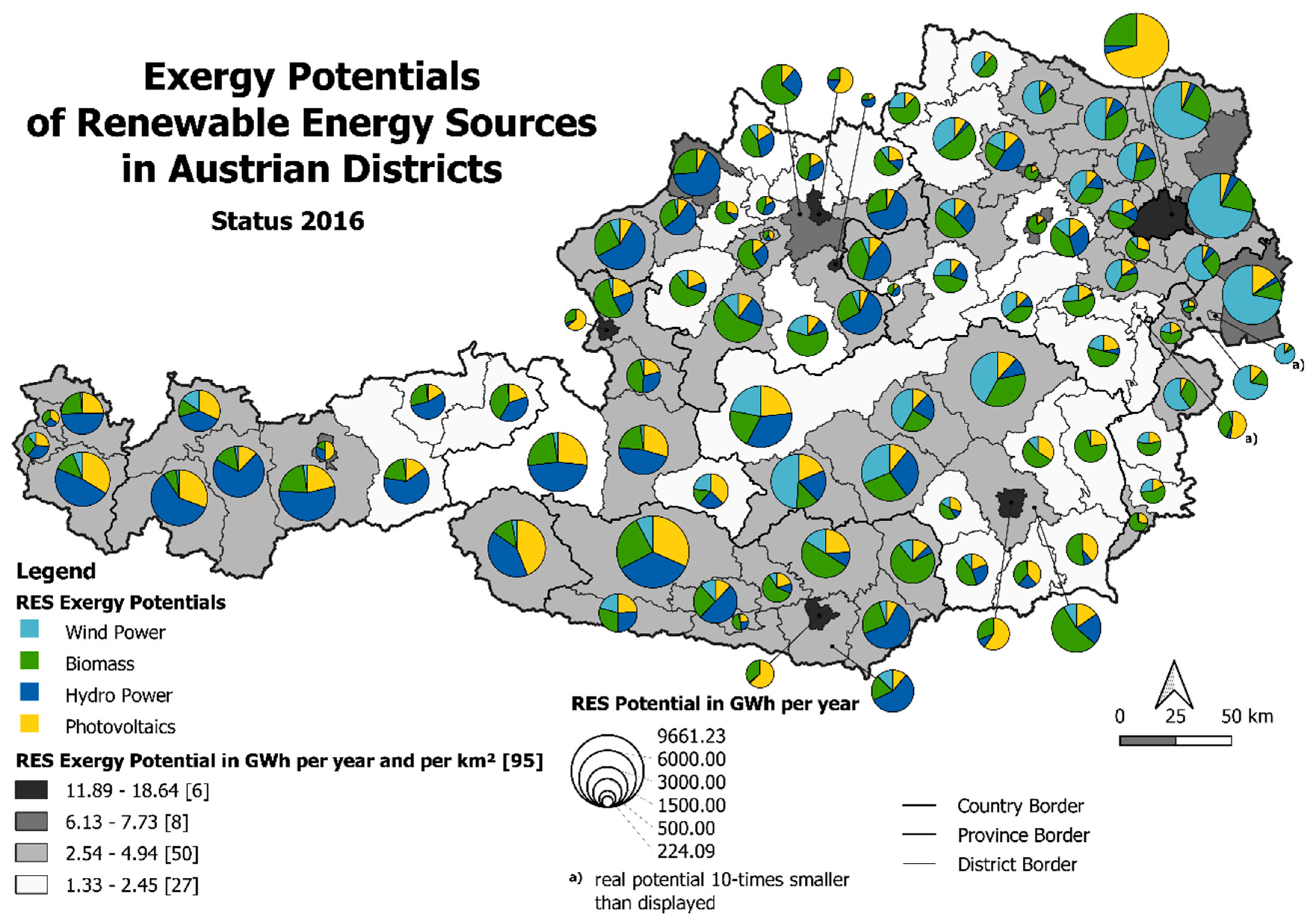
4.4. Spatially Resolved Technical Potential of Renewable Energy Sources

In this section, we discuss the determination of a spatially resolved renewable potential of Austria. This is the last of the three exergy amounts. This analysis is based on previous research [4,129,130] and has been further developed with the focus on an increase in spatial resolution. In this study, the renewable potential for each municipality in Austria is determined.

This paper covers the following renewable energy sources: solar thermal systems, photovoltaic, different forms of biomass, wind power, hydro power, geothermal energy and ambient heat. However, due to the exergetic focus of this paper, some energy sources were excluded:

• Ambient heat, which might be used in other studies, cannot be considered since per definition it has no exergy content.
• An exergetic comparison between solar thermal systems and photovoltaics showed that photovoltaics has an exergy output that is higher than the one of solar thermal systems, even if the energy output of solar thermal is 4 to 5 times higher: The total system efficiency of modern photovoltaics is about 16% to 17% [131], which is equal to the exergetic efficiency since electricity has an exergy factor of 1. In contrast, a solar thermal system with a high efficiency of 80%, hot water temperature of 75 °C and a surrounding temperature of 10 °C has an average exergetic efficiency of 15%. Therefore, in this study, only photovoltaics were considered. In addition to the higher efficiency, electricity has additional benefits as it is easier to transport and can be used for various applications.
• The geothermal energy potential was not considered in this paper since most of the geothermal potential has a low exergy content due to the low temperature difference to ambient heat, where a heat pump is necessary to make the heat accessible (comparable to ambient heat as a potential). Geothermal potentials with higher temperatures were also not considered in this study due to the low potential. In 2050, the extended potential of geothermal energy in Austria is estimated as 3062 GWh/a [132], which is equivalent to an exergy potential of less than 1 TWh/a and therefore, will not change the overall result (assumed temperature of the hot water is 150 °C since in Austria the highest water temperature of a geothermal application is in Bad Blumau with 143 °C [132]).

Since some renewable energy carriers are difficult to utilize (e.g., sewage sludge has a very low dry matter content), they are not balanced until they are converted into a generally usable energy carrier (e.g., conversion of sewage sludge to biogas). This corresponds to the IEA guidelines. Therefore, all considered renewable energy carriers (e.g., electricity, biogas, wood) have an exergy content of 100%.

Since there are different types of potentials, it is important to clarify that all potentials shown in this study are technical potentials. The definition of technical potential is discussed in Section 3.3. Technical potentials in general, and for the purpose of this study, do not differentiate between currently utilized or currently not utilized potentials.

4.4.1. Photovoltaic

The most important influence for the determination of a spatially resolved photovoltaic potential are the usable areas. Usable areas are orientated southwards with as little shading as possible. For example, these areas may be grassland, arable land, building facades or roofs. The energy output of a photovoltaic cell scales linearly with the area. In this work, only rooftops and fallow land, including currently unused agricultural areas, were considered.

The spatially resolved PV potential of rooftops is based on the publicly available data provided by OSM. OSM includes the positions as well as the floor area of over 85% of all buildings in Austria, which means that this data set can be considered as nearly complete [133].

The combination of the spatially resolved building data from OSM and the solar rooftop cadaster of the Austrian province Styria [134] allows the determination of the spatially resolved PV rooftop potential. This cadaster is provided by the Styrian government and describes the PV potential of each rooftop in Styria. It considers orientation and tilt of the rooftop but also shading [135]. An analysis of the combination of the OSM data and the solar rooftop cadaster of Styria showed that there is a linear relation between the sum of all floor areas and the sum of all PV potentials per municipality (coefficient of determination of this linear regression is R² = 0.86). Graz was not included in this linear relation since it is one order of magnitude bigger in terms of inhabitants than all the other municipalities of Styria [136].

To compensate for the lack of data of PV rooftop potential on a national level, the following assumptions were made in order to extrapolate the PV potential for each municipality in Austria based on the total sum of floor areas:

• For municipalities with up to 100,000 inhabitants, the factor from the linear correlation is used.
• For municipalities with 100,000 up to 300,000 inhabitants, the specific value of Graz is used.
• For Vienna, the officially published PV potential is used [137].

In this paper, the following types of land use were considered unused land (based on [138,139,140]): meadows yielding only one crop of hay per year, common pastures, bedding meadows, grasslands where the formation of steppe, woodland and scrub is prevented and no agricultural use is made, and land no longer farmed/unused greenland. Based on this definition, the spatially resolved PV potential of unused land can be determined by the area of unused land per municipality and a mean value of 8.9 acres/MW_ac (approx. 36,017 m²/MW_ac) [141]. In this calculation, it was assumed that only 50% of the total unused land can be used for PV due to shading [4]. In all PV relevant calculations, and that the annual PV full load hours were considered with 1000 [142,143].

4.4.2. Biomass

Biomass has various well-known paths of use. However, there are also applications in which the direct use of biomass is not possible (e.g., as fuel for a car). In these cases, the biomass has to be converted to a secondary energy carrier, such as biogas or biofuel to make usage possible. There are three different ways of converting biomass: thermo-chemical conversion (e.g., gasification of biomass), physical-chemical conversion (e.g., production of vegetable oil) and biochemical conversion (e.g., fermentation of biomass to biogas) [144].

In this work, different types of biomass potentials were considered: wood, wood products and wood waste, black liquor, biogas from various biogenic waste as well as fuels from field crops. Wood, wood products and black liquor were taken into account directly, without any conversion, since they can be utilized directly in furnaces. The exergy potential was calculated by multiplying the amount in tons per year with its higher heating value.

The spatial segmentation in this section was done as before: the total potential (for some biomasses available per province, for some only on a national level) of each biomass was allocated to the individual municipalities by a factor. This factor might be the number of inhabitants per municipality, the total area of the municipality, or the number of people working in a specific sector per municipality. As an example, to calculate the wood waste potential per municipality, the total potential of wood waste was divided by the total number of people working in the wood processing industry nation-wide and multiplied by the number of people working in this industry sector in the specific municipality.

The amount of wood, wood products, wood waste, and black liquor is available per province was spatially resolved by using the forest area, the number of people working in the wood processing industry as well as the number of people working in the pulp and paper industry per municipality (

Table 6. Considered wood, wood products, wood waste, and black liquor.

Type	Amount	Higher Heating Value	Spatial Segmentation
Forest (currently unused) 1	3.48 million m3/a 2 [145]	2696 kWh/m3 3	forest area
Firewood and wooden pellets	18,482 GWh/a [2]	−	forest area
Wood waste	23,767 GWh/a [2]	−	numbers of people working in the wood processing industry
Black liquor	9073 GWh/a [2]	−	number of people working in the pulp and paper industry

¹ Difference between forest growth and forest use, ² calculated with 20% crop losses [144,146], ³ calculated with the actual share of the different tree species in Austria [145] and the higher heating value (water content 0%) as well as the specific density for each tree species [144].

).

The potential of each type of biogenic waste was calculated by the amount of waste multiplied by the specific gas yield. Since the total amount of farm manure and sewage sludge in tons per year is unknown, the methane potential was calculated by the gas yield per animal or per population equivalent and the number of animals or the number of population equivalent, respectively. All other waste types are published in tons per year. In some cases, these amounts of waste are available for each province, in the other cases, they are only available on a national level. In order to ensure the best possible accuracy, the amount of waste per province was used wherever possible. The factor for the spatial segmentation is specific for each type of waste (

Table 7. Considered types of biogenic waste.

Type	Amount in t/a	Specific Gas Yield in Nm3 CH4/t Fresh Mass	Availability of Data	Spatial Segmentation
bio waste	530,700 [147]	103 [148]	Province	inhabitants
garden waste	482,800 [147]	64 [149]	Province	area
organic in residual waste	1,437,000 1 [147]	103 [148]	Province	inhabitants
public green waste	472,000 [147]	64 [149]	Austria	area
private composting	1,500,000 [147]	64 [149]	Austria	area
kitchen and food waste	113,400 [147]	205 2 [150]	Austria	inhabitants
cereal straw	2,526,326 3	153 [150]	Austria	cereal acreage
corn straw	2,208,831 4	82 [150]	Austria	corn acreage
rapeseed straw	162,959 5	97 [150]	Austria	rapeseed acreage
sugar beet leaf	6,713,538 6	47 [150]	Austria	sugar beet acreage

¹ Only 17.81% of this total amount of residual waste is organic [147], ² mean value of old bread, baking waste, cheese waste and food waste with a different share of fat, ³ calculated with a mean yield of 450 t cereal per km² [151], the total cereal acreage of 6122 km² [139] and a mean fruit-straw-ratio of 0.917 [144], ⁴ calculated with a mean yield of 1090 t corn per km² [151], the total corn acreage of 2026 km² [139] and a fruit-straw-ratio of 1 [144], ⁵ calculated with a mean yield of 280 t rapeseed per km² [151], the total rapeseed acreage of 540 km² [139] and a mean fruit-straw-ratio of 2.8 [144], ⁶ calculated with a mean yield of 7320 t sugar beet per km² [151], the total sugar beet acreage of 448 km² [139] and a mean fruit-straw-ratio of 1.7 [144].

and

Table 8. Considered sewage sludge and animal excrements as biogas potential. All values are only published for the whole of Austria.

Type	Amount	Specific Gas Yield	Spatial Segmentation
sewage sludge	14,209,529 PE60 1 [152]	14.5 Nm3 CH4/(PE60*d) 2	inhabitants
dairy cows	7,669,671 [153]	290 Nm3 CH4/(animal*a) 3 [154]	number dairy cows
fattening pigs	6,632,840 [153]	21 Nm3 CH4/(animal*a) 3 [154]	number fattening pigs
beef cattle	2,355,874 [153]	129 Nm3 CH4/(animal*a) 3 [154]	number beef cattle
chicken	86,775 [153]	1.4 Nm3 CH4/(animal*a) 3 [154,155]	number chickens

¹ The number of population equivalent 60 (PE₆₀) measures the pollution load in waste water. The average pollution load of one person in 24 h defines one population equivalent, ² calculated with an average value of 25 l biogas per PE₆₀ and day [156] as well as with the lower heating value of the biogas of 6.4 kWh/Nm³ [157], ³ calculated with the amount of excrement per animal and year as well as the specific gas yield.

).

In Austria, the biogas potential of waste from the food and beverage industry is 152 million Nm³ CH₄/a [130]. A spatial segmentation was achieved by the number of people working in the food and beverage industry per municipality.

Apart from different forms of wood, biogenic waste and farm manure, black liquor as well as sewage sludge, this study also takes the current Austrian production of biodiesel, bioethanol and biogas into account. Only the production of Austrian biomass for the Austrian market was considered. To avoid a competitive situation with food and feed production, the currently used areas for fuel and biogas production are not expanded (

Table 9. Current production of bio fuels and biogas using biomass from Austria.

Type	Amount	Spatial Segmentation
biodiesel from new oil	31,604 t/a 1 [158]	arable land
biodiesel from used cooking oil and other used fats	47,406 t/a 2 [158]	inhabitants
Bioethanol	185,669 t/a [158]	arable land
Biogas	967 GWh/a 3 [158]	arable land

¹ 40% of the total biodiesel production in Austria is based on new fruit or seed oil but only 26.8% of the total biomass input is biomass from Austria [158]. ² 60% of the total biodiesel production in Austria is based on used cooking oil and other used fats but only 26.8% of the total biomass input is biomass from Austria [158]. ³ In 2017, biogas plants in Austria produced a total of 565 GWh of electricity (mean efficiency of power units: 36.5% [154]) and 149 GWh of gas were fed into the public gas grid [158].

).

In addition to the techniques mentioned above, the fermentation residue of the biogas plants can also be used to produce some additional methane. For this purpose, the fermentation residue must first be dried and then gasified and methanized. The waste heat generated in the gasification and methanation can be used for drying fermentation residue. Overall, with this process, another 0.22 GWh biogas can be produced from the fermentation residue of 1 GWh biogas [130].

4.4.3. Wind Power

The maximum for attainable wind potential in Austria is published in the study “Windatlas und Windpotentialstudie Österreich” [71,159]. This potential considers all reasonable positions in Austria and can be compared to the technical potential of the other renewable energy sources mentioned in this section. Since this study [71,159] only publishes the maximum of attainable wind potential per province, a methodology for spatial separation had to be applied.

In general, the wind potential of a certain region can be estimated based on a uniform dot matrix. Each point of this dot matrix represents one possible wind farm. First, the whole region will be covered by this dot matrix. In the second step, some dots will be eliminated from the matrix, according to well-defined rules, e.g., distance to buildings. Finally, the potential per dot can be estimated in combination with the annual average wind speed [160].

This methodology was used for the segmentation of the maximum of attainable wind potential per province of Austria broken down into municipalities. To achieve this, the number of wind-speed-weighted dots per municipality was calculated. Thus, the maximum for attainable wind potential per municipality in Austria was calculated from the ratio of the number of wind-speed-weighted dots per municipality and the total number of wind-speed-weighted dots per province. In this work, a minimal distance to buildings of 1000 m and a maximum height above sea level of 2000 m was used (spatially resolved sea level of Austria: [161], spatially resolved annual mean wind speed: [160]). Dots in nature reserves and national parks were also excluded (spatially resolved nature reserves and national parks: [162]).

4.4.4. Hydro Power

The hydro power potential was taken from the study “Wasserkraftpotenzialstudie Österreich Aktualisierung 2018”. In this study, Pöyry Austria GmbH calculated the technical-economical potential, but also the technical hydro power potential of Austria. These potentials consider the flows of all rivers in Austria, their change in water level as well as in altitude. The technical potential assumes that 87% of the total flow potential can be harnessed. Since the spatially resolved technical potentials are only published in the form of a map, we analyzed this using the GIS application QGIS [163] and calibrated it based on Austria’s total potential. Furthermore, we used QGIS to quantify the technical hydro power potential per municipality. [72]

4.5. Generalization of the Approach

This study used Austria as an example for presenting the methodology of calculating the three spatially resolved exergy amounts: the current exergy consumption, the current useful exergy demand and the technical exergy potentials of RES.

The methodology shown is general and can also be used for other countries since the necessary energy statistics (e.g., final energy consumption per sector, transformation inputs and outputs, transport losses, consumption of energy sector use, etc.) are also published by Eurostat [1] or other comparable national statistics services or agencies. If necessary, the data of comparable countries can also be used (e.g., share of different final energy applications).

The methodology for exergetic analysis for determining current exergy consumption and the current useful exergy demand can be applied to other countries directly and, if necessary, the exergetic efficiencies for different applications (e.g., efficiency of stationary motor system), which are listed in Section 3.1.3, can be used.

Especially when determining the national technical potential of RES or the spatial separation of the national results, the methodology has to be adapted to the given data (e.g., already published potential studies, statistical data on spatial distribution of land use). However, since the methodology is mainly based on our own calculations, the basic ideas can be used generically (e.g., the methodology of determining the PV potential using OSM, using spatial segmentation factors, etc.).

5. Results

In this section, the results of applying the developed methodology to Austria (Section 4) are shown. For the presentation of the results, we use the structure introduced in Section 1. The results of the three exergy amounts will be discussed in Section 5.1. Furthermore, the Austria-wide and spatially resolved comparisons of the three exergy amounts are presented in Section 5.2 and Section 5.3, respectively.

5.1. Results per Exergy Amount

5.1.1. Current Exergy Consumption and Current Useful Exergy Demand

In this section, the results of the two exergy amounts, the current exergy consumption and the current useful exergy demand will be presented together, due to the comparable structure of the results. This leads to a clearer structure without repetitions. Please note, comparisons between these two exergy amounts are only made in Section 5.2.1 (Austria-wide) and in Section 5.3.1 (spatially resolved).

In accordance with the calculation shown in Section 4, the current exergy consumption in Austria amounts to 370 TWh/a, whereas the primary energy consumption amounts to 374 TWh/a. The calculated primary energy consumption (374 TWh/a) is slightly lower than the value reported by Statistics Austria for 2017 (381 TWh). The difference (less than 2%) is caused by the combination of bottom-up and top-down approaches and by various data sources from varying years.

The current exergy consumption is nearly equal to the calculated total primary energy consumption of Austria, since over 98% of the primary energy consumption of Austria is covered by high exergetic energy carriers (e.g., imported natural gas, electricity from photovoltaics or extracted crude oil). The remaining primary energy consumption is covered by energy carriers with a low exergy value (solar thermal energy) or no exergy content at all (ambient heat). The final energy demand of other low exergetic energy carriers (geothermal energy and reaction heat) as well as the transformation input of solar thermal and geothermal energy are neglectable, since they are in total being less than 0.1% of the primary energy consumption in 2017. According to the calculation in Section 4, the current useful exergy demand of all sectors amounts to 125 TWh/a, which is significantly lower than current exergy consumption.

For the spatially resolved visualization of the current exergy consumption and the current useful exergy usage, district resolved maps are used (Figure 7 and Figure 8). In these maps, one can see the absolute exergy consumption or demand per district, represented by the size of the pie charts. In addition, the pie charts also illustrate how much exergy is needed in which sector. Since the absolute value per district is dependent on the respective district area, the relative consumption or the relative demand per district is represented by the gray scale. To calculate the relative consumption or relative demand per district, the current exergy consumption or the current useful exergy demand, respectively, is divided by the area. Please take note of the different scales of all maps. A spatial overview of all provinces and districts in Austria can be found in Appendix B (Figure A1).

In Austria, the maximal relative current exergy consumption and current useful exergy demand are located in urban areas. These are cities such as Vienna, Graz, Linz, Innsbruck or Klagenfurt, including their surroundings. In addition, industrial regions, e.g., Upper Austria, Lower Austria, and Styria, also have a high relative exergy consumption and demand. One can see that the absolute exergy usage and demand are highest in Vienna and Linz. In terms of absolute consumption and demand, these two cities are comparable, but the share of the sectors is very different.

The high relative exergy consumption in urban areas can be explained by the population density. For example, in Vienna, 35% of the current exergy consumption is caused by transport, 31% by the residential sector, 24% by commercial and public services and only 9% is caused by industry (agriculture in Vienna is neglectable). The fact that the city of Linz has an absolute exergy consumption comparable to Vienna, but has a very different share of the sectors, is due to a smaller population and a strong industrial sector. Linz only has around 11% of the population of Vienna [114] but has a strong energy intensive industry, such as an iron and steel mill with three blast furnaces. Therefore, in Linz, 84% of the current exergy consumption and 93% of the current useful exergy demand are caused by industry. In general, areas with a high share of energy intensive industry (industries which are obliged to participate in emission trading [164,165]) have a higher relative exergy consumption and a higher relative exergy demand.

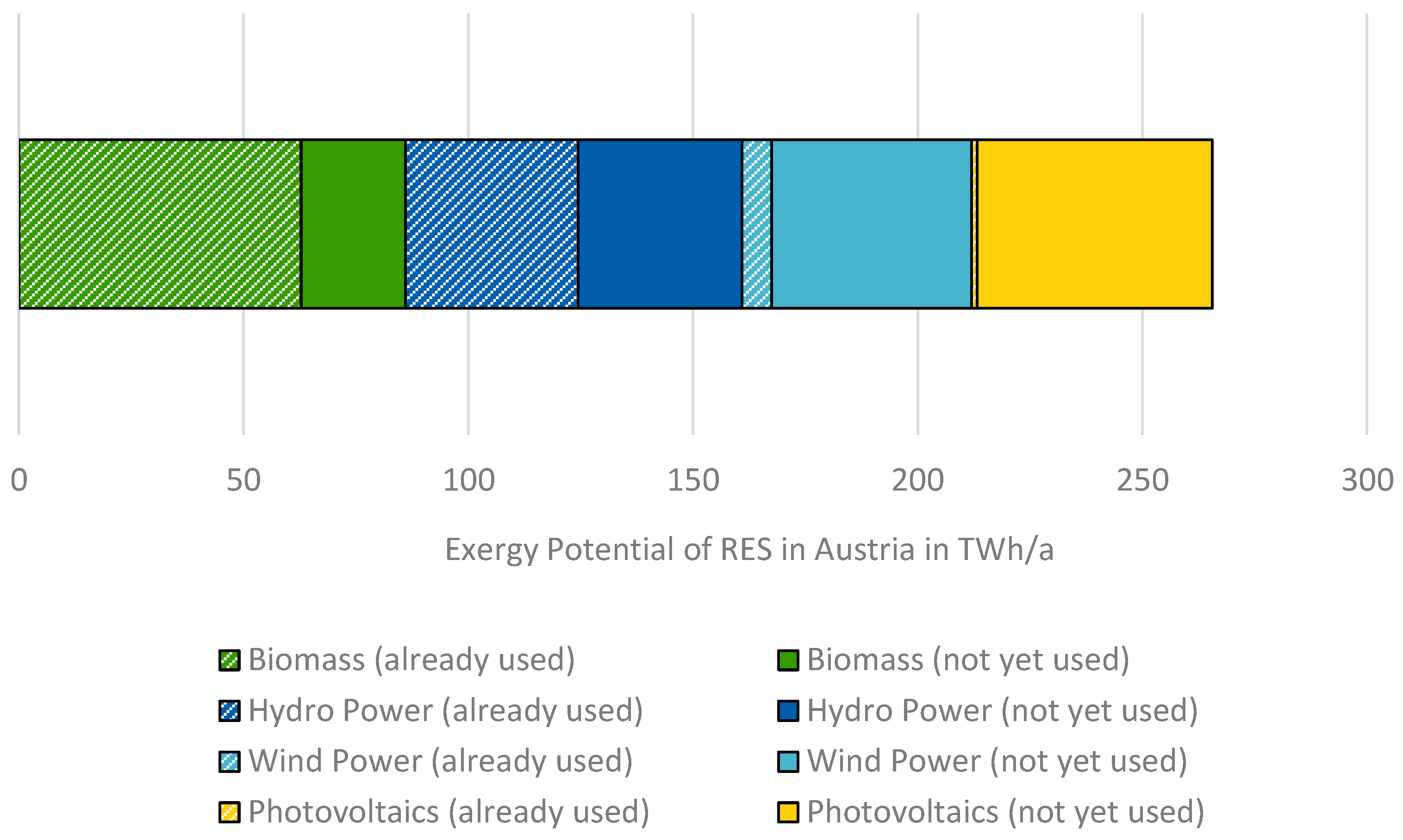
5.1.2. Technical Exergy Potentials of RES

In this section, the exergy potential of RES in Austria will be discussed. The exergy potential consists of hydro power (75 TWh/a), photovoltaics (54 TWh/a), woody biomass (52 TWh/a), wind power (51 TWh/a), biogas and biofuels (25 TWh/a), as well as black liquor (9 TWh/a). In total, the exergy potential amounts to 266 TWh per year. The spatially resolved potential for each district of Austria is shown in Figure 9. For simplicity, the potential is shown for each district, although it is calculated for each municipality of Austria individually. Since, per definition, all of the considered potentials of RES have an exergy content of 100% (Section 4.4), this exergy potential is equal to the primary energy potential of RES.

Figure 9 contains a variety of information. The total technical exergy potential of RES per district is represented by the size of the pie chart. The slices of the pie chart show the share of different renewable energy sources per district. Additionally, the relative potential per district, which is the total potential divided by the area, is visualized by the different shades of gray. Please take note of the different scales of all maps. A spatial overview of all provinces and districts in Austria can be found in Appendix B (Figure A1).

In Figure 9, one can see that there are huge regional differences in the share of the different renewable energy sources. Urban regions tend to have a higher proportion of photovoltaics and biomass (e.g., cities such as Vienna, Graz, Linz, Salzburg) while wind power is most dominant in the north-east of Austria. There is a large share of hydro power in the west and south-west of Austria, but also along the rivers Danube and Inn. Apart from the share of the different energy sources, the relative exergy potential in Austria is relatively equally distributed (mean value: 4 GWh/(a⋅km²), standard deviation: 3 GWh/(a⋅km²)). Only seven districts have a higher potential than the average plus standard deviation (>7 GWh/(a⋅km²)) and there are no districts that have a lower potential than mean value minus standard deviation (<1 GWh/(a⋅km²)).

The share of PV and biomass in urban regions can be explained by the high number of rooftops, which can be used for photovoltaics, and the biomass potential in these areas is mainly based on the high population density: a high number of inhabitants cause a lot of organic waste (e.g., bio waste or food and kitchen waste as well as sewage-sludge) which can be utilized in biogas plants. However, rural regions also have photovoltaic (unused land) and biomass (agricultural, residuals, forests, wood waste and black liquor) potential. Therefore, every district of Austria offers photovoltaic and biomass potential, but the share varies strongly.

In Austria, the highest average wind speeds are found in the north-east, mainly due to the topography [160], resulting in comparatively high wind potentials in this area. The mountain area in the west and south-west enable hydro power potentials due to the height difference. In general, it can be stated that there are large hydro power potentials where large annual precipitation takes place, as well as where large and water-rich rivers (e.g., Danube, Inn, Enns) are located.

5.2. Austria-Wide Comparisons of the Exergy Amounts

In this section, the three exergy amounts (current exergy consumption, current useful exergy demand as well as the technical exergy potential of RES) are compared Austria-wide. A visual comparison of the three exergy amounts is shown in Figure 10. It shows that the current exergy consumption is higher than the technical potentials of RES. Thus, based on its current exergy consumption, Austria cannot supply itself with renewable energy. However, self-sufficiency can be achieved by a significant reduction in the current exergy consumption towards the current useful exergy demand. This could be achieved by increasing the overall exergy efficiency. In Section 5.2.1, Section 5.2.2 and Section 5.2.3, more detailed comparisons between the different exergy amounts are presented.

5.2.1. Current Exergy Consumption and Current Useful Exergy Demand

The comparison of the current exergy consumption with the current useful exergy demand shows the total exergy efficiency of the overall energy system in Austria: 370 TWh/a of exergy is consumed in order to cover 125 TWh/a of actually useful exergy demand (Figure 10). The difference between these two exergy amounts is the exergetic loss of the whole system. This total loss includes conversion losses, transport losses as well as losses in the final energy application. Austria has a total exergetic loss of 245 TWh/a and, therefore, an overall exergetic efficiency of 34%.

Among all sectors, the industrial sector has the highest current exergy consumption, followed by the transport and the residential sectors. The exergetic efficiency is 49% (industrial sector), 27% (transport sector), 26% (commercial and public services), 20% (residential sector) and 14% (agriculture), respectively (

Table 10. Austria-wide comparison of the current exergy consumption and the current useful exergy demand per sector, including the exergetic efficiency. The efficiency is the highest in the industrial sector, since it needs a lot of heat at high temperature levels.

Sector	Current Exergy Consumption in TWh/a	Current Useful Exergy Demand in TWh/a	Exergy Efficiency in %
Industry	140	68	49
Transport	112	31	27
Residential sector	75	15	20
Commercial and public services	36	9	26
Agriculture	7	1	14

).

In addition, an even more detailed, subsector-resolved comparison is presented in Figure 11 and Figure 12. The ratio between current exergy consumption and current useful exergy demand can be used to determine the efficiency per subsector. The exergetic loss per subsector is the difference between these two parameters.

The exergetic losses per subsector are shown in Figure 11 and Figure 12. The greatest losses occur in road-based transport (71 TWh/a), followed by the residential sector (60 TWh/a), commercial and public services (27 TWh/a), pulp, paper and print (14 TWh/a), and iron and steel (12 TWh/a).

Since the energy supply in all sectors is almost exclusively based on highly exergetic energy carriers, the large differences in efficiency between the different sectors (industrial, residential sector, commercial and public services, agriculture) can be explained by the different temperature levels of the heat demand. The industrial sector has a high share of the process heat demand on high temperature levels, while the residential sector, commercial and public services, as well as agriculture, need mainly heat on a low temperature level (e.g., for space heating and hot water (Table A2)). Thus, the exergetic efficiency is much lower.

The exergetic efficiency of the transport sector is limited due to the predominance of internal combustion engines and their characteristics. Figure 11 and Figure 12 show that exergy is currently used incorrectly, especially in the field of transport and low-temperature applications such as space heating.

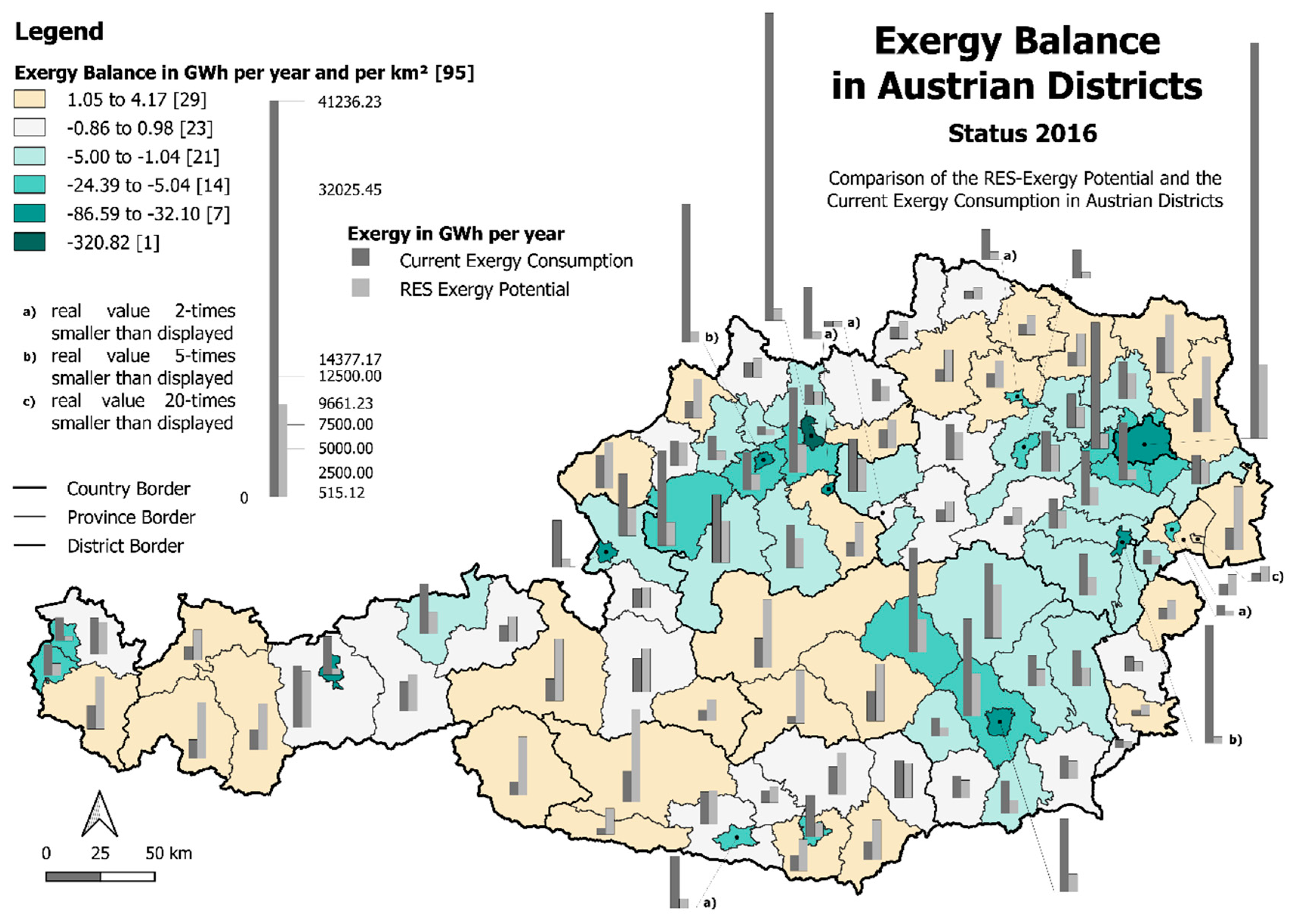
5.2.2. Current Exergy Consumption and Technical Exergy Potentials of RES

The Austria-wide comparison shows that the current exergy consumption is higher than the technical exergy potential of RES (Figure 10). In order to enable renewable self-sufficiency, the exergy consumption would have to be reduced by at least 105 TWh/a, which is 28% of the current exergy consumption. Alternatively, for a completely renewable supply for Austria, renewable exergy imports (e.g., electricity or hydrogen) are necessary.

However, the reduction in the current exergy consumption by 105 TWh/a and a complete expansion of all technical potentials of RES would almost certainly not be enough, since large shares of volatile energy sources are considered in the technical exergy potential (e.g., photovoltaics or wind power). These volatile energy sources require a corresponding infrastructure, which must ensure uninterrupted energy and exergy supply, regardless of the weather or the season. Conversion, storage or transport losses caused by the required infrastructure will have higher losses in the future due to the change in operating mode. A consideration of the infrastructure necessary in the future is explicitly not part of this paper. It will be addressed in further research.

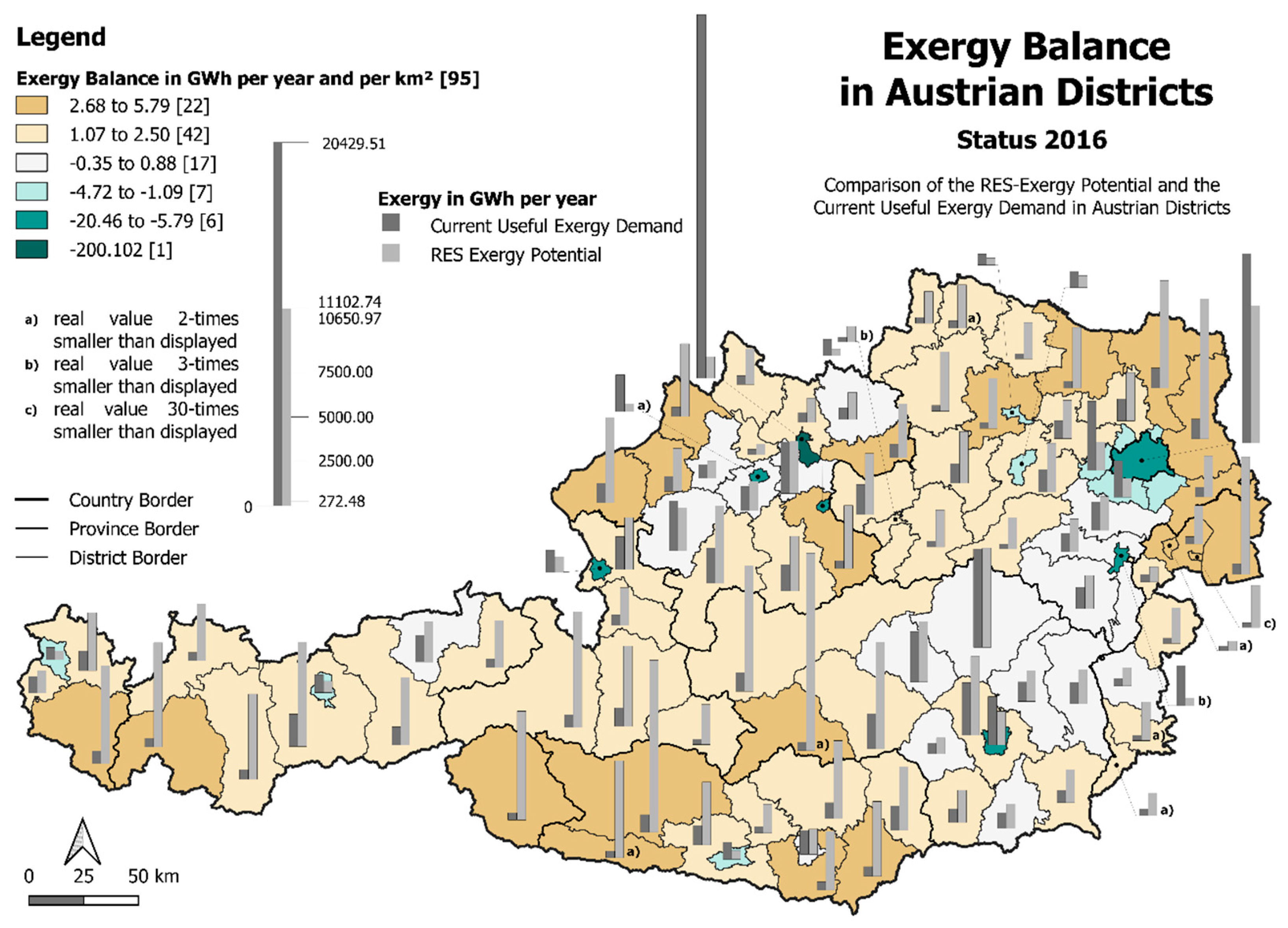
5.2.3. Current Useful Exergy Demand and Technical Exergy Potentials of RES

The current useful exergy demand is much smaller than the exergy potentials of RES in Austria (Figure 10). Thus, if all energy services needed were provided in a way that is exergy optimal, Austria could easily supply itself with renewable exergy. In this exergy optimal case, only about 47% of the total exergy potentials have to be utilized. However, it does not take any exergy losses of the energy supply (mentioned in the previous section) and of the used technology, which provides useful energy, into account. If these losses are also considered, more than 47% of the technical exergy potentials have to be utilized. The difference between the current useful exergy demand and the technical exergy potential of the renewables (141 TWh/a) can be used to cover the losses mentioned. However, the determination of the best technology for final energy applications is explicitly not part of this paper and will be addressed in further research.

5.3. Spatially Resolved Comparison of the Exergy Amounts

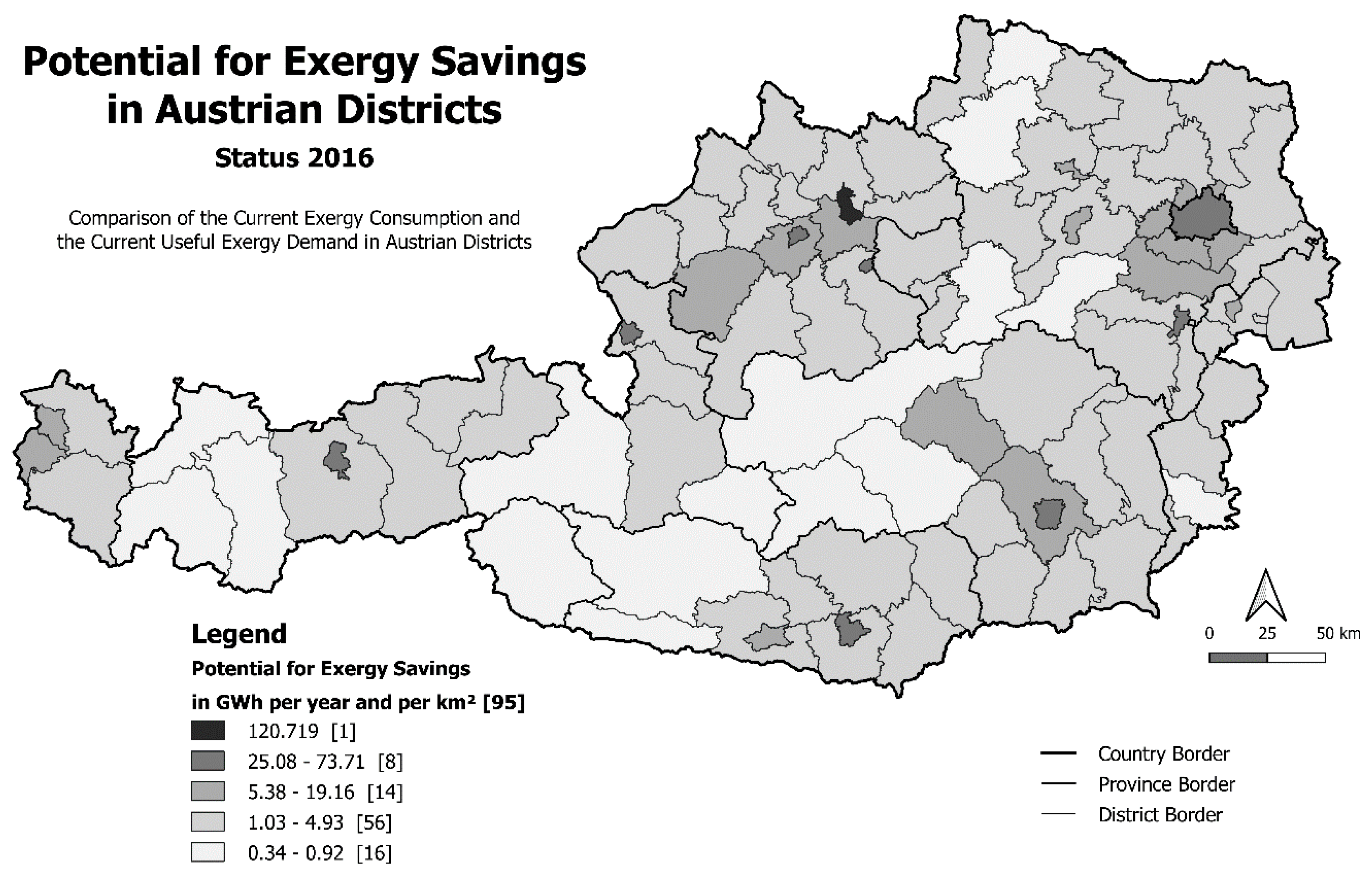
5.3.1. Current Exergy Consumption and Current Useful Exergy Demand

The spatially resolved comparison between the current exergy consumption and the current useful exergy demand shows the relative potential for exergy savings per district (Figure 13). It is calculated for each district by subtracting current useful exergy consumption from current exergy consumption, divided by the area of the district. The gray scale ranges from light gray (minimum potential for savings) to dark gray (maximum potential for savings). Please take note of the different scales of all maps. A spatial overview of all provinces and districts in Austria can be found in Appendix B (Figure A1).

Figure 13 shows that the greatest relative potential for exergy savings can be found in the city of Linz. However, all other urban areas, such as the major cities and their surrounding areas (e.g., Vienna, Graz, Innsbruck or Klagenfurt), as well as some industrial areas, also have large relative potential for exergy savings.

The distribution of the spatially resolved potential for exergy savings can be explained by a direct comparison with the spatially resolved current exergy consumption (Figure 7). Therefore, areas with a currently high exergy consumption also show the greatest potential for exergy savings. The statistical analysis between the current exergy consumption and the current useful exergy demand shows that in Austria, the exergy efficiency per district is rather homogeneous (mean value 31%, standard deviation 7%).

In a district-resolved comparison of the current exergy consumption (Figure 6) with the current useful exergy demand (Figure 7), the share of industry is generally greater for current useful exergy demand than for current exergy consumption. This is mainly caused by the high processing temperatures of the industrial heat demand in contrast to the low temperatures for space heating and hot water.

5.3.2. Current Exergy Consumption and Technical Exergy Potentials of RES

The spatially resolved comparison of the two exergy amounts—current exergy consumption and technical exergy potentials of RES—is shown in Figure 14. The map shows the difference between the current exergy consumption and the technical exergy potentials of RES.

In this map, there is a bar chart for each district. These bar charts show the absolute consumption (dark gray) and the absolute potential (medium gray) per district. The balance, which is the difference between these two bars, indicates if a district can exergetically supply itself or not. The relative balance, which is the balance divided by the area of the district, is visualized in the background by the shades of color from ocher to blue-green. In ocher colored districts, the potential is higher than the usage or demand, while blue-green colored districts indicate where the potential is smaller than the consumption. Light gray colored districts are almost balanced. Please take note of the different scales of all maps. A spatial overview of all provinces and districts in Austria can be found in Appendix B (Figure A1).

This spatial comparison shows that nearly all districts, with high relative exergy consumption (Figure 7) also have a negative exergy balance (Figure 14). Especially urban areas have a negative relative exergy balance. The area with the worst relative exergy balance is Linz (approx. −321 GWh/(a⋅km²)), followed by Steyr (approx. −87 GWh/(a⋅km²)) and Vienna (approx. −81 GWh/(a⋅km²)). On the other hand, 52 of 95 districts in Austria have a positive relative balance or are approximately balanced.

The reason why this map is comparable to current exergy consumption is that the exergy potential is rather evenly distributed in Austria (standard deviation: 3 GWh/(a⋅km²)), while current exergy consumption has a wide variation (standard deviation: 38 GWh/(a⋅km²)). Therefore, the difference in the exergy potential cannot significantly change the distribution of the current exergy consumption.

Based on these findings, large energy and exergy flows from the whole of Austria to urban and industrial regions will be necessary in the future. What the infrastructure necessary in the future should look like cannot yet be estimated based on this map, since this paper does not consider the time perspective.

5.3.3. Current Useful Exergy Demand and Technical Exergy Potentials of RES

The last spatially resolved comparison of two exergy amounts is shown in Figure 15. This comparison includes the current useful exergy demand as well as the technical exergy potential of RES. The concept of this map is equivalent to the description in Section 5.3.2. Accordingly, we now refer to the explanation of the map in the previous section.

The spatially resolved relative balance between the current useful exergy demand and the technical exergy potentials of RES is very different, from the balance in the previous Section (Figure 14). In this comparison, almost all districts of Austria have a greater potential than demand, or are almost balanced. Only a few urban areas still have a negative balance (e.g., Linz: −200 GWh/(a⋅km²), Steyr: −20 GWh/(a⋅km²), Wels: −18 GWh/(a⋅km²)). Eighty-one of 95 districts of Austria have a positive relative exergy balance or are nearly balanced (e.g., the industrial regions in Styria and Upper Austria).

This significant difference compared to Figure 15, where only 52 of 95 districts have a positive exergy balance, can be explained by the fact that current useful exergy demand is only about 34% of current exergy consumption.

Figure 15 shows that the excess of the oversupplied districts must be used to supply districts with a negative balance. Therefore, in the future, one challenge will be the exergy transport from the generation site to the consumption site, even if the exergy consumption can be reduced to the current useful exergy demand. Such a significant reduction can only be achieved by changing the used processes and/or the energy service demands.

6. Discussion

In the last few years, different studies have shown that Austria cannot supply itself with renewable energy, even if all renewable potentials are used [4,129,166]. The novelty of this work is that the comparison of the potential and the consumption is made on an exergy level. A comparison of different energy forms (e.g., electricity or heat) and energy carriers (e.g., natural gas, coal, hot water) is more reasonable on an exergy level since exergy considers the quality of energy. Exergy can also be used to determine the actual need of any energy service. Therefore, exergy allows for a much better comparison than energy.

Primary energy consumption, in contrast to final energy consumption, also takes into account the losses of industrial conversion (3% of the primary energy consumption), industrial energy sector use (7% of the primary energy consumption), transport losses (2% of the primary energy consumption), as well as the energy supply system itself (6% of the primary energy consumption). Whether or not this 18% of the primary energy consumption must be considered depends on the specific application. As this paper aims to give a comprehensive overview of the situation in Austria, all these losses must be considered. Therefore, we use the primary energy consumption of Austria as a basis for the determination of current exergy consumption.

In principle, the energy that flows into the system and the energy that flows out of the system is first balanced and then exergetically evaluated. On the one hand, the primary energy consumption is balanced, which is the energy that flows into the national energy system. On the other hand, the useful energy, which is actually needed by all energy services in Austria, is also balanced (Figure 5). The characteristic of services is that they provide useful energy by using final energy. Since the service demand is technology independent, it is reasonable to describe it by the actually required work, which is exergy. According to thermodynamics, the actual exergy demand of a service is equal to the theoretical minimum of the final energy demand of any final energy application. This theoretical minimum can only be reached if the final energy application has no losses and the energy is supplied on the application specific optimal exergy level.

In addition, the Austrian technical potentials of RES are also taken into account in this paper. Subsequently, all three of these so-called exergy amounts were compared, firstly on an Austria-wide basis and then spatially resolved (Figure 1).

6.1. Austria-Wide Results

In Austria, the present energy system, which also includes the final energy utilization, has an exergetic efficiency of 34%. In 2005, Gutschi et al. [3] calculated an exergetic efficiency of about 21% for Austria. The increase can be explained on the one hand by different assumptions (e.g., reference temperature, required temperature levels) and on the other hand by different reference years. For comparison, according to [36], the exergy efficiency of other countries is between 15% and 39%. Due to this low efficiency, Austria cannot cover its exergy consumption with its own exergy potentials of RES. Therefore, in the present energy system, exergetic imports (e.g., hydrogen or electricity) are necessary to realize renewable and CO₂-neutral supply of primary energy. To avoid such primary energy imports, the efficiency of the energy system must be significantly increased. Thus, the final energy utilization and its current technologies must be changed. The following sectors have the lowest exergy efficiency of their final energy applications: agriculture (14%), residential sector (20%) and transport (27%).

In this work, two aspects are not considered. On the one hand, the exergy of waste heat could also be added to the exergy potentials. Such cascaded energy and exergy utilizations increase the efficiency of the overall energy system. For example, the high-temperature waste heat could be used to supply a medium temperature process. Then, the waste heat of the medium temperature process might be used to provide heat at a low temperature level such as for space heating.

On the other hand, this paper also does not include a concept regarding how a future energy supply infrastructure and how the future final energy utilization technologies might look like in order to ensure the highest possible exergy efficiency. Such a concept is necessary to determine how much the current useful exergy demand must be increased, in order to calculate the lowest possible exergy demand. However, further research is required to achieve this.

6.2. Spatially Resolved Results

A spatially resolved holistic view of the Austrian energy system has only been published in the recent work of Abart-Heriszt et al. [5]. The spatially resolved energy consumption in their work was based on very similar approaches and data sources as this work. Probably the most important distinction is that the work of Abart-Heriszt et al. was based on the final energy consumption, while this work is based on the primary energy consumption.

Abart-Heriszt et al. [5] analyzed the different types of land use for the municipalities’ energy consumptions and greenhouse gas emissions. Furthermore, they calculated spatially resolved greenhouse gas emissions. In addition to that, in this work, we calculated and compared spatially resolved current exergy consumption and the current useful exergy demand, as well as the technical exergy potential of RES.

The spatially resolved analysis showed that the renewable potential is rather evenly distributed across Austria (standard deviation: 3 GWh/(a⋅km²)), although the share of the different renewable potentials varies significantly. In contrast to that, the exergy consumption is mainly located in industrial regions and urban areas (standard deviation: 38 GWh/(a⋅km²)). Rural regions show significantly lower exergy consumption. Therefore, in the future, exergy flows from rural regions to industrial and urban areas will be necessary.

6.3. Exergy Potentials of RES

In this study, the spatially resolved technical exergy potential of RES in Austria was calculated. Compared to other Austria-related potential studies, this is the only one based on exergy. Therefore, only selected energy carriers are considered: photovoltaics, wind power, hydro power, and biomass. Solar thermal energy is not taken into account since an exergetic analysis showed that the exergy potential of photovoltaics and the exergy potential of solar thermal energy per area is comparable. The Austrian geothermal potential and ambient heat are also excluded, since the geothermal potential is very limited, and the exergy content of ambient heat is zero per definition. According to IEA guidelines, energy carriers which are difficult to utilize (e.g., sewage sludge) are only taken into account after the conversion to secondary energy carriers (e.g., biogas or biofuels).

A comparison of the already used (reference year 2017, data source: [2]) and currently unused exergy potential of RES in Austria is shown in Figure 16. In this figure, only those energy carriers are taken into account that were also used to calculate the exergy potential in this study. The excluded energy carriers (geothermal, ambient heat, solar thermal and reaction heat) have an overall energy generation of 5 TWh/a [49], but an exergy content of only 0.5 TWh/a (assumed temperatures: solar thermal energy 75 °C, geothermal energy 150 °C, reaction heat 100 °C, ambient heat and surrounding temperature 10 °C). This figure shows that Austria already uses a huge amount of the total available biomass and hydro power potential, but only a very small share of the photovoltaics and wind power potential. Therefore, the utilization of wind and photovoltaics could be increased by about eight and 42 times, respectively.

This potential study is difficult compared to other Austria related studies, as it is the only one which is based on exergy, instead of energy. Different types of potential are calculated, assumptions may be different (e.g., competition for area) and different energy carriers are taken into account. Therefore, one cannot directly compare the results of different studies. However, if one neglects energy carriers with no exergy content (e.g., ambient heat) and estimate the exergy content of energy carriers with a low exergy content (e.g., solar thermal systems), it becomes clear that the overall potential of all studies, including this one, are in the same order of magnitude. For comparison, the energy potential of technical potential studies of RES in Austria varies between 266 and 606 TWh/a (Section 3.3.2).

6.4. Uncertainty Analysis

In this section, the uncertainty of the results is discussed. This work is based on different data sources such as statistics, scientific papers or reports. The uncertainty of these data sources is due to their methodology. Where appropriate data are missing, assumptions had to be made. Assumptions that affect energy or exergy only to a small extent do have minor effects on the overall result. The determination of the Austria-wide current exergy consumption and current useful exergy demand is based on only a few assumptions:

• Since the actual share of different light sources in the different sectors in Austria is not published, the share of lighting technologies in the German commercial and public services is used for all sectors in Austria. Lighting causes only about 2% of the primary energy consumption in Austria.
• The sources of the actually used heat temperature statistic (Table A2) do not include the temperature levels of the process heat demand (not space heating) in the sectors agriculture, and commercial and public services. In Austria, the process heat demand of these two sectors is only approx. 2% of the primary energy consumption.
• Where an efficiency or a temperature range is published, we used the mean value of this range. For an Austria-wide analysis, due to the high number of energy and exergy consumers (industrial sides, households, etc.), this mean value should be fairly accurate.
• Self-consumption of power plants, as well as the energy needed for pumping (e.g., for natural gas or district heating), is allocated to the total fossil (except road-based transport, railways, inland navigation and aviation), electrical and district heating energy consumption, since no detailed data are published. The self-consumption of power plants and consumption for pumping is only 1% of the primary energy consumption.
• The quality factor of chemical energy carriers is assumed as 1 (Section 2.1), since the actual values are difficult to calculate (consideration of all physical and chemical aspects of the surroundings) and no significant deviations occur.
• Due to the usage of a combination of top-down and bottom-up approaches and the usage of various data sources from varying years, there is a difference of about 2% in primary energy consumption between the calculated value and the value published by Statistics Austria (2017).
• Some low exergetic energy carriers (final energy demand of geothermal energy and reaction heat as well as transformation input of solar thermal and geothermal energy) are neglected as they account for less than 0.1% of the total primary energy consumption in 2017.

Based on this uncertainty analysis, current exergy consumption and the current useful exergy demand are reliable (or as reliable as the sources used), since the assumptions cannot significantly change the results.

In contrast, the assumptions that explain the biggest uncertainties are made for determining the spatially resolved results, since a lot of different information is required. For this, not all needed data are published. Due to the lack of available information, there were assumptions necessary to enable spatially resolved results. The main assumptions are:

• Linear correlation of the industrial primary energy consumption and the employees per industrial subsector
• Linear correlation of the primary energy consumption of agriculture and the employees in this sector
• Linear correlation of the primary energy consumption of commercial and public services and the employees in this sector
• Linear correlation of the residential primary energy consumption and the population
• Spatial segmentation of the renewable biomass potential per segmentation factor
• Spatial segmentation of the transport based on the infrastructure.

Whenever possible, the quality of the data was improved by combining different approaches or data sources. For example, for industry, the quality of the spatially resolved results was increased by the combination of a top-down and a bottom-up approach in the industrial sector. The bottom-up approach is based on sustainability reports of industrial companies that enable the direct localization of approximately 40% of the total primary energy consumption, without any uncertainties.

Another example is the determination of the renewable potential. If available, data at the province level are used instead of Austria-wide overall data. Therefore, just spatial separations from provinces to districts were necessary, instead of Austria as a whole to all districts, which increased the quality.

The mixing of different approaches (on one hand the combination of top-down and bottom-up for determining the current industrial exergy consumption and on the other hand an exclusive top-down approach for determining the current industrial useful exergy demand) can cause systemic errors in individual districts and thus discrepancies in direct comparison.

When interpreting the spatially resolved results, it must be considered that there might be some small differences between the calculated result and the actual exergy consumption or demand. Therefore, these spatially resolved values should not be used for the exact detailed planning of some individual small-scale projects (e.g., one separate power line), but they give a good picture of the overall situation in Austria. These results can be used as a basis for further research, such as for spatially resolved energy transition scenarios or optimizations.

7. Conclusions

Many questions are still unresolved when it comes to implementing the energy transition in Austria. To answer these questions, a lot of Austria-related information, such as spatially resolved energy and exergy consumptions, or the technical potentials of RES, are needed. However, since there is no comprehensive data set or spatially resolved exergy-based study of Austria published yet, it is analyzed in this paper.

The main finding of the Austria-wide analysis is that Austria currently has a higher exergy consumption (approx. 370 TWh/a) than all technical exergy potentials of RES (approx. 266 TWh/a). Therefore, even if Austria utilized all its possible renewable exergy potential, it would not be able to be self-sufficient. However, the problem is not caused by the lack of available potential. It is mainly a result of the fact that the current energy system has an exergetic efficiency of only 34%. A significant increase in exergy efficiency would make renewable self-sufficiency in Austria possible. Exergy efficient technologies, cascaded energy utilization and an energy supply infrastructure, which is focused on the actual necessary exergy demand, can help to reduce the overall exergy consumption. Alternatively, if it is not possible to reduce exergy consumption sufficiently, renewable exergy imports (e.g., as electricity or hydrogen) can be used to close the remaining gap.

The main finding of the spatial analysis is the result of the spatial comparison between consumption and renewable potential: The technical exergy potentials of RES in Austria are rather evenly distributed (standard deviation: 3 GWh/(a⋅km²)), but the share of the different sources vary. In contrast, the current exergy consumption is mainly focused on urban and industrial areas (standard deviation: 38 GWh/(a⋅km²)). Therefore, energy and exergy flows from rural regions to industrial and urban areas will be necessary in the future. Austria will need an energy supply, which can compensate for such spatial differences. In addition, the future energy supply must also be able to balance temporal fluctuations of RES, which is not considered in this study.

Further research can take this study as a starting point. On one hand, as mentioned before, it can be analyzed what the future energy supply infrastructure (e.g., storages, grids) should look like, in order to compensate for the spatial and temporal fluctuations. This could also include a spatially and temporally resolved consideration of the potential of waste heat. On the other hand another subject for research could be which technologies should be used in the future in order to get the current exergy consumption as close as possible to the current useful exergy demand.

References

1. eurostat. Energy Balances. Available online: https://ec.europa.eu/eurostat/web/energy/data/energy-balances (accessed on 6 November 2019).
2. Statistics Austria. Energy Balances. Available online: https://www.statistik.at/web_en/statistics/EnergyEnvironmentInnovationMobility/energy_environment/energy/energy_balances/index.html (accessed on 6 November 2018).
3. Gutschi, C.; Bachhiesl, U.; Stigler, H. Exergieflussbild Österreichs 1956 und 2005; Institut für Elektrizitätswirtschaft und Energieinnovation der TU Graz: Graz, Austria, 2008. [Google Scholar]
4. Moser, S.; Goers, S.; de Bruyn, K.; Steinmüller, H.; Hofmann, R.; Panuschka, S.; Kienberger, T.; Sejkora, C.; Haider, M.; Werner, A.; et al. Renewables4Industry. Abstimmung des Energiebedarfs von industriellen Anlagen und der Energieversorgung aus fluktuierenden Erneuerbaren; Diskussionspapier (Endberichtsteil 2 von 3); Energieinstitut an der JKU Linz: Linz, Austria, 2018. [Google Scholar]
5. Abart-Heriszt, L.; Erker, S.; Stoeglehner, G. The Energy Mosaic Austria—A Nationwide Energy and Greenhouse Gas Inventory on Municipal Level as Action Field of Integrated Spatial and Energy Planning. Energies 2019, 12, 3065. [Google Scholar] [CrossRef] [Green Version]
6. Stanzer, G.; Novak, S.; Dumke, H.; Plha, S.; Schaffer, H.; Breinesberger, J.; Kirtz, M.; Biermayer, P.; Spanring, C. REGIO Energy. Regionale Szenarien erneuerbarer Energiepotenziale in den Jahren 2012/2020. 2010. Available online: http://regioenergy.oir.at/sites/regioenergy.oir.at/files/uploads/pdf/REGIO-Energy_Endbericht_201013_korr_Strom_Waerme.pdf (accessed on 12 January 2018).
7. Dincer, I.; Rosen, M. Exergy. Energy, Environment and Sustainable Development, 2nd ed.; Elsevier Science: Oxford, UK; Amsterdam, The Netherlands; Waltham, MA, USA; San Diego, CA, USA, 2013; ISBN 978-0-08-097089-9. [Google Scholar]
8. Baehr, H.P. Thermodynamik. Eine Einführung in die Grundlagen und ihre technischen Anwendungen; Springer: Berlin, Heidelberg, 1996; ISBN 3-540-60157-0. [Google Scholar]
9. Lindner, M.; Bachhiesl, U.; Stigler, H. Das Exergiekonzept als Analysemethode am Beispiel Deutschlands. In Proceedings of the 13th Symposium Energieinnovation, Graz, Austria, 12–14 February 2014. [Google Scholar]
10. Klell, M.; Eichlseder, H.; Trattner, A. Wasserstoff in der Fahrzeugtechnik. Erzeugung, Speicherung, Anwendung; 4., aktualisierte und erweiterte Auflage; Springer Vieweg: Wiesbaden, Germany, 2018; ISBN 978-3-658-20447-1. [Google Scholar]
11. Rammer, G. Entwicklung einer systematischen Vorgehensweise zur Exergieanalyse von Brennstoffzellensystemen. In Masterarbeit; Institut für Verbrennungskraftmaschinen und Thermodynamik TU Graz: Graz, Austria, 2018. [Google Scholar]
12. Arango-Miranda, R.; Hausler, R.; Romero-López, R.; Glaus, M.; Ibarra-Zavaleta, S. An Overview of Energy and Exergy Analysis to the Industrial Sector, a Contribution to Sustainability. Sustainability 2018, 10, 153. [Google Scholar] [CrossRef] [Green Version]
13. United Nations (Ed.) International Recommendations for Energy Statistics (IRES); United Nations: New York, NY, USA, 2017; ISBN 9789211615845. [Google Scholar]
14. OECD/International Energy Agency. Energy Statistics Manual; OECD/International Energy Agency: Paris, France, 2005. [Google Scholar]
15. Sauar, E. IEA Underreports Contribution Solar and Wind by a Factor of Three Compared to Fossil Fuels. Available online: https://energypost.eu/iea-underreports-contribution-solar-wind-factor-three-compared-fossil-fuels/ (accessed on 3 January 2020).
16. Statistics Austria. Standard documentation, meta information (definitions, comments, methods, quality). Energy Balances for Austria and the Laender of Austria; Statistics Austria: Wien, Austria, 2016.
17. Bundesministerium für Wissenschaft, Forschung und Wirtschaft. Energie in Österreich. Zahlen, Daten, Fakten; bmwfw: Wien, Austria, 2017.
18. Bastianoni, S.; Nielsen, S.N.; Marchettini, N.; Jørgensen, S.E. Use of thermodynamic functions for expressing some relevant aspects of sustainability. Int. J. Energy Res. 2005, 29, 53–64. [Google Scholar] [CrossRef]
19. Sciubba, E. Beyond thermoeconomics? The concept of Extended Exergy Accounting and its application to the analysis and design of thermal systems. Exergy Int. J. 2001, 1, 68–84. [Google Scholar] [CrossRef]
20. Lozano, M.A.; Valero, A. Theory of the exergetic cost. Energy 1993, 18, 939–960. [Google Scholar] [CrossRef]
21. Szargut, J.; Morris, D.R. Cumulative exergy consumption and cumulative degree of perfection of chemical processes. Int. J. Energy Res. 1987, 11, 245–261. [Google Scholar] [CrossRef]
22. Sciubba, E. Exergy-based ecological indicators: From Thermo-Economics to cumulative exergy consumption to Thermo-Ecological Cost and Extended Exergy Accounting. Energy 2019, 168, 462–476. [Google Scholar] [CrossRef]
23. Lazzaretto, A.; Tsatsaronis, G. SPECO: A systematic and general methodology for calculating efficiencies and costs in thermal systems. Energy 2006, 31, 1257–1289. [Google Scholar] [CrossRef]
24. Sciubba, E.; Ulgiati, S. Emergy and exergy analyses: Complementary methods or irreducible ideological options? Energy 2005, 30, 1953–1988. [Google Scholar] [CrossRef]
25. Sciubba, E.; Bastianoni, S.; Tiezzi, E. Exergy and extended exergy accounting of very large complex systems with an application to the province of Siena, Italy. J. Environ. Manag. 2008, 86, 372–382. [Google Scholar] [CrossRef]
26. Sciubba, E.; Wall, G. A brief Commented History of Exergy from the Beginnings to 2004. Int. J. Thermodyn. 2007, 10, 1–26. [Google Scholar]
27. Dewulf, J.; van Langenhove, H.; Muys, B.; Bruers, S.; Bakshi, B.R.; Grubb, G.F.; Paulus, D.M.; Sciubba, E. Exergy: Its Potential and Limitations in Environmental Science and Technology. Environ. Sci. Technol. 2008, 42, 2221–2232. [Google Scholar] [CrossRef] [PubMed]
28. Szargut, J. Exergy Analysis. ACADEMIA—Mag. Polish Acad. Sci. 2005, 3, 31–33. [Google Scholar]
29. Jørgensen, S.E.; Nielsen, S.N. Application of exergy as thermodynamic indicator in ecology. Energy 2007, 32, 673–685. [Google Scholar] [CrossRef]
30. Jørgensen, S.E. Application of exergy and specific exergy as ecological indicators of coastal areas. Aquat. Ecosyst. Health Manag. 2000, 3, 419–430. [Google Scholar] [CrossRef]
31. Ertesvåg, I.S. Society exergy analysis: A comparison of different societies. Energy 2001, 26, 253–270. [Google Scholar] [CrossRef]
32. Reistad, G.M. Available Energy Conversion and Utilization in the United States. J. Eng. Power 1975, 97, 429–434. [Google Scholar] [CrossRef]
33. Dodds, P.E.; Staffell, I.; Hawkes, A.D.; Li, F.; Grünewald, P.; McDowall, W.; Ekins, P. Hydrogen and fuel cell technologies for heating: A review. Int. J. Hydrog. Energy 2015, 40, 2065–2083. [Google Scholar] [CrossRef] [Green Version]
34. Hammond, G.P.; Stapleton, A.J. Exergy analysis of the United Kingdom energy system. Proc. Inst. Mech. Eng. Part A J. Power Energy 2001, 215, 141–162. [Google Scholar] [CrossRef]
35. Miller, J.; Foxon, T.; Sorrell, S. Exergy Accounting: A Quantitative Comparison of Methods and Implications for Energy-Economy Analysis. Energies 2016, 9, 947. [Google Scholar] [CrossRef] [Green Version]
36. Utlu, Z.; Hepbasli, A. A review on analyzing and evaluating the energy utilization efficiency of countries. Renew. Sustain. Energy Rev. 2007, 11, 1–29. [Google Scholar] [CrossRef]
37. Utlu, Z.; Hepbasli, A. Turkey’s sectoral energy and exergy analysis between 1999 and 2000. Int. J. Energy Res. 2004, 28, 1177–1196. [Google Scholar] [CrossRef]
38. Rosen, M.A.; Dincer, I. Sectoral Energy and Exergy Modeling of Turkey. J. Energy Resour. Technol. 1997, 119, 200–204. [Google Scholar] [CrossRef]
39. Nielsen, S.N.; Jørgensen, S.E. Sustainability analysis of a society based on exergy studies—A case study of the island of Samsø (Denmark). J. Clean. Prod. 2015, 96, 12–29. [Google Scholar] [CrossRef]
40. Skytt, T.; Nielsen, S.N.; Fröling, M. Energy flows and efficiencies as indicators of regional sustainability—A case study of Jämtland, Sweden. Ecol. Indic. 2019, 100, 74–98. [Google Scholar] [CrossRef]
41. Koroneos, C.J.; Nanaki, E.A.; Xydis, G.A. Exergy analysis of the energy use in Greece. Energy Policy 2011, 39, 2475–2481. [Google Scholar] [CrossRef]
42. Rosen, M.A. Assessing global resource utilization efficiency in the industrial sector. Sci. Total Environ. 2013, 461–462, 804–807. [Google Scholar] [CrossRef]
43. Ertesvåg, I. Energy, exergy, and extended-exergy analysis of the Norwegian society 2000. Energy 2005, 30, 649–675. [Google Scholar] [CrossRef]
44. Zhang, X.; Hong, Y.; Yang, F.; Xu, Z.; Zhang, J.; Liu, W.; Wang, R. Propulsive efficiency and structural response of a sandwich composite propeller. Appl. Ocean Res. 2019, 84, 250–258. [Google Scholar] [CrossRef]
45. Waide, P.; Brunner, C.U. Energy-Efficiency Policy Opportunities for Electric Motor-Driven Systems; Working Paper; IEA: Paris, France, 2011. [Google Scholar]
46. Haas, R.; Kranzl, L.; Müller, A.; Corradini, R.; Zotz, M.; Frankl, P.; Menichetti, E. Energiesysteme der Zukunft: Szenarien der gesamtwirtschaftlichen Marktchancen verschiedener Technologielinien im Energiebereich. In 2. Ausschreibung der Programmlinie Energiesysteme der Zukunft; BMVIT: Wien, Austria, 2008. [Google Scholar]
47. Wärtsilä. Improving Efficiency. Available online: https://www.wartsila.com/sustainability/innovating-for-sustainable-societies/improving-efficiency (accessed on 9 October 2019).
48. DIAL. Effizienz von LEDs: Die Höchste Lichtausbeute Einer Weißen LED. Available online: https://www.dial.de/de/article/effizienz-von-ledsdie-hoechste-lichtausbeute-einer-weissen-led/ (accessed on 9 October 2019).
49. Statistik Austria. Standard-Dokumentation Metainformationen (Definitionen, Erläuterungen, Methoden, Qualität). Energiebilanzen für Österreich und die Bundesländer ab 1970 (Österreich) 1988 (Bundesländer); Statistik Austria: Wien, Austria, 2016.
50. Cerbe, G.; Lendt, B. Grundlagen der Gastechnik. Gasbeschaffung—Gasverteilung—Gasverwendung; 7. Auflage; Carl Hanser Verlag GmbH & Co: München, Germany, 2008; ISBN 978-3446413528. [Google Scholar]
51. Edler, C. Das Österreichische Gasnetz. Bachelor’s Thesis, Technische Universität Wien, Wien, Austria, 2013. [Google Scholar]
52. Swan, L.G.; Ugursal, V.I. Modeling of end-use energy consumption in the residential sector: A review of modeling techniques. Renew. Sustain. Energy Rev. 2009, 13, 1819–1835. [Google Scholar] [CrossRef]
53. Haas, R.; Biermayer, P.; Kranzl, L. Technologien zur Nutzung Erneuerbarer Energieträger—Wirtschaftliche Bedeutung für Österreich; Energy Economics Group (EEG), Technische Universität Wien: Wien, Austria, 2006. [Google Scholar]
54. Fengling, L. Decomposition Analysis Applied to Energy: Some Methodological Issues. Ph.D. Thesis, National University of Singapore, Singapore, 2004. [Google Scholar]
55. Ang, B.W. Decomposition analysis for policymaking in energy. Energy Policy 2004, 32, 1131–1139. [Google Scholar] [CrossRef]
56. Fumo, N.; Rafe Biswas, M.A. Regression analysis for prediction of residential energy consumption. Renew. Sustain. Energy Rev. 2015, 47, 332–343. [Google Scholar] [CrossRef]
57. Kazemi, A.; Hosseinzadeh, M. A Multi-Level Fuzzy Linear Regression Model for Forecasting Industry Energy Demand of Iran. Procedia—Soc. Behav. Sci. 2012, 41, 342–348. [Google Scholar] [CrossRef] [Green Version]
58. Scarlat, N.; Fahl, F.; Dallemand, J.-F.; Monforti, F.; Motola, V. A spatial analysis of biogas potential from manure in Europe. Renew. Sustain. Energy Rev. 2018, 94, 915–930. [Google Scholar] [CrossRef]
59. Angelis-Dimakis, A.; Biberacher, M.; Dominguez, J.; Fiorese, G.; Gadocha, S.; Gnansounou, E.; Guariso, G.; Kartalidis, A.; Panichelli, L.; Pinedo, I.; et al. Methods and tools to evaluate the availability of renewable energy sources. Renew. Sustain. Energy Rev. 2011, 15, 1182–1200. [Google Scholar] [CrossRef]
60. Fleiter, T.; Worrell, E.; Eichhammer, W. Barriers to energy efficiency in industrial bottom-up energy demand models—A review. Renew. Sustain. Energy Rev. 2011, 15, 3099–3111. [Google Scholar] [CrossRef]
61. Koopmans, C.C.; te Velde, D.W. Bridging the energy efficiency gap: Using bottom-up information in a top-down energy demand model. Energy Econ. 2001, 23, 57–75. [Google Scholar] [CrossRef]
62. Li, W.; Zhou, Y.; Cetin, K.; Eom, J.; Wang, Y.; Chen, G.; Zhang, X. Modeling urban building energy use: A review of modeling approaches and procedures. Energy 2017, 141, 2445–2457. [Google Scholar] [CrossRef]
63. Ramachandra, T.; Shruti, B. Spatial mapping of renewable energy potential. Renew. Sustain. Energy Rev. 2007, 11, 1460–1480. [Google Scholar] [CrossRef]
64. Deublein, D.; Steinhauser, A. Biogas from Waste and Renewable Resources. An Introduction; [Elektronische Ressource]; Wiley-VCH: Weinheim, Germany, 2008; ISBN 3527621709. [Google Scholar]
65. IPCC (Ed.) Special Report on Renewable Energy Sources and Climate Change Mitigation. Summmary for Policymakers: A Report of Working Group III of the IPCC and Technical Summary; The Intergovernmental Panel on Climate Change: New York, NY, USA, 2011; ISBN 9291691313. [Google Scholar]
66. Rogner, H.-H.; Aguilera, R.F.; Archer, C.; Bertani, R.; Bhattacharya, S.C.; Dusseault, M.B.; Gagnon, L.; Haberl, H.; Hoogwijk, M.; Johnson, A.; et al. Chapter 7—Energy Resources and Potentials. In Global Energy Assessment—Toward a Sustainable Future; Cambridge University Press: Cambridge, UK; New York, NY, USA; the International Institute for Applied Systems Analysis: Laxenburg, Austria, 2012; pp. 423–512. ISBN 9781 10700 5198. [Google Scholar]
67. Saidur, R.; BoroumandJazi, G.; Mekhlif, S.; Jameel, M. Exergy analysis of solar energy applications. Renew. Sustain. Energy Rev. 2012, 16, 350–356. [Google Scholar] [CrossRef]
68. Park, S.R.; Pandey, A.K.; Tyagi, V.V.; Tyagi, S.K. Energy and exergy analysis of typical renewable energy systems. Renew. Sustain. Energy Rev. 2014, 30, 105–123. [Google Scholar] [CrossRef]
69. Svirezhev, Y.M.; Steinborn, W.H.; Pomaz, V.L. Exergy of solar radiation: Global scale. Ecol. Model. 2003, 169, 339–346. [Google Scholar] [CrossRef]
70. Kaltschmitt, M.; Streicher, W. Regenerative Energien in Österreich. Grundlagen, Systemtechnik, Umweltaspekte, Kostenanalysen, Potenziale, Nutzung; 1. Auflage; Vieweg + Teubner: Wiesbaden, Germany, 2009; ISBN 978-3-8348-0839-4. [Google Scholar]
71. Winkelmeier, H.; Krenn, A.; Zimmer, F. Das realisierbare Windpotential Österreichs für 2020 und 2030. Follow-Up Studie zum Projekt “Windatlas und Windpotentialstudie Österreich”; energiewerkstatt: Friedburg, Austria, 2014. [Google Scholar]
72. Pöyry Austria GmbH. ÖSTERREICHS E-WIRTSCHAFT. Wasserkraftpotenzialstudie Österreich Aktualisierung 2018; Pöyry Austria GmbH: Wien, Austria, 2018. [Google Scholar]
73. Brauner, G. Energiesysteme. Regenerativ und Dezentral; Springer Fachmedien Wiesbaden: Wiesbaden, Germany, 2016; ISBN 978-3-658-12754-1. [Google Scholar]
74. Bundesministerium für Nachhaltigkeit und Tourismus; Bundesministerium für Verkehr, Innovation und Technologie. #Mission2030. Die Österreichische Klima- und Energiestrategie; BMNT; BMVIT: Wien, Austria, 2018.
75. Van Wensen, K.; Broer, W.; Klein, J.; Knopf, J. The State of Play in Sustainability Reporting in the EU 2010; Final Report; European Union: Brussels, Belgium, 2011. [Google Scholar]
76. voestalpine Stahl GmbH. Umwelterklärung 2016. Konsolidierte Umwelterklärung für die Standorte Linz und Steyrling; voestalpine Stahl GmbH: Linz, Austria, 2016. [Google Scholar]
77. voestalpine Stahl GmbH Kalkwerk Steyrling. Mehr als nur Kalk. Kalkwerk Steyrling; voestalpine Stahl GmbH Kalkwerk Steyrling: Steyerling, Austria, 2013. [Google Scholar]
78. voestalpine Stahl Donawitz GmbH. Auftrag Zukunft. Lösungen für Morgen. Umwelterklärung 2016; voestalpine Stahl Donawitz GmbH: Leoben, Austria, 2016. [Google Scholar]
79. voestalpine Schienen GmbH. Umwelterklärung 2016. Voestalpine Schienen; voestalpine Schienen GmbH: Styria, Austria, 2016. [Google Scholar]
80. voestalpine Wire Austria GmbH; voestalpine Wire Rod Austria GmbH. Umwelterklärung 2014; voestalpine Wire Austria GmbH; voestalpine Wire Rod Austria GmbH: Bruck a. d. Mur, Austria, 2014. [Google Scholar]
81. voestalpine VAE GmbH; voestalpine Weichensysteme GmbH; voestalpine SIGNALING Zeltweg GmbH. Umwelterklärung 2015. Standort Zeltweg Umweltschutz. Klimaschutz. Gesundheitsschutz. Arbeitnehmerschutz. CRS; voestalpine VAE GmbH; voestalpine Weichensysteme GmbH; voestalpine SIGNALING Zeltweg GmbH: Zeltweg, Austria, 2015. [Google Scholar]
82. voestalpine Tubulars GmbH & Co KG. Umwelterklärung 2016. Voestalpine Tubulars KINDBERG; voestalpine Tubulars GmbH & Co KG: Kindberg, Austria, 2016. [Google Scholar]
83. Lesky, S. Energetische Bestandsanalyse und Entwicklung von Energiekennzahlen in Gießerei- und Maschinenbaubetrieben: Eine Untersuchung im Rahmen der Implementierung eines Energiemanagementsystems in der Maschinenfabrik Liezen und Gießerei GesmbH. Master’s Thesis, Universität Graz, Graz, Austria, 2014. [Google Scholar]
84. BMW Motoren GmbH. UMWELTERKLÄRUNG 2015/2016. BMW GROUP WERK STEYR; BMW Group Werk Steyr: Steyr, Austria, 2016. [Google Scholar]
85. Magna Steyr AG & Co KG. See the Big Picture. AKTUALISIERTER PERFORMANCE REPORT MIT INTEGRIERTER UMWELTERKLÄRUNG 2016; Magna Steyr AG und Co KG: Graz, Austria, 2016. [Google Scholar]
86. MAN Truck & Bus Österreich AG. Umwelterklärung 2015. MAN Truck & Bus Österreich AG Standort Steyr; MAN Truck & Bus Österreich AG: Steyr, Austria, 2015. [Google Scholar]
87. Berglandmilch eGen. Nachhaltigkeitsbericht 2014 Berglandmilch eGen. Mit Schärdinger lässt sich’s leben; Berlandmilch eGen: Wels, Aschbach-Markt, Austria, 2014. [Google Scholar]
88. BRAU UNION ÖSTERREICH AKTIENGESELLSCHAFT. Nachhaltigkeitsbericht 2015; Brau Union Österreich AG: Linz, Austria, 2015. [Google Scholar]
89. SONNENTOR Kräuterhandelsgesellschaft mbH. Nachhaltigkeits- und Gemeinwohl-Bericht 2015; SONNENTOR Kräuterhandelsgesellschaft mbH: Zwetll, Austria, 2015. [Google Scholar]
90. Zotter Schokoladen Manufaktur GmbH. UNSERE UMWELT; Zotter Schokoladen Manufaktur GmbH: Riegersburg, Austria, 2017. [Google Scholar]
91. Nufarm GmbH & Co KG. Gesundheits-, Sicherheits- und Umweltbericht 2012. Linz, Österreich; Die Nufarm GmbH & Co produziert Pflanzenschutzmittel; Nufarm GmbH & Co KG: Linz, Austria, 2012. [Google Scholar]
92. Lenzing Aktiengesellschaft. FOKUS Nachhaltigkeit. Nachhaltigket in der Lenzing Gruppe; Lenzing Aktiengesellschaft: Lenzing, Austria, 2012. [Google Scholar]
93. Lenzing Aktiengesellschaft. Innovation für eine Zukunft im Gleichgewicht. People—Planet—Profit; Nachhaltigkeitsbericht 2016 Lenzing Gruppe; Lenzing AG: Lenzing, Austria, 2016. [Google Scholar]
94. DPx Fine Chemicals Austria. DPx Fine Chemicals Austria (DFCA). Delivered. Umwelterklärung 2015; (inkl. Umweltleistungsbericht für das Produktionsjahr 2014); DPx Fine Chemicals: Linz, Austria, 2015. [Google Scholar]
95. Sandoz GmbH. Nachhaltigkeitsbericht 2016. Mit Integrierter Umwelterklärung; Sandoz GMBH für die Standorte Kundl und Schaftenau; Sandoz GmbH: Kundl, Austria, 2016. [Google Scholar]
96. Synthesa Chemie Gesellschaft m.b.H. Umwelterklärung 2015. (Berichtsjahr 2014); Synthesa Chemie Gesellschaft m.b.H.: Perg, Austria, 2016. [Google Scholar]
97. Norske Skog Bruck GmbH. Orientierung. Im Zeichen der Nachhaltigkeit; Norske Skog Bruck GmbH: Bruck a.d. Mur, Austria, 2013. [Google Scholar]
98. Norske Skog Bruck GmbH. Daten & Fakten 2012; Norske Skog Bruck GmbH: Bruck a.d. Mur, Austria, 2013. [Google Scholar]
99. Brigl & Bergmeister GmbH. Umweltdatenblatt B&B; Brigl & Bergmeister: Niklasdorf, Austria, 2017. [Google Scholar]
100. Laakrichen Papier AG. Carbon Profile; Laakirchen Papier AG: Laakirchen, Austria, 2015. [Google Scholar]
101. Laakrichen Papier AG. Paper Profile. Environmental Product Declaration for Paper; Laakirchen Papier AG: Laakirchen, Austria, 2016. [Google Scholar]
102. Mayr-Melnhof Karton Gesellschaft m.b.H. Werk Frohnleiten. Umwelterklärung 2016. Werk Frohnleiten; Mayr-Melnhof Karton Gesellschaft m.b.H. Werk Frohnleiten: Frohnleiten, Austria, 2016. [Google Scholar]
103. Mayr-Melnhof Karton Gesellschaft m.b.H. Werk Hirschwang. Umwelterklärung 2016. Betrachtungszeitraum: Kalenderjahr 2015; Mayr-Melnhof Karton Gesellschaft m.b.H. Werk Hirschwang: Reichenau, Austria, 2016. [Google Scholar]
104. Sappi Austria Produktions-GmbH & Co.KG. Sappi Gratkorn Umwelterklärung 2015; Sappi Austria Produktions-GmbH & Co.KG: Gratkorn, Austria, 2015. [Google Scholar]
105. Schweighofer Fiber GmbH. 125 Jahre im Zeichen der Umwelt. Umwelterklärung 2016; Schweighofer Fiber GmbH: Hallein, Austria, 2016. [Google Scholar]
106. Smurfit Kappa Group plc. Sustainability in Every Fibre. Sustainable Development Report 2015; Smurfit Kappa Group: Dublin, Ireland, 2016. [Google Scholar]
107. Salzer Papier GmbH. Carbon Footprint. Available online: http://www.salzer.at/unternehmen/carbon-footprint/ (accessed on 24 February 2017).
108. AMAG Austria Metall AG. AMAG-Nachhaltigkeitsbericht 2015. Wertschöpfung durch Wertschätzung. Aluminium; AMAG Austria Metall AG: Ranshofen, Austria, 2016. [Google Scholar]
109. Montanwerke Brixlegg AG. Nachhaltigkeitsbericht 2012; Montanwerke Brixlegg AG: Brixlegg, Austria, 2013. [Google Scholar]
110. Mauschitz, G. Emissionen aus Anlagen der österreichischen Zementindustrie – Berichtsjahr 2016; Technische Universität Wien: Wien, Austria, 2017. [Google Scholar]
111. Vereinigung der Österreichischen Zementindustrie (VÖZ). ZEMENT SCHAFFT WERTE. Nachhaltigkeitsbericht 2016 der österreichischen Zementindustrie; VÖZ: Wien, Austria, 2017. [Google Scholar]
112. Statistics Austria. Register-based Census 2011—Persons Employed on the Local Unit. Available online: https://www.statistik.at/web_en/statistics/Economy/enterprises/local_units_of_employment_from_census_2011/index.html (accessed on 24 September 2019).
113. Statistics Austria. Useful Energy Analysis. Available online: https://www.statistik.at/web_en/statistics/EnergyEnvironmentInnovationMobility/energy_environment/energy/useful_energy_analysis/index.html (accessed on 24 September 2019).
114. Statistics Austria. Einwohnerzahl nach Politischen Bezirken 1.1.2018. Available online: https://www.statistik.at/web_de/klassifikationen/regionale_gliederungen/politische_bezirke/index.html (accessed on 24 September 2019).
115. Statistics Austria. Fahrleistungen und Treibstoffeinsatz Privater Pkw nach Bundesländer 2000 bis 2018. Available online: https://www.statistik.at/web_de/statistiken/energie_umwelt_innovation_mobilitaet/energie_und_umwelt/energie/energieeinsatz_der_haushalte/index.html (accessed on 24 September 2019).
116. Statistics Austria. Stock of Motor Vehicles and Trailers. Available online: https://www.statistik.at/web_en/statistics/EnergyEnvironmentInnovationMobility/transport/road/stock_of_motor_vehicles_and_trailers/index.html (accessed on 24 September 2019).
117. Statistics Austria. Journeys in Road Freight Transport from 2006. Available online: https://www.statistik.at/web_en/statistics/EnergyEnvironmentInnovationMobility/transport/road/index.html (accessed on 24 September 2019).
118. Karner, T.; Rudlof, M.; Schuster, S.; Weninger, B. Verkehrsstatistik; Statistik Austria: Wien, Austria, 2018.
119. Umweltbundesamt GmbH. Dokumentation der Emissionsfaktoren. 2018. Available online: https://www.umweltbundesamt.at/umweltsituation/verkehr/verkehrsdaten/emissionsfaktoren_verkehrsmittel/ (accessed on 24 September 2019).
120. OpenStreetMap Contributors. OpenStreetMap. Available online: https://www.openstreetmap.org/about (accessed on 30 July 2019).
121. Bundesministerium für Verkehr, Innovation und Technologie. Die Binnen- und Seeschifffahrt in Österreich; BMVIT: Wien, Austria, 2018.
122. Statistics Austria. Inland Waterway Transport. Available online: https://www.statistik.at/web_en/statistics/EnergyEnvironmentInnovationMobility/transport/inland_waterways/index.html (accessed on 24 September 2019).
123. GSV—Die Plattform für Mobilität. Fact Sheet Pipelines; GSV: Wien, Austria, 2016. [Google Scholar]
124. Lauterbach, C.; Schmitt, B.; Jordan, U.; Vajen, K. The potential of solar heat for industrial processes in Germany. Renew. Sustain. Energy Rev. 2012, 16, 5121–5130. [Google Scholar] [CrossRef]
125. Naegler, T.; Simon, S.; Klein, M.; Gils, H.C. Potenziale für erneuerbare Energien in der industriellen Wärmeerzeugung: Temperaturanforderungen limitieren Einsatz erneuerbarer Energien bei der Prozesswärmebereitstellung. BWK 2016, 6, 20–24. [Google Scholar]
126. Blesl, M.; Kessler, A. Energieeffizienz in der Industrie; 2. Auflage; Springer Vieweg: Berlin, Germany, 2017; ISBN 978-3-662-55999-4. [Google Scholar]
127. Hardi, L.; Kleeberger, H.; Geiger, B. Erstellen der Anwendungsbilanzen 2013 bis 2017 für den Sektor Gewerbe, Handel, Dienstleistungen (GHD); Im Auftrag der Arbeitsgemeinschaft Energiebilanzen e.V., Berlin; lfE TU München: München, Germany, 2019. [Google Scholar]
128. Fraunhofer-Institut für System- und Innovationsforschung (Fraunhofer ISI). Erstellung von Anwendungsbilanzen für die Jahre 2013 bis 2017; Fraunhofer ISI: Karlsruhe, Germany, 2019. [Google Scholar]
129. Sejkora, C.; Kienberger, T. Dekarbonisierung der Industrie mithilfe elektrischer Energie? In 15. Symposium Energieinnovation; Technische Universität Graz: Graz, Austria, 2018. [Google Scholar]
130. Sejkora, C.; Rahnama Mobarakeh, M.; Hafner, S.; Kienberger, T. Technisches Potential an Synthetischem Methan aus Biogenen Ressourcen; EVT Montanuniversität Leoben: Leoben, Austria, 2018. [Google Scholar]
131. Fraunhofer Institute for Solar Energy Systems, ISE with support of PSE GmbH. Photovoltaics Report; ISE with Support of PSE GmbH: Freiburg, Germany, 2019. [Google Scholar]
132. Könighofer, K.; Domberger, G.; Gunczy, S.; Hingsamer, M.; Pucker, J.; Schreilechner, M.; Amtmann, J.; Goldbrunner, J.; Heiss, H.P.; Füreder, J.; et al. Potenzial der Tiefengeothermie für die Fernwärme- und Stromproduktion in Österreich; Joanneum Research: Graz, Austria, 2014. [Google Scholar]
133. Thomas Konrad. OpenStreetMap-Gebäudeabdeckung in Österreich. Available online: https://osm-austria-building-coverage.thomaskonrad.at/ (accessed on 30 July 2019).
134. Bundesministerium für Digitalisierung und Wirtschaftsstandort. Open Data Österreich: Solardachkataster Steiermark—Potenzialflächen Photovoltaikanlagen (Land Steiermark). Available online: https://www.data.gv.at/katalog/dataset/171c0f69-3ee0-46a7-acf0-e64cb51ceeb8 (accessed on 30 July 2019).
135. Kreuzer, B. Der Solardachkataster der Steiermark. Ein Kooperationsprojekt derAbteilung 15 und des GIS Steiermark; Das Land Steiermark: Graz, Austria, 2016. [Google Scholar]
136. Statistics Austria. Municipalities. Available online: https://www.statistik.at/web_en/classifications/regional_breakdown/municipalities/index.html (accessed on 30 July 2019).
137. Magistratsabteilung 41 Stadtvermessung Wien. Wiener Solarpotenzial. Available online: https://www.wien.gv.at/stadtentwicklung/stadtvermessung/geodaten/solar/wiener-solarpotenzial.html (accessed on 30 July 2019).
138. Streicher, W.; Schnitzer, H.; Titz, M.; Tatzber, F.; Heimrath, R.; Wetz, I.; Hausberger, S.; Haas, R.; Kalt, G.; Damm, A.; et al. Energieautarkie für Österreich 2050. Feasibility Study. Endbericht; Klima- und Energiefonds: Wien, Austria, 2010. [Google Scholar]
139. Statistics Austria. Structure of Holdings: Agricultural and Forestry Holdings and Their Total Area 2010. Available online: http://www.statistik.at/web_en/statistics/Economy/agriculture_and_forestry/farm_structure_cultivated_area_yields/structure_of_holdings/index.html (accessed on 30 July 2019).
140. Dötzl, M.; Peyr, S. Agrarstrukturerhebung 2010. Betriebsstruktur; Statistik Austria: Wien, Austria, 2012.
141. Ong, S.; Campbell, C.; Denholm, P.; Margolis, R.; Heath, G. Land-Use Requirements for Solar Power Plants in the United States. Technical Report; NREL: Denver, CO, USA, 2013.
142. Graabak, I.; Korpås, M. Variability Characteristics of European Wind and Solar Power Resources—A Review. Energies 2016, 9, 449. [Google Scholar] [CrossRef] [Green Version]
143. Biermayr, P.; Dißauer, C.; Eberl, M.; Enigl, M.; Fechner, H.; Fischer, L.; Fürnsinn, B.; Leonhartsberger, K.; Moidl, S.; Schmidl, C.; et al. Innovative Energietechnologien in Österreich Marktentwicklung 2018. Biomasse, Photovoltaik, Solarthermie, Wärmepumpen und Windkraft; BMVIT: Wien, Austria, 2019.
144. Kaltschmitt, M.; Hartmann, H.; Hofbauer, H. Energie aus Biomasse; Springer: Berlin/Heidelberg, Germany, 2016; ISBN 978-3-662-47437-2. [Google Scholar]
145. Bundesforschungs- und Ausbildungszentrum für Wald, Naturgefahren und Landschaft. Österreichische Waldinventur. Available online: http://bfw.ac.at/rz/wi.auswahl?cros=2 (accessed on 19 October 2017).
146. Forstliche Ausbildungsstätte Ossiach. Planung der Waldbewirtschaftung. “Waldbewirtschaftung für Einsteiger” Modul 1. Zeitgemäße Waldwirtschaft Seite 145. Available online: http://www.fastossiach.at/images/pdf/Forsteinrichtung.pdf (accessed on 19 October 2017).
147. Bundesministerium für Nachhaltigkeit und Tourismus. Die Bestandsaufnahme der Abfallwirtschaft in Österreich. Statusbericht 2018; BMNT: Wien, Austria, 2018.
148. Amon, T.; Bischoff, M.; Clemens, J.; Heuwinkel, H.; Keymer, U.; Meißauer, G.; Oechsner, H.; Paterson, M.; Reinhold, G. Gasausbeute in landwirtschaftlichen Biogasanlagen; 3. Ausgabe; Kuratorium für Technik und Bauwesen in der Landwirtschaft: Darmstadt, Germany, 2015; ISBN 978-3-945088-03-6. [Google Scholar]
149. Döhler, H. (Ed.) Faustzahlen Biogas; 3. Ausgabe; KTBL: Darmstadt, Germany, 2013; ISBN 9783941583856. [Google Scholar]
150. Bayerische Landesanstalt für Landwirtschaft; LfL Agrarökonomie. Biogasausbeuten Verschiedener Substrate. Available online: http://www.lfl.bayern.de/iba/energie/049711/ (accessed on 8 August 2019).
151. Statistics Austria. Field Crops: 2018 Field Crop Harvest. Available online: https://www.statistik.at/web_en/statistics/Economy/agriculture_and_forestry/farm_structure_cultivated_area_yields/crops/index.html (accessed on 8 August 2019).
152. Bundesministerium für Land- und Forstwirtschaft, Umwelt und Wasserwirtschaft. Kommunales Abwasser. Österreichischer Bericht 2016; BMLFUW: Wien, Austria, 2016.
153. Statistics Austria. Livestock. Available online: https://www.statistik.at/web_en/statistics/Economy/agriculture_and_forestry/livestock_animal_production/livestock/index.html (accessed on 9 August 2019).
154. Faustzahlen für die Landwirtschaft; 15. Auflage; Kuratorium für Technik und Bauwesen in der Landwirtschaft e. V. (KTBL): Darmstadt, Germany, 2018; ISBN 978-3-945088-59-3.
155. KTBL-/LAV-Vortragstagung. Betriebsplanung Landwirtschaft 2018/19. Daten für die Betriebsplanung in der Landwirtschaft, 26. Auflage; Kuratorium für Technik und Bauwesen in der Landwirtschaft (KTBL): Darmstadt, Germany, 2018; ISBN 978-3-945088-62-3. [Google Scholar]
156. Deutsche Vereinigung für Wasserwirtschaft, Abwasser und Abfall e.V. DWA-Regelwerk. Arbeitsblatt DWA-A 216; Energiecheck und Energieanalyse—sInstrumente zur Energieoptimierung von Abwasseranlagen; DWA: Hennef, Germany, 2013. [Google Scholar]
157. Bischofsberger, W. (Ed.) Anaerobtechnik; 2., vollst. überarb. Aufl; Springer: Berlin, Germany, 2005; ISBN 3-540-06850-3. [Google Scholar]
158. Bundesministerium für Nachhaltigkeit und Tourismus. Biokraftstoffe im Verkehrssektor 2018; BMNT: Wien, Austria, 2018. [Google Scholar]
159. Krenn, A.; Winkelmeier, J.; Tiefgraber, C.; Cattin, R.; Müller, S.; Truhetz, H.; Biberacher, M.; Gadocha, S. Windatlas und Windpotentialstudie Österreich. Endbericht; Klima-und Energiefonds: Wien, Austria, 2011. [Google Scholar]
160. Krenn, A.; Biberacher, M. Windkarte von Österreich—Mittlere Jahres-Windgeschwindigkeiten. Available online: https://windatlas.at/ (accessed on 31 July 2019).
161. Sonny. Digital Terrain Model of Austria: 50 m. Available online: http://data.opendataportal.at/dataset/dtm-austria (accessed on 31 July 2019).
162. geoland.at. geoland.at: The Geoportal of the Nine Austrian Provinces. Available online: https://www.geoland.at/index.html (accessed on 31 July 2019).
163. QGIS Development Team. QGIS Geographic Information System. Open Source Geospatial Foundation Project. Available online: http://qgis.osgeo.org (accessed on 8 November 2019).
164. Environment Agency Austria. Austrian Emission Trading Registry: Participants. Available online: https://www.emissionshandelsregister.at/ms/emissionshandelsregister/ehr_en/ehren_installations/ehren_participants/ (accessed on 28 October 2019).
165. Environment Agency Austria. Austrian Emissions Trading Registry: National Allocations. Available online: https://www.emissionshandelsregister.at/ms/emissionshandelsregister/ehr_en/ehren_installations/ehren_nap/ (accessed on 28 October 2019).
166. Geyer, R.; Knöttner, S.; Diendorfer, C.; Drexler-Schmid, G. IndustRiES. Energieinfrastruktur für 100 % Erneuerbare Energie in der Industrie; Klima- und Energiefonds: Wien, Austria, 2019. [Google Scholar]
Figure 1. Schematic overview of the paper. First, the three exergy amounts—current exergy consumption, current useful exergy demand and technical exergy potential of renewable energy sources (RES)—are determined. Then, they are compared in a spatially resolved way, as well as on a country-wide level, to comprehensively analyze the situation in Austria.
Energies 13 00843 g001
Figure 2. Energy divided into its fractions anergy and exergy. Anergy is in full thermodynamic equilibrium with the environment, while exergy forms thermomechanical exergy, chemical exergy, and electrical exergy. Nuclear exergy is neglected. Following [9].
Energies 13 00843 g002
Figure 3. (a) Definition of energy effort (system input), usable energy benefit and unused losses (system output); (b) Definition of exergy effort (system input), irreversible exergy destruction, unused exergy waste and used exergy benefit (system output).
Energies 13 00843 g003
Figure 4. The spatial separation, as well as the exergetic assessment, is required for each of the three exergy amounts.
Energies 13 00843 g004
Figure 5. Schematic visualization of a general national energy system, including the energy flows into and out of the system (red). All energy flows into the system are called primary energy consumption. The flow out of the system is the current useful energy demand.
Energies 13 00843 g005
Figure 6. Overview of all comparisons, which are discussed in this paper, visualized by arrows.
Energies 13 00843 g006
Figure 7. Current exergy consumption in Austrian districts. The absolute and relative consumption is represented by the size of the pie charts and by the gray scales, respectively. The maximum consumption can be found in industrial and urban areas (map source: Statistics Austria - data.statistik.gv.at).
Energies 13 00843 g007
Figure 8. Current useful exergy demand in Austrian districts. The absolute and relative demand is represented by the size of the pie charts and by the gray scales, respectively. The maximum demands can be found in industrial and urban areas (map source: Statistics Austria - data.statistik.gv.at).
Energies 13 00843 g008
Figure 9. Exergy potential of RES in Austria per district. Apart from cities, the potential of RES is rather evenly distributed, even if the individual shares of the various RES per district vary (map source: Statistics Austria - data.statistik.gv.at).
Energies 13 00843 g009
Figure 10. Austria-wide comparison of the current exergy consumption (approx. 370 TWh/a), the useful exergy demand (approx. 125 TWh/a) and the technical exergy potential of RES (approx. 266 TWh/a). In Austria, the current exergy consumption cannot be covered by the technical exergy potential of RES. Therefore, the exergy consumption must be significantly reduced to enable exergetic self-sufficiency. The comparison of the current exergy consumption with the current useful exergy demand shows that significant savings are possible.
Energies 13 00843 g010
Figure 11. Comparison of the current exergy consumption and current useful exergy demand for different industrial subsectors. The exergetic efficiency for each industrial subsector can be determined by the ratio of these two parameters.
Energies 13 00843 g011
Figure 12. Comparison of the current exergy consumption and current useful exergy demand for commercial and public services, residential sector, agriculture, and different transport subsectors. The exergetic efficiency for each subsector can be determined by the ratio of these two parameters.
Energies 13 00843 g012
Figure 13. The potential for exergy savings per district can be calculated by the current exergy consumption and the current useful exergy demand. One can see that the districts with a high current exergy consumption (Figure 7) also have a high potential for exergy savings (map source: Statistics Austria - data.statistik.gv.at).
Energies 13 00843 g013
Figure 14. Exergy balance in Austria per district calculated by the technical exergy potential of RES minus the current exergy consumption. One can see that urban and industrial regions have a higher exergy consumption than renewable potential, while the other regions are nearly balanced or have more potential than consumption (map source: Statistics Austria—data.statistik.gv.at).
Energies 13 00843 g014
Figure 15. Exergy balance in Austria per district calculated by the exergy potential of RES minus the current useful exergy demand. One can see that in this comparison nearly all districts of Austria have a positive balance or are nearly balanced (map source: Statistics Austria—data.statistik.gv.at).
Energies 13 00843 g015
Figure 16. Comparison of the already used and the currently unused potential of RES in Austria. Currently there are only 109 of 266 TWh/a used. One can see that there is a lot of unused potential of wind power and photovoltaics (Source already used renewables in 2017: [2]).
Energies 13 00843 g016