Can One Reinforce Investments in Renewable Energy Stock Indices with the ESG Index?


Graduate School of Economics, Kobe University, 2-1, Rokkodai, Nada-Ku, Kobe 657-8501, Japan
*
Author to whom correspondence should be addressed.
Energies 2020, 13(5), 1179; https://doi.org/10.3390/en13051179
Submission received: 8 January 2020
/
Revised: 20 February 2020
/
Accepted: 27 February 2020
/
Published: 4 March 2020
(This article belongs to the Special Issue Empirical Analysis of Natural Gas Markets)
Abstract
:Studies on the environmental, social, and governance (ESG) index have become increasingly important since the ESG index offers attractive characteristics, such as environmental friendliness. Scholars and institutional investors are evaluating if investment in the ESG index can positively change current portfolios. It is crucial that institutional investors seek related assets to diversify their investments when such investors create funds in the renewable energy sector, which is highly related to environmental issues. The ESG index has proven to be a good investment choice, but we are not aware of its performance when combined with renewable energy securities. To uncover this nature, we investigate the dependence structure of the ESG index and four renewable energy indices with constant and time-varying copula models and evaluate the potential performance of using different ratios of the ESG index in the portfolio. Criteria such as risk-adjusted return, standard deviation, and conditional value-at-risk (CVaR) show that the ESG index can provide satisfactory results in lowering the potential CVaR and maintaining a high return. A goodness-of-fit test is then used to ensure the results obtained from the copula models.
1. Introduction
In this paper, we seek to illustrate the relationship between the environmental, social, and governance (ESG) index and the renewable energy index. Meanwhile, we want to reveal the potential in combining investments into a portfolio and constructing an index combination that performs better than pre-existing ones. Many institutional investors are focusing on renewable energy investment; these investment portfolios use the renewable energy index as a benchmark, compared to other investment methods, thereby making them much more valuable with a lower exposure to potentially large financial risk. For example, “iShares trust global clean energy ETF” regards “the S&P global clean energy index” as the benchmark, investing 90% of its assets on stocks from the index and others on futures, options, and other contracts. It is also reasonable for large institutional investors to choose stocks or contracts that are full of liquidity and helpful in hedging potential financial risk. For institutional investors, finding a way to reinforce the return yield of their investments in certain fields is the first priority. To reinforce these investments, there should be other types of stocks or bonds contained in the portfolio that are also related to the topic of green energy. After the reinforcement of an investment, the ideal result will be a higher level of returns with a certain risk and a lower level of value at that risk (i.e., the expected shortfall). Of course, diversification will also decrease the potential variation of the investment value. For funds related to the renewable energy index, the ESG index may be a good choice. The ESG index (here, we mainly use the S&P 500 ESG Index (USD) as our research target) is familiar to numerous global investors that are interested in selecting securities with a high standard of sustainability criteria. The ESG refers to environmental, social, and governance factors; listed companies with these qualifications will normally outperform other companies by providing higher performance in stock prices and bond returns. The ESG index will normally include similar overall sector weights. We want to further investigate if large institutional investors should consider including the ESG index in their investments in the renewable energy sector. There are many selections of ETFs, so we use the index as a substitute for detailed portfolios.
The companies listed in the ESG index are normally attractive investments [1] investigated “green bonds” and companies issuing appealing bonds. Companies have significant incentive to finance themselves by issuing “green bonds”. Through these bonds, companies can obtain more attention from the capital market by increasing their ESG score, thereby boosting their stock prices if they are listed. Once the firms are labeled as ‘green’ and have enough media exposure, they can raise the market demand for their shares. Those companies obtaining greater rewards in environmental management can positively influence their stock price returns [2]. In summary, at the level of company revenue and stock prices, achieving a higher ESG score or being elected into the ESG index is beneficial for the companies by getting them greater attention and more public media exposure.
For institutional investors, such as fund managers holding securities, futures, and forward contracts of environmental interest (in this paper, we mainly focus on the renewable energy index), ESG issues can also be beneficial for portfolio management. There is an association between safeguarding liquidity and hedging [3]; in this paper, we want to prove that the ESG index can be safeguarding tools for renewable energy indices. In previous literatures, the association is proved to exist between strategic cash and lines of credit [4], indicating that the leverage can yield future business opportunities in good times, while the current nonoperational cash can provide guards against cash flow variation. It is also a decent choice for institutional investors to develop the hedging strategies applying futures and forward contracts [5], which are traded actively in fields of renewable energy sector.
The connection between renewable energy and institutional investors are closer than before as the institutional investors keep providing liquidity for the ESG index and renewable energy sector. In many OECD countries, the current situation are low interest rate environment and weak economic growth, in which institutional investors are seeking assets such as renewable energy that provide steady return that have low correlation with other choices of assets [6]. The engagement in the ESG index can help increase potential accounting performance [7]; on the other hand, this index may be successful in reducing possible financial risk, as proven and measured by Hoepner et al. [8], in lower partial moments and value at risk. Meanwhile, investments on the ESG index will gradually motivate the companies in enhancing their business in a more friendly way and help the framing of regulations [9].
To study the combined performance of using multiple indices (corresponding to ETF), we need to illustrate the dependence structure of the ingredients and then examine the detailed performance of possible portfolios. In the field of energy-related securities investment, scholars use Granger casualty [10], the wavelet-based test [11], and copula models [12] to study the co-movements and volatility spillovers among energy stock prices or indices. However, there is still a gap in the research on combining the ESG index and renewable energy securities as a portfolio. Thus, we want to prove the potential benefits of combining the aforementioned indices.
In order to illustrate if investment in the ESG index can help fund managers focus on renewable energy securities, we take the ESG index and the renewable energy stock index as representatives and study the dependence between them. Our research contributes to the literature in the following three dimensions. First, rather than using the VAR model or a Granger casualty test, we use the copula models, which can effectively capture the tail dependence (extreme returns) between the ESG index and the renewable energy stock index, to study the potential static and time varying dependence structures among these variables. Second, based on the estimated marginal distributions and copula parameters, we build four portfolios and discuss in detail whether the portfolio of the ESG index and the renewable energy stock index can be used to reduce potential extreme loss. Risk-adjusted returns, standard deviation in returns, value-at-risk, and conditional value-at-risk (expected shortfall) are used as performance measurements for comparing portfolios and strategies in selecting asset weights. The conditional value-at-risk (CVaR) has proved to be better than value-at-risk (VaR), indicating an overall expected downside risk other than a benchmark [13,14]. It is the same definition mentioned as tail conditional expectation or TailVaR in summary by Artzner et al. [15]. In addition, the CVaR technique can be used after copula model estimation [16,17].
The remainder of our paper is organized as follows. Firstly, we introduce the methodology used in this research in Section 2. The empirical results are provided in Section 3. Section 4 mainly introduces the portfolio performance measurements and comparisons among portfolios. Section 5 is the conclusion.
2. Empirical Methodology
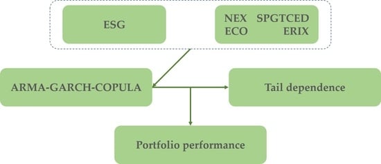
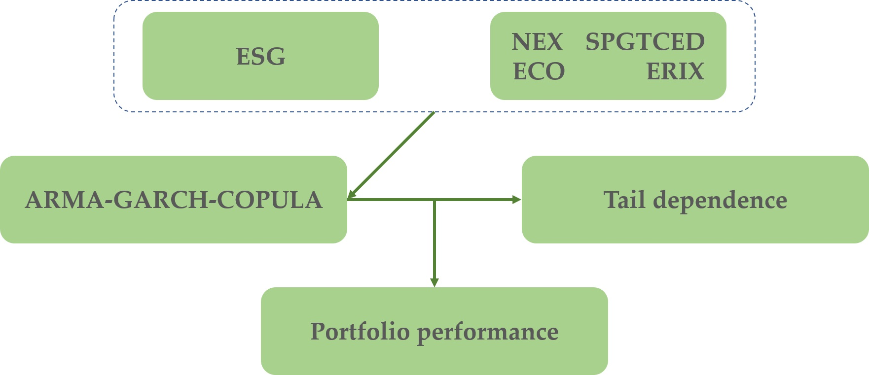
In this research, we first model the marginal distribution for the returns of each financial asset. Then, we use copula models to study the dependence between the ESG index and each of the energy stock indices. Four pairs are thus formed: ESG-NEX, ESG-ECO, ESG-SPGTCED, and ESG-EIRX. Finally, the portfolios of these four pairs will be discussed separately. In this section, we will discuss the marginal distribution models and copula theory. We use not only static copula models but also time varying ones.
2.1. Modeling Marginal Distributions
It is a well-known fact that financial assets have features such as fat tails and serial correlation. Fama supported both fat tailed and skewed distribution [18] in terms of the Mandelbrot stable Paretian distribution, i.e., a stable Levy distribution which was also pointed out in [19]. This can be overcome by using truncated Levy flight (TLF) distribution in [20]. Levy flights appear due to the presence of specific features of autocorrelation [21].
To model the daily returns of the ESG index and energy stock indices, we use the autoregressive moving average (ARMA) model and the standard generalized autoregressive conditional heteroscedasticity (GARCH (1,1)) model [22,23]. The orders of the ARMA and GARCH models are selected by the Bayesian Information Criterion (BIC). We denote the daily returns as the variable and the shocks as . The standard residual is an independent and identically distributed variable, having a zero mean and unit variance.
Before using the copula models to estimate the dependence on standard residuals, we need to transform into a uniform (0,1) distribution. Following Patton [24], we include both parametric (flexible skew t) and nonparametric (empirical distribution function, EDF) models in the transformation of standard residuals. The flexible skew t-model, developed by Hansen [25], has two coefficients, and . This model is preferred since it is flexible in estimating the normal, Student’s t, and skew t-distributions with the change of coefficients.
To ensure we estimate the marginal distribution effectively, several tests are carried out on the results. We use the Ljung–Box test to test if there is an autocorrelation within the (squared) standard residuals up to a chosen lag. The Kolmogorov–Smirnov (KS, Equation (5)) and Cramer Von–Mises (CvM, Equation (6)) tests are chosen for the goodness-of-fit test on the skew t model. We follow the simulation methods in the study of Genest and Rémillard [26] to provide the critical values for KS and CvM. Given the parameters in the marginal distribution models, we simulate S observations and again estimate the models based on the newly produced observations. Then, we compute the KS and CvM statistics and repeat the steps above for T times. The values in the upper order of the produced T statistics are used as the KS and CvM critical values, separately.
2.2. Copula Functions
Sklar [27] documented that one can obtain the decomposition of a joint distribution in n dimensions using marginal distributions and the copula function, the latter of which deals with uniform distributed variables. The copula model is a mature method of calculating the level of dependence, including various types of dependence in static and time varying ways. Theoretically, normal (Gaussian) copula can only observe correlations rather than tail dependences. In the Student’s t copula model, it is assumed that the tail dependences are symmetric. Models such as the Clayton and rotated Gumbel copula can obtain dependence in the lower tail. Furthermore, if we consider the copula parameters evolving over time, a copula model can be regarded as a time varying model and yield a time-varying level of dependence. In this research, we consider only copula models with two input variables, and . Further, we assume that and follow uniform distribution. The models used are given in Table 1. In a normal copula, possesses a univariate standard normal distribution, and represents a linear correlation coefficient. is used to denote the parameter in the Clayton and Gumbel copula [28] model, and dependence is calculated as . In this research, we use the rotated Gumbel copula by denoting a new rank in the uniform variables (i.e., we produce and ). The dependence is then calculated as . In the Student t copula, the parameter represents the degrees of freedom, and is the inverse of a standard Student’s t distribution.
2.3. Generalized Autoregressive Score (GAS) Model in Time Varying Copula
Among the five constant copula models, we select the rotated Gumbel copula and Student’s t copula models to further investigate the time varying dependence features. Recently, the generalized autoregressive score (GAS) model, introduced by Creal et al. [29], has been frequently used as a method for obtaining the time varying parameters in copula functions. We denote as the time-varying copula parameter. Similar to the GARCH model, another term is used to help describe the movement of the autoregressive parameter. The score of the likelihood is used as the information set. The implicit form of can be shown as . To ensure the movement does not go below 1, the parameter in the rotated Gumbel copula can be written as . Similarly, can be used in Student’s t copula to ensure the correlation parameter lies between −1 and 1.
where
3. Empirical Results
3.1. Summary Statistics
We collect data from Bloomberg database, from 28 September, 2007 to 16 April, 2019. In our research, we use the S&P 500 ESG index (the market capitalization-weighted index that measures the performance of securities meeting sustainability criteria) to represent numerous alternative ESG investments. Based on the variable selection of Reboredo [12], we choose four stock indices as our agents for the renewable energy global index.
- (1)
- The Wilder Hill New Energy Global Innovation Index (NEX (for more details on the weights of the NEX index, please refer to https://nexindex.com/whindexes.php.)) is weighted based on globally listed new energy innovation companies and is calculated by Solactive. The index focuses on renewable—solar (27.5% weight), renewable—wind (22.0% weight), energy conversion (5.5% weight), energy efficiency (23.1% weight), energy storage (6.6% weight), renewables—Biofuels % Biomass (8.8% weight), and renewables—others (6.6% weight).
- (2)
- The Wilder Hill Clean Energy Index (ECO (for more details on the weights of the ECO index, please refer to https://wildershares.com/about.php)) is mainly on US-listed clean energy companies and is calculated by the New York Stock Exchange (NYSE). The index focuses on renewable energy supplies (21% weight), energy conversion (21% weight), power delivery and conservation (20% weight), greener utilities (13% weight), energy storage (20% weight), and cleaner fuels (5% weight).
- (3)
- The S&P Global Clean Energy Index (SPGTCED (for more details on the weights of the SPGTCED index, please refer to https://us.spindices.com/indices/equity/sp-global-clean-energy-index)) is weighted based on 30 companies from around the world that are related to clean energy business. The index focuses largely, different from the other three indices, on information technology (24.6% weight). Other weights are allocated on utilities (52.4% weight), industrials (20.8% weight), and energy (2.1% weight).
- (4)
- The European Renewable Energy Total Return Index (ERIX (for more details on the weights of the ERIX index please refer to https://sgi.sgmarkets.com/en/index-details/TICKER:ERIX/)) tracks the stocks of largest European renewable energy companies that are highly involved in wind, water, solar, biofuels, geothermal, and/or marine investments. The index selects the largest companies, in which each component has a minimum weight of 5%. According to the most current weights, the companies are Verbund ag in Austria (21.75% weight), Vestas wind systems a/s in Denmark (20.52% weight), Siemens gamesa renewable ene in Spain (17.67% weight), Edp renovaveis sa in Spain (10.29% weight), and Meyer burger technology in Switzerland (5.95% weight).
Investors cannot directly buy indices but can invest in exchange-traded funds (ETFs), which mirror the indices introduced above. In this paper, we regard each index (or equivalent ETF) as an asset, so they all have prices and returns.
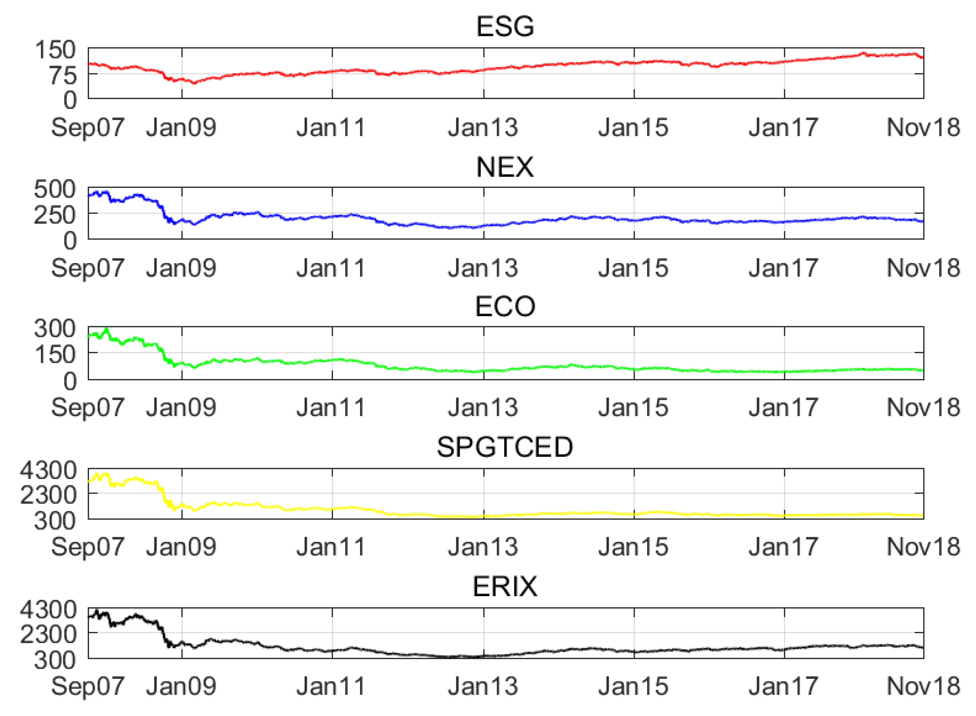
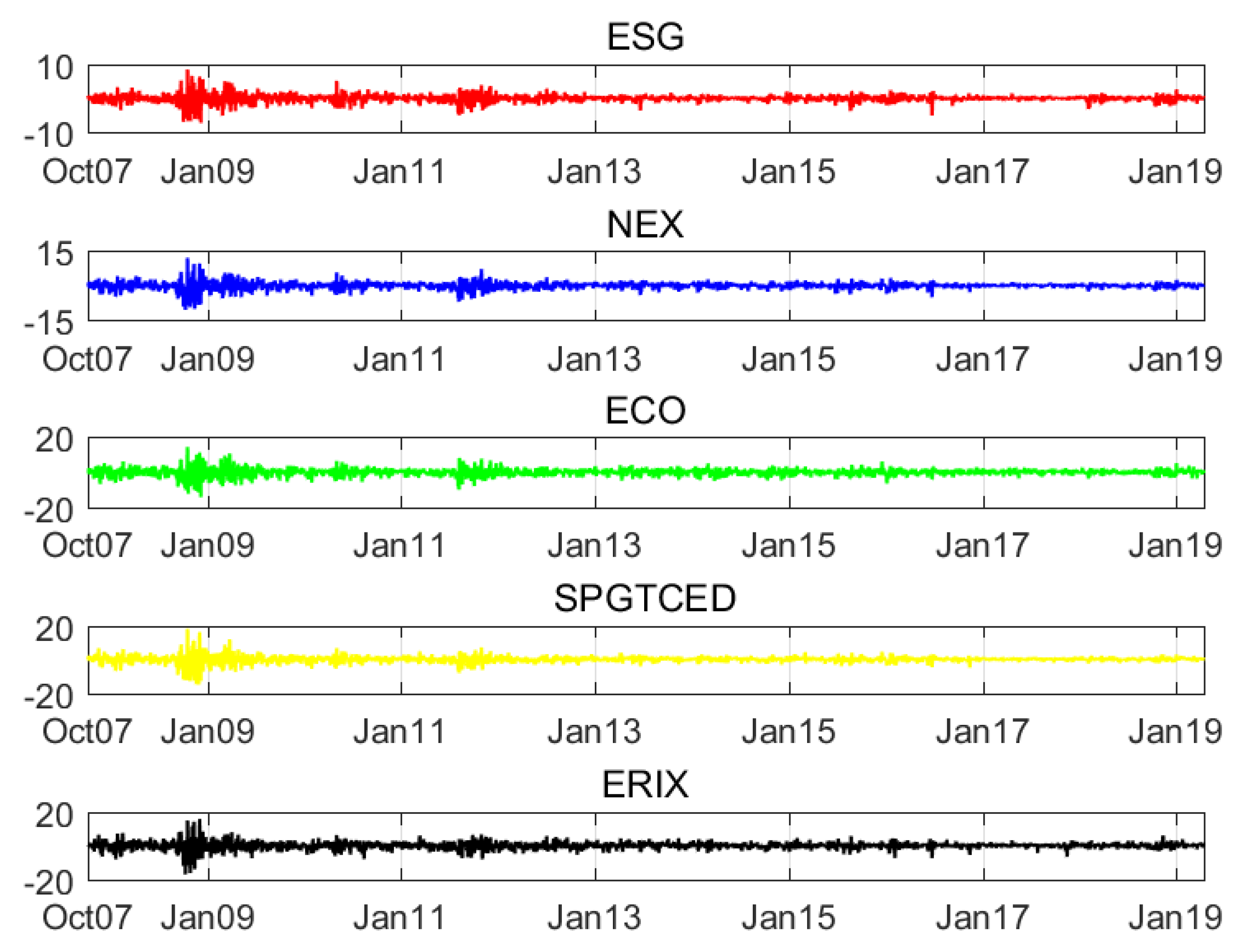
To obtain stationary time series data, we compute the first difference of the natural logarithm of asset prices by multiplying 100 as the returns shown as percentages. Descriptive statistics of the returns are provided in Table 2. Among the four financial assets, only the ESG index gain positive revenues, while the worst case for renewable energy index is negative 0.07% for the average return. In terms of the variation reflected by standard errors and extreme values, the ESG index experiences the lowest volatility. Left-skewed features are found in all assets, indicating a fat tail in the negative returns. The prices and returns of five assets are shown in Figure 1 and Figure 2, respectively. Cointegration and Granger causality between the ESG index and each of other three indices are tested (Table A1).
3.2. Results for the Marginal Distributions
The results for marginal distributions are shown in Table 3. In order to derive the marginal distributions, the ARMA model is estimated based on stock index returns. Furthermore, the standard GARCH model is estimated on the ARMA residuals to obtain the standard residuals. AR (2) is chosen for all stock indices returns according to the BIC criteria. Almost all coefficients in the standard GARCH model in the five returns are at a 1% significant level. The Ljung–Box test is applied, and the insignificant results document the non-autoregressive features (up to 25 lags) of the standard residuals, as well as the squared ones, at a 10% confidence level. As stated before, the skew t density model is used to model the standard residuals in the standard GARCH model before further calculation in the copula model. The degrees of freedom in the skewed t density model coincide with those from the standard GARCH model estimation. The goodness-of-fit test, including the Kolmogorov–Smirnov (KS) and Cramer Von–Mises (CvM) tests, yields insignificant statistics about the skew t distribution model. The skew t density model appropriately specifies the distribution of the standard residuals.
3.3. Results in the Copula Models
After estimating the AR-GARCH model, the standard residuals for each future return are transformed into a uniform marginal using the skewed t model and empirical distribution function (EDF) methods. Two probability integral transforms are called parametric and nonparametric models, respectively. With these transformed data, we estimate the parameters of various copula models. The constant copula models in this paper include the normal copula, Clayton copula, rotated Gumbel copula, and Student’s t copula. The normal copula model yields a correlation between the two series of data. The Clayton copula and rotated Gumbel copula results indicate the dependence of the lower tails between the two series of data. The Student’s t copula shows symmetrical dependence structures in the lower and upper tails.
The ESG index and the renewable energy stock indices yield four groups (portfolios) with corresponding dependence levels: ‘ESG and NEX’, ‘ESG and ECO’, ‘ESG and SPGTCED’, and ‘ESG and ERIX’. The results of the constant copula models are shown in Table 4. The rankings for the levels of dependence in the four groups are the same in the normal and Clayton copula, with the ‘ESG and NEX’ group being the highest and the ‘ESG and ERIX’ group being the lowest. In the results for Student’s t copula, the ‘ESG and SPGTCED’ rather than ‘ESG and ECO’ group is the second strongest in dependence.
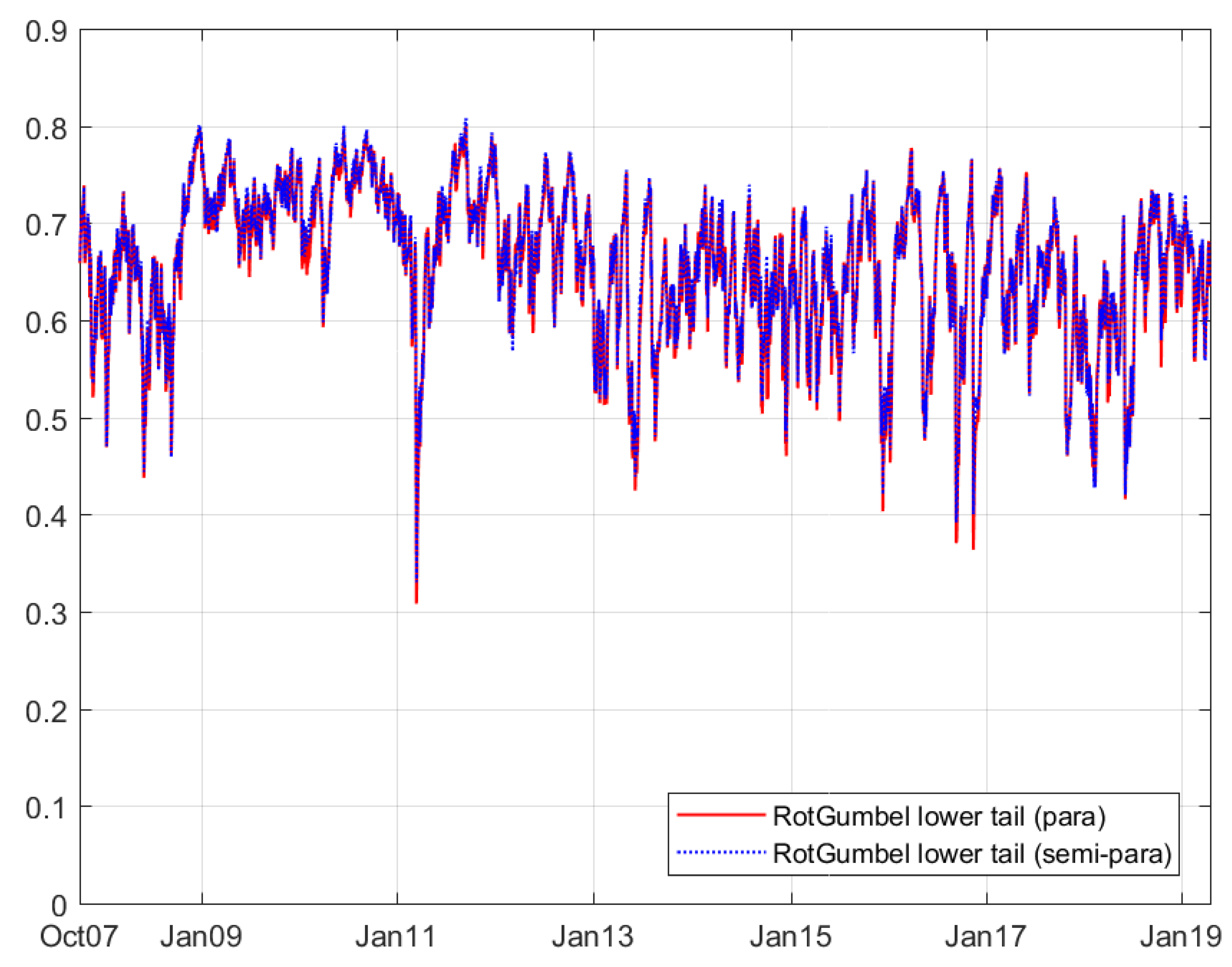
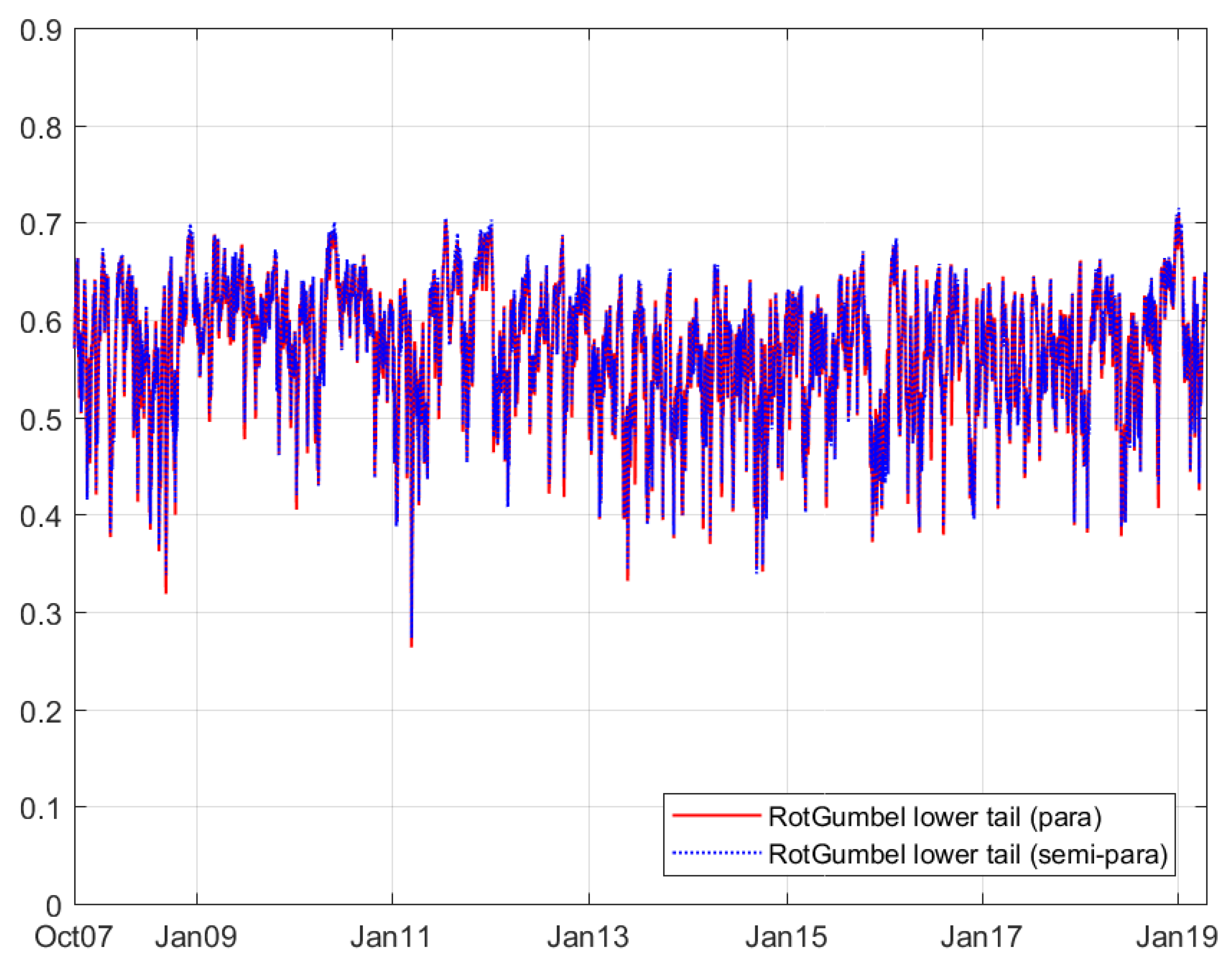
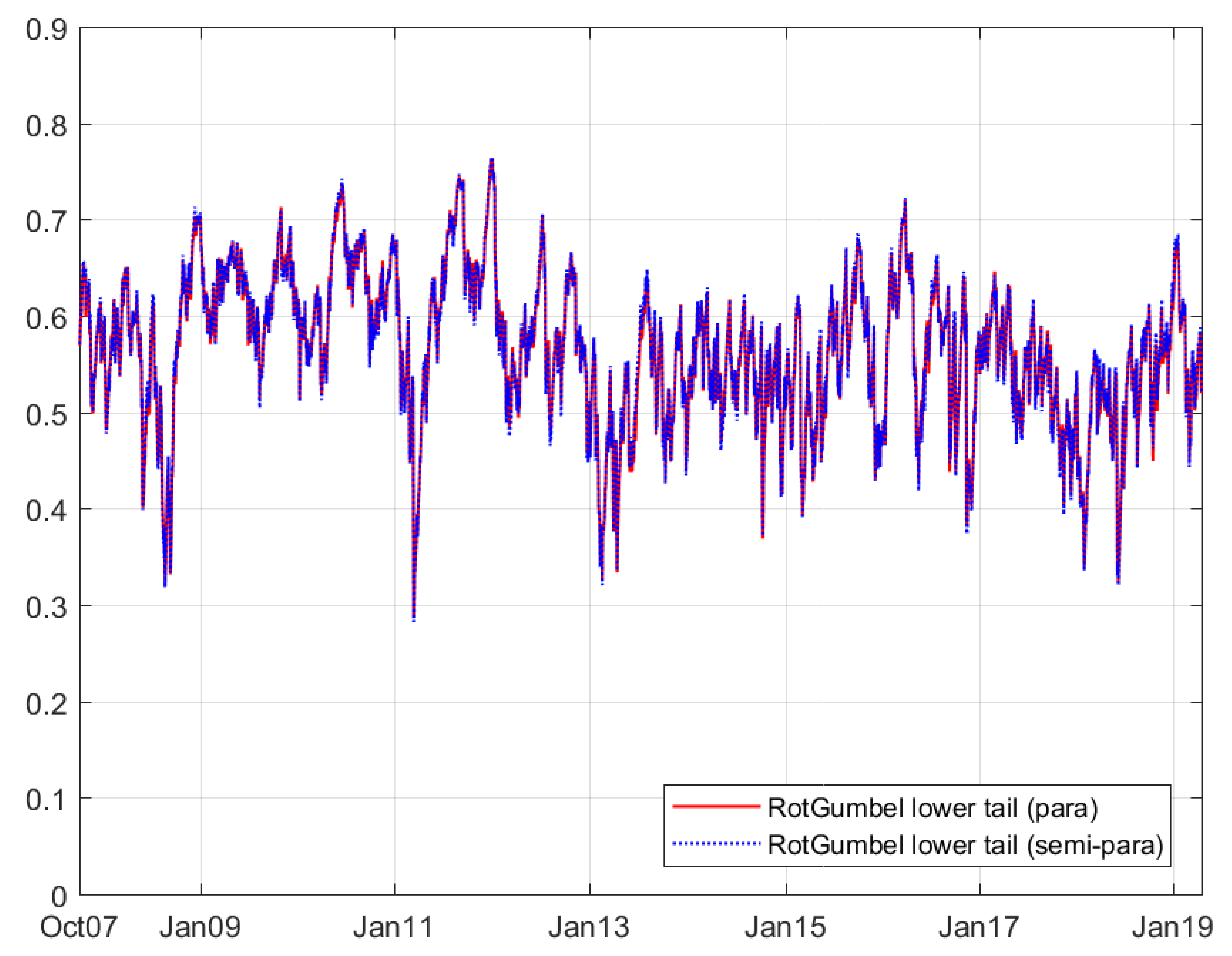
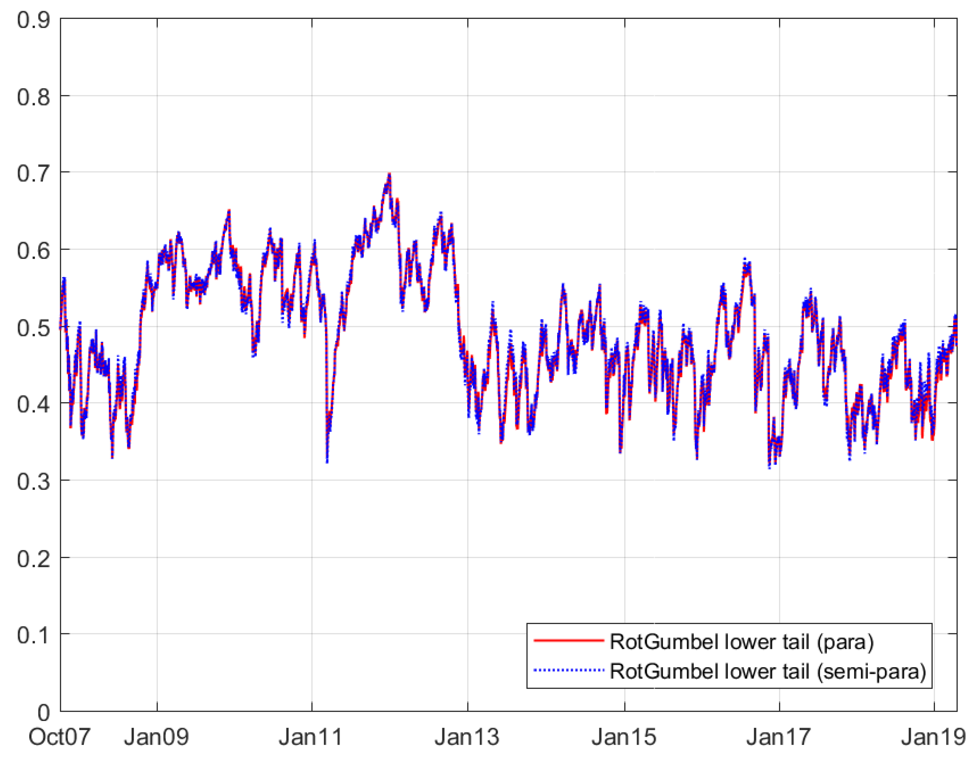
The results for the copula models with time variation are provided in Table 5. Detailed innovations are also presented in Figure 3, Figure 4, Figure 5 and Figure 6. The GAS model is used in the evolving model for the copula parameter. In four time-varying models, we select the student’s t rather than normal copula to better reflect the dependence on both sides. According to Patton [24], rotated Gumbel copula performs better than the Clayton family and they both measure the lower tail dependence; hence, we choose the Gumbel copula in time-varying case. The copula parameter in the next period will be based on the copula parameter in this period and the score of the copula-likelihood.
3.4. Goodness-of-Fit Test
In order to carry out the goodness-of-fit test for both the constant and time varying copula models, Kolomogorov–Smirnov and Cramer–von Mises methods are used in this paper. For the time varying copula models, the standard residuals should be transformed via the Rosenblatt method. In these two tests, significant statistics indicate that the models based on the data are rejected. The results of the tests on the constant and time varying copula models are reported in Table 6.
In the normal copula models, only the estimations of the parametric method pass the test. For the Clayton copula, no estimation passes the GOF test. For the rotated Gumbel copula, only one semi-parametric case passes the GOF test. For the Student’s t copula, only two estimations in semi-parametric cases yielded good results.
In time varying copula models, the p-values in the parametric case are higher than those in the semi-parametric case, although almost all combinations pass both copula models. Comparatively, time varying models under the GAS method offer a better fit for the data than that of the constant copula models.
4. Portfolio Performance
As shown above, we combine the ESG index with each of the renewable energy stock indices to form pairs and study their dependence structures. We further regard each pair of financial assets as a portfolio, each with different weights. By analyzing the traditional performance standards, such as risk adjusted returns and value-at-risk (VaR), market participators investing in renewable energy index funds and ESG can evaluate the potential revenues and stability behind each portfolio. We denote the portfolios between the ESG index and the renewable energy index as: ESG-NEX, ESG-ECO, ESG-SPGTCED, and ESG-EIRX. In this section, the skew t model and rotated Gumbel copula model will be used to estimate marginal distributions and dynamic dependence. In order to observe the performance of two financial assets, we first need to obtain the linear correlation so we can calculate the covariance and hence the portfolio variance. We simulated the correlation between the two returns using the copula parameters, as shown in Equation (8). Rather than analytically obtaining the results, we used a simulation based on the work by Patton [24].
where and denote different series.
We consider three types of weights for two financial assets. In this research, we denote as the ith type of weight in the ESG and as the weight in the renewable energy stock index at time t. It is assumed that there is no transaction cost, so frequent changes in dynamic weights are allowed and will not affect the returns. The first method involves allocating a constant weight in the ESG index. We regard the portfolio as a ‘static portfolio’. The second method (Equation (9)) is called ‘diversified risk-parity’, which provides greater capital in assets with less volatility. The third method (Equation (10)) is to consider the method developed by Kroner and Ng [30], which we regard as the ‘optimal portfolio’. The latter two dynamic weights are calculated based on conditional variance and covariance.
The potential performances, including conditional returns, variance, value-at-risk (VaR), and conditional value-at-risk (CVaR, which is also called as expected shortfall (ES)), are obtained based on the following steps. The portfolio contains two assets, denoted as and .
- We generate dynamic rotated Gumbel copula parameters based on the estimated time varying pattern.
- For time t from 1 to T (total sample size), we generate uniform distributions for two targets and using for S (= 5000) times, and hence the simulated standard residuals and returns based on the estimated marginal distribution parameters. Each element in marginal distributions at time t is stored in a vector of size .
- For time t, the portfolio returns are calculated based on each asset return and weight. For asset returns of size , a lower qth quantile (we selected 1%, indicating a confidence level of 99% for VaR) is regarded as the VaR (Equation (11)). CVaR can also be obtained (Equation (12)).
To decide whether the portfolio performs better under a given strategy, we introduce four performance measurements to compare the portfolio and original benchmark returns. Since we investigate the performance of reinforcement after putting the ESG index into the renewable energy index fund, the benchmark portfolio will only include the renewable energy index (i.e., ). The first measurement is the risk-adjusted returns (RR), indicating returns in units of standard deviation. This comparison requires a standardization of the benchmark (Equation (13)). ( is short for ‘comparison in ′) obtains the relative change of in the portfolio compared to in the benchmark. () yields results allowing the portfolio to acquire a higher (or lower) RR. The second measurement is to compare the standard deviation (SD) of the returns. Similar to , also requires standardization to show the relative changes. () indicates that the portfolio returns are more (less) stable. The third and fourth methods are used to measure the VaR (Equation (15)) and CVaR (ES) (Equation (16)), which are the key elements in portfolio risk management. We compare the portfolio with the benchmark at every time point before taking the average values. () demonstrates that the portfolio is more (or less) risky than the benchmark (normally we assume that and () have negative signs).
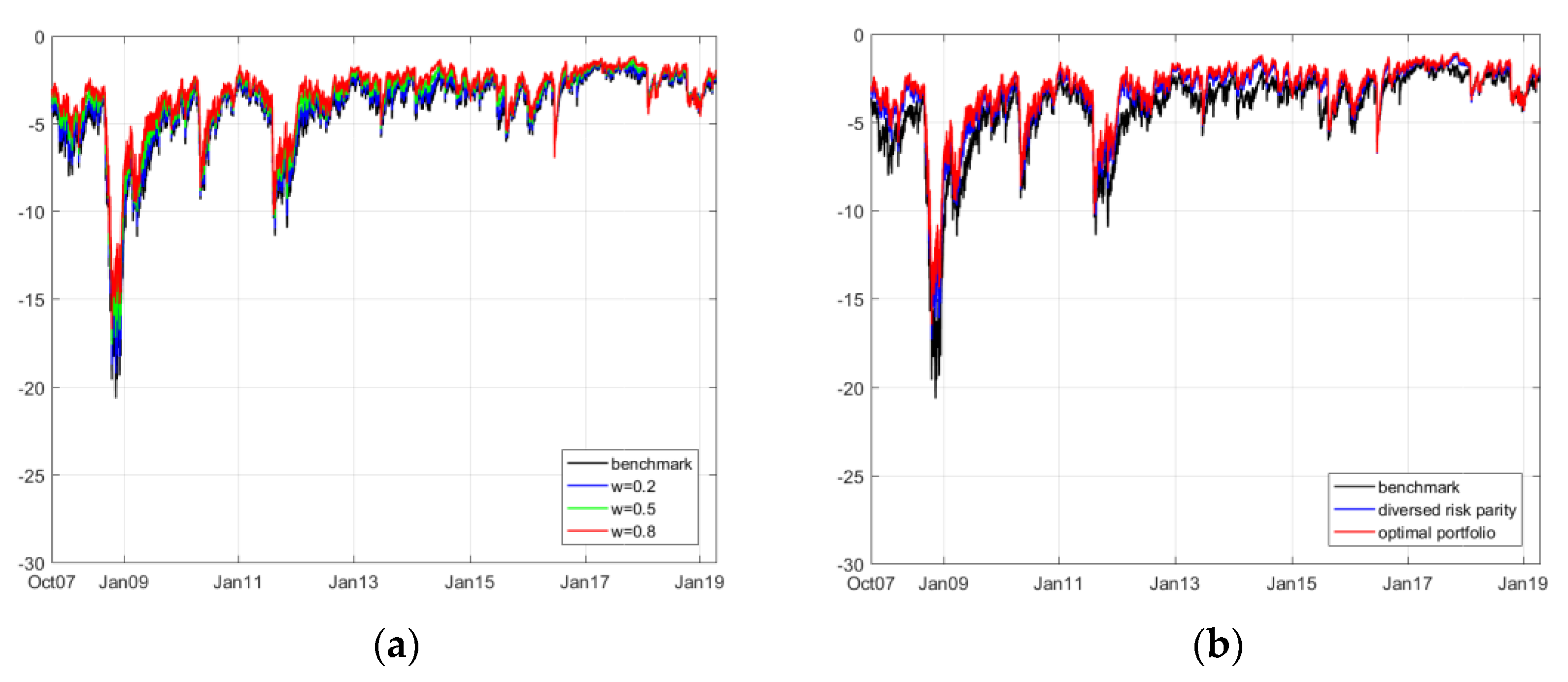
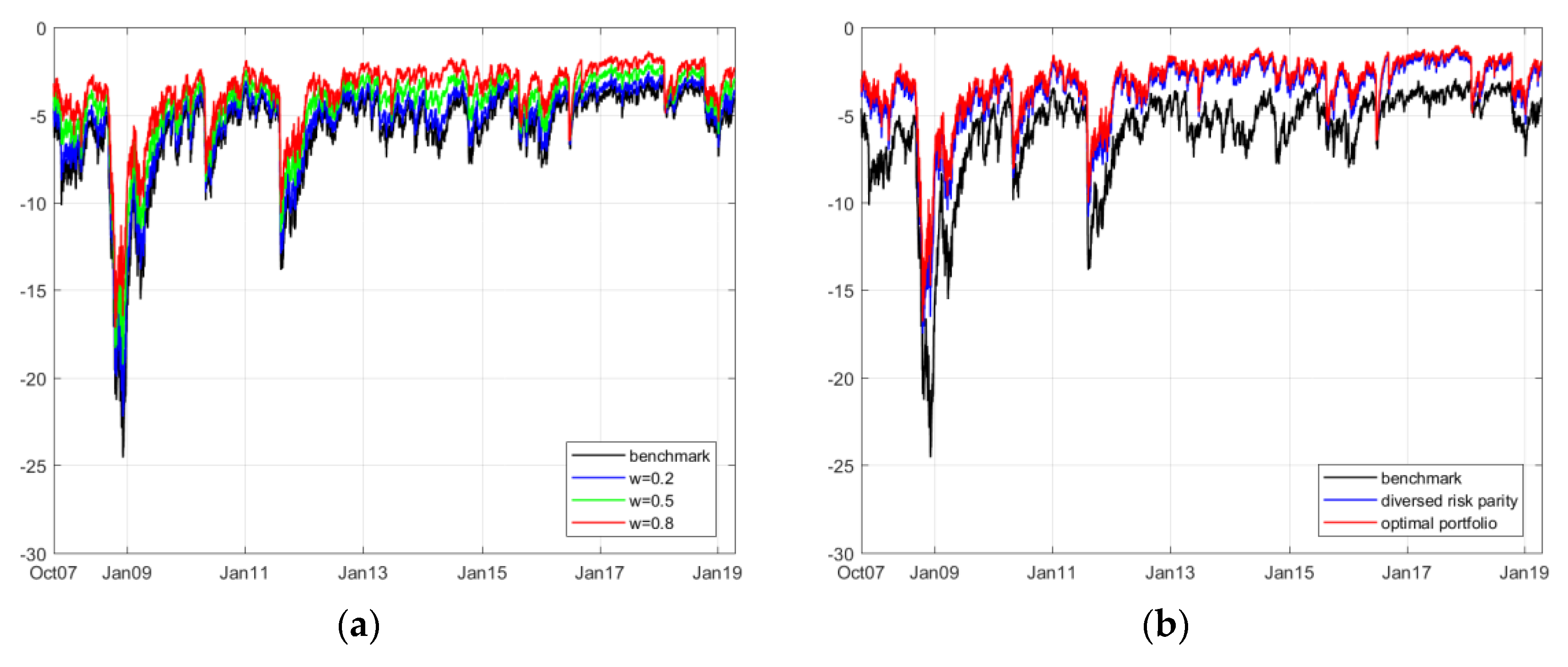
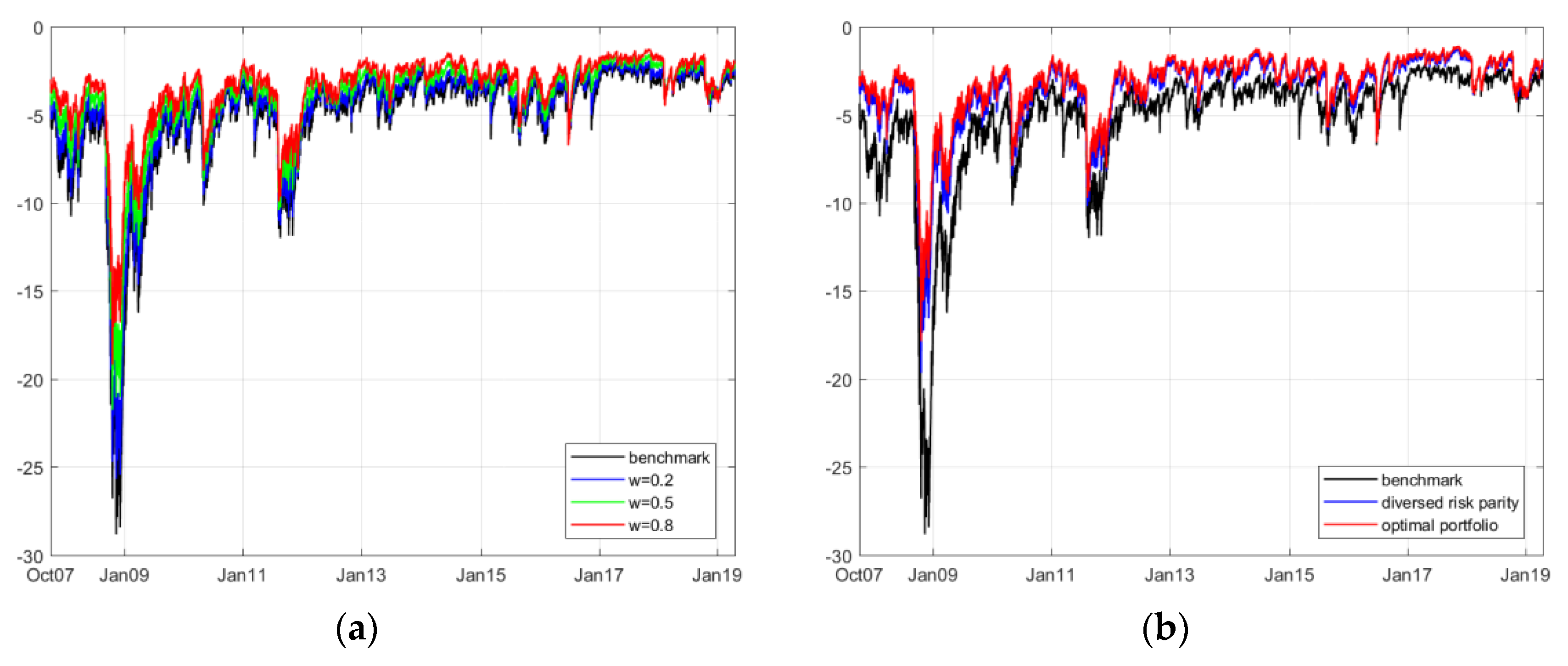
The results of the comparison between the portfolios under different weights and benchmarks are shown in Table 7. Furthermore, we provide the dynamic CVaR innovation of four different portfolios in Figure 7, Figure 8, Figure 9 and Figure 10.
The positive values in the comparison of the risk-adjusted returns indicate that the ESG index can increase the profitability level compared to merely investing in the renewable energy index. In the statistics for the returns in the indices listed above, we determine that only the ESG index yields positive revenue. It is thus reasonable that the ESG can increase the revenue in combined investments. Compared to the original status, the combination of ESG and SPGTCED increase the profitability at the highest level, followed closely by the group of ESG and NEX.
When we compare the standard deviation in all groups of investments, we conclude that the ESG index can effectively decrease the deviation of the constructed portfolios. In all forms of strategies, the combination of ESG and ERIX outperform other groups in vanishing volatility. The second-best combination of decreasing the volatility is the group of ESG and ECO. The main reason may be that the original standard deviation values of ERIX and ECO indices are the highest. Therefore, the vanished volatility is obvious.
The ESG index can effectively benefit the portfolios in lowering the value-at-risk level at a large scale. All renewable energy indices can reduce the value-at-risk level by at least 10%, 18%, and 25% under the Naïve static, diversified risk parity, and optimal weights strategies, respectively. In the case of ESG and ERIX, the VaR and CVaR (ES) levels yield the best results.
Thus, the ESG can help ERIX and ECO reduce standard deviation at the largest scale. The ESG and ERIX group is the most successful group in reducing the VaR and CVaR (ES) levels (at nearly 50% of their original levels). These results suggest that using the ESG index in the investment of the renewable energy index should be appealing to most fund managers.
5. Conclusions
The introduction of the ESG index facilitated the diversity of capital investment and fund management. Based on this research, we have studied the essential nature of portfolios and the dependence structure of numerous securities (ETF). The most common and traditional way to reduce the risk and increase the risk-adjusted return is to manage the potential linear correlation among returns. However, to compete in the fierce battlefield of fund management, fund managers need to further investigate the dependence structure in not only constant but also time-varying cases; hence, more precise performance can be simulated in the hypothetical portfolios. Our research, using the constant and time-varying copula models, can help fund managers predict the potential benefits gained from the ESG index if they consider putting the ESG index into the current renewable energy index. These benefits are reasonable since they are similar in topic, and, as stated before, the ESG index has decent historical performance and satisfactory applicability to companies.
Accordingly, we segment the detailed dependence structures into four groups and compare their performances compared with merely investing in the renewable energy index (as the current renewable energy index fund/ETF). Overall, the results suggest that we can trust the ESG index in hedging investment risk and increasing the profitability level in fund management. For example, in the case of investing in the ERIX index, the introduction of the ESG index can effectively reduce the potential value-at-risk level by as much as 50%; meanwhile, this index keeps the simulated revenue positive and more stable. During huge losses, such as the 2008 and 2011 crises, the time varying CVaR graphs reveal that balancing the renewable energy index with the ESG index can be helpful in reducing large losses.
Author Contributions
Conceptualization, S.H.; investigation, G.L.; writing—original draft preparation, G.L.; writing—review and editing, S.H.; project administration, S.H.; funding acquisition, S.H. All authors have read and agreed to the published version of the manuscript.
Funding
This work was supported by JSPS KAKENHI, grant number 17H00983.
Acknowledgments
We are grateful to three anonymous referees for their helpful comments and suggestions.
Conflicts of Interest
The authors declare no conflict of interest.
Appendix A

Table A1.
Portfolio cointegration and Granger causality test (p-value).
| Tests | ESG and NEX | ESG and ECO | ESG and SPGTCED | ESG and ERIX |
|---|---|---|---|---|
| Cointegration (index) | 0.9659 | 0.8583 | 0.8763 | 0.9660 |
| ESG → others (returns) | 0.0001 | 0.0102 | 0.0702 | 0.0001 |
| ESG ← others (returns) | 0.0001 | 0.0001 | 0.0111 | 0.0001 |
Notes: In this table, four pairs of index and returns are tested in Engle–Granger cointegration and causality. The maximum lag is set as 5. In the Granger causality test, A → B implies that A is the Granger cause of B, vise verse. We test the cointegration on originally daily index values, while testing the Granger causality on daily returns.
References
- Tang, D.Y.; Zhang, Y. Do shareholders benefit from green bonds? J. Corp. Financ. 2018. [Google Scholar] [CrossRef]
- Klassen, R.; McLaughlin, C. The impact of environmental management on frm performance. Manag. Sci. 1996, 42, 1199–1214. [Google Scholar] [CrossRef]
- Mello, A.S.; Parsons, J.E. Hedging and Liquidity. Rev. Financ. Stud. 2000, 13, 127–153. [Google Scholar] [CrossRef] [Green Version]
- Lins, K.V.; Servaes, H.; Tufano, P. What drives corporate liquidity? An international survey of cash holdings and lines of credit. J. Financ. Econ. 2010, 98, 160–176. [Google Scholar] [CrossRef]
- Shin, Y.J.; Pyo, U. Liquidity Hedging with Futures and Forward Contracts. Stud. Econ. Financ. 2019, 36, 265–290. [Google Scholar] [CrossRef]
- Kaminker, C.; Stewart, F. “The Role of Institutional Investors in Financing Clean Energy OECD Working Papers on Finance, Insurance and Private Pensions, No.23, OECD Publishing.” 23. OECD Working Papers on Finance, Insurance and Private Pensions. 2012. Available online: www.oecd.org/daf/fin/wp (accessed on 1 September 2019).
- Dimson, E.; Karakaş, O.; Li, X. Active ownership. Rev. Financ. Stud. 2015, 28, 3225–3268. [Google Scholar] [CrossRef] [Green Version]
- Hoepner, A.; Oikonomou, I.; Sautner, Z.; Starks, L.; Zhou, X. ESG Shareholder Engagement and Downside Risk. Unpublished work. 2018. [Google Scholar]
- Sultana, S.; Zulkifli, N.; Zainal, D. Environmental, Social and Governance (ESG) and Investment Decision in Bangladesh. Sustainability 2018, 10, 1831. [Google Scholar] [CrossRef] [Green Version]
- Keppler, J.H.; Mansanet-Bataller, M. Causalities between CO2, electricity, and other energy variables during phase I and phase II of the EU ETS. Energy Policy 2010, 38, 3329–3341. [Google Scholar] [CrossRef] [Green Version]
- Reboredo, J.C.; Rivera-Castro, M.A.; Ugolini, A. Wavelet-based test of co-movement and causality between oil and renewable energy stock prices. Energy Econ. 2017, 61, 241–252. [Google Scholar] [CrossRef]
- Reboredo, J.C. Is there dependence and systemic risk between oil and renewable energy stock prices? Energy Econ. 2015, 48, 32–45. [Google Scholar] [CrossRef]
- Rockafellar, R.T.; Uryasev, S. Optimization of Conditional Value-at-Risk. J. Risk 2000, 2, 21–41. [Google Scholar] [CrossRef] [Green Version]
- Pflug, G.C. Some remarks on the value-at-risk and the conditional value-at-risk. In Probabilistic Constrained Optimization; Springer: Boston, MA, USA, 2000; pp. 272–281. [Google Scholar]
- Artzner, P.; Delbaen, F.; Eber, J.M.; Heath, D. Coherent measures of risk. Math. Financ. 1999, 9, 203–228. [Google Scholar] [CrossRef]
- Deng, L.; Ma, C.; Yang, W. Portfolio optimization via pair copula-GARCH-EVT-CVaR model. Syst. Eng. Procedia 2011, 2, 171–181. [Google Scholar] [CrossRef] [Green Version]
- He, X.; Gong, P. Measuring the coupled risks: A copula-based CVaR model. J. Comput. Appl. Math. 2009, 223, 1066–1080. [Google Scholar] [CrossRef] [Green Version]
- Fama, E.F. The behavior of stock-market prices. J. Bus. 1965, 38, 34–105. [Google Scholar] [CrossRef]
- Hsu, D.A.; Miller, R.B.; Wichern, D.W. On the stable Paretian behavior of stock-market prices. J. Am. Stat. Assoc. 1974, 69, 108–113. [Google Scholar] [CrossRef]
- Mantegna, R.N.; Stanley, H.E. Introduction to Econophysics: Correlations and Complexity in Finance; Cambridge University Press: Cambridge, UK, 2000. [Google Scholar]
- Figueiredo, A.; Gleria, I.; Matsushita, R.; Da Silva, S. On the origins of truncated Lévy flights. Phys. Lett. A 2003, 315, 51–60. [Google Scholar] [CrossRef] [Green Version]
- Yang, L.; Hamori, S. Dependence structure among international stock markets: A GARCH-copula analysis. Appl. Financ. Econ. 2013, 23, 1805–1817. [Google Scholar] [CrossRef]
- Yang, L.; Hamori, S. Dependence Structure between CEEC-3 and German Government Securities Markets. J. Int. Financ. Mark. Inst. Money 2014, 29, 109–125. [Google Scholar] [CrossRef]
- Patton, A. Copula methods for forecasting multivariate time series. In Handbook of Economic Forecasting; Elsevier: Amsterdam, The Netherlands, 2013; Volume 2, pp. 899–960. [Google Scholar] [CrossRef]
- Hansen, B.E. Autoregressive conditional density estimation. Int. Econ. Rev. 1994, 35, 705–730. [Google Scholar] [CrossRef]
- Genest, C.; Rémillard, B. Validity of the parametric bootstrap for goodness-of-fit testing in semiparametric models. In Annales de l’Institut Henri Poincaré, Probabilités et Statistiques; Institut Henri Poincaré: Paris, France, 2008; Volume 44, pp. 1096–1127. [Google Scholar]
- Sklar, M. Fonctions de répartition à n dimensions et leurs marges. Publ. l’Inst. Stat. l’Univ. Paris 1959, 8, 229–231. [Google Scholar]
- Gumbel, E.J. Bivariate exponential distributions. J. Am. Stat. Assoc. 1960, 55, 698–707. [Google Scholar] [CrossRef]
- Creal, D.; Koopman, S.J.; Lucas, A. Generalized autoregressive score models with applications. J. Appl. Econom. 2013, 28, 777–795. [Google Scholar] [CrossRef] [Green Version]
- Kroner, K.F.; Ng, V.K. Modeling asymmetric comovements of asset returns. Rev. Financ. Stud. 1998, 11, 817–844. [Google Scholar] [CrossRef]
Figure 1.
Daily prices of the five assets from 28 September 2007 to 16 April 2019.

Figure 2.
Daily returns of the five assets from 28 September 2007 to 16 April 2019.

Figure 3.
Time varying lower tail dependence between ESG and NEX based on the rotated Gumbel copula (GAS) model.
Figure 3.
Time varying lower tail dependence between ESG and NEX based on the rotated Gumbel copula (GAS) model.

Figure 4.
Time varying lower tail dependence between ESG and ECO based on the rotated Gumbel copula (GAS) model.
Figure 4.
Time varying lower tail dependence between ESG and ECO based on the rotated Gumbel copula (GAS) model.

Figure 5.
Time varying lower tail dependence between ESG and SPGTCED based on the rotated Gumbel copula (GAS) model.
Figure 5.
Time varying lower tail dependence between ESG and SPGTCED based on the rotated Gumbel copula (GAS) model.

Figure 6.
Time varying lower tail dependence between ESG and ERIX based on the rotated Gumbel copula (GAS) model.
Figure 6.
Time varying lower tail dependence between ESG and ERIX based on the rotated Gumbel copula (GAS) model.

Figure 7.
Time varying conditional value-at-risk (CVaR) between the ESG and NEX portfolios ((a) is the CVaR under the ‘naïve static’ strategy; (b) is the CVaR under the ‘diversified risk parity’ and ‘optimal weights’ strategies).
Figure 7.
Time varying conditional value-at-risk (CVaR) between the ESG and NEX portfolios ((a) is the CVaR under the ‘naïve static’ strategy; (b) is the CVaR under the ‘diversified risk parity’ and ‘optimal weights’ strategies).

Figure 8.
Time varying CVaR between the ESG and ECO portfolios ((a) is the CVaR under the ‘naïve static’ strategy; (b) is the CVaR under the ‘diversified risk parity’ and ‘optimal weights’ strategies).
Figure 8.
Time varying CVaR between the ESG and ECO portfolios ((a) is the CVaR under the ‘naïve static’ strategy; (b) is the CVaR under the ‘diversified risk parity’ and ‘optimal weights’ strategies).

Figure 9.
Time varying CVaR between the ESG and SPGTCED portfolios ((a) is the CVaR under the ‘naïve static’ strategy; (b) is the CVaR under the ‘diversified risk parity’ and ‘optimal weights’ strategies).
Figure 9.
Time varying CVaR between the ESG and SPGTCED portfolios ((a) is the CVaR under the ‘naïve static’ strategy; (b) is the CVaR under the ‘diversified risk parity’ and ‘optimal weights’ strategies).

Figure 10.
Time varying CVaR between the ESG and ERIX portfolios ((a) is the CVaR under the ‘naïve static’ strategy; (b) is the CVaR under the ‘diversified risk parity’ and ‘optimal weights’ strategies).
Figure 10.
Time varying CVaR between the ESG and ERIX portfolios ((a) is the CVaR under the ‘naïve static’ strategy; (b) is the CVaR under the ‘diversified risk parity’ and ‘optimal weights’ strategies).

Table 1.
Copula functions.
| Copula Family | Name |
|---|---|
| Normal | |
| Clayton | |
| Gumbel | |
| Student t |
Notes: The empirical lower tail dependence of the Clayton copula and rotated Gumbel copula are calculated by and . Both tail dependences of the Student’s t-copula were calculated by . See Patton [24] for details on the copula functions.
Table 2.
Descriptive statistics of the returns of five financial assets.
| Mean | S.E. | Min | Max | Skewness | Kurtosis | Jarque–Bera | |
|---|---|---|---|---|---|---|---|
| ESG | 0.0040 | 1.0701 | −7.2143 | 8.5659 | −0.4448 | 11.6885 | 8837 |
| NEX | −0.0378 | 1.4811 | −10.4854 | 12.0705 | −0.4905 | 11.6112 | 8702 |
| ECO | −0.0654 | 2.1128 | −14.4673 | 14.5195 | −0.3655 | 8.2339 | 3236 |
| SPGTCED | −0.0706 | 1.9516 | −14.9729 | 18.0927 | −0.5195 | 16.6587 | 21733 |
| ERIX | −0.0474 | 2.1309 | −16.9652 | 15.8214 | −0.3927 | 11.2607 | 7977 |
Notes: This table summarizes the descriptive statistics of daily returns ranging from 28 September, 2007 to 16 April, 2019 with 2775 observations. ESG, NEX, ECO, SPGTCED, and ERIX are used to represent the S&P 500 ESG index, the Wilder Hill New Energy Global Innovation Index, the Wilder Hill Clean Energy Index, the S&P Global Clean Energy Index, and the European Renewable Energy Total Return Index, separately. The returns of the five assets show negative skewness around zero, large kurtosis, and Jarque–Bera statistics significant at 1%, indicating non-normal distributions.
Table 3.
Marginal distributions.
| ESG | NEX | ECO | SPGTCED | ERIX | |
|---|---|---|---|---|---|
| Mean Model | |||||
| 0.0547 *** | 0.0358 * | 0.0138 | 0.0111 | 0.0486 | |
| S.E. | (0.0129) | (0.0212) | (0.0312) | (0.0249) | (0.0295) |
| 0.1073 *** | 0.1934 *** | 0.0501 *** | 0.1410 *** | 0.0381 ** | |
| S.E. | (0.0192) | (0.0193) | (0.0195) | (0.0195) | (0.0192) |
| −0.0241 | −0.0026 | 0.0260 | 0.0068 | 0.0201 | |
| S.E. | (0.0195) | (0.0194) | (0.0195) | (0.0193) | (0.0192) |
| Variance Model | |||||
| 0.0070 *** | 0.0075 ** | 0.0383 *** | 0.0140 * | 0.0316 * | |
| S.E. | (0.0025) | (0.0034) | (0.0136) | (0.0055) | (0.0131) |
| 0.1067 *** | 0.0738 *** | 0.0741 *** | 0.0727 *** | 0.0721 *** | |
| S.E. | (0.0151) | (0.0116) | (0.0118) | (0.0119) | (0.0125) |
| 0.8923 *** | 0.9239 *** | 0.9160 *** | 0.9231 *** | 0.9219 *** | |
| S.E. | (0.0139) | (0.0115) | (0.0134) | (0.0120) | (0.0135) |
| 6.2547 *** | 8.6623 *** | 11.6211 *** | 8.2568 *** | 6.7693 *** | |
| S.E. | (0.7348) | (1.3224) | (2.3456) | (1.2253) | (0.8643) |
| Skewed t Density | |||||
| 6.5835 | 9.5779 | 12.6029 | 8.8251 | 7.0098 | |
| −0.1340 | −0.1138 | −0.1813 | −0.1044 | −0.0999 | |
| Ljung–Box Test | |||||
| 21.20 | 14.16 | 11.30 | 21.82 | 23.79 | |
| p value | (0.68) | (0.96) | (0.99) | (0.65) | (0.53) |
| 25.15 | 27.32 | 32.40 | 18.03 | 20.23 | |
| p value | (0.45) | (0.34) | (0.15) | (0.84) | (0.73) |
| GoF Tests on Skewed t Distribution Model (p-Value) | |||||
| KS | 0.30 | 0.68 | 0.84 | 0.17 | 0.31 |
| CvM | 0.34 | 0.32 | 0.72 | 0.15 | 0.30 |
Notes: This table provides the coefficients of the AR (2)-GARCH (1,1) model for each return. The standard errors for each parameter are reported in parentheses. ***, **, and * represent significance levels of 1%, 5%, and 10%, respectively. The skewness and degrees of freedom parameters are provided in the skew t model estimation. In the Ljung–Box test, the () statistics and p-values in parentheses are reported, showing that there is no autocorrelation in (squared) standard residuals up to 25 lags. The results of the goodness-of-fit test (GOF) on the skewed t model are provided as p-values. The null hypothesis of the GOF test (based on 1000 simulations) shows that the data follow the specified skewed t distribution, while the alternative hypothesis is that the data do not follow the specified skewed t distribution. A Cramer Von–Mises (CvM) test is usually regarded as a refinement of the Kolmogorov–Smirnov (KS) test.
Table 4.
Constant copula estimations.
| ESG and NEX | ESG and ECO | ESG and SPGTCED | ESG and ERIX | |||||
|---|---|---|---|---|---|---|---|---|
| Parametric | Semi | Parametric | Semi | Parametric | Semi | Parametric | Semi | |
| Normal Copula | ||||||||
| 0.7931 | 0.7933 | 0.6961 | 0.6951 | 0.6887 | 0.6887 | 0.6159 | 0.6159 | |
| S.E. | 0.0073 | 0.0075 | 0.0095 | 0.0111 | 0.0094 | 0.0100 | 0.0115 | 0.0127 |
| Log Likelihood | 1375.56 | 1377.16 | 919.51 | 915.75 | 892.20 | 892.21 | 661.72 | 661.68 |
| Clayton Copula | ||||||||
| 2.0344 | 2.0684 | 1.4834 | 1.4972 | 1.4452 | 1.4601 | 1.0640 | 1.0804 | |
| S.E. | 0.0586 | 0.0862 | 0.0633 | 0.0618 | 0.0611 | 0.0591 | 0.0510 | 0.0570 |
| 0.7113 | 0.7153 | 0.6267 | 0.6294 | 0.6190 | 0.6221 | 0.5213 | 0.5265 | |
| Log Likelihood | 1204.85 | 1227.97 | 861.37 | 865.30 | 816.19 | 827.34 | 564.71 | 571.87 |
| Rotated Gumbel Copula | ||||||||
| 2.3606 | 2.3754 | 1.9396 | 1.9434 | 1.9357 | 1.9401 | 1.6934 | 1.6984 | |
| S.E. | 0.0435 | 0.0472 | 0.0377 | 0.0313 | 0.0441 | 0.0386 | 0.0307 | 0.0314 |
| 0.6587 | 0.6612 | 0.5704 | 0.5714 | 0.5694 | 0.5706 | 0.4942 | 0.4960 | |
| Log Likelihood | 1400.45 | 1415.23 | 963.50 | 963.81 | 941.20 | 946.61 | 662.66 | 666.58 |
| Student’s t Copula | ||||||||
| 0.7986 | 0.7993 | 0.6997 | 0.6996 | 0.7000 | 0.7005 | 0.6228 | 0.6239 | |
| S.E. | 0.0085 | 0.0091 | 0.0116 | 0.0122 | 0.0120 | 0.0111 | 0.0149 | 0.0121 |
| 0.1637 | 0.1684 | 0.1340 | 0.1373 | 0.1789 | 0.1810 | 0.1261 | 0.1270 | |
| S.E. | 0.0234 | 0.0252 | 0.0192 | 0.0243 | 0.0204 | 0.0240 | 0.0217 | 0.0273 |
| 0.4014 | 0.4085 | 0.2544 | 0.2597 | 0.3187 | 0.3218 | 0.1838 | 0.1859 | |
| Log Likelihood | 1429.05 | 1432.08 | 948.61 | 945.42 | 954.46 | 953.46 | 691.27 | 691.08 |
Notes: In this table, the estimated coefficients and the standard errors obtained in the simulation with 100 bootstraps are reported. “Parametric” and “Semi” represent the parametric and semi-parametric models, respectively. The parameter boundaries of the normal copula, Clayton copula, rotated Gumbel copula, Student’s t copula, and SJC copula are set as , , , , and respectively. In our MATLAB code, the lower bound of the coefficient in the rotated Gumbel copula is set to be 1.1. The log likelihood values are reported using positive signs.
Table 5.
Time-varying copula estimations.
| ESG and NEX | ESG and ECO | ESG and SPGTCED | ESG and ERIX | |||||
|---|---|---|---|---|---|---|---|---|
| Parametric | Semi | Parametric | Semi | Parametric | Semi | Parametric | Semi | |
| Rotated Gumbel Copula (GAS) | ||||||||
| 0.0139 | 0.0146 | −0.0092 | −0.0078 | −0.0035 | −0.0037 | −0.0043 | −0.0042 | |
| S.E. | 0.0123 | 0.0151 | 0.0152 | 0.0088 | 0.0092 | 0.0115 | 0.0376 | 0.0593 |
| 0.1364 | 0.1371 | 0.1790 | 0.1720 | 0.0966 | 0.1015 | 0.0545 | 0.0543 | |
| S.E. | 0.0329 | 0.0569 | 0.0287 | 0.0528 | 0.0335 | 0.0631 | 0.0329 | 0.0492 |
| 0.9522 | 0.9522 | 0.8588 | 0.8750 | 0.9685 | 0.9663 | 0.9899 | 0.9899 | |
| S.E. | 0.1367 | 0.0384 | 0.1170 | 0.0253 | 0.1346 | 0.0258 | 0.1413 | 0.1108 |
| Log Likelihood | 1469.21 | 1485.20 | 992.11 | 992.89 | 983.49 | 989.66 | 697.50 | 702.23 |
| Student’s t Copula (GAS) | ||||||||
| 0.0480 | 0.0507 | 0.1236 | 0.1212 | 0.0862 | 0.0829 | 0.0109 | 0.0109 | |
| S.E. | 0.0219 | 0.0225 | 0.0421 | 0.0373 | 0.0280 | 0.0278 | 0.0132 | 0.0125 |
| 0.0921 | 0.0984 | 0.1328 | 0.1331 | 0.1354 | 0.1370 | 0.0442 | 0.0442 | |
| S.E. | 0.0146 | 0.0146 | 0.0245 | 0.0196 | 0.0184 | 0.0215 | 0.0115 | 0.0092 |
| 0.9782 | 0.9770 | 0.9288 | 0.9301 | 0.9501 | 0.9518 | 0.9926 | 0.9926 | |
| S.E. | 0.0101 | 0.0103 | 0.0243 | 0.0216 | 0.0157 | 0.0160 | 0.0087 | 0.0081 |
| 0.1154 | 0.1281 | 0.1185 | 0.1206 | 0.1467 | 0.1438 | 0.1108 | 0.1108 | |
| S.E. | 0.0206 | 0.0249 | 0.0201 | 0.0238 | 0.0223 | 0.0246 | 0.0216 | 0.0213 |
| Log Likelihood | 1499.70 | 1501.32 | 982.72 | 979.94 | 1002.50 | 1002.36 | 730.02 | 730.04 |
Notes: In this table, the estimated coefficients and standard errors obtained in the simulation with 100 bootstraps are reported. “Parametric” and “Semi” represent the parametric and semi-parametric models, respectively. Log likelihood values are reported using positive signs.
Table 6.
Goodness-of-fit test on the copula models.
| ESG and NEX | ESG and ECO | ESG and SPGTCED | ESG and ERIX | |||||
|---|---|---|---|---|---|---|---|---|
| Normal Copula | ||||||||
| Parametric | 0.28 | 0.25 | 0.23 | 0.11 | 0.17 | 0.17 | 0.26 | 0.26 |
| Semi | 0.02 | 0.01 | 0.01 | 0.01 | 0.01 | 0.01 | 0.04 | 0.01 |
| Clayton Copula | ||||||||
| Parametric | 0.01 | 0.02 | 0.01 | 0.04 | 0.01 | 0.02 | 0.02 | 0.02 |
| Semi | 0.01 | 0.01 | 0.01 | 0.01 | 0.01 | 0.01 | 0.01 | 0.01 |
| Rotated Gumbel Copula | ||||||||
| Parametric | 0.28 | 0.21 | 0.58 | 0.30 | 0.27 | 0.13 | 0.21 | 0.07 |
| Semi | 0.02 | 0.01 | 0.16 | 0.03 | 0.01 | 0.01 | 0.01 | 0.01 |
| Student’s t Copula | ||||||||
| Parametric | 0.26 | 0.34 | 0.35 | 0.09 | 0.10 | 0.15 | 0.36 | 0.29 |
| Semi | 0.03 | 0.01 | 0.01 | 0.01 | 0.03 | 0.01 | 0.13 | 0.01 |
| Rotated Gumbel Copula (GAS) | ||||||||
| Parametric | 0.01 | 0.01 | 0.99 | 0.99 | 0.99 | 0.99 | 0.01 | 0.01 |
| Semi | 0.42 | 0.86 | 0.99 | 0.99 | 0.99 | 0.99 | 0.54 | 0.41 |
| Student’s t Copula (GAS) | ||||||||
| Parametric | 0.41 | 0.20 | 0.47 | 0.22 | 0.11 | 0.08 | 0.16 | 0.21 |
| Semi | 0.06 | 0.01 | 0.01 | 0.01 | 0.02 | 0.01 | 0.01 | 0.01 |
Notes: This table shows the results of the Kolomogorov–Smirnov ) and Cramer–von Mises () tests on constant copula models of the standard residuals. The and methods test the time varying copula model of the Rosenblatt transform of the standard residuals. P-values that are smaller than 5% are shown in bold font. All results are based on 100 simulations.
Table 7.
Portfolio performance comparison.
| Strategy | Measure | ESG and NEX | ESG and ECO | ESG and SPGTCED | ESG and ERIX |
|---|---|---|---|---|---|
| Naïve Static | 0.0118 | 0.0106 | 0.0130 | 0.0078 | |
| −0.1672 | −0.2871 | −0.2640 | −0.2976 | ||
| −0.1404 | −0.2680 | −0.2406 | −0.2851 | ||
| −0.1364 | −0.2562 | −0.2070 | −0.2770 | ||
| Diversified risk parity | 0.0167 | 0.0237 | 0.0254 | 0.0159 | |
| −0.2066 | −0.4189 | −0.3777 | −0.4316 | ||
| −0.1852 | −0.4244 | −0.3379 | −0.4460 | ||
| −0.1801 | −0.4039 | −0.2986 | −0.4305 | ||
| Optimal weights | 0.0291 | 0.0345 | 0.0403 | 0.0267 | |
| −0.2722 | −0.4890 | −0.4502 | −0.4957 | ||
| −0.2501 | −0.4964 | −0.4052 | −0.5084 | ||
| −0.2389 | −0.4712 | −0.3615 | −0.4903 |
Notes: In this table, four comparative measurements of the performance between each portfolio and benchmark are reported. For the Naïve Static strategy, we only report the equally (50% to 50%) weighted examples. In each strategy, we report the best results in each row for , , and in bold font.
© 2020 by the authors. Licensee MDPI, Basel, Switzerland. This article is an open access article distributed under the terms and conditions of the Creative Commons Attribution (CC BY) license (http://creativecommons.org/licenses/by/4.0/).
Share and Cite
MDPI and ACS Style
Liu, G.; Hamori, S. Can One Reinforce Investments in Renewable Energy Stock Indices with the ESG Index? Energies 2020, 13, 1179. https://doi.org/10.3390/en13051179
AMA Style
Liu G, Hamori S. Can One Reinforce Investments in Renewable Energy Stock Indices with the ESG Index? Energies. 2020; 13(5):1179. https://doi.org/10.3390/en13051179
Chicago/Turabian StyleLiu, Guizhou, and Shigeyuki Hamori. 2020. "Can One Reinforce Investments in Renewable Energy Stock Indices with the ESG Index?" Energies 13, no. 5: 1179. https://doi.org/10.3390/en13051179
Note that from the first issue of 2016, this journal uses article numbers instead of page numbers. See further details here.