Model Predictive Base Direct Speed Control of Induction Motor Drive—Continuous and Finite Set Approaches

Abstract

In the paper a comparative study of the two control structures based on MPC (Model Predictive Control) for an electrical drive system with an induction motor are presented. As opposed to the classical approach, in which DFOC (Direct Field Oriented Control) with four controllers is considered, in the current study only one MPC controller is utilized. The proposed control structures have a cascade free structure that consists of a vector of electromagnetic (torque, flux) and mechanical (speed) states of the system. The first investigated framework is based on the finite-set MPC. A short horizon predictive window is selected. The continuous set MPC is used in the second framework. In this case the predictive horizon contains several samples. The computational complexity of the algorithm is reduced by applying its explicit version. Different implementation aspects of both MPC structures, for instance the model used in prediction, complexity of the control algorithms, and their properties together with the noise level are analyzed. The effectiveness of the proposed approach is validated by some experimental tests.

1. Introduction

Electrical drives play a very important role in modern industries. They transform electrical energy into a required one, e.g., mechanical. Different types of electrical machines are used in industries. One of the most popular is an induction motor (IM). This is because of multiple reasons [1,2,3,4,5]. They are cheap in manufacturing and services, and IMs are very robust under different operational and environmental factors. However, the nonlinear mechanical characteristic as well as difficulty in speed regulation are the classical drawbacks of IMs. Therefore, IMs were used in classical industries where there is no speed regulation. Due to the progress of power electronics and microprocessor technique, different control concepts have been proposed to regulate the speed of IMs. Nowadays, vector control methods are the industrial standard for IMs. The most popular ones are DFOC (direct field-oriented control) and DTC (direct torque control).

The DFOC algorithm was first proposed in the late of seventies and has become an industrial standard. These structures have two major control loops, namely flux and torque. For the separate control of those variables, transformation blocks and a decoupling circuit are required. Although there are unquestionable advantages to the DFOC structure, it has some drawbacks, such as: complicated control structure, limited robustness to the parameter changes, and limited control performance. In the DFOC there are four controllers, which are tuned separately for an assumed linear point of the work. When working conditions change, the performances of the drive worsen. Due to the industrial demands for efficient regulation, new control algorithms are sought after.

The model predictive control (MPC), being a sophisticated control strategy, has received much interest from a variety of industries. The MPC has been introduced in petrochemical engineering in the 1970s [6]. From then on, the MPC gradually has become popular in other branches, including those of power electronics and electrical drives. Firstly, it functions better than the classical PID system. The prediction of the future behavior of the plant allows to shorten the transition times. A crucial feature of the MPC is its capability of taking into account the constraints of the control signal and state variables. Still, a main drawback of MPC is its requirement for large computational power [7,8,9,10,11,12,13,14,15,16]. Due to the progress of microprocessor technology it is no longer a critical factor. Nowadays, the MPC-based algorithm is applied to the different industrial plants with high sampling rate, including modern electrical drives.

In the MPC algorithm the mathematical model of the plant is utilized so as to indicate the future states of the object. The optimization problem is solved on the basis of the specified cost function in order to determine the best sequence of the control signal. Different MPC concepts can be found in the literature [5,9,10,11,16,17,18,19,20,21,22,23,24,25,26,27,28,29,30,31,32]. The algorithm can be divided, taking into account the prediction horizon length. The first framework is called the long-horizon MPC, in which the prediction windows is several samples ahead [9,10,14,15,23,33,34]. This allows to obtain a better control performance of the plant, especially with respect to state constraints. The second approach is referred to as the short-horizon MPC, in which only a few samples are predicted ahead (usually one or two) [10,23,35]. This allows to minimize the complexity of the calculations in the algorithm, yet at the same time the dynamics of the plant could be worse, especially in the presence of the constraints. However, according to the review of the literature, this approach is commonly used in the domain of power electronics and drive control, particularly of current and torque control [5,8,9,10,11,12,18,23,28,29,30,31,32,33,34,36,37,38,39,40,41].

The MPC can also be divided, with reference to the character of the control signal, into CS-MPC (Continuous Set Model Predictive Control) and FS-MPC (Finite Set Model Predictive Control) [9,10,11,33,34,36,37,38]. In the first framework the MPC controller generates the signal, which takes any value within the specified range. It means that in the control structure for IM the modulator is evident. This approach is obviously quite demanding in realization as far as computation is concerned. The second framework based on the fact that the number of the power switches is limited (six in a standard 2-level inverter). This means that the possible values of the control signal are also reduced, which in turn decreases the computational effort of the algorithm. Hence, it is not necessary to include a modulator in the control structure.

The MPC algorithm can also be divided into linear or non-linear models of the plant. Obviously, the non-linear approach ensures the performances of the drive but at the same time drastically increases the computational effort, which is especially visible in the long-horizon approach [9,10,19]. Therefore, the short horizon FS MPC is preferable, especially for a practical implementation. The linear MPC is far less numerically demanding, thus the long horizon CS is preferable.

In a significant number of papers, the FS-MPC [14,15,18,20,21,37,38] is used to control the electromagnetic part of the induction motor. Usually, based on the similarity to the DFOC structure, the rotor torque and the component of the stator current are regulated. The speed is controlled in the outer loop of the drive with the help of PI controller. Additionally, in the CS-MPC, the direct regulation of all variables (electromagnetic and mechanical) of IM is a rare approach.

However, due to the progress in processor technique, the computational power is no longer a limitation factor. Therefor the control structure which directly regulate the electromagnetic and mechanic variables seem to be attractive for future applications.

In the literature there is a limited number of papers in which the comparative studies of the application of different MPC strategies for power converters and drives are presented. In [31] applications of the FS- and CS-MPC for a DC-DC converter were demonstrated. The authors described the abovementioned algorithms in detail. Then, the performance of MPC approaches in steady-stay and dynamic responses were evaluated. The theoretical considerations and simulation results were supported by experimental tests. The results of application of two methodologies (FS- and CS-MPC) to control of a grid-connected two-level inverter were shown in [32]. The authors tested these two MPC approaches and then proposed the so-called hybrid algorithm, which takes advantage of both of them. The hybrid solution allows to obtain better performances for switching losses and low current ripple. The features of the system have been specified through simulation studies.

The application of the two MPC approaches (FS- and CS-MPC) to the speed and torque control of an IM drive is presented in [40]. The authors have proposed a cascade system, in which two major loops are evident, i.e., torque and speed. The speed MPC based loop generates a control signal for the torque loop. In both loops a different cost function is specified. The investigated control strategies are implemented and tested with the help of an experimental ring with a 3.7 kW IM. The general conclusion formulated in the paper is that both strategies ensure similar dynamic performances, yet the CS- possess a smaller torque ripple. In [41] comparative studies discussing the application of FS- and CS-MPC to a power converter and PMSM are presented. The system performances in terms of current ripple and switching frequency are evaluated. Both systems are characterized by similar dynamic responses, although the CS-MPC is preferred.

The control of PMSM with the help of the FS- and CS- is presented in [42]. The authors have proposed the optimal current control taking into account the voltage of the inverter. Additionally, the parameter variation is considered during tests. The effectiveness of the proposed algorithm is verified through experimental tests.

Contrary to the above-discussed paper, in the current research a cascadeless control structure is proposed. It requires to define only one cost function in which the performance of speed and torque control are specified. The cascadeless structure allows to react to the changes in the system faster.

The main goal of the work is to presents the comparative analysis of two MPC algorithms applied for the direct speed control of the IM drive. The first approach is based on the short horizon non-linear FS MPC. The length of the horizon is set to one sample ahead and the non-linear model of the IM motor is used here. There is no modulator in the control structure; the power electronics switches are directly controlled by algorithm. The second approach relies on long horizon linear CS MPC. The prediction windows are composed with 10 samples in this case. The model of IM is linearized with the use of decoupling circuits. Moreover, the off-line version was used, which further reduced the complexity of the algorithm. These two algorithms have been tested in the laboratory stands. The influence of the different design parameters on the dynamic performance is shown. On the basis of the obtained results a critical comparison was carried out.

2. Model Predictive Control

In the MPC algorithm, the plant’s explicit model is used to predict the reaction of the process output to the changes of control signal [43,44]. Usually, a discrete-time, linear state-space model is applied in MPC as presented below:

$$\begin{array}{c}x(k+1)=Ax(k)+Bu(k)\\ y(k)=Cx(k)\end{array}$$

(1)

where x(t)∈ℜⁿ, u(t)∈ℜ^m, y(t)∈ℜ^p are the system vectors (state, input, and output). A∈ℜ^n×n, B∈ℜ ^n×m, C ∈ℜ^p×n are matrices of the object, and k is a discrete constant.

The problem of optimization is computed at each time step k.

$$\begin{array}{c}\min \\ u_0^T,\dots ,u_{N_{c-1}}^T\end{array}\left\{{\displaystyle \sum _{i=0}^N{\left(y_{k+i|k}^{ref}-y_{k+i|k}^{}\right)}_{}^{T}Q{\left(y_{k+i|k}^{ref}-y_{k+i|k}^{}\right)}_{}^{}+{\displaystyle \sum _{i=0}^{N_u-1}{u}_{k+i|k}^{T}R{u}_{k+i|k}}}\right\}$$

(2a)

$$\begin{array}{c}{u}_{\min }\le u_{k+i|k}\le u_{\max }i=0,1,\cdots ,N_{u-1},\\ y_{\min }\le y_{k+i|k}\le y_{\max }i=0,1,\cdots ,N,\\ x_{k+i+1|k}=A{x}_{k+i|k}+B{u}_{k+i},i\ge 0\\ y_{k+i|k}=C{x}_{k+i|k}i\ge 0,\begin{array}{cc}& x_{k|k}=x(k)\end{array}\end{array}$$

(2b)

where Q ≥ 0 and R > 0 mean the matrices with weights, N_u and N mean the control and prediction horizon, and the system’s input and output constraints are u_min, u_max, y_min, and y_max. The following inequality held in the system: N_u ≤ N.

With the help of quadratic programming, formula (2a) can be presented [43,44]:

$$J\left(U,x\left(k\right)\right)=X^T\tilde{Q}X+U^T\tilde{R}U$$

(3)

where $X\in {\Re }^N an{d}^{} U\in {\Re }^{N_u}$ are predictive vectors of state variables and controls:

$$\begin{array}{cc}X\left(k\right)=\left[\begin{array}{c}x\left(k+N_1|k\right)\\ ⋮\\ x\left(k+N|k\right)\end{array}\right],& U\end{array}\left(k\right)=\left[\begin{array}{c}u\left(k|k\right)\\ ⋮\\ u\left(k+N_u-1|k\right)\end{array}\right]$$

(4)

The matrices $\tilde{Q}\in {\Re }^{NxN} an{d}^{} \tilde{R}\in {\Re }^{N_{u}x{N}_u}$ have the following form:

$$\tilde{Q}=\left[\begin{array}{ccc}Q& 0& 0\\ 0& \ddots & 0\\ 0& 0& Q\end{array}\right]{;}_{}\tilde{R}=\left[\begin{array}{ccc}R& 0& 0\\ 0& \ddots & 0\\ 0& 0& R\end{array}\right]$$

(5)

Finally, the problem of optimal control using quadratic programming can be formulated:

$$\begin{array}{c}V\left(x\left(k\right)\right)=x{\left(k\right)}^{T}Yx\left(k\right)+\underset{U}{{\displaystyle \min }}\left(\frac{1}{2}U’HU+x’\left(t\right)FU\right)\\ subjec{t}_{} t{o}_{} GU\le W+Ex\left(k\right)\end{array}$$

(6)

where H, F, and Y are defined in the following way:

$$H={\tilde{B}}^T\tilde{Q}\tilde{B}+\tilde{R};F={\tilde{A}}^T\tilde{Q}\tilde{B};Y={\tilde{A}}^T\tilde{Q}\tilde{A}$$

(7)

$$\tilde{A}=\left[\begin{array}{c}I\\ A\\ \cdots \\ A^{N_u}\\ \cdots \\ A^N\end{array}\right],\tilde{B}=\left[\begin{array}{ccc}0& \cdots & 0\\ B& \cdots & 0\\ ⋮& \ddots & ⋮\\ A^{N_u}& \cdots & B\\ ⋮& ⋮& ⋮\\ A^{N-1}B& \cdots & {\displaystyle {\sum }_{i=0}^{N-N_u}{A}^{i}B}\end{array}\right]$$

(8)

There are two main implementing frameworks of the MPC algorithm, taking into account the way of solving the optimization problem (2). Originally, the optimization procedure is calculated on-line in a receding-horizon fashion for a provided x(k). Thus at the current time k, only the first element of the control signal u_k is supplied to the plant. The remaining part of the control sequence is discarded. Next, the described procedure is repeated in the step (k+1) for the output y(k+1). The presented strategy could be too computationally demanding for the system with a very small time constant.

The optimization problem can be also solved off-line for all the possible combinations of the state vector X_f with the use of multi-parametric programming [45,46]. If the state vector x(k) is treated as a parameter vector, it could be proven that the parameter space X_f can be further divided into specific regions. Then, the optimizer can be presented as an explicit function of its parameters. The following formula describes the output of the controller:

$$U\left(x\right)=K_{r}x+g_{r,}\begin{array}{cc}& \forall x\in P_r\end{array}$$

(9)

where P_r is represented as:

$$P_r=\left\{x\in {\Re }^n|H_{r}x\le d_r\right\},\begin{array}{cc}& r=1,\dots N_r\end{array}$$

(10)

and N_r indicates the number of polyhedral regions [45,46].

3. Mathematical Model of IM and MPC-Based Control Structures

Different mathematical models of the controlled plant can be selected as a starting point of the analysis. In control engineering the model should be accurate enough to detect the different physical phenomena but it should not be too computationally demanding, to allow real time calculations. Taking these factors into account, the present article is based on the IM model with the space vector orientated on the rotor flux. The values are expressed in per unit system. The equations below describe the IM, including the acknowledged simplifications [47]:

$$T_N\frac{d{\mathsf{\Psi }}_r}{dt}=\frac{r_r{x}_M}{x_r}{i}_{sx}-\frac{r_r}{x_r}{\mathsf{\Psi }}_r$$

(11)

$$0=\frac{r_r{x}_M}{x_r}{i}_{sy}-{\omega }_r{\mathsf{\Psi }}_r$$

(12)

$$m_e=\frac{x_M}{x_r}\left({\mathsf{\Psi }}_r{i}_{sy}\right)$$

(13)

The motion equations can be presented as:

$$\frac{d}{dt}\omega =\frac{1}{T_1}\left(m_e-m_L\right)$$

(14)

where i_s, i_r are the vectors of stator and rotor currents, Ψ_r is the vector of rotor flux, ω, ω_r are the angular shaft and slip pulsation, T₁, T_N are the mechanical and reference time constant, r_r is the rotor resistance, x_r, x_M are the reactance of rotor and magnetizing, and m_e, _eL are the electromagnetic and load torque.

The additional components are calculated in order to perform the decoupling of the flux and torque control loops and inserted to the system (15)–(20) [47]:

$$u_{sk}=r_s{i}_{sk}+T_N\frac{d}{dt}{\mathsf{\Psi }}_{sk}+j{\omega }_k{\mathsf{\Psi }}_{sk}$$

(15)

$${\mathsf{\Psi }}_{sk}=x_s{i}_{sk}+x_M{i}_{rk}$$

(16)

$${\mathsf{\Psi }}_{rk}=x_r{i}_{rk}+x_M{i}_{sk}$$

(17)

$$u_s=r_s{i}_s+T_N{x}_s\sigma \frac{d{i}_s}{dt}+j{\omega }_{s\psi }{x}_s{\sigma }_{}{i}_s+\frac{x_M}{x_r}{T}_N\frac{d{\mathsf{\Psi }}_r}{dt}+j{\omega }_{s\psi }\frac{x_M}{x_r}{\mathsf{\Psi }}_r$$

(18)

$$u_{sx}=\underset{f_x}{\underbrace{r_s{i}_{sx}+T_N{x}_s\sigma \frac{d{i}_{sx}}{dt}}}-\underset{e_x}{\underbrace{{\omega }_{s\psi }{x}_s{\sigma }_{}{i}_{sy}+\frac{x_M}{x_r}{T}_N\frac{d{\mathsf{\Psi }}_r}{dt}}}$$

(19)

$$u_{sy}=\underset{f_y}{\underbrace{r_s{i}_{sy}+T_N{x}_s\sigma \frac{d{i}_{sy}}{dt}}}+\underset{e_y}{\underbrace{{\omega }_{s\psi }{x}_s{\sigma }_{}{i}_{sx}+{\omega }_{s\psi }\frac{x_M}{x_r}{\mathsf{\Psi }}_r}}$$

(20)

where σ is the total engine scattering factor, ω_sΨ is the field pulsation, u_sk, i_sk, Ψ_sk, and Ψ_rk are the vectors of stator/rotor voltage, current, and flux rotating with speed ω_k, in this case ω_k = ω_sΨ, and x_s is the reactance of stator.

The CS-MPC is depicted in Figure 1. Unlike the DFOC, it comprises one controller instead of four. Drawing on the system states, two control signals for the speed and torque paths are generated by the MPC, with the sampling frequency of the modulator set to 10 kHz.

Due to the fact that the four traditional PI controllers are replaced with one predictive controller, the number of controller parameters is reduced, and hence, the system tuning process is less troublesome. Moreover, the use of a single predictive controller allows for simple and effective entering of the constraints of individual variables. Traditional structures equipped with PI regulators involve anti-windup systems, which can saturate quickly in transient states. As a consequence, such a structure may serve as an open loop system.

$$A=\left[\begin{array}{ccccccc}\frac{-r_s}{\sigma T_N{x}_s}& 0& 0& 0& 0& 0& 0\\ \frac{x_M{r}_r}{x_r{T}_N}& \frac{-r_r}{x_r{T}_N}& 0& 0& 0& 0& 0\\ 0& 0& \frac{-r_s}{\sigma T_N{x}_s}& 0& 0& 0& 0\\ 0& 0& \frac{{\psi }_r^{nom}{x}_M}{x_r{T}_1}& 0& \frac{1}{T_1}& 0& 0\\ 0& 0& 0& 0& 0& 0& 0\\ 0& 0& 0& 0& 0& 0& 0\\ 0& 0& 0& 0& 0& 0& 0\end{array}\right],\begin{array}{c}B={\left[\begin{array}{ccccccc}\frac{1}{\sigma T_N{x}_s}& 0& 0& 0& 0& 0& 0\\ 0& 0& \frac{1}{\sigma T_N{x}_s}& 0& 0& 0& 0\end{array}\right]}^T,\\ C=\left[\begin{array}{ccccccc}0& 1& 0& 0& 0& -1& 0\\ 0& 0& 0& 1& 0& 0& -1\end{array}\right],\\ x={\left[\begin{array}{ccccccc}{i}_{sx}& {\psi }_r& i_{sy}& \omega & m_L& {\psi }_r^{ref}& {\omega }^{ref}\end{array}\right]}^T,\\ u=\left[\begin{array}{c}{f}_x\\ f_y\end{array}\right]\end{array}$$

(21)

Electromagnetic (11)–(13) and motion (14) equations determine the discrete model of the plant in MPC. By virtue of the decoupling terms (19)–(20), the system is treated as linear and an explicit MPC algorithm can be applied. In the state vector reference variables for rotor flux and speed are introduced. The matrices describing the system are submitted in Equation (21).

The control signal and system states can be limited by the MPC algorithm. In the following studies the limitations of stator current in x and y axis are specified. The cost function utilized in the paper is described by Equation (22):

$$\begin{array}{c}\underset{\begin{array}{l}\Delta u_x\\ \Delta u_y\end{array}}{\min }\left\{{\displaystyle \sum _{k=1}^N\left[q_{11}{\left({\psi }_r\left(k\right)-{\psi }_r^{ref}\left(k\right)\right)}^2+q_{22}{\left({\omega }_{12}\left(k\right)-{\omega }_{}^{ref}\left(k\right)\right)}^2\right]+{\displaystyle \sum _{p=0}^{N_u-1}\left[r_1\left(u_x^{ref}\left(p\right)\right)+r_2\left(u_y^{ref}\left(p\right)\right)\right]}}\right\}\\ \left|u_{sx}\right|\le u_{sx}^{\max }{;}_{}\left|u_{sy}\right|\le u_{sy}^{\max }{;}_{}\left|i_{sx}\right|\le i_{sx}^{\max }{;}_{}\left|i_{sy}\right|\le i_{sy}^{\max }\end{array}$$

(22)

where N and N_u means length of prediction and control horizon, respectively, q₁₁, q₂₂ are weights for output vectors, and r₁, r₂ are weights for controls.

The block diagram of the control structure based on the FS-MPC is demonstrated in Figure 1b, where the following elements can be distinguished: the FS-MPC speed controller, drive system, supplied converter, and measuring devices. State variables can be measured or in some cases estimated. Drawing on the present value of the state vector and control signals, the future process states are predicted using the mathematical model of the drive (23)–(27). The reference values are compared in an objective function with the computed future system states. The conditions for meeting the restrictions are also checked. The control signal that minimizes the objective function and meets the restriction conditions is the output signal of the regulator.

In the proposed controller the model of the motor in α-β coordinates is used. The control signal is generated in the sequence as follows: estimation of rotor flux (23) and the prediction of: stator flux (24), stator current (25), electromagnetic torque (26), and speed (27):

$${\mathsf{\Psi }}_r(k)=\frac{L_r}{L_m}{\mathsf{\Psi }}_s(k)+I_s(k)\left(L_m-\frac{L_r{L}_s}{L_m}\right)$$

(23)

$${\mathsf{\Psi }}_s(k+1)={\mathsf{\Psi }}_s(k)+T_s{V}_s(k)-T_s{R}_s{I}_s(k)$$

(24)

$$I_s(k+1)=\left(1+\frac{T_s}{{\tau }_{\sigma }}\right)I_s(k)+\frac{T_s}{{\tau }_{\sigma }+T_s}\left\{\frac{1}{R_{\sigma }}\left[\left(\frac{k_r}{{\tau }_r}-k_{r}j\mathsf{\Omega }\right){\mathsf{\Psi }}_r(k)+V_s(k+1)\right]\right\}$$

(25)

$$T_e(k+1)=\frac{3}{2}p\mathrm{Im}\left\{{\overline{\mathsf{\Psi }}}_s(k+1)I_s(k+1)\right\}$$

(26)

$$\mathsf{\Omega }(k+1)=\frac{T_s}{J_1}\left(T_e(k+1)-T_L\right)+\mathsf{\Omega }(k)$$

(27)

where T_s is the sample time, τ_σ = σL_s/R_σ, R_σ = R_s+k_r²R_r, k_r = L_m/L_r, τ_r = L_r/R_r, σ = 1-L_m²/(L_rL_s), k is the sampling instant, R_s, R_r are the stator and rotor resistance, L_s, L_r, L_m are the inductances: stator, rotor, and magnetizing, V_s is the vector of stator voltages, Ω is the speed, T_e, T_L are the electromagnetic and load torque, p is the number of poles pair, and J is the moment of inertia of the drive.

The sequence given above is reproduced for each of the assumed steps of prediction. Estimating the value of the objective function is the final step, in which the speed and flux errors are minimized. The cost function is also equipped with penalty coefficients for going beyond limits and switching the keys of the converter. A direct influence on the system’s performance is exerted by the weighing coefficients, which at the same time have an effect of individual components and hence on the final value of this function. The objective function is characterized by Equation (28). The optimal control vector is selected owing to an assessment of the objective function value:

$$g={\displaystyle \sum _{n=1}^N{\mu }_n\left|{\Omega }_{}^{ref}-{\Omega }_{}^p(k+n)\right|}+{\displaystyle \sum _{n=1}^N{\lambda }_n\left|\left|{\mathsf{\Psi }}_s^{ref}\right|-\left|{\mathsf{\Psi }}_s^p(k+n)\right|\right|}+{\displaystyle \sum _{n=1}^N({\alpha }_n{f}_n+{\beta }_n{h}_n)}$$

(28)

where Ω^ref, Ω^p are the reference and predicted speeds, Ψ_s^ref, Ψ_s^p are the reference and predicted stator flux:, h_n, f_n are the penalties coefficients for limits exceeding and switching frequency of the converter’s keys, μ, λ, α, β are the weighting factors, and N is the prediction horizon.

4. Results

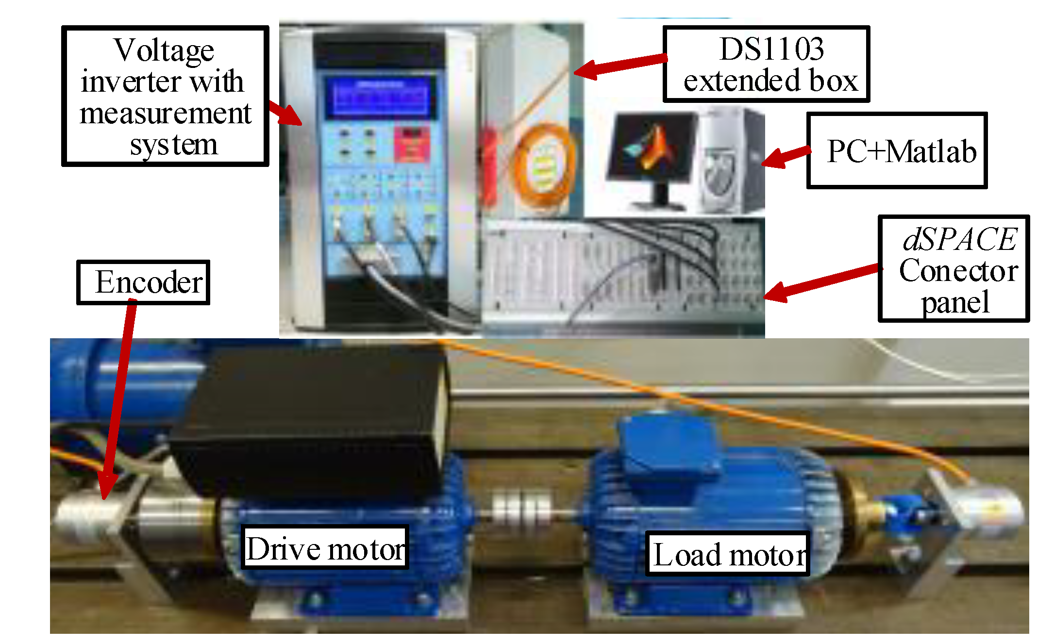
The following section is devoted to the presentation of the experimental results related to both control structures. Figure 2 depicts the block diagram of the experimental set-up, including an induction motor of nominal power 1.1 kW driven by a power converter. The motor and the load machine were connected with a shaft. Incremental encoders of 36,000 pulses provided measurement of the speed and position of the drive. A digital signal processor using the dSPACE 1103 calculated the control algorithms. The sampling time of the predictive controller was set to 0.2 ms. A simulation current model was utilized to estimate the rotor flux [47].

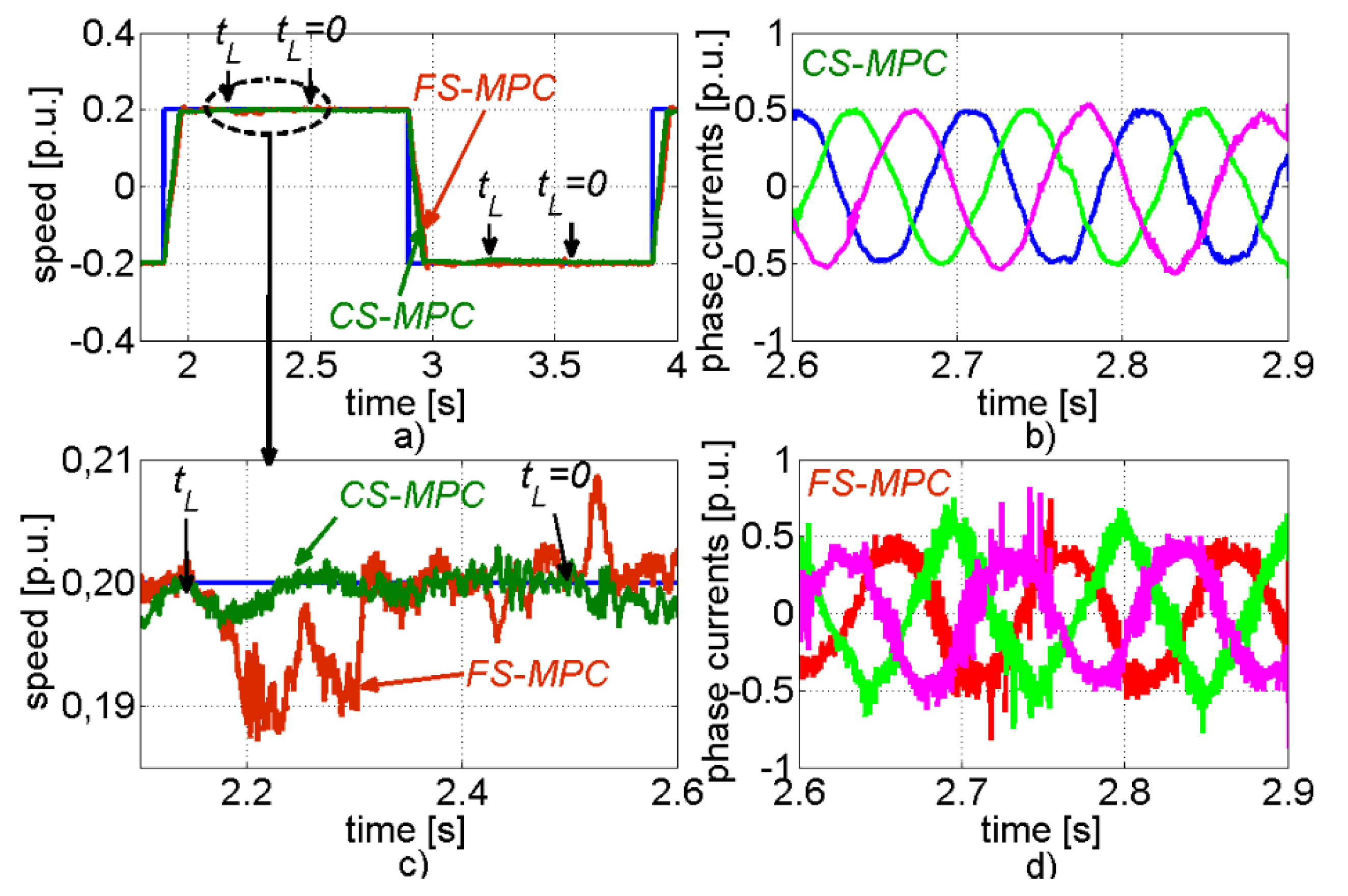
To begin with, both systems were tested under a reverse condition and for a low value of the reference speed. The drive worked under the following conditions. At time t = 1.9 s, the value of the reference signal changed from -0.2 to 0.2. The switching on and off of the load torque was performed at a time of 2.2 s and 2.5 s, respectively (it is marked in picture with arrow and description). At a time of 2.9 s the reference signal of the speed changed to -0.02. Then, the process of loading of the system was repeated. At a time of 2.9 s the negative set value was reversed. Some transients of the systems are shown in Figure 3.

In Figure 3 the transients of mechanical velocities (Figure 3a,c) and fragments of the currents (Figure 3b,d) are demonstrated in CS-MPC (a,b) and FS-MPC control structures. From the above-presented transients the following remarks can be formulated. Both control structures were working properly and followed the reference signal accurately. The raising time depended on the set driving torque limitation in the system. Applying the load torque resulted in the small disruption in the rotor speed, yet the CS-MPC structure possesses smaller speed fall. The difference between the two presented approaches is clearly visible in the shape of the stator currants (Figure 3b,d). In CS-MPC the currents contain much fewer high-frequency noises. It has an almost sinusoidal shape. Contrary to that, in FS-MPC the current possesses a lot of harmonics, stemming from the lack of a modulator in the system as well as the short prediction horizon.

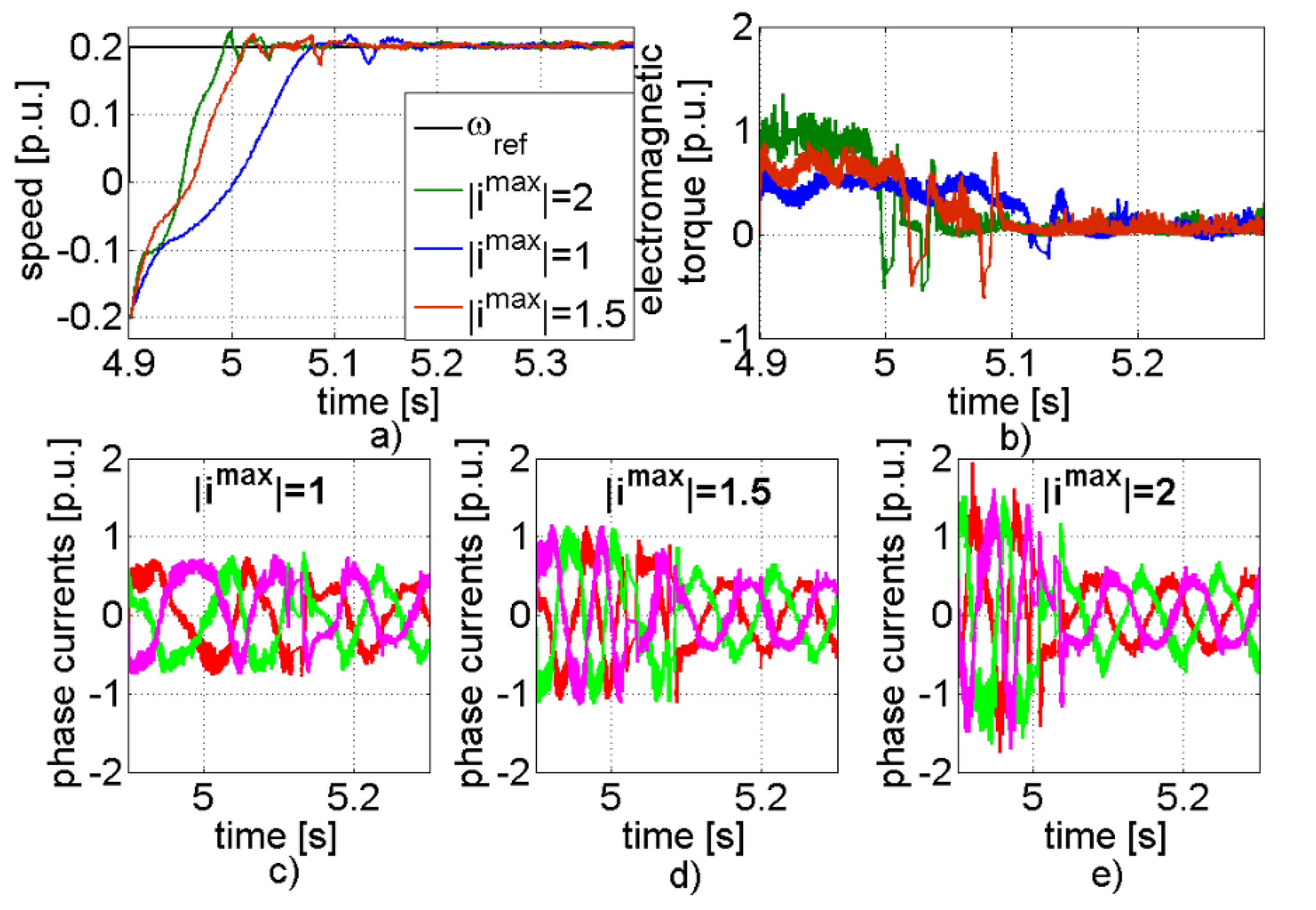
Next, the effect of the limitation of the stator current was investigated. The FS-MPC was analyzed first. In Figure 4 transients of the states are presented.

In Figure 4 transients of the speeds (a), driving torque (b), and stator current (c,d,e) for different values of the stator limitation (abs(i_max) = 1, 1.5 and 2) are presented. As can be concluded from Figure 4, the system worked correctly. Depending on the assumed signal limits, different torque levels and speed rising times were obtained. Despite correct work of the control structure, some oscillations were evident into torque transients. Those oscillations caused the shape of the speed transients during the raising time, which are not straight. The current possessed high frequency noises, which are characteristic for FS-MPC.

Then, the CS-MPC was investigated. Different values of the stator current component i_sy were set during tests. The obtained transients are presented in Figure 5.

The transients of the speeds, driving torque, and stator currents are presented in Figure 5 for CS-MPC for different values of the stator component limitation. In this case the electromagnetic torque transients had no oscillations. This resulted in the straight shape of the speed transients during start-up. Additionally, the overshoots in speed transients are much smaller than previously. The bigger the value of the limitation, the smaller the obtained settling time of the speed. The current transients were much smoother as compared to the FS-MPC. The set limitation value of the current was not violated.

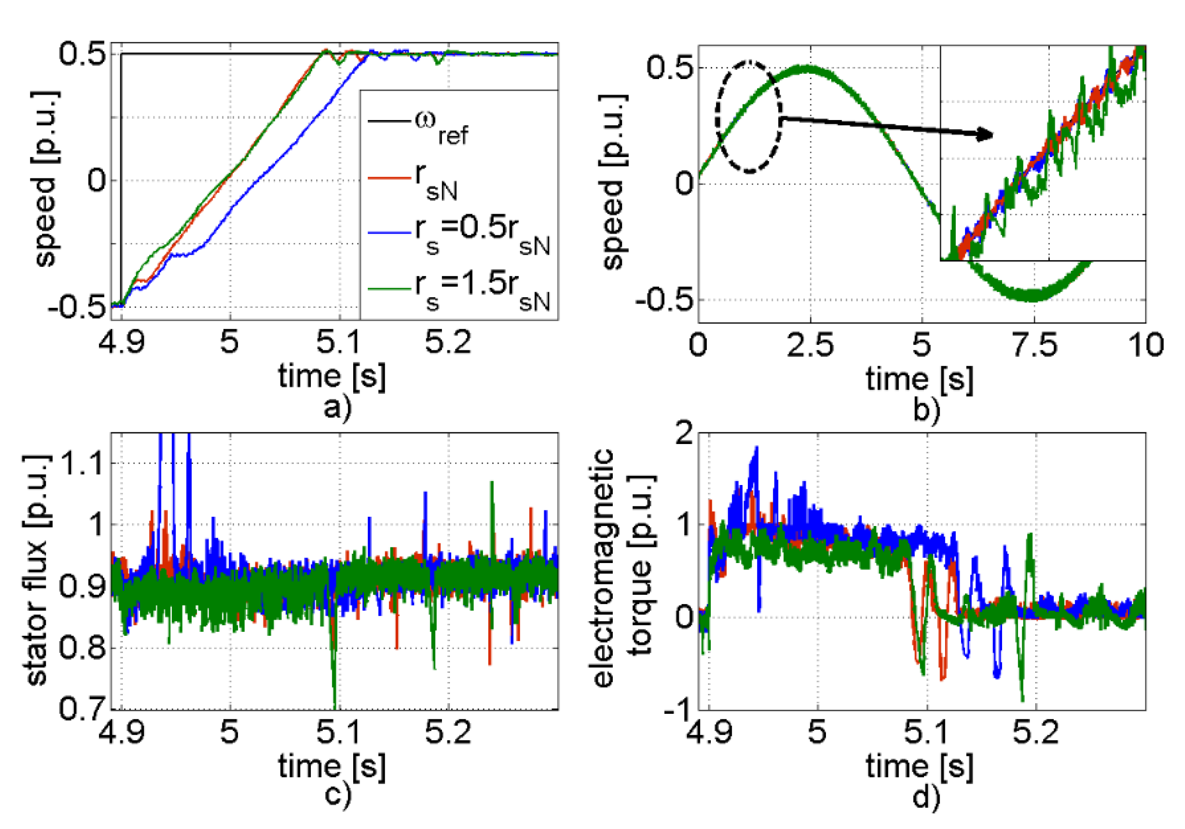
The robustness of both control algorithms for changes of the selected parameters of the IM was investigated. Firstly, the FC-MPC to the variation of the stator resistance and inertia of the rotor was tested. The value of the parameters was changed into the model of the object used in the algorithm. Some of the obtained transients are shown in Figure 6 and Figure 7.

In Figure 6, the speed, stator flux, and torque transients for different values of the stator resistance are presented. The reference value of the speed was set to the half of the nominal one. The system was working under reverse conditions. It should be noted that in this case the shape of the speed during start-up was straighter than for smaller value of the reference signal. The decrease of the value of the stator resistance influenced the system properties significantly. The settling time of the speed was bigger than for the other cases. Additionally, oscillations of the speed during transients were bigger (Figure 6b). The increase of the stator resistance value had a small effect on the system speed. The settling time of the speed was almost identical as for the nominal parameters. The stator flux was controlled correctly.

Then, the effect of the changing of the inertia was analyzed using transients presented in Figure 7. The following cases were considered: inertia equal to nominal value (J = J_n), decrease (J = 0.5J_n and J = 0.25J_n), and increase (J = 2J_n) of the inertia. The analyzed system worked under a reverse condition; the reference speed changed from 0.2 to −0.2. The transient of the speed, torque, and flux for the nominal system parameter is presented with the blue line. The increase of the inertia had a relatively small effect on the transients of the system. The shapes of the system variables were similar to the system with nominal parameters. Contrary to this, the decrease of the inertia can be seen more clearly in the transients. The settling time of the speed increased, and the hodograph of the flux was noisier.

Then, the performance of the CS-MPC was tested for the variation of the system parameters. The transients of the plant for changes of rotor resistance and inertia are shown in Figure 8 and Figure 9.

In Figure 8, transients of mechanical speeds (Figure 8a) and fragments of speeds (Figure 8b), rotor torques (Figure 8c), and electromagnetic torques (Figure 8d) are demonstrated for different values of the stator resistance. After analyzing the above-presented transients, the following conclusions can be reached. The changes of the stator resistance had a much smaller effect to the transients of the drive than in FS-MPC. The speed transients were similar. For the decreasing of the stator resistance the settling time of the speed was slightly bigger. The oscillation evident for speed transients was relatively small (Figure 8b). It resulted from the smooth shape of the torque transients (Figure 8d). Small fluctuations were evident in the rotor flux transients in all cases (Figure 8c).

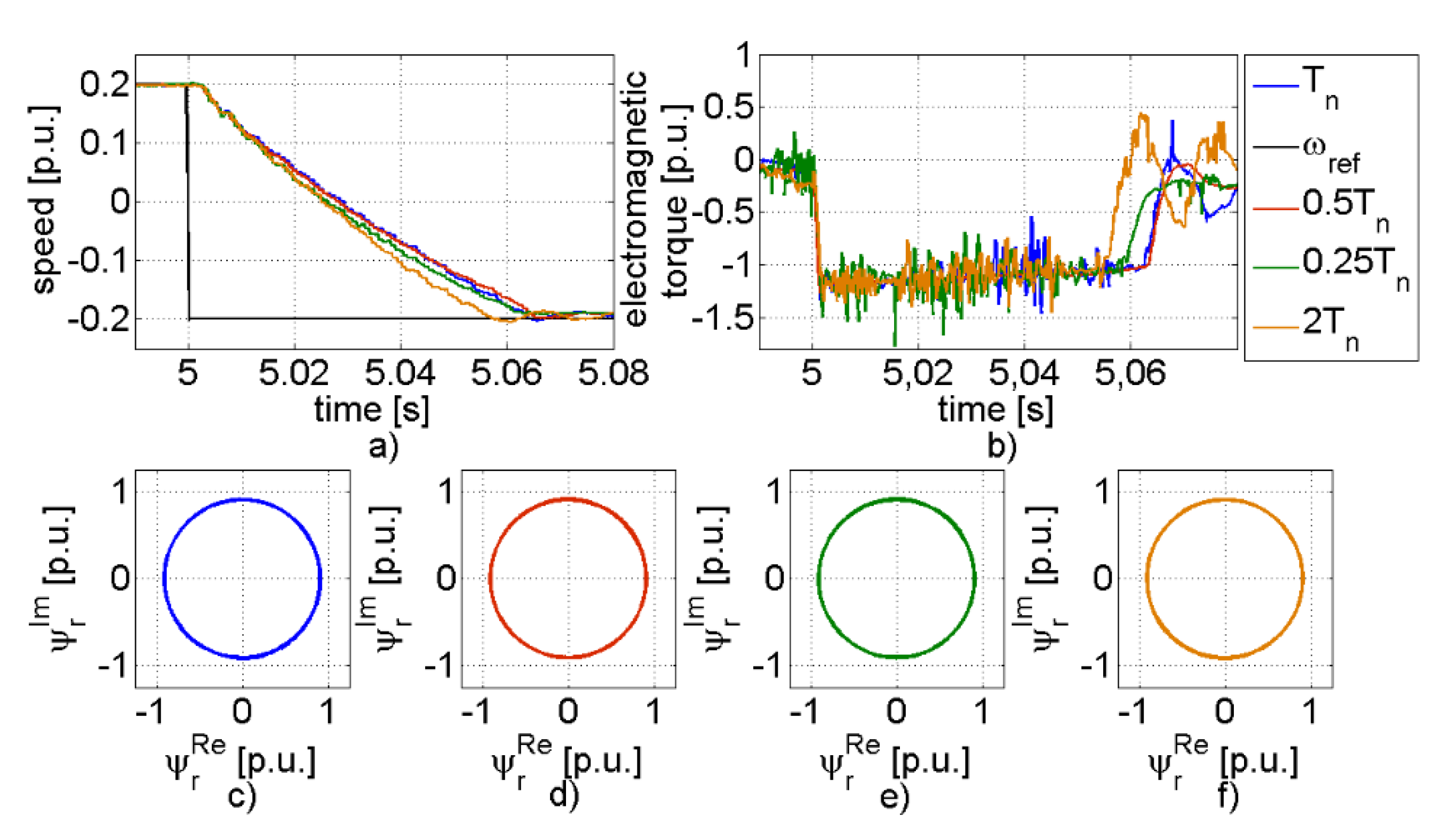
Then, the effect of the inertia changes on the properties of the system was investigated, similar to previous work, where the increase (J = 2J_n) and decrease (J = 0.5J_n and J = 0.25J_n) of inertia was considered. The transients of the speed (Figure 9a), torques (Figure 9b), and the rotor flux (Figure 9c) are presented. The quoted figures may lead to the following remarks. The changes of the inertia had limited impact on the transients of the drive in CS-MPC. The shape of all variables was similar for all cases. The differences between states were smaller than in the FC-MPC.

5. Conclusions

The core of this paper is a detailed investigation of two MPC-based control structures for speed control of an IM drive. The first control algorithm relies on FS-MPC approach, while the second one works with the use of the CS-MPC. Theoretical considerations and experimental validations may be summarized as follows.

When referring to the classical field-oriented control structure of the IM drive, the MPC approach seems to be an easier case at first glance. Instead of four classical PI controllers evident in the DFOC control structure, only one controller regulating all variables is visible.

Practical implementation of the long horizon CS-MPC is rather difficult due to the fact that this algorithm is computationally complex. Hence, the following steps should be taken. First, an IM model is made linear by means of inserting a decoupling circuit, i.e., the transformation blocks evident in DFOC, has to be applied. As a next step, the off-line MPC version is utilized in order to simplify the algorithm. This allows to decrease the complexity of traditional long-horizon MPC and run real time tests.

The mathematic model of IM does not include nonlinearities evident in the real system, such as the non-linear magnetizing characteristic, nonlinear friction. Those factors will reduce the performance in the drive especially in specific condition (e.g., in ultra- speed region). A similar problem arises for the change of the system parameters. Thus, the on-line version of MPC can be used, but the complexity of the algorithm increases as a result.

For the short horizon FS-MPC the optimization problem is solved on-line. Non-linearities may be included in the mathematical model of the plant in a natural way, which is why it is especially recommended for the low speed operation range. Moreover, when the parameters of the plant change, the changes can be easily incorporated in the algorithm.

In the control structure of CS-MPC the modulator is evident. It determines the constant value of the switching frequency. Contrary to this case, the modulator is not required in the FS-MPC. In this case the switching frequency is directly determinate as a function of the switches, which means that the modulation frequency is changeable. In order to hold it constant, the additional algorithm have to be applied.

In the FS-MPC, the phase currents possess many more components with high frequency. Those noises generate oscillations into electromagnetic torque. On the contrary, the CS-MPC results in the sinusoidal currents and smooth driving torque.

Both control algorithms allow for directly including the limitation (the control signal, state variables).

The proposed algorithms worked correctly in experimental tests. The reference signal as followed quickly by the system and changes of the load torque were removed swiftly. The constraints formulated in the control problem were not violated during the tests.

The CS-MPC is less sensitive to parameter changes of the plant, which results from the length of the horizon. In the CS-MPC it has a value of 10 samples, contrary to this approach, in FS-MPC only one sample is calculated ahead.

The attempt to increase the length of horizon in FS-MPC has been done. However, real-time implementation was not possible due to the computational requirements of the experimental processor. Thus, both implemented structures CS- and FS- need similar computational power.

References

- Grčar, B.; Hofer, A.; Štumberger, G. Induction Machine Control for a Wide Range of Drive Requirements. Energies 2020, 13, 175. [Google Scholar] [CrossRef] [Green Version]
- Benbouzid, M.E. A review of induction motors signature analysis as a medium for faults detection. IEEE Trans. Ind. Electron. 2000, 47, 984–993. [Google Scholar] [CrossRef] [Green Version]
- Tang, J.; Yang, Y.; Chen, J.; Qiu, R.; Liu, Z. Characteristics Analysis and Measurement of Inverter-Fed Induction Motors for Stator and Rotor Fault Detection. Energies 2020, 13, 101. [Google Scholar] [CrossRef] [Green Version]
- Hakami, S.; Saleh, M.; Alsofyani, I.; Lee, K. Low-Speed Performance Improvement of Direct Torque Control for Induction Motor Drives Fed by Three-Level NPC Inverter. Electronics 2020, 9, 77. [Google Scholar] [CrossRef] [Green Version]
- Li, Z.; Guo, Y.; Xia, J.; Li, H.; Zhang, X. Variable Sampling Frequency Model Predictive Torque Control for VSI-Fed IM Drives Without Current Sensors. IEEE J. Emerg. Sel. Top. Power Electron. 2020, 1, 1–11. [Google Scholar] [CrossRef]
- Blaschke, F. Das Verfahren der Feldorientierung zur Regelung der Asynchronmaschine. In Siemens Forschungs- und Entwicklungsberichte; Siemens AG: Berlin, Germany, 1972; pp. 184–193. [Google Scholar]
- Singh, V.K.; Tripathi, R.N.; Hanamoto, T. FPGA-Based Implementation of Finite Set-MPC for a VSI System Using XSG-Based Modeling. Energies 2020, 13, 260. [Google Scholar] [CrossRef] [Green Version]
- Wang, W.; Lu, Z.; Hua, W.; Wang, Z.; Cheng, M. Simplified Model Predictive Current Control of Primary Permanent-Magnet Linear Motor Traction Systems for Subway Applications. Energies 2019, 12, 4144. [Google Scholar] [CrossRef] [Green Version]
- Vazquez, S.; Rodriguez, J.; Rivera, M.; Franquelo, L.G.; Norambuena, M. Model Predictive Control for Power Converters and Drives: Advances and Trends. IEEE Trans. Ind. Electron. 2017, 64, 935–947. [Google Scholar] [CrossRef] [Green Version]
- Wang, F.; Mei, X.; Rodriguez, J.; Kennel, R. Model Predictive Control for Electrical Drive Systems—An Overview. CES Trans. Electr. Mach. Syst. 2019, 1, 219–230. [Google Scholar]
- Tenconi, A.; Rubino, S.; Bojoi, R. Model Predictive Control for Multiphase Motor Drives—A Technology Status Review. In Proceedings of the 2018 International Power Electronics Conference (IPEC-Niigata 2018 -ECCE Asia), Niigata, Japan, 20–24 May 2018; pp. 732–739. [Google Scholar]
- Vazquez, S.; Leon, J.I.; Franquelo, L.G.; Rodriguez, J.; Young, H.A.; Marquez, A.; Zanchetta, P. Model predictive control: A review of its applications in power electronics. IEEE Ind. Electr. Mag. 2014, 8, 16–31. [Google Scholar] [CrossRef]
- Gutierrez, B.; Kwak, S. Modular Multilevel Converters (MMCs) Controlled by Model Predictive Control with Reduced Calculation Burden. IEEE Trans. Power Electron. 2018, 33, 9176–9187. [Google Scholar] [CrossRef]
- Karamanakos, P.; Geyer, T.; Aguilera, R.P. Computationally Efficient Long-Horizon Direct Model Predictive Control for Transient Operation. In Proceedings of the 2017 IEEE Energy Conversion Congress and Exposition (ECCE), Cincinnati, OH, USA, 1–5 October 2017; pp. 4642–4649. [Google Scholar]
- Karamanakos, P.; Geyer, T.; Aguilera, R.P. Long-Horizon Direct Model Predictive Control: Modified Sphere Decoding for Transient Operation. IEEE Trans. Ind. Appl. 2018, 54, 6060–6070. [Google Scholar] [CrossRef]
- Fehér, M.; Straka, O.; Šmídl, V. Model predictive control of electric drive system with L1-norm. Eur. J. Control 2020, 1–12. [Google Scholar] [CrossRef]
- Wang, L.; Tan, G.; Meng, J. Research on Model Predictive Control of IPMSM Based on Adaline Neural Network Parameter Identification. Energies 2019, 12, 4803. [Google Scholar] [CrossRef] [Green Version]
- Gonçalves, P.; Cruz, S.; Mendes, A. Finite Control Set Model Predictive Control of Six-Phase Asymmetrical Machines—An Overview. Energies 2019, 12, 4693. [Google Scholar] [CrossRef] [Green Version]
- Kuoro, S.; Perez, M.A.; Rodriguez, J.; Llor, A.M.; Young, H.A. Model Predictive Control: MPC’s Role in the Evolution of Power Electronics. IEEE Ind. Electr. Mag. 2015, 9, 8–21. [Google Scholar] [CrossRef]
- Gonzales, O.; Ayala, M.; Doval-Gandoy, J.; Rodas, J.; Gregor, R.; Rivera, M. Predictive-Fixed Switching Current Control Strategy Applied to Six-Phase Induction Machine. Energies 2019, 12, 2294. [Google Scholar] [CrossRef] [Green Version]
- Aciego, J.J.; González Prieto, I.; Duran, M.J. Model Predictive Control of Six-Phase Induction Motor Drives Using Two Virtual Voltage Vectors. IEEE J. Emerg. Sel. Top. Power Electron. 2019, 7, 321–330. [Google Scholar] [CrossRef]
- Agustin, C.; Almazan, Y.J.; Lin, C.; Fu, X. A Modulated Model Predictive Current Controller for Interior Permanent-Magnet Synchronous Motors. Energies 2019, 12, 2885. [Google Scholar] [CrossRef] [Green Version]
- Dorfling, T.; Mouton, H.D.; Geyer, T.; Karamanakos, P. Long-Horizon Finite-Control-Set Model Predictive Control with Non-Recursive Sphere Decoding on an FPGA. IEEE Trans. Power Electron. 2019, 1, 1–12. [Google Scholar] [CrossRef]
- Liu, F.; Kang, E.; Cui, N. Single-loop model prediction control of PMSM with moment of inertia identification. IEEJ Trans. Electr. Electron. Eng. 2020, 15, 1–7. [Google Scholar] [CrossRef]
- Wang, Y.; Li, H.; Liu, R.; Yang, L.; Wang, X. Modulated Model-Free Predictive Control With Minimum Switching Losses for PMSM Drive System. IEEE Access 2020, 8, 20942–20953. [Google Scholar] [CrossRef]
- Petkar, S.G.; Eshwar, K.; Thippiripati, V.K. A Modified Model Predictive Current Control of Permanent Magnet Synchronous Motor Drive. IEEE Trans. Ind. Electron. 2020, 1, 1–9. [Google Scholar] [CrossRef]
- Alsofyani, I.; Mohd, L.K. Improved Deadbeat FC-MPC Based on the Discrete Space Vector Modulation Method with Efficient Computation for a Grid-Connected Three-Level Inverter System. Energies 2019, 12, 3111. [Google Scholar] [CrossRef] [Green Version]
- Andersson, A.; Thiringer, T. Assessment of an Improved Finite Control Set Model Predictive Current Controller for Automotive Propulsion Applications. IEEE Trans. Ind. Electron. 2020, 67, 91–100. [Google Scholar] [CrossRef]
- Arahal, M.R.; Martin, C.; Kowal, A.; Castilla, M.; Barrero, F. Cost function optimization for predictive control of a five-phase IM drive. Optim. Control. Appl. Methods 2020, 41, 84–93. [Google Scholar] [CrossRef] [Green Version]
- Wendel, S.; Haucke-Korber, B.; Dietz, A.; Kennel, R. Experimental Evaluation of Cascaded Continuous and Finite Set Model Predictive Speed Control for Electrical Drives. In Proceedings of the 2019 21st European Conference on Power Electronics and Applications (EPE’ 19 ECCE Europe), Genova, Italy, 2–5 September 2019; pp. 1–10. [Google Scholar]
- Garayalde, E.; Aizpuru, I.; Iraola, U.; Sanz, I.; Bernal, C.; Oyarbide, E. Finite Control Set MPC vs Continuous Control Set MPC Performance Comparison for Synchronous Buck Converter Control in Energy Storage Application. In Proceedings of the 2019 International Conference on Clean Electrical Power (ICCEP), Otranto, Italy, 2–4 July 2019; pp. 490–495. [Google Scholar]
- Ileš, Š.; Bariša, T.; Sumina, D.; Matuško, J. Hybrid CCS/FCS Model Predictive Current Control of a Grid Connected Two-Level Converter. In Proceedings of the 2018 IEEE 18th International Power Electronics and Motion Control Conference (PEMC), Budapest, Hungary, 26–30 August 2018; pp. 981–986. [Google Scholar]
- Jun, E.; Park, S.; Kwak, S. A Comprehensive Double-Vector Approach to Alleviate Common-Mode Voltage in Three-Phase Voltage-Source Inverters with a Predictive Control Algorithm. Electronics 2019, 8, 872. [Google Scholar] [CrossRef] [Green Version]
- Jun, E.; Park, S.; Kwak, S. Model Predictive Current Control Method with Improved Performances for Three-Phase Voltage Source Inverters. Electronics 2019, 8, 625. [Google Scholar] [CrossRef] [Green Version]
- Townsend, C.D.; Mirzaeva, G.; Goodwin, G.C. Short-Horizon Model Predictive Modulation of Three-Phase Voltage Source Inverters. IEEE Trans. Ind. Electron. 2018, 65, 2945–2955. [Google Scholar] [CrossRef]
- Bao, G.; Qi, W.; He, T. Direct Torque Control of PMSM with Modified Finite Set Model Predictive Control. Energies 2020, 13, 234. [Google Scholar] [CrossRef] [Green Version]
- Wang, F.; Zhang, Z.; Mei, X.; Rodriguez, J.; Kennel, R. Advanced Control Strategies of Induction Machine: Field Oriented Control, Direct Torque Control and Model Predictive Control. Energies 2018, 11, 120. [Google Scholar] [CrossRef] [Green Version]
- Feng, S.; Wei, C.; Lei, J. Reduction of Prediction Errors for the Matrix Converter with an Improved Model Predictive Control. Energies 2019, 12, 3029. [Google Scholar] [CrossRef] [Green Version]
- Lei, T.; Tan, W.; Chen, G.; Kong, D. A Novel Robust Model Predictive Controller for Aerospace Three-Phase PWM Rectifiers. Energies 2018, 11, 2490. [Google Scholar] [CrossRef] [Green Version]
- Ahmed, A.A.; Koh, B.K.; Lee, Y.I. A Comparison of Finite Control Set and Continuous Control Set Model Predictive Control Schemes for Speed Control of Induction Motors. IEEE Trans. Ind. Inform. 2018, 14, 1334–1346. [Google Scholar] [CrossRef]
- Preindl, M.; Bolognani, S. Comparison of Direct and PWM Model Predictive Control for Power Electronic and Drive Systems. In Proceedings of the 2013 Twenty-Eighth Annual IEEE Applied Power Electronics Conference and Exposition (APEC), Long Beach, CA, USA, 17–21 March 2013; pp. 2526–2533. [Google Scholar]
- Koiwa, K.; Kuribayashi, T.; Zanma, T.; Liu, K.; Wakaiki, M. Optimal current control for PMSM considering inverter output voltage limit: Model predictive control and pulse-width modulation. IET Electr. Power Appl. 2019, 13, 2044–2051. [Google Scholar] [CrossRef]
- Wang, L. Model Predictive Control System Design and Implementation Using MATLAB, Advances in Industrial Control; Springer Science & Business Media: London, UK, 2009. [Google Scholar]
- Chai, S.; Wang, L.; Rogers, E. Model predictive control of a permanent magnet synchronous motorwith experimental validation. Control Eng. Pract. 2013, 21, 1584–1593. [Google Scholar] [CrossRef]
- Kvasnica, M.; Grieder, P.; Baotić, M.; Morari, M. Multi-Parametric Toolbox (MPT). Hybrid Systems: Computation and Control, HSCC 2004. Lect. Notes Comput. Sci. 2004, 2993, 448–462. [Google Scholar]
- Herceg, M.; Kvasnica, M.; Jones, C.N.; Morari, M. Multi-Parametric Toolbox 30. In Proceedings of the 2013 European Control Conference (ECC), Zurich, Switzerland, 17–19 July 2013; pp. 502–510. [Google Scholar]
- Orłowska-Kowalska, T. Speed Sensorless Induction Motor Drives; Wrocław University of Technology Press: Wroclaw, Poland, 2003. (In Polish) [Google Scholar]
Figure 1.
The CS-MPC (a) and FS-MPC (b) based control structure.
Figure 2.
The block diagram of the laboratory set-up.
Figure 3.
Selected transients of the CS-MPC (a,b) and FC-MPC (c,d) structures: speed transients (a,c) and fragment of the stator currents (b,d) for the value of the reference signal equal ωref = 0.2.
Figure 4.
Selected transients of the FS-MPC: speed (a), electromagnetic torque (b), and currents (c,d,e) for different value of the stator current limitation: abs(imax) = 1, 1.5, and 2 and ωref = 0.2.
Figure 5.
Selected transients of the CS-MPC: speed (a), driving torque (b), and currents (c,d,e) for different value of the stator current limitation: isy = 1, 1.5, and 2 and value of the reference signal ωref = 0.2.
Figure 6.
Selected transients of the FS-MPC: speeds (a), fragment of speeds (b), stator flux (c), and driving torques (d) for various value of the stator resistance and value of the reference signal ωref = 0.5.
Figure 7.
Selected transients of the FS-MPC: speeds (a), electromagnetic torques (b), and stator flux for various value of the motor inertia: Jn (c); 0.5Jn (d); 0.25Jn (e); 2Jn (f).
Figure 8.
Selected transients of the CS-MPC: speeds (a), fragment of speeds (b), stator flux (c), and driving torques (d) for different values of the stator resistance and of the reference signal value ωref = 0.5.
Figure 9.
Selected transients of the CS-MPC: speeds (a), electromagnetic torques (b), and stator flux for different values of the motor inertia: Tn (c); 0.5Tn (d); 0.25Tn (e); 2Tn (f).
© 2020 by the authors. Licensee MDPI, Basel, Switzerland. This article is an open access article distributed under the terms and conditions of the Creative Commons Attribution (CC BY) license (http://creativecommons.org/licenses/by/4.0/).
Share and Cite
MDPI and ACS Style
Wróbel, K.; Serkies, P.; Szabat, K. Model Predictive Base Direct Speed Control of Induction Motor Drive—Continuous and Finite Set Approaches. Energies 2020, 13, 1193. https://doi.org/10.3390/en13051193
AMA Style
Wróbel K, Serkies P, Szabat K. Model Predictive Base Direct Speed Control of Induction Motor Drive—Continuous and Finite Set Approaches. Energies. 2020; 13(5):1193. https://doi.org/10.3390/en13051193
Chicago/Turabian StyleWróbel, Karol, Piotr Serkies, and Krzysztof Szabat. 2020. "Model Predictive Base Direct Speed Control of Induction Motor Drive—Continuous and Finite Set Approaches" Energies 13, no. 5: 1193. https://doi.org/10.3390/en13051193
Note that from the first issue of 2016, this journal uses article numbers instead of page numbers. See further details here.