A Novel Accurate and Fast Converging Deep Learning-Based Model for Electrical Energy Consumption Forecasting in a Smart Grid ^†

Abstract

Energy consumption forecasting is of prime importance for the restructured environment of energy management in the electricity market. Accurate energy consumption forecasting is essential for efficient energy management in the smart grid (SG); however, the energy consumption pattern is non-linear with a high level of uncertainty and volatility. Forecasting such complex patterns requires accurate and fast forecasting models. In this paper, a novel hybrid electrical energy consumption forecasting model is proposed based on a deep learning model known as factored conditional restricted Boltzmann machine (FCRBM). The deep learning-based FCRBM model uses a rectified linear unit (ReLU) activation function and a multivariate autoregressive technique for the network training. The proposed model predicts future electrical energy consumption for efficient energy management in the SG. The proposed model is a novel hybrid model comprising four modules: (i) data processing and features selection module, (ii) deep learning-based FCRBM forecasting module, (iii) genetic wind driven optimization (GWDO) algorithm-based optimization module, and (iv) utilization module. The proposed hybrid model, called FS-FCRBM-GWDO, is tested and evaluated on real power grid data of USA in terms of four performance metrics: mean absolute percentage deviation (MAPD), variance, correlation coefficient, and convergence rate. Simulation results validate that the proposed hybrid FS-FCRBM-GWDO model has superior performance than existing models such as accurate fast converging short-term load forecasting (AFC-STLF) model, mutual information-modified enhanced differential evolution algorithm-artificial neural network (MI-mEDE-ANN)-based model, features selection-ANN (FS-ANN)-based model, and Bi-level model, in terms of forecast accuracy and convergence rate.

1. Introduction

Electrical energy consumption forecasting is imperative for efficient energy management in the supply and demand sector of the smart grid (SG) [1]. It is significant in the supply side due to two reasons: (i) lack of viable planning of resources to efficiently cope with the consumers’ demand, and (ii) energy is an irreversible process and cannot be stored. Precise and accurate electric load forecast facilitates efficient load dispatch in power utilities and transaction markets. On the other hand, it is indefensible in the demand side, because electric load forecasting optimizes the energy management system and equipment use. Moreover, it also plays an imperative role in ensuring secure operations of the SG [2]. Energy theft is one of the major threats faced by the SG. It takes place when an adversary compromises the smart meters to send tampered consumption readings, which could lead to economic losses. Electrical energy consumption forecasting can be used in identifying possibly compromised smart meters whose behaviors significantly deviate from the forecasted ones. However, the accuracy of electrical energy consumption forecasting cannot often cope with the societal requirements. It is influenced by stochastic and uncertain influencing factors, such as human social activities, temperature, irradiance weather parameters, environmental parameters, economic development, climate change, and state policies. Consequently, it is challenging to improve the accuracy of forecasting networks. It is unrealistic or cumbersome to consider all the influencing factors [3]. Thus, it is feasible to improve the forecast accuracy by developing a model that takes into account the key parameters.

Over the past few decades, numerous methods have been developed and employed for accurate electrical energy consumption forecasting, such as obsolete time series models including Kalman filters [4], exponential smoothing [5], grey forecasting model (GM) [6], regression models [7,8], and autoregressive integrated moving average (ARIMA) models [9]. The existing forecasting models are capable of forecasting electrical energy consumption patterns. However, the accuracy is not good enough due to the networks’ inherent limitations. The linear regressors are knowledge-based and are suitable for linear problems, while their performance would compromise when solving non-linear problems. The ARIMA models consider current and historical data points to forecast and ignore other influencing factors. The GM model is suitable to handle only exponential growth trend problems. To overcome the limitations accompanied by the discussed models, in recent years, intelligent models have been proposed for forecasting such as artificial neural network (ANN) [10,11], machine learning [12], radial basis fuzzy logic [13], and expert systems [14]. Though intelligent methods outperform classical statistical methods, ANN based models stuck in local minima, radial basis logic methods are radially invertible, and expert systems need knowledge databases. Thus, hybrid forecasting models are developed, where individual modules are integrated. For instance, in [15], authors proposed an integrated framework of support vector machine (SVM) and modified enhanced differential evaluation (mEDE) algorithm. The authors in [16] developed a hybrid model using support vector regression (SVR) and chaotic particle swarm optimization (CPSO) algorithm. In [17], the authors designed a hybrid model of SVM and artificial intelligence (AI) for load forecasting. The hybrid and integrated models are superior than single and individual module-based models in terms of forecast accuracy.

As discussed, ANN-based models are widely used for forecasting; however, these models are trapped into local minima due to the restriction on their generalization ability and therefore, cannot select abstracted features from the given sample set. A deep learning model, known as factored conditional restricted Boltzmann machine (FCRBM), overcomes these drawbacks and reduces the error metric to improve the forecast accuracy. FCRBM employs learning principles with ReLU to increase generalization in the training process and generate accurate forecasts. Because of the deeper layer layout, attractive features, and empirical performance, FCRBM has become one of the most popular and promising forecasting models [18]. Therefore, in this paper, a deep learning FCRBM is used in the forecaster module for forecasting. The irrelevant and redundant information directly affects accuracy and convergence rate. Therefore, a novel concept of the candidates’ interaction is introduced in addition to the redundancy and relevancy filters. The proposed genetic wind driven optimization (GWDO) algorithm [19,20] is chosen, among other algorithms, due to its fast convergence and powerful ability to search an optimal solution [21]. GWDO optimizes the thresholds of these filters and feeds the optimized thresholds to the feature selection module for feature selection. This, in turn, improves the accuracy.

In this article, a novel hybrid model is proposed, which is an integrated framework of data processing and feature selection technique, a deep learning FCRBM model, and our proposed GWDO algorithm (FS-FCRBM-GWDO). The performance of the proposed FS-FCRBM-GWDO model is validated by comparing it with existing models in terms of three performance metrics: mean absolute percentage deviation (MAPD), variance, and correlation. The major contributions are described as follows:

• A novel hybrid FS-FCRBM-GWDO forecast model is proposed that integrates the merits of individual techniques to enhance both metrics: (i) accuracy (MAPD, variance, and correlation), and (ii) convergence rate. The proposed model is capable of mapping the input space to the feature space to learn the stochastic and complex patterns of electrical energy consumption.
• The proposed FS-FCRBM-GWDO model considers both the exogenous influencing parameters and the historical electrical energy consumption pattern.
• A novel concept of feature interaction is developed in addition to relevancy and redundancy filters of feature selection techniques to make the feature selection process more effective.
• The ReLU and multivariate autoregressive algorithms are integrated with FCRBM to improve both accuracy and convergence rate, which are not present in the existing models.
• The GWDO algorithm is proposed for the optimization module to further reduce error in the forecasting results returned from the FCRBM based forecaster by fine-tuning the control parameters.

The remainder of the manuscript is organized as follows: The recent and relevant work is demonstrated in Section 2. In Section 3, the proposed hybrid FS-FCRBM-GWDO model is described. The results of our simulations are presented and discussed in Section 4. Finally, in Section 5, the manuscript is concluded with potential future directions. Abbreviations and notations used in this work are listed at the end of the paper.

2. Related Work

Electrical energy consumption forecasting strategies have been proposed for the past many years and employed in the SG for efficient energy management. These strategies are categorized into four classes according to time resolution [22]. The first class is about very short-term energy consumption forecasting [23], which corresponds to the energy consumption forecasting of time resolution from minutes to hours. The second class is about short-term electrical energy consumption forecasting of time resolution from days to a week [24]. The third class is the medium-term electrical energy consumption forecasting of time resolution from one week to a year [25]. The fourth class is about the long-term electrical energy consumption forecasting of time resolution for more than a year [26].

Classical statistical methods and intelligent methods are commonly used for electrical energy consumption forecasting. ANN is widely used as an intrinsic system and as a part of the hybrid system for electric load forecasting. In [27], Kohonen’s self-organizing map is used for the day ahead electric load forecasting in Spain. The described strategy comprises three stages. The daily load profile is treated as a time series and is stored in the neurons; After the training phase, the arrangement of neurons is such that the load profile given to the neuron is similar to the neighboring neurons. During the second phase, the data samples are presented to the network and wining neurons are extracted. Then, the data samples of the winning neurons are divided into two parts. The first one corresponds to the input profile and the second one corresponds to the forecasted profile. The effect of exogenous parameters on accuracy is also considered. It is also reported that the percentage error varied from 1.84% to 2.33%. A differential polynomial neural network for short-term load forecasting is described in [28]. The network is a multi-layer network and by its decomposition, partial differential equations are solved. The twenty-four hours ahead load is forecasted using the historical electric load data of Canada. The forecasted energy consumption pattern deviates from the target pattern by an error of 1.56%. A short-term load forecasting method based on weather information is proposed in [29]. The power system is divided into subnetworks based on weather information. Separate models are developed for each subnetwork. The abstracted features are selected form large data sets using cosine distance method. The models are based on ANN, ARIMA, and GM to forecast the future load. A hybrid forecast strategy is proposed in [30] based on an intelligent algorithm. The strategy includes a novel feature selection technique and a complex forecast engine. A novel features selection technique selects appropriate features that are fed into the forecast engine. The forecast engine is two-staged and is implemented on Reglet and Elman neural network. The intelligent algorithm tunes the adjustable parameters of the forecast engine for improving accuracy along with a reasonable convergence rate. The performance of the described model is evaluated by comparing it with the benchmark models. A deep learning-based forecasting framework with appliances energy consumption sequence is proposed in [31]. The accuracy is notably improved by incorporating appliances consumption sequences in addition to the deep neural network. An integrated framework of the forecaster module based on deep learning and optimization module based on the heuristic algorithm is proposed for electric load forecasting [32].

The authors in [33], proposed an Elman neural network-based forecast engine to predict the future load in the SG. The weights and biases for this network are optimally adjusted by an intelligent algorithm to obtain accurate forecasting results. The authors proposed a novel forecasting model that could generalize the standard ARMAX model to Hilbert space [34]. The proposed model has a linear regression structure and uses functional variables for operation. The considered variables are autoregressive terms, moving average terms, and exogenous parameters. The functional variables are integral operators whose kernels are modeled as sigmoidal function. The parameters of the sigmoidal function are optimized using the quasi-newton algorithm. The model is validated on the daily price profile of the Spanish and German electricity market. However, accuracy is enhanced due to the optimization module integration, which increases the execution time. In [35], authors reveal the effect of data integrity attacks on the accuracy of four forecasting models: SVR, multiple linear regression, ANN, and fuzzy interaction regression. The data integrity attacks attempt to damage the performance of various forecasting models and have a significant impact on the resilience of the power system.

In the aforementioned recent and relevant work, authors mostly focused on ANN-based models for electrical energy consumption prediction due to its capability for handling the nonlinear electrical energy consumption pattern. However, the ANN-based forecasters perform well for small data but do not behave well for large data in terms of accuracy. In this regard, in the literature, either the optimization module is integrated with ANN-based forecaster or deep learning models are adopted to improve the forecast accuracy. However, the optimization module and deep learning models cause high execution time overhead while improving the accuracy. The recent and relevant research in terms of techniques, objectives, datasets, limitations, and critical remarks is summarized in

Table 1. Brief review of recent and relevant work in terms of techniques, objectives, datasets, limitations, and critical remarks.

Techniques	Objectives	Datasets	Limitations	Critical Remarks
ARIMA and exponential smoothing [23]	Forecast accuracy improvement for power generation scheduling in real-time.	National grid and Great Britain	This model is useful for only very short term load forecasting.	The prime focus of authors is on accuracy improvements for univariate methods while the accuracy improvement of univariate is not sufficient.
ANN and self-organizing map [27]	To build a decision support system for commercializing company bidding.	Spain power grid	This model achieves moderate accuracy at the cost of slow convergence rate (high execution time).	Meteorological and load data is used in this model and other exogenous parameters are ignored that significantly affect the forecast accuracy.
Differential polynomial neural network [28]	Reduction of generation cost and spinning reserve capacity.	Canada power grid	Unnecessary and overload prediction leads to large reserves and high cost.	Slow convergence and less accuracy is observed in this model, which have a direct impact on cost and spinning reserve.
ANN, ARIMA, and GM [29]	To improve the accuracy of bulk power system.	China Fujian Province power grid	The system becomes more complex by dividing the system into subnetworks.	Improvement in accuracy by using large exogenous parameters at the cost of high complexity and slow convergence rate.
Reglet and Elman neural network [30]	Accuracy and capability improvement for efficient operation of the power system.	Australian energy market commission	The model has large complexity.	This model has a large complexity that directly impacts the convergence rate.
Long term short term memory [31]	Forecast accuracy improvement for household scheduling.	Canadian household	The system model has slow convergence due to the incorporation of household appliances sequence.	The accuracy is notably improved using appliances consumption sequence, however, the convergence rate is compromised.
SVR [33]	Improvement of load forecasting accuracy for minimizing cost and energy imbalance.	Irish commission for energy regulation (ICER)	The model has a slow convergence speed.	The hyperparameters are tuned by the intelligent techniques which improved accuracy at the expense of increased execution time.
ARIMAX and quasi-newton algorithm [34]	Improvement of forecast accuracy for system operators and the market agent.	Spanish and German energy market	The convergence speed is compromised.	They improved accuracy is improved due to incorporating of sigmoid function. However, the computational time is increased.
ANN, SVR, and fuzzy interaction regression [35]	Improvement of resilience against attacks on data integrity.	Global energy forecasting competition (GEFC) 2012	The resilience is improved at increased time complexity.	The power system resiliency is enhanced at the expense of higher complexity of modeling.
MI, ANN, and mEDE [36,37]	Improvement of convergence rate and accuracy for US EKPC and Dayton grid.	PJM market	The complexity of the model is increased.	The developed model outperforms for small datasize and worst perform for large datasize.
ANN-based hybrid models [38,39]	Microgrid accuracy improvement.	PJM market	The convergence rate is compromised while improving forecast accuracy.	The ANN forecaster improved the accuracy, which degrade the execution time.

.

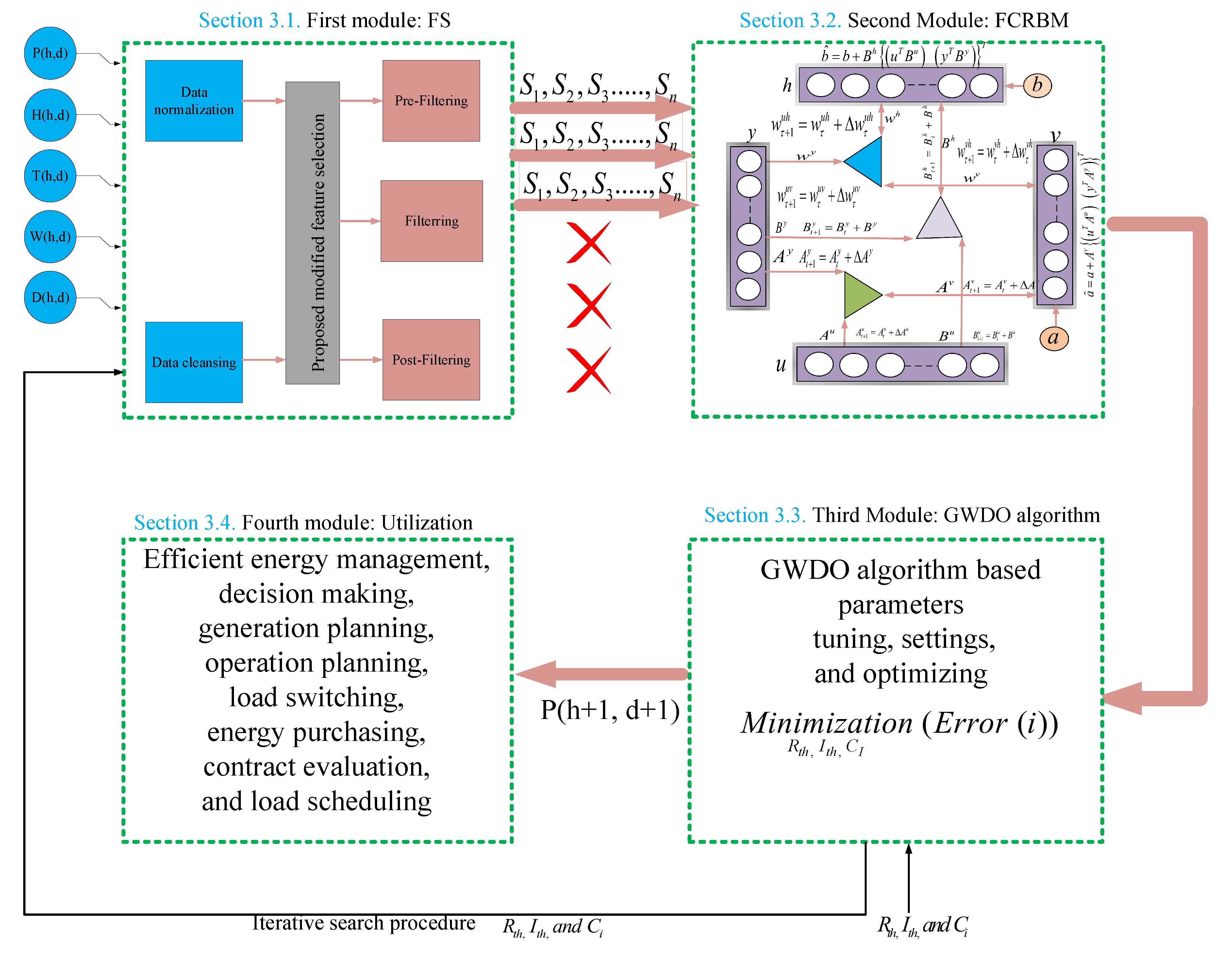
3. The Proposed Deep Learning-Based Hybrid Model

A novel hybrid FS-FCRBM-GWDO model for electrical energy consumption forecasting is proposed, as illustrated in Figure 1, which is an extension of our earlier conference paper [40]. The proposed hybrid model aims to improve forecast accuracy, convergence speed, and scalability. FS-FCRBM-GWDO is composed of four modules: (i) data processing and feature selection module, (ii) FCRBM-based forecasting module, (iii) GWDO-based optimization module, and (iv) utilization module. Both historical energy consumption pattern data and exogenous parameters (wind speed, dew point, temperature, and humidity) are given as input to the data processing and features selection module. At first, the received input data is normalized and passed through the relevancy, redundancy, and interaction phases. This module aims to clean the data and select abstractive features for the forecast process by maximizing relevancy, minimizing redundancy, and maximizing features interaction. The selected features are fed into the FCRBM-based forecasting module. The purpose is to predict the future electrical energy consumption pattern of the FE power grid. The forecasted energy consumption is fed into the optimization module based on the GWDO algorithm. The objective is to enhance forecast accuracy, which is very important for efficient energy management. Finally, the forecasted energy consumption pattern is fed into the utilization module to use the predicted energy consumption pattern for efficient energy management in the SG. The detailed demonstration is as follows:

3.1. Data Processing and Features Selection Module

The input dataset that has both historical energy consumption pattern and exogenous parameters (wind speed, dew point, temperature, and humidity) is fed for pre-processing and feature selection. First, the dataset is passed through the cleansing phase to recover missing and not a number (NAN) values with average or median values of the previous day. Then, the cleansed data is fed to the normalization operation using Equation (1) to make data entries within the limit of the activation function:

$$Norm=\frac{X-\mu (X)}{std(X),}$$

(1)

where Norm is the normalized data, X is the input data, and std is the standard deviation. The input data (X) includes electrical energy consumption data pattern ($P(h,d)$), dew point ($D(h,d)$), temperature ($T(h,d)$), and humidity $(H(h,d))$ parameters. The hour h and day d represents particular hour and day, respectively, in historical data. The wind speed, dew point, temperature, and humidity are called exogenous parameters. Energy demand shows the correlation with variation in exogenous parameters. For example, increase or decrease in the external temperature induces changes in energy demand. Same applies to the other parameters. The FS technique has irrelevancy, redundancy filters, and features interaction phase in order to remove irrelevant, redundant, and nonconstructive information due to three reasons: (i) redundant information is not useful and causes execution overhead during the training phase, (ii) irrelevant features do not provide useful information and act as an outlier, and (iii) interacting features provide useful information to enhance electrical energy consumption forecast accuracy. The relevancy, redundancy filters, and feature interaction phases are discussed as follows:

3.1.1. Relevancy Filter Operation

For feature selection relevancy operation is of great importance because input features and target variables are correlated in order to select key features. Many techniques for relevancy measurement are used [41] among feature selection techniques. The chosen FS technique measures mutual information to ensure how closely the two variables x and y are correlated. The FS technique observes y by studying x and vice versa. For variables x and y, the FS is represented by $I(x;y)$ and is defined for individual ($p(x),p(y)$) probability distribution as well as for joint probability distribution ($p(x,y)$). Suppose that

$$S=\{x_1,x_2,x_3,\dots ,x_M\},$$

(2)

where $x_1,x_2,x_3,\dots ,x_M$ are input variables, S is input variables set and the target variable is y. The mutual information between input $x_i$ and target y variables are checked; when the mutual information between two variables is large enough, they are closely related. In addition, the relevance of input $x_i$ variable with target y variable is computed as follows:

$$D(x_i)=I(x_i;y),$$

(3)

where $D(x_i)$ denotes the relevance of the input variable with the target variable.

3.1.2. Redundancy Filter Operation

Several authors in [42,43,44] developed redundancy filter operation to check the redundancy among input variables because redundant information complicates the process and increases the convergence speed. The redundancy evaluation is performed among the input candidates based on mutual information. The purpose is to discard redundant features. The authors in [41] stated that closely related input variables degrade the feature selection process. This is because two input variables have more common information and very little redundant information about the target variable. Thus, a variable with little redundant information regarding the target variable may be counted incorrectly as highly redundant and is filtered out, while it may be the abstractive feature for the proposed mode. In order to solve such problems, an interaction gain based redundancy measure ($Ig$) is introduced in [39] as:

$$\begin{array}{cc}RM(x_i,x_s)\hfill & =Ig(x_i;x_s;y)\hfill \\ & =I[(x_i,x_s);y]-I(x_i;x_s)-I(x_s;y),\hfill \end{array}$$

(4)

where $RM(x_i,x_s)$ is the redundancy measure, $x_i,x_s$ are candidate inputs, and y is the target variable. $Ig$ can be mathematically modeled in terms of joint and individual entropy as:

$$\begin{array}{cc}Ig(x_i;x_s;y)\hfill & =H(x_i,x_s)+H(x_i,y)+H(x_s,y)\hfill \\ & -H(x_i)-H(x_s)-H(y)-H(x_i,x_s,y),\hfill \end{array}$$

(5)

where $H(x_i)$, $H(x_s)$, and $H(y)$ denote individual entropy while $H(x_i,x_s)$, $H(x_i,y)$, $H(x_s,y)$, and $H(x_i,x_s,y)$ denote joint entropy.

3.1.3. Features Interaction Operation Session

In [39], the authors proposed irrelevancy and redundancy filters to discard irrelevant and redundant features and keep the desired features for further processing. However, the limitation filter-based method is that it discards individual features that are irrelevant; though these irrelevant features become relevant when used together with other input features. In this regard, in this work, a FS strategy is introduced, which takes the concept interaction in addition to the redundancy and irrelevancy filters. When two input variables $x_i$ and $x_s$ have redundant features around target y, then the joint mutual information measure of input variable with y will be less than the sum of individual mutual information measures. Hence, it results in negative value according to Equation (4), which denotes redundant features $x_i$ and $x_s$ for the model. If the value of Equation (4) is absolute, it shows the amount of redundancy. On the other side, if $x_i$ and $x_s$ input variables interact with the target variable y, their interaction causes joint ($x_i$ and $x_s$) mutual information with target y greater than the sum of individual mutual information. Thus, the positive value of Equation (4) shows interacting features and its positive and absolute value depicts the amount of interaction. Consequently, for interaction and redundancy, Equation (4) can be defined in terms of interaction gain ($Ig$) as follows:

$$RM(x_i,x_s)=\left\{\begin{array}{cc}Ig(x_i;x_s;y),\hfill & \mathrm{if}Ig(x_i;x_s;y)<0,\hfill \\ 0\hfill & \mathrm{otherwise}\hfill \end{array}\right.$$

(6)

$$In(x_i,x_s)=\left\{\begin{array}{cc}Ig(x_i;x_s;y),\hfill & \mathrm{if}Ig(x_i;x_s;y)>0,\hfill \\ 0\hfill & \mathrm{otherwise}\hfill \end{array}\right.$$

(7)

where Equation (6) is a modified version of Equation (4) for redundancy measure, and Equation (7) is for interaction measure. The computation of interaction measure $IM(x_i)$ for each candidate feature is as follows:

$$IM(x_i)=\underset{x_j\in S-\{x_i\}}{Maximize}\left\{In(x_i,x_j)\right\}$$

(8)

3.1.4. The Modified Feature Selection Technique

The purpose of this modified feature selection technique is to maximize both relevancy and interaction, and minimize redundancy based on the filters introduced in the preceding Section 3.1. Our modified feature selection technique also considers candidates interaction, while the existing techniques [39,41,42,43,44] only consider relevancy and the redundancy filters. Figure 2 shows the flow chart of our modified feature selection technique. The detailed description and step-by-step procedure is as follows:

Step 1: Input data including the candidate set of inputs and target value y are given as input to the technique.

Step 2: Pre-filtering phase is demonstrated as follows:

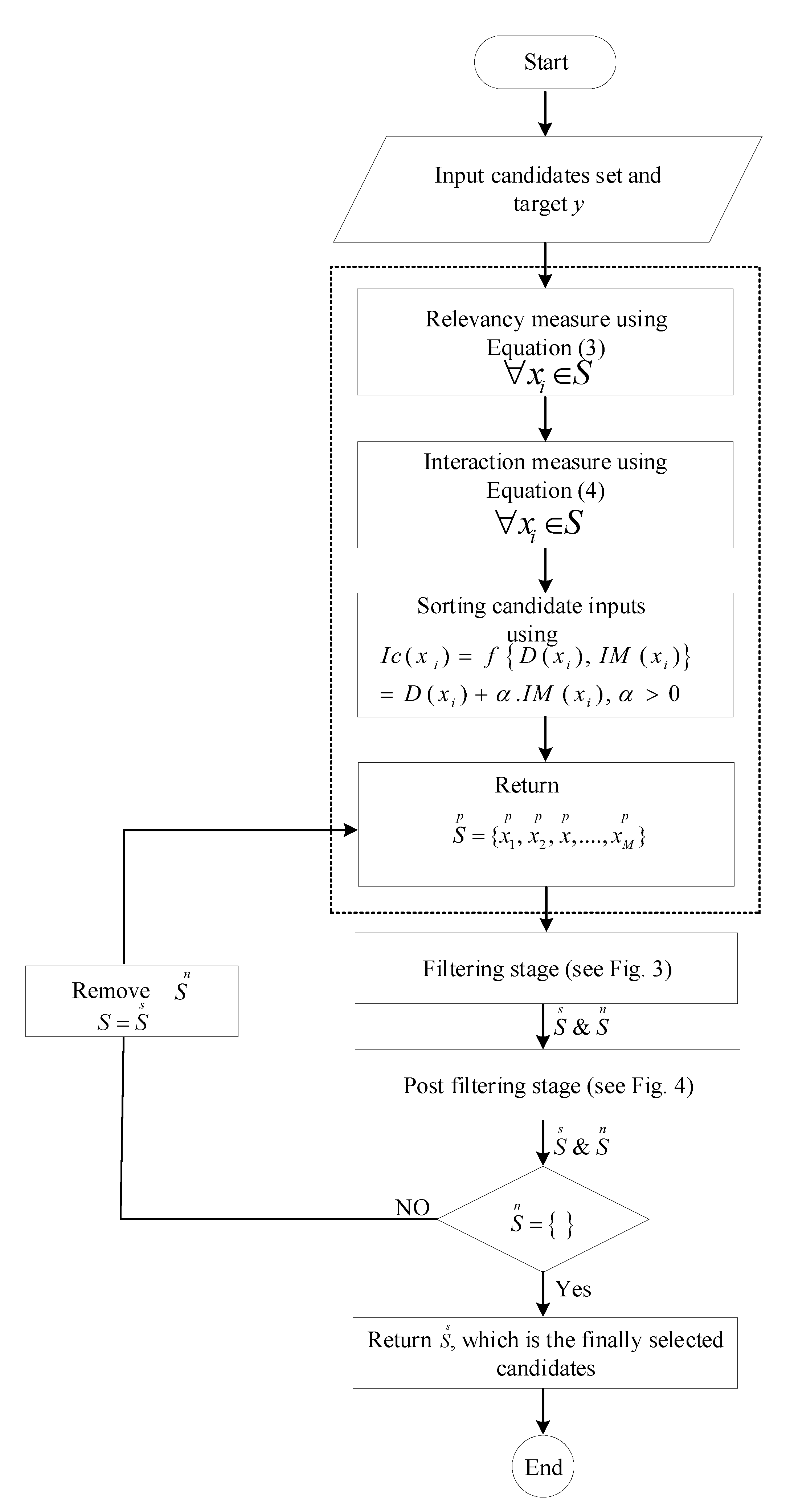
• The blocks enclosed in the dotted box in Figure 2 belong to the pre-filtering phase. In this phase, the relevancy and interaction measures are calculated, and candidate inputs are ranked based on the calculated measure.
• The information content can be measured from its individual information and the gained information using a modified version of Equation (4) mentioned in the flow chart in Figure 2. The function $f(,)$ is a monotonically increasing function, and $\alpha$ is a weight factor that weights the relevancy versus interaction measure. It can be adjusted and fine-tuned subject to the forecasting problem.
• The selected candidate inputs of the pre-filtering phase ($S^p$) are sorted in descending order based on the information content.

Step 3: Filtering phase individually depicted in Figure 3 and is described as follows:

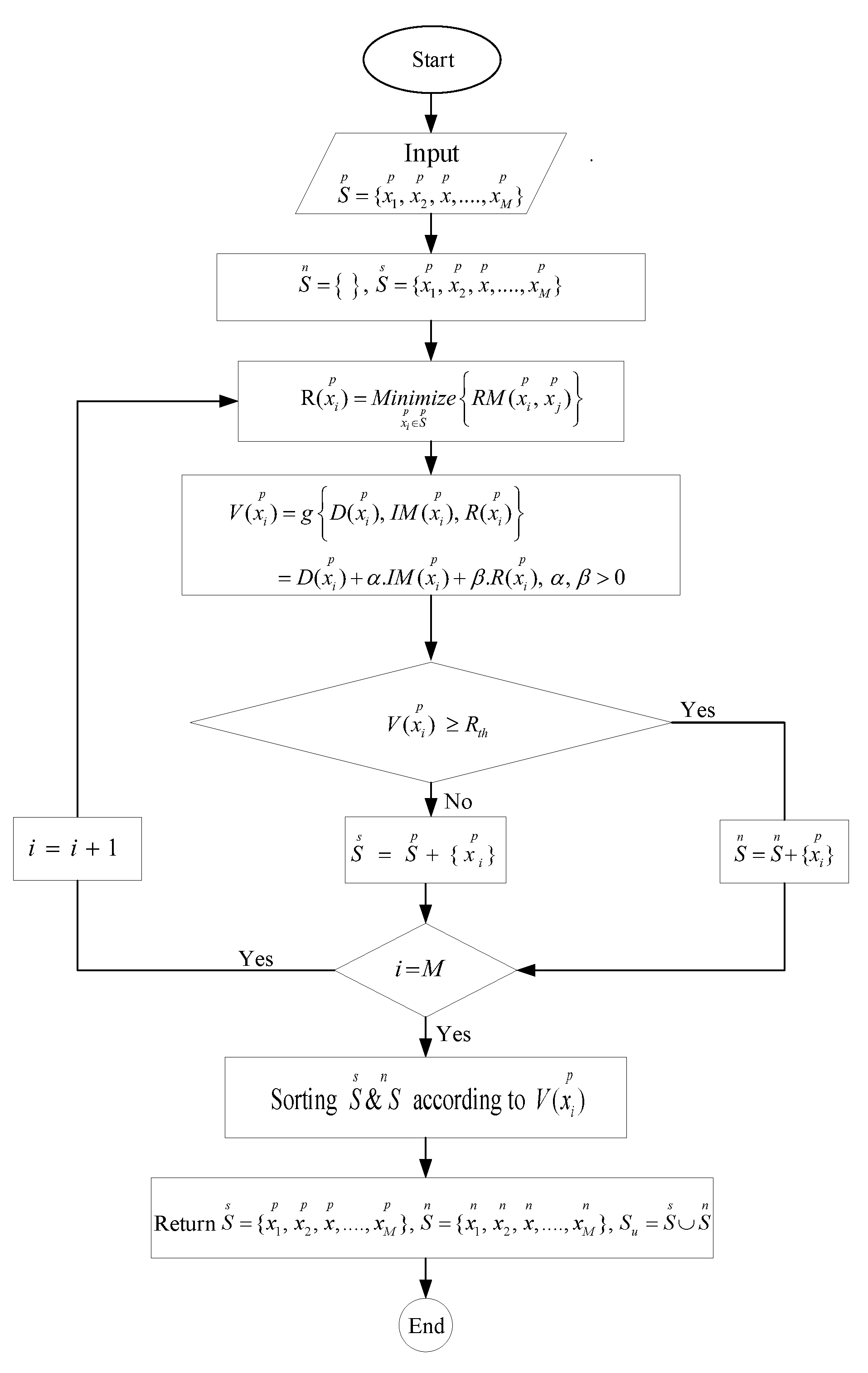
• The output of the pre-filtering phase is fed as an input to the filtering phase. In this step, the pre-selected features are partitioned into selected ($S^s$) and non-selected ($S^n$) features as shown in Figure 2. The redundancy measure is calculated by Equation (9) as:

  $$R(\stackrel{p}{x_i})=\underset{\stackrel{p}{x_i}\in \stackrel{p}{S}}{Minimize}\left\{RM(\stackrel{p}{x_i},\stackrel{p}{x_j})\right\},$$

  (9)

  where $R(\stackrel{p}{x_i})$ indicates the redundancy measure for each candidate input $\stackrel{p}{x_i}\in \stackrel{p}{S}$.
• The information value of candidate features is evaluated based on three measures: redundancy, relevancy, and interaction, which is mathematically described as:

  $$\begin{array}{cc}V(\stackrel{p}{x_i})\hfill & =g\left\{D(\stackrel{p}{x_i}),IM(\stackrel{p}{x_i}),R(\stackrel{p}{x_i})\right\}\hfill \\ & =D(\stackrel{p}{x_i})+\alpha .IM(\stackrel{p}{x_i})+\beta .R(\stackrel{p}{x_i}),\alpha ,\beta >0,\hfill \end{array}$$

  (10)

  where $V(\stackrel{p}{x_i})$ denotes information value, $g\left(,\right)$ indicates a monotonically increasing linear function, and $\beta$ denotes adjustable parameter, respectively.
• Decision about the information value is taken as follows:

  $$\begin{array}{c}\mathrm{If}V(\stackrel{p}{x_i})\ge R_{th}\to \stackrel{S}{S}=\stackrel{S}{S}+\{\stackrel{p}{x_i}\}\hfill \\ \mathrm{If}V(\stackrel{p}{x_i})\le R_{th}\to \stackrel{n}{S}=\stackrel{n}{S}+\{\stackrel{p}{x_i}\},\hfill \end{array}$$

  (11)

  where $R_{th}$ is the redundancy threshold. The information value is compared with the redundancy threshold; if it is greater than or equal to the redundancy threshold, then it will be put in the set of selected features list ($\stackrel{s}{S}$), otherwise it will be added in the set of non-selected features ($\stackrel{n}{S}$).
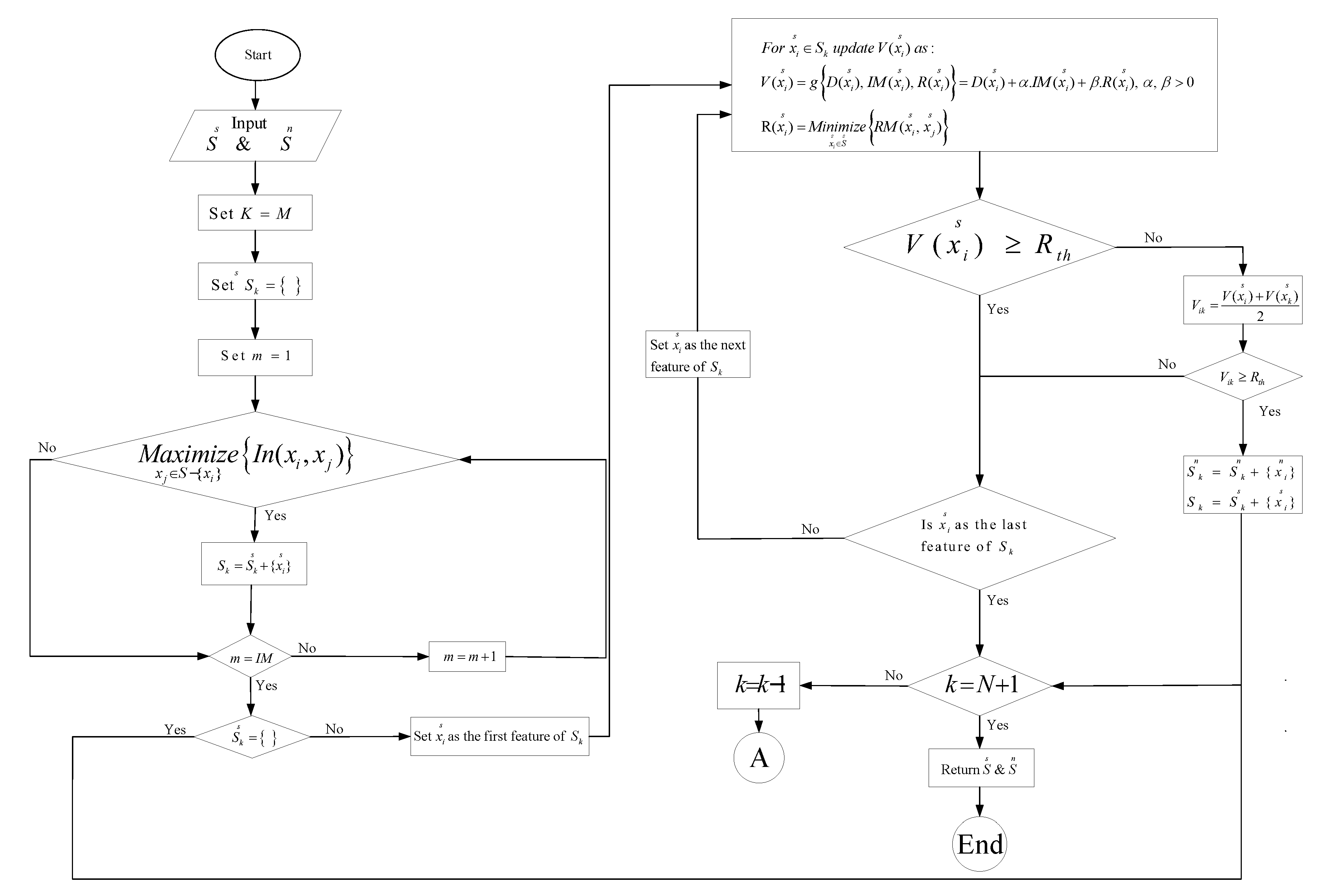
• The set of selected and non-selected features are sorted in descending order according to their information value and their union is also taken. The selected and non-selected feature sets and their union are given as input to the post-filtering stage, which is individually depicted in Figure 4.

Step 4: In the post-filtering phase, the selected ($\stackrel{s}{S}$) and non-selected inputs are modified and the information value $V(.)$ is updated. The updated information values are evaluated again using Equation (11) to transfer candidate inputs either to selected or non-selected features.

Step 5: The algorithm is terminated if the non-selected features set $\stackrel{n}{S}$ becomes null. The pre-filtering, filtering, and post-filtering phases are executed in each iteration and the execution never traps into an infinite loop. Finally, the selected features are fed into the forecaster module.

3.2. A Deep Learning FCRBM Model Based Forecasting Module

This module aims to devise a deep learning FCRBM-based forecaster, which is enabled through training to forecast future electrical energy consumption patterns. The discussion in Section 2 is ended with the conclusion that all forecasters in the literature can forecast non-linear electrical energy consumption patterns. Thus, a deep learning based FCRBM model among the intelligent forecasters is chosen because: (i) it forecasts non-linear electrical energy consumption pattern with reasonable accuracy and convergence speed, and (ii) it has scalable nature and has improved performance with scalability. The deep neural network FCRBM has a four layer structure with a particular number of neurons: (i) visible layer, (ii) hidden layer, (iii) style layer, and (iv) history layer. The FCRBM model is activated with the ReLU activation function and multivariate autoregressive algorithm to forecast the electrical energy consumption pattern. Both the ReLU activation function and multivariate autoregressive algorithm are chosen due to their fast convergence speed and they can overcome network issues such as vanishing gradient and overfitting. The ReLU is defined by Equation (12) as follows:

$$\begin{array}{c}f(x)=max(0,x)\hfill \\ f(x)\left\{\begin{array}{c}1\mathrm{if}x\ge 0\hfill \\ 0\mathrm{otherwise}.\hfill \end{array}\right.\hfill \end{array}$$

(12)

ReLU enables the FCRBM model to account for non-linearities and interactions. During the training process, to update weight and bias vectors, several algorithms are available in the literature, such as multivariate autoregressive algorithm [37], Levenberg-Marquardt algorithm [45], gradient descent and back-propagation [46]. Thus, among the training algorithms, a multivariate autoregressive algorithm is chosen because of its fast convergence speed and improved performance. The features selected in the data processing phase $\{S_1,S_2,S_3,\dots S_n\}$ are fed into the FCRBM-based forecaster module, where the first three-year data samples are used for the network training and the last one-year data samples are used for testing. The aim is to enable the deep learning based FCRBM model through a training process to forecast future electrical energy consumption patterns. The pictorial view of the training and learning process of the FCRBM model is illustrated in Figure 5. The FCRBM-based forecaster returns error signal, weights and biases, which are tuned by multivariate autoregressive algorithm [47]. This error signal returned from the forecaster module becomes the objective function of the optimization module for further improving the accuracy by optimizing the error signal.

3.3. The Proposed GWDO Algorithm-Based Optimization Module

The preceding deep learning FCRBM-based module returns the future forecasted electrical energy consumption pattern with some error, which is minimum according to the capability of the FCRBM model with ReLU and multivariate autoregressive algorithm. In order to further minimize error in the forecasted energy consumption pattern, the output of the FCRBM-based forecaster module is fed into our proposed GWDO-based optimization module. The aim of our proposed algorithm-based optimization module is to further minimize error in the forecasted energy consumption pattern. Thus, the optimization module takes error minimization as an objective function, which is modeled as follows:

$$\underset{R_{th},I_{th},C_i}{Minimize}Error(x)\forall x\in \{h,d\},$$

(13)

where $R_{th}$, $I_{th}$, and $C_i$ are redundancy, irrelevancy thresholds, and candidates interaction, respectively. The proposed GWDO-based module optimizes $R_{th}$, $I_{th}$, and $C_i$ and these parameters are fed to the data processing module. The feature selection technique in the data processing module uses optimized values of $R_{th}$, $I_{th}$ thresholds, and $C_i$ for optimal features selection. Joining the optimization module with the forecaster module increases the forecasting accuracy, while the convergence rate is degraded. The integration of optimization module with the forecaster module is usually done for such applications where the focus of the authors is on accuracy rather than convergence speed. To tune hyperparameters of forecaster, various parameter tuning techniques in the literature are proposed by authors such as heuristic techniques, convex programming, quadratic programming, linear and non-linear programming. Linear programming is not adopted in this study because the problem under consideration is non-linear. The non-linear programming are ignored due their increased execution time. The heuristic and convex optimization algorithms are rejected due to slow and premature convergence, respectively. The mEDE [37], enhanced differential evaluation (EDE) [48], and differential evaluation (DE) [45] among the evolutionary algorithms are refused due to the problems such as low precision, slow convergence, and getting stuck in local optimum [49], respectively. To remedy the problems of existing tuning algorithms, the GWDO algorithm is proposed to perform tuning of hyperparameters with fast converging speed. The proposed algorithm is a hybrid of WDO [21] and GA [50]. This hybrid algorithm is beneficial because it uses the key characteristics of both the algorithms. The WDO has fast convergence speed and GA enables a diversity of population. The forecasted electrical energy consumption pattern is fed into the utilization module to perform efficient energy management, planning, operation, and unit commitment in the SG.

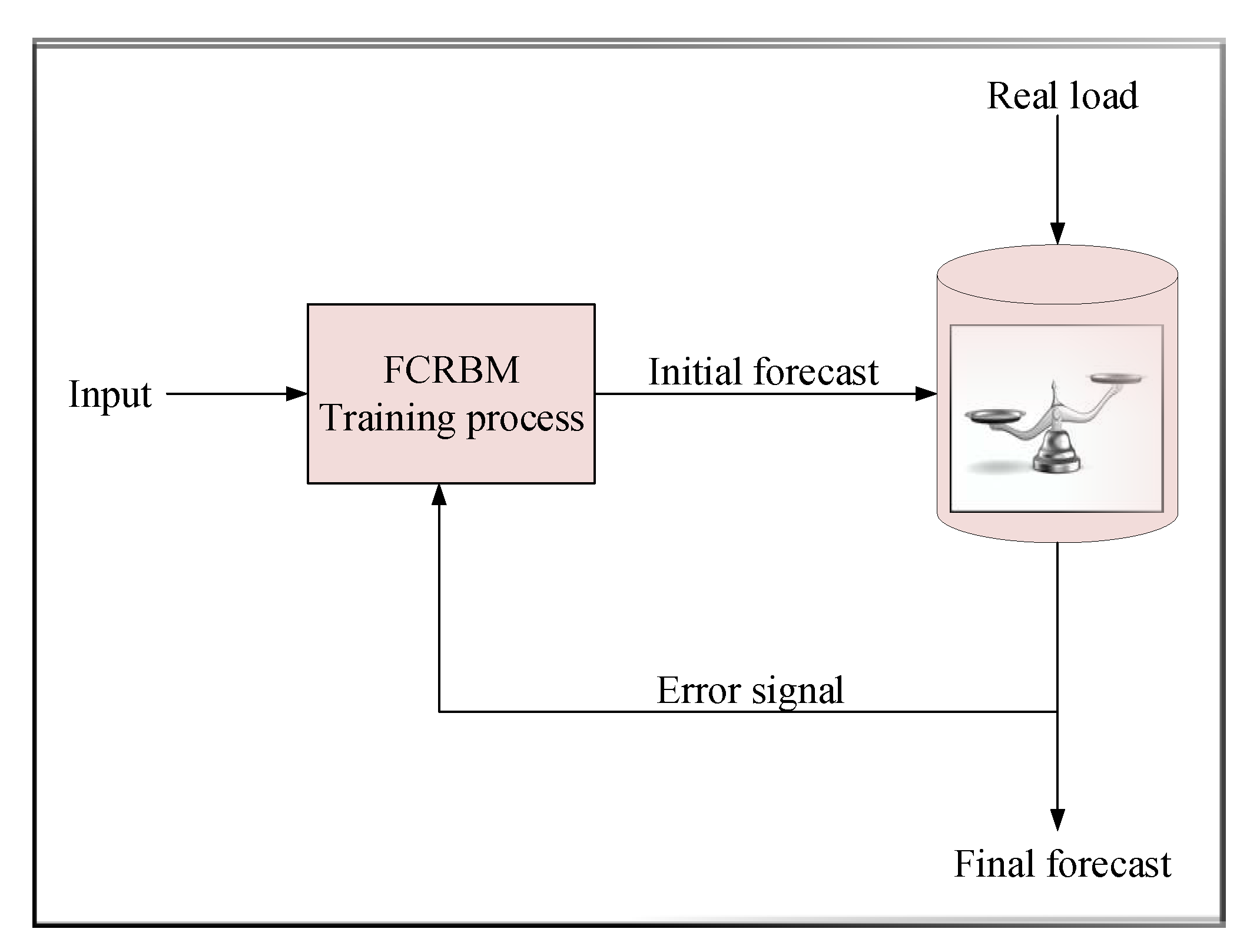
3.4. Utilization Module for Forecasting Results

The forecasted electrical energy consumption pattern is used for efficient energy management, long term planning and development of SG that need transmission and generation equipment, right of ways, state permits financing, substation construction, and power lines (distribution and transmission lines). Similarly, in [51], the authors used the potential of solar and wind energy mix for joint optimization of investment and operation of the microgrid. Moreover, the forecasting results based on the predicted period are classified into four categories: (i) very short-term, (ii) short-term, (iii) medium-term, and (iv) long-term. The very short-term forecasting results have prediction horizon from seconds/minutes to hours and are used for flow control and day-to-day operations in the SG. The short-term electrical energy consumption forecasting results have forecasting horizon from hours to weeks and are used for evaluation of net interchange, scheduling functions, unit commitment, and system security analysis. Moreover, forecasting results are vital for managing generation and demand and energy management in the electricity market of the SG. The medium forecasting results cover weeks to months’ prediction horizon and are used by the electrical power company for maintenance planning, fuel scheduling, and hydro reservoir management. These forecasting results are also used for power grid capacity planning, maintenance scheduling, and power grid ongoing operations to facilitate efficient management of energy resources. The long-term forecasting results horizon is typically more than one year and is vital for major strategic decisions, such as market environmental factors, opportunities, development, infrastructure planning, and internal resources to be taken within the electricity market. Thus, electric power companies need to develop the forecasting model that can identify forecasting problems and based on this, predict for one of the four forecasting time horizons. These forecasting models provide strong support to the electric power companies to use forecasting results to achieve the said objectives.

4. Simulations Results, Performance Evaluation, and Discussion

To test and evaluate the efficacy of the proposed FS-FCRBM-GWDO framework, simulations are conducted in MATLAB 2018, which is installed on a laptop having specifications of Intel(R) Corei3-CPU @2.4GHz, and 6GB RAM with Microsoft Windows 10. FS-FCRBM-GWDO is evaluated in comparison with existing frameworks: MI-mEDE-ANN [36], AFC-STLF [37], Bi-level [45], and FS-ANN [52]. These existing hybrid frameworks are chosen as benchmark frameworks due to the architectural resemblance with the proposed FS-FCRBM-GWDO framework. However, the FS-FCRBM-GWDO framework and the selected benchmark frameworks have different complexities because the focus of the authors is on different objectives such as accuracy, convergence rate, and stability. FS-FCRBM-GWDO is tested on real-time FE power grid hourly energy consumption data of USA. The dataset is taken from publicly available PJM electricity market [53]. The same dataset is also considered in [37]. The monthly electrical energy consumption data of the FE power grid of USA for the years 2014–2017 is depicted in Figure 6. The data is for four years. The 80% data is used to train the FCRBM deep learning model and 20% data is used for testing the FCRBM model. The control parameters used in simulations are listed in

Table 2. Simulation parameters.

Control Parameters	Value
Hidden layer	1
Neurons in hidden	10
Output layer	1
Number of output neurons	1
Number of epochs	100
Number of iterations	100
Learning rate	$0.0019$
Momentum	0.6
Initial weight	0.1
Initial bias	0
Max	0.9
Min	0.1
Decision variables	2
Population size	24
Delay of weight	0.0002
Historical load data	4 years
Exogenous parameters	4 years

and can be justified from [37]. The control parameters listed in Table 2 are kept the same for both the proposed and benchmark models subjected to a fair comparative analysis. The proposed FS-FCRBM-GWDO framework is evaluated in terms of two performance metrics: (i) accuracy (MAPD, variance (${\sigma }^2$), correlation coefficient (R)), and (ii) convergence speed (execution time, convergence rate). The mathematical modeling of the performance metrics is as follows:

$$MAPD=\left(\frac{1}{\tau }\sum _{t=1}^{\tau }\frac{|R_t-F_t|}{|R_t|}\right)\times 100,$$

(14)

$${\sigma }^2=\frac{1}{\tau }\sum _{t=1}^{\tau }\left(R_t-F_t\right),$$

(15)

$$R=\frac{\mathrm{E}\{(R_t-{\mu }_R)(F_t-{\mu }_F)\}}{\sqrt{\sum {(R_t-{\mu }_R)}^2\times \sum {(F_t-{\mu }_F)}^2}},$$

(16)

where $R_t$ and $F_t$ represent the real and forecasted load at time t, and ${\mu }_R$ and ${\mu }_F$ represent the mean of real and forecasted electrical energy consumption, respectively. Equation (14) represents the MAPD performance metric, Equation (15) represents the variance ${\sigma }^2$ metric, and Equation (16) represents the correlation coefficient metric, respectively.

The first three performance metrics (Equations (14)–(16)) are for accuracy analysis, which is calculated as:

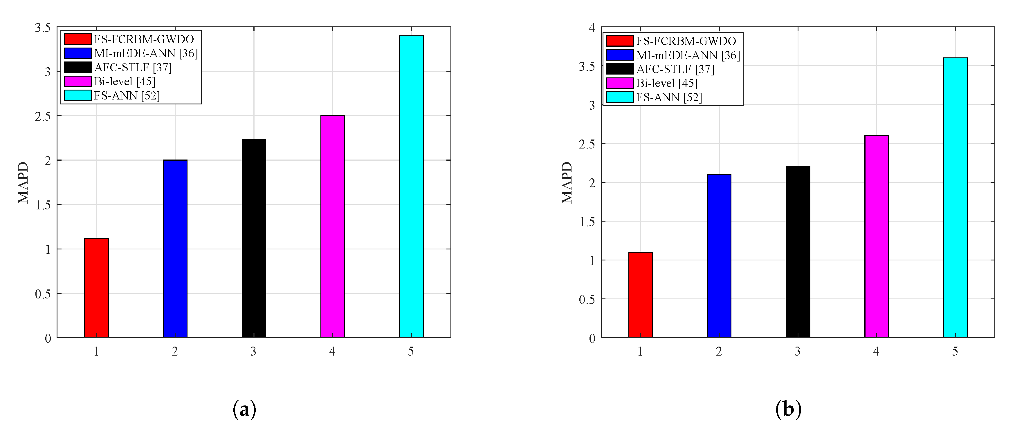
• Accuracy = 100 − MAPD(x).

The convergence speed is defined in terms of execution time and convergence rate as:

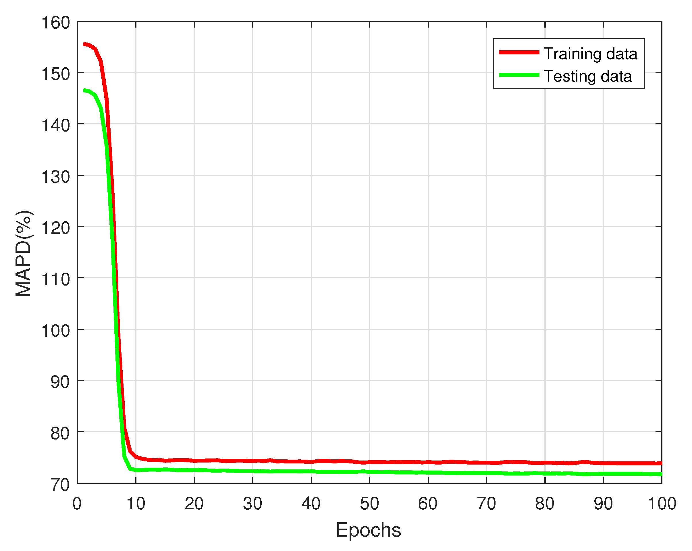
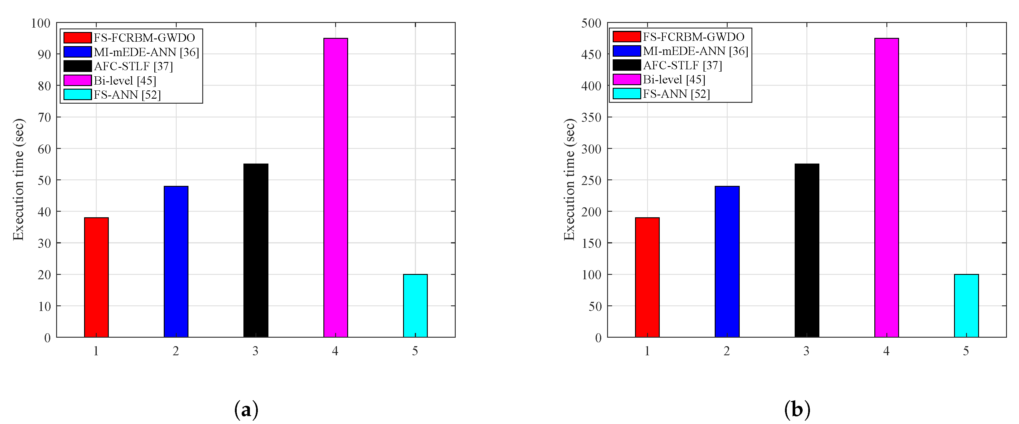
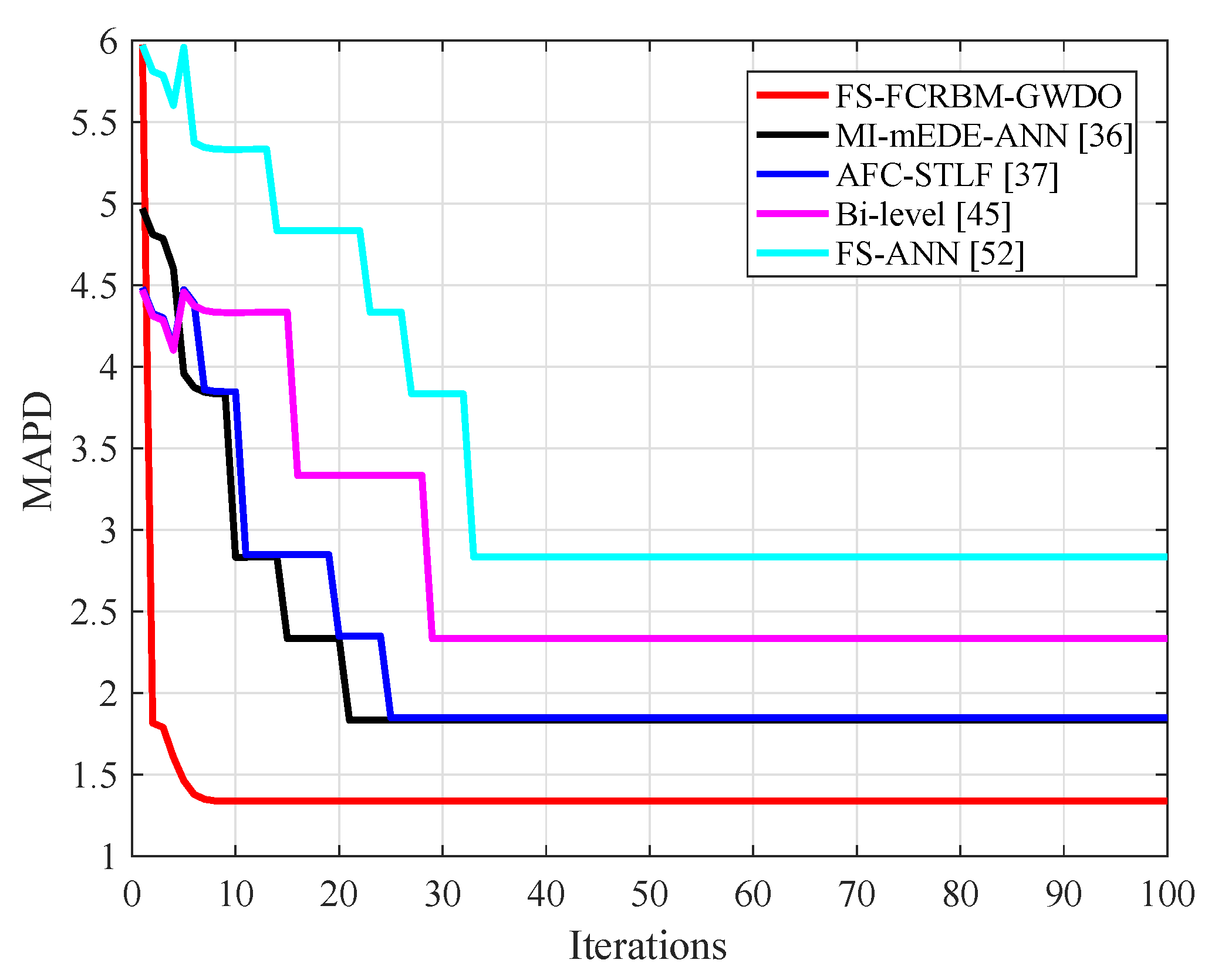
• Convergence speed corresponds to the execution time and the convergence rate: (i) execution time is the time taken by the forecasting model to return future electrical energy consumption pattern; and (ii) convergence rate is the rate at which the model converges to a particular epoch where its performance saturates and the error does not reduce any further with increase in the number of epochs. The forecasting models that have low execution time and converge at earlier epochs are considered fast. In this research, the execution time is measured in seconds, and the convergence rate is measured in terms of number of epochs.

A detailed discussion on the proposed hybrid FS-FCRBM-GWDO framework and benchmark frameworks in terms of performance metrics is as follows:

4.1. Proposed Model’s Learning Evaluation

A learning evaluation compares a model’s performance for testing and training data samples across some epochs to ensure whether the model is memorizing data or learning from data. The learning curve is bad when the model has high variance and bias, which indicates that the model is memorizing data rather than learning. The model with high variance and bias leads to reduced accuracy and poor generalization. The learning curve for the deep learning FCRBM model is good due to two reasons: (i) there is no variance and bias because the difference between training and testing errors is minimum, and (ii) both testing and training errors decrease with increase in the number of epochs. The learning curve of FCRBM model is depicted in Figure 7. At the start, the MAPD is high when the number of epochs is zero, which indicates that the model is not well-trained. When the number of epochs increases, the MAPD decreases and converges to a minimum acceptable value. This point is called the saturation point and it indicates that the model is well-trained.

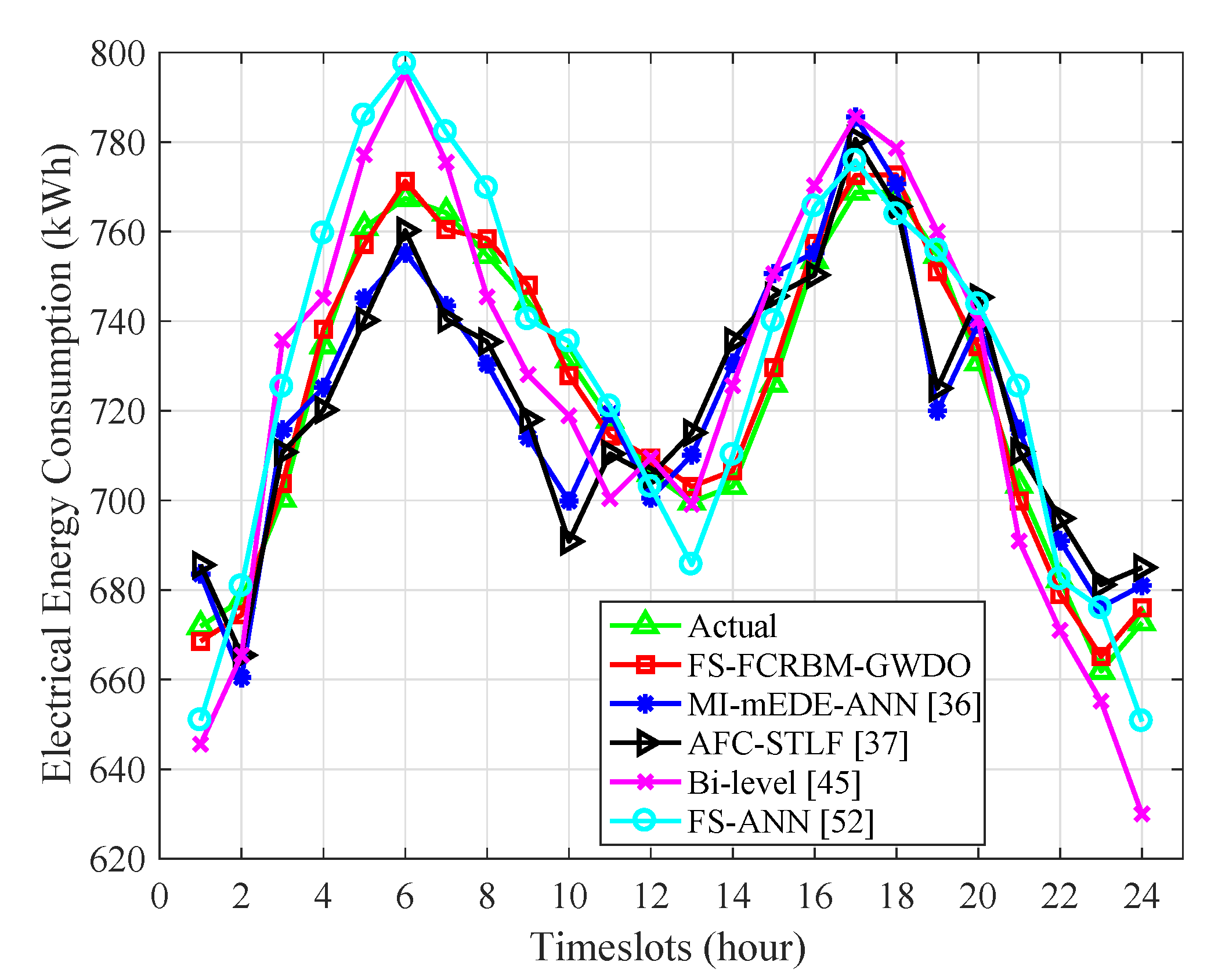
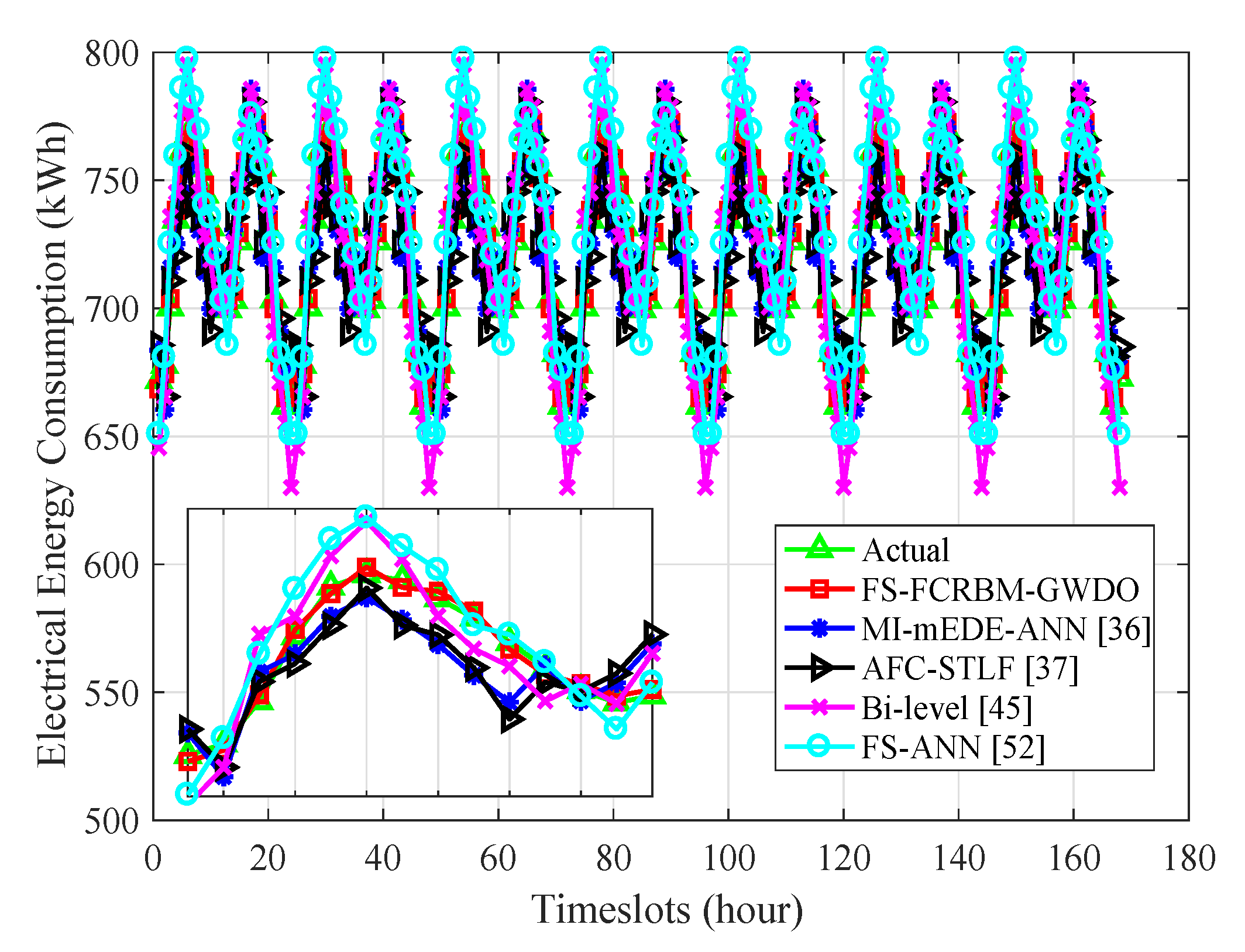
4.2. Day Ahead Electrical Energy Consumption Forecasting With Hour Resolution

The evaluation of day ahead forecasted electrical energy consumption in the FE power grid of the proposed FS-FCRBM-GWDO framework in comparison to the benchmark frameworks such as FS-ANN, AFC-STLF, Bi-level, and MI-mEDE-ANN is depicted in Figure 8. Moreover, the accuracy analysis in terms of MAPD, variance, and correlation coefficient for the proposed and existing models are listed in

Table 3. FE power grid February results of leap year 2016: comparative performance evaluation of the proposed and existing models in terms of MAPD, variance, and correlation coefficient.

	Electrical Energy Consumption Forecasting Models
Day	FS-FCRBM-GWDO			MI-mEDE-ANN			AFC-STLF			Bi-Level			FS-ANN
	MAPD	${\mathit{\sigma }}^2$	R	MAPD	${\mathit{\sigma }}^2$	R	MAPD	${\mathit{\sigma }}^2$	R	MAPD	${\mathit{\sigma }}^2$	R	MAPD	${\mathit{\sigma }}^2$	R
1	1.12	1.13	0.70	2.20	1.55	0.50	2.30	1.60	0.52	2.60	1.75	0.44	3.30	1.90	0.44
2	1.10	0.98	0.68	2.10	1.45	0.58	2.15	1.55	0.56	2.80	1.73	0.46	3.35	1.80	0.36
3	1.09	1.10	0.71	2.50	1.30	0.51	2.10	1.48	0.53	2.75	1.65	0.43	3.20	1.83	0.33
4	1.03	0.97	0.80	2.02	1.20	0.50	2.40	1.49	0.54	2.85	1.75	0.44	3.40	1.85	0.34
5	1.50	1.09	0.65	2.10	1.15	0.55	2.25	1.37	0.55	2.87	1.65	0.45	3.15	1.78	0.35
6	1.30	1.07	0.75	2.30	1.34	0.65	2.15	1.35	0.69	2.89	1.69	0.59	3.25	1.95	0.49
7	1.24	1.04	0.69	2.11	1.55	0.60	2.10	1.60	0.65	2.75	1.68	0.44	3.67	1.80	0.34
8	1.23	1.02	0.70	2.15	1.45	0.50	2.09	1.65	0.55	2.70	1.77	0.55	3.55	1.83	0.45
9	1.08	1.05	0.80	2.35	1.36	0.55	2.50	1.66	0.56	2.65	1.71	0.56	3.45	1.79	0.46
10	1.05	0.99	0.79	2.40	1.39	0.69	2.44	1.67	0.60	2.63	1.78	0.65	3.10	1.87	0.55
11	1.15	1.10	0.87	2.01	1.45	0.77	2.35	1.55	0.75	2.70	1.65	0.35	3.15	1.85	0.45
12	1.25	1.11	0.65	2.06	1.50	0.55	2.12	1.58	0.55	2.60	1.66	0.45	3.59	1.77	0.35
13	1.10	0.96	0.81	2.10	1.55	0.71	2.20	1.43	0.75	2.63	1.69	0.25	3.33	1.69	0.35
14	1.12	0.99	0.79	2.12	1.37	0.75	2.23	1.47	0.70	2.36	1.75	0.40	3.39	1.59	0.30
15	1.10	1.03	0.78	2.13	1.46	0.78	2.27	1.30	0.73	2.50	1.59	0.43	3.54	1.89	0.53
16	1.18	1.05	0.79	2.00	1.39	0.70	2.13	1.35	0.78	2.58	1.67	0.58	3.23	1.88	0.48
17	1.19	1.08	0.80	2.13	1.48	0.60	2.35	1.55	0.65	2.56	1.70	0.55	3.28	1.79	0.50
18	1.21	1.09	0.85	2.19	1.29	0.85	2.10	1.36	0.64	2.65	1.72	0.54	3.92	1.85	0.44
19	1.25	1.12	0.90	2.16	1.36	0.50	2.14	1.55	0.59	2.54	1.58	0.59	3.53	1.75	0.44
20	1.44	0.95	0.67	2.17	1.47	0.60	2.15	1.45	0.48	2.50	1.65	0.58	3.22	1.69	0.48
21	1.39	0.90	0.71	2.34	1.51	0.58	2.19	1.54	0.58	2.59	1.72	0.48	3.27	1.88	0.38
22	1.17	0.99	0.75	2.10	1.50	0.75	2.10	1.40	0.59	2.80	1.63	0.49	3.60	1.80	0.39
23	1.15	1.01	0.86	2.30	1.45	0.64	2.13	1.34	0.39	2.75	1.65	0.59	3.23	1.71	0.49
24	1.08	1.07	0.87	2.01	1.34	0.73	2.24	1.60	0.58	2.65	1.53	0.48	3.89	1.74	0.38
26	1.05	1.05	0.90	2.00	1.56	0.09	2.26	1.61	0.49	2.85	1.59	0.59	3.65	1.63	0.49
27	1.03	1.10	0.88	2.10	1.40	0.58	2.10	1.48	0.77	2.55	1.68	0.57	3.83	1.80	0.47
28	1.25	1.11	0.76	2.09	1.35	0.56	2.15	1.50	0.58	2.60	1.75	0.48	3.35	1.79	0.38
29	1.27	1.13	0.77	2.08	1.32	0.55	2.13	1.53	0.59	2.62	1.76	0.49	3.36	1.78	0.39
Avg.	1.10	1.03	0.79	2.20	1.25	0.65	2.10	1.35	0.60	2.60	1.72	0.55	3.60	1.80	0.45

. The results clearly indicate that the proposed FS-FCRBM-GWDO framework forecasts the day-ahead electrical energy consumption of the FE power grid. All the forecasters (proposed and benchmark) are capable of learning the non-linearities of historical energy consumption time series data. The non-linear forecasting ability is due to the use of non-linear activation functions such as tangent hyperbolic (Tanh), sigmoidal, and ReLU. The benchmark frameworks (FS-ANN, AFC-STLF, Bi-level, and MI-mEDE-ANN) use the sigmoid activation function, whereas the proposed hybrid FS-FCRBM-GWDO model uses ReLU and multivariate autoregressive algorithm because they have fast converging speed and solve the problems of vanishing gradient and overfitting. Figure 8 illustrates that the energy consumption pattern forecasted by the proposed framework closely follows the actual energy consumption pattern as compared to the benchmark models (FS-ANN, AFC-STLF, Bi-level, and MI-mEDE-ANN). It is listed in Table 3 that the MAPD of the proposed FS-FCRBM-GWDO framework is 1.10%, whereas the MAPD of AFC-STLF, MI-mEDE-ANN, FS-ANN, and Bi-level is 2.1%, 2.2%, 3.6%, 2.6% respectively. Thus, it is obvious from Figure 8 and Table 3 that the proposed hybrid FS-FCRBM-GWDO model performs better than the benchmark frameworks in terms of accuracy.

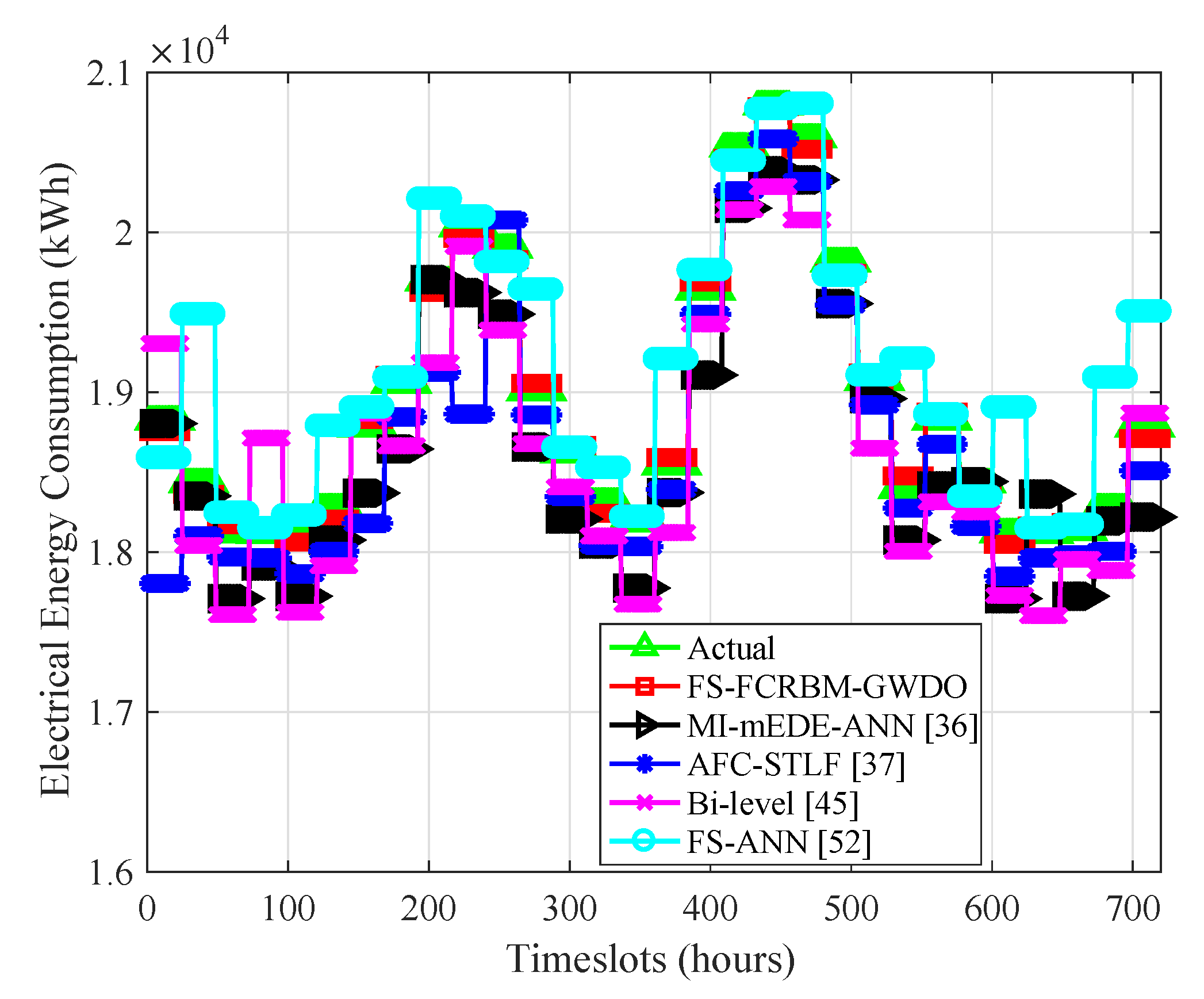
4.3. Electrical Energy Consumption Forecasting for Week and Month Ahead of Time Horizon with Hour Resolution

The week ahead electrical energy consumption forecasting with hour resolution for the proposed and existing models of the FE power grid is depicted in Figure 9. It is important to note that the proposed hybrid FS-FCRBM-GWDO model has fast, stable, and accurate electrical energy consumption forecasting as compared to the benchmark frameworks (FS-ANN, AFC-STLF, Bi-level, and MI-mEDE-ANN). FS-FCRBM-GWDO-based forecasted energy consumption curve closely follows the actual energy consumption, which is illustrated in the zoomed box of Figure 9. The statistical results of accuracy in terms of MAPD for the proposed hybrid FS-FCRBM-GWDO model is 1.12%, whereas the MAPD of FS-ANN is 3.4%, MI-mEDE-ANN is 2.23%, Bi-level is 2.5%, and AFC-STLF is 2.0%. The reason for this superior performance of our proposed model is due to the use of deep learning based FCRBM model with ReLU, multivariate autoregressive algorithm, and GWDO algorithm-based optimization module. Similarly, the month ahead of electrical energy consumption forecasting with hour resolution is illustrated in Figure 10 and Table 3. The proposed FS-FCRBM-GWDO model-based month ahead forecasting curve closely follows the target curve, which ensures the superior performance of the proposed model as compared to the benchmark models. The performance evaluation of the proposed FS-FCRBM-GWDO model and the benchmark models for the leap year 2016 with the month resolution in terms of MAPD, variance, and correlation coefficient is presented in

Table 4. FE power grid results of the leap year 2016: comparative performance analysis of the FS-FCRBM-GWDO and existing models in terms of MAPD, correlation coefficient and variance.

	Electrical Energy Consumption Forecasting Models
Month	FS-FCRBM-GWDO			MI-mEDE-ANN			AFC-STLF			Bi-Level			FS-ANN
	MAPD	${\mathit{\sigma }}^2$	R	MAPD	${\mathit{\sigma }}^2$	R	MAPD	${\mathit{\sigma }}^2$	R	MAPD	${\mathit{\sigma }}^2$	R	MAPD	${\mathit{\sigma }}^2$	R
1	1.10	1.03	0.78	2.13	1.46	0.78	2.27	1.30	0.73	2.50	1.59	0.43	3.54	1.89	0.53
2	1.44	0.95	0.67	2.17	1.47	0.60	2.15	1.45	0.48	2.50	1.65	0.58	3.22	1.69	0.48
3	1.25	1.11	0.65	2.06	1.50	0.55	2.12	1.58	0.55	2.60	1.66	0.45	3.59	1.77	0.35
4	1.03	0.97	0.80	2.02	1.20	0.50	2.40	1.49	0.54	2.85	1.75	0.44	3.40	1.85	0.34
5	1.19	1.08	0.80	2.13	1.48	0.60	2.35	1.55	0.65	2.56	1.70	0.55	3.28	1.79	0.50
6	1.15	1.01	0.86	2.30	1.45	0.64	2.13	1.34	0.39	2.75	1.65	0.59	3.23	1.71	0.49
7	1.24	1.04	0.69	2.11	1.55	0.60	2.10	1.60	0.65	2.75	1.68	0.44	3.67	1.80	0.34
8	1.23	1.02	0.70	2.15	1.45	0.50	2.09	1.65	0.55	2.70	1.77	0.55	3.55	1.83	0.45
9	1.25	1.11	0.65	2.06	1.50	0.55	2.12	1.58	0.55	2.60	1.66	0.45	3.59	1.77	0.35
10	1.18	1.05	0.79	2.00	1.39	0.70	2.13	1.35	0.78	2.58	1.67	0.58	3.23	1.88	0.48
11	1.15	1.10	0.87	2.01	1.45	0.77	2.35	1.55	0.75	2.70	1.65	0.35	3.15	1.85	0.45
12	1.21	1.09	0.85	2.19	1.29	0.85	2.10	1.36	0.64	2.65	1.72	0.54	3.92	1.85	0.44
Avg.	1.10	1.03	0.79	2.20	1.25	0.65	2.10	1.35	0.60	2.60	1.72	0.55	3.60	1.80	0.45

.

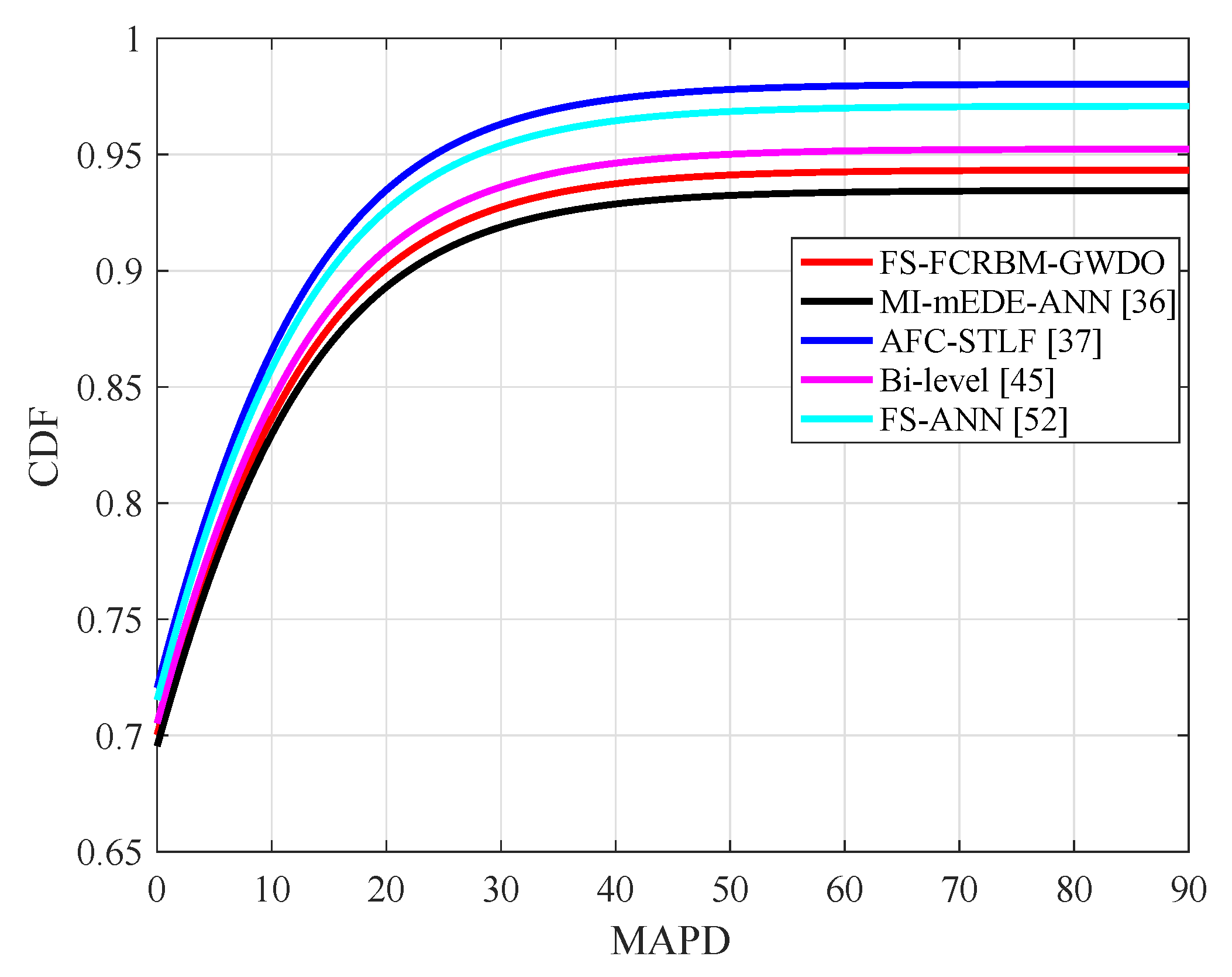
4.4. Performance Analysis of Proposed FS-FCRBM-GWDO Model in Terms of Convergence Speed and MAPD

The statistical evaluation of the accuracy, execution time, and convergence speed of the proposed and benchmark models is depicted in Figure 11, Figure 12 and Figure 13, respectively. The MAPD is a measure of deviation of the predicted value from the actual value. The smaller MAPD indicates high accuracy while the larger MAPD value represents the worst accuracy. The accuracy analysis in terms of MAPD for the day ahead and week ahead time horizon is depicted in Figure 11a,b, respectively. The MAPD of the proposed FS-FCRBM-GWDO model is 1.10%, whereas the MAPD values of FS-ANN, AFC-STLF, MI-mEDE-ANN, and Bi-level are 3.6%, 2.23%, 2.2%, and 2.6%, respectively. From the above performance evaluations and discussion, we come to the conclusion that a Bi-level model is better than the FS-ANN model in terms of MAPD metrics. The reason for this accurate performance is the integration of DE based optimization module with the forecaster module. However, the MAPD is reduced by integrating the optimization module while the execution time is increased, as depicted in Figure 13. The figure illustrates that the execution time increases from 20s to 95s with the integration of the optimization module. Thus, we conclude that a tradeoff exists between the accuracy and the convergence rate. Hence, the proposed hybrid FS-FCRBM-GWDO model comparatively reduces the execution time because of the following reasons: (i) fast converging GWDO [20] is used for optimization instead of EDE and mEDE [37,48], (ii) ReLU and multivariate autoregressive algorithm are used instead of sigmoidal activation function, (iii) the deep learning FCRBM model is used, which is more effective than the simple ANN, (iv) the data pre-processing, i.e., cleansing and normalization operation (see Equation (1)) is used, and (v) for feature selection, a novel concept of feature interaction is introduced to redundancy and irrelevancy filters (see Section 3.1), while the benchmark models only use mutual information-based redundancy and irrelevancy filters. These modifications are devised in the benchmark models (MI-mEDE-ANN, AFC-STLF, and Bi-level), which lead to a reduced execution time of 38s. Moreover, the accuracy of the proposed hybrid FS-FCRBM-GWDO model is also improved compared to the benchmark models (FS-ANN, AFC-STLF, Bi-level, and MI-mEDE-ANN) (See Figure 11). However, the proposed FS-FCRBM-GWDO framework takes more time to execute as compared to FS-ANN due to the absence of the optimization module with the FS-ANN model (See Figure 13).

To show the fast convergence and effective searchability of the proposed hybrid FS-FCRBM-GWDO model, the performance analysis in terms of convergence speed for 100 iterations in comparison with benchmark models such as FS-ANN, Bi-level, AFC-STLF, and MI-mEDE-ANN, is depicted in Figure 13. For all models (proposed and existing), the MAPD decreases as the number of iterations increases. However, the proposed model converges around the 10th iteration, which shows its fast convergence and effective searchability, while the benchmark models, FS-ANN, Bi-level, AFC-STLF, and MI-mEDE-ANN, converge around 33th, 29th, 25th, and 21th, iterations, respectively. Accordingly, the proposed GWDO algorithm can be a more appropriate approach when used for optimization in integrated frameworks. For the convergence analysis, just the MAPD performance metric is depicted here for the proposed and existing models.

Analysis of the proposed hybrid FS-FCRBM-GWDO model and benchmark models such as FS-ANN, Bi-level, AFC-STLF, and MI-mEDE-ANN in terms of cumulative distribution function (CDF) of error is illustrated in Figure 14. FS-FCRBM-GWDO model is superior in terms of CDF as compared to the existing models. The deep learning FCRBM model provides reliable forecasting even in the highly uncertain situation because the layout of the deep layers can capture the key features. Thus, our proposed FS-FCRBM-GWDO framework would be a better choice for the distribution system operators for efficient and effective energy management of the SG. The overall evaluation of the FS-FCRBM-GWDO framework and the existing frameworks such as FS-ANN, Bi-level, AFC-ANN, and MI-mEDE-ANN in terms of computational complexity, execution time, convergence rate, and accuracy is listed in

Table 5. Evaluation of the proposed FS-FCRBM-GWDO framework and the benchmark frameworks such as FS-ANN, Bi-level, AFC-ANN, and MI-mEDE-ANN in terms of computational complexity, execution time, convergence rate, and accuracy.

Performance Parameters	Electrical Energy Consumption Forecasting Models
	FS-ANN	Bi-Level	AFC-STLF	MI-mEDE-ANN	FS-FCRBM-GWDO
Computational complexity (level)	Low	High	Moderate	High	Moderate
Convergence rate (epochs)	33th	29th	25th	21th	10th
Execution time (sec)	20	95	56	48	38
Accuracy (%)	96.4	97.4	97.9	97.8	98.9

. Thus, from the above simulation results, performance analysis, and discussions, we come to the conclusion that the proposed hybrid FS-FCRBM-GWDO model outperforms the benchmark models such as MI-mEDE-ANN [36], AFC-STLF [37], Bi-level [45], and FS-ANN [52] in terms of convergence rate, accuracy, computational complexity, and execution time.

5. Conclusions

Electrical energy consumption forecasting is imperative for the decision-making activities of the SG such as efficient use of available energy, operation planning, load scheduling, and contract evaluation. In this regard, a novel hybrid electrical energy consumption forecasting model is proposed to provide accurate and efficient forecasting with an affordable convergence rate. The proposed model is an integrated framework of FS, FCRBM-based forecaster, and GWDO-based optimizer, known as FS-FCRBM-GWDO. In the proposed model, a novel concept of features interaction is developed in addition to relevancy and redundancy filters of the MI technique to select key features for FCRBM-based forecaster. Keeping in view the non-linearity and complexity of the investigated problem, a GWDO algorithm is proposed for the optimization module of the proposed model to further improve accuracy with reasonable convergence of the forecasting results returned from the FCRBM-based forecaster. The proposed FS-FCRBM-GWDO model is examined on FE power grid data of USA in terms of MAPD, variance, correlation coefficient, and convergence rate. Simulation results validated that the proposed FS-FCRBM-GWDO model achieved 98.9% accuracy, which is better than the benchmark models, such as MI-mEDE-ANN (97.8%), AFC-STLF (97.9%), Bi-level (97.4%), and FS-ANN (96.4%), respectively. The proposed model reduced the average execution time by 20.8%, 32.1%, and 60% when compared to MI-mEDE-ANN, AFC-STLF, and Bi-level, respectively. It is concluded that our proposed FS-FCRBM-GWDO model outperformed benchmark electrical energy consumption forecasting models in terms of both accuracy and convergence rate.

In the future, this work can be extended for energy management applications of smart cities by integrating Internet of things (IoT) with data analytic models. Another future direction is the addition of sensors with deep learning models to promote data analytic applications in the field of SG.

References

1. Hafeez, G.; Alimgeer, K.S.; Wadud, Z.; Khan, I.; Usman, M.; Qazi, A.B.; Khan, F.A. An Innovative Optimization Strategy for Efficient Energy Management with Day-ahead Demand Response Signal and Energy Consumption Forecasting in Smart Grid using Artificial Neural Network. IEEE Access 2020. [Google Scholar] [CrossRef]
2. Zhang, X.; Wang, J.; Zhang, K. Short-term electric load forecasting based on singular spectrum analysis and support vector machine optimized by Cuckoo search algorithm. Electr. Power Syst. Res. 2017, 146, 270–285. [Google Scholar] [CrossRef]
3. Lin, C.; Chou, L. A novel economy reflecting short-term load forecasting approach. Energy Convers. Manag. 2013, 65, 331–342. [Google Scholar] [CrossRef]
4. Al-Hamadi, H.M.; Soliman, S.A. Short-term electric load forecasting based on Kalman filtering algorithm with moving window weather and load model. Electr. Power Syst. Res. 2004, 68, 47–59. [Google Scholar] [CrossRef]
5. Sudheer, G.; Suseelatha, A. Short term load forecasting using wavelet transform combined with Holt–Winters and weighted nearest neighbor models. Int. J. Electr. Power Energy Syst. 2015, 64, 340–346. [Google Scholar] [CrossRef]
6. Akay, D.; Atak, M. Grey prediction with rolling mechanism for electricity demand forecasting of Turkey. Energy 2007, 32, 1670–1675. [Google Scholar] [CrossRef]
7. Song, K.; Baek, Y.; Hong, D.H.; Jang, G. Short-term load forecasting for the holidays using fuzzy linear regression method. IEEE Trans. Power Syst. 2005, 20, 96–101. [Google Scholar] [CrossRef]
8. Guo, Y.; Nazarian, E.; Ko, J.; Rajurkar, K. Hourly cooling load forecasting using time-indexed ARX models with two-stage weighted least squares regression. Energy Convers. Manag. 2014, 80, 46–53. [Google Scholar] [CrossRef]
9. Felice, M.D.; Alessandri, A.; Catalano, F. Seasonal climate forecasts for medium-term electricity demand forecasting. Appl. Energy 2015, 137, 435–444. [Google Scholar] [CrossRef]
10. Sousa, J.C.; Neves, L.P.; Jorge, H.M. Assessing the relevance of load profiling information in electrical load forecasting based on neural network models. Int. J. Electr. Power Energy Syst. 2012, 40, 85–93. [Google Scholar] [CrossRef]
11. Mori, H.; Yuihara, A. Deterministic annealing clustering for ANN-based short-term load forecasting. IEEE Trans. Power Syst. 2001, 16, 545–551. [Google Scholar] [CrossRef]
12. Zeng, N.; Zhang, H.; Liu, W.; Liang, J.; Alsaadi, F.E. A switching delayed PSO optimized extreme learning machine for short-term load forecasting. Neurocomputing 2017, 240, 175–182. [Google Scholar] [CrossRef]
13. Xia, C.; Wang, J.; McMenemy, K. Short, medium and long term load forecasting model and virtual load forecaster based on radial basis function neural networks. Int. J. Electr. Power Energy Syst. 2010, 32, 743–750. [Google Scholar] [CrossRef] [Green Version]
14. Li, H.; Guo, S.; Li, C.; Sun, J. A hybrid annual power load forecasting model based on generalized regression neural network with fruit fly optimization algorithm. Knowl.-Based Syst. 2013, 37, 378–387. [Google Scholar] [CrossRef]
15. Hafeez, G.; Alimgeer, K.S.; Qazi, A.B.; Khan, I.; Usman, M.; Khan, F.A.; Wadud, Z. A Hybrid Approach for Energy Consumption Forecasting with a New Feature Engineering and Optimization Framework in Smart Grid. IEEE Access 2020. [Google Scholar] [CrossRef]
16. Liu, N.; Tang, Q.; Zhang, J.; Fan, W.; Liu, J. A hybrid forecasting model with parameter optimization for short-term load forecasting of micro-grids. Appl. Energy 2014, 129, 336–345. [Google Scholar] [CrossRef]
17. Chen, Y.; Yang, Y.; Liu, C.; Li, C.; Li, L. A hybrid application algorithm based on the support vector machine and artificial intelligence: An example of electric load forecasting. Appl. Math. Model. 2015, 39, 2617–2632. [Google Scholar] [CrossRef]
18. Mocanu, E.; Nguyen, P.H.; Gibescu, M.; Kling, W.L. Deep learning for estimating building energy consumption. Sustain. Energy Grids Netw. 2016, 6, 91–99. [Google Scholar] [CrossRef]
19. Javaid, N.; Hafeez, G.; Iqbal, S.; Alrajeh, N.; Alabed, M.S.; Guizani, M. Energy efficient integration of renewable energy sources in the smart grid for demand side management. IEEE Access 2018, 6, 77077–77096. [Google Scholar] [CrossRef]
20. Hafeez, G.; Javaid, N.; Iqbal, S.; Khan, F. Optimal residential load scheduling under utility and rooftop photovoltaic units. Energies 2018, 11, 611. [Google Scholar] [CrossRef] [Green Version]
21. Bayraktar, Z.; Komurcu, M.; Werner, D.H. Wind Driven Optimization (WDO): A novel nature-inspired optimization algorithm and its application to electromagnetics. In Proceedings of the 2010 IEEE Antennas and Propagation Society International Symposium, Toronto, ON, Canada, 11–17 July 2010; pp. 1–4. [Google Scholar]
22. Hahn, H.; Meyer-Nieberg, S.; Pickl, S. Electric load forecasting methods: Tools for decision making. Eur. J. Oper. Res. 2009, 199, 902–907. [Google Scholar] [CrossRef]
23. Taylor, J.W. An evaluation of methods for very short-term load forecasting using minute-by-minute British data. Int. J. Forecast. 2008, 24, 645–658. [Google Scholar] [CrossRef]
24. De Felice, M.; Yao, X. Short-term load forecasting with neural network ensembles: A comparative study [application notes]. IEEE Comput. Intell. Mag. 2011, 6, 47–56. [Google Scholar] [CrossRef]
25. Pedregal, D.J.; Trapero, J.R. Mid-term hourly electricity forecasting based on a multi-rate approach. Energy Convers. Manag. 2010, 51, 105–111. [Google Scholar] [CrossRef]
26. Filik, Ü.B.; Gerek, Ö.N.; Kurban, M. A novel modeling approach for hourly forecasting of long-term electric energy demand. Energy Convers. Manag. 2011, 52, 199–211. [Google Scholar] [CrossRef]
27. López, M.; Valero, S.; Senabre, C.; Aparicio, J.; Gabaldon, A. Application of SOM neural networks to short-term load forecasting: The Spanish electricity market case study. Electr. Power Syst. Res. 2012, 91, 18–27. [Google Scholar] [CrossRef]
28. Zjavka, L.; Snášel, V. Short-term power load forecasting with ordinary differential equation substitutions of polynomial networks. Electr. Power Syst. Res. 2016, 137, 113–123. [Google Scholar] [CrossRef]
29. Liu, D.; Zeng, L.; Li, C.; Ma, K.; Chen, Y.; Cao, Y. A distributed short-term load forecasting method based on local weather information. IEEE Syst. J. 2018, 12, 208–215. [Google Scholar] [CrossRef]
30. Ghadimi, N.; Akbarimajd, A.; Shayeghi, H.; Abedinia, O. Two stage forecast engine with feature selection technique and improved meta-heuristic algorithm for electricity load forecasting. Energy 2018, 161, 130–142. [Google Scholar] [CrossRef]
31. Kong, W.; Dong, Z.Y.; Hill, D.J.; Luo, F.; Xu, Y. Short-term residential load forecasting based on resident behaviour learning. IEEE Trans. Power Syst. 2018, 33, 1087–1088. [Google Scholar] [CrossRef]
32. Hafeez, G.; Alimgeer, K.S.; Khan, I. Electric Load Forecasting based on Deep Learning and Optimized by Heuristic Algorithm in Smart Grid. Appl. Energy 2020, 306, 114915. [Google Scholar] [CrossRef]
33. Vrablecova, P.; Ezzeddine, A.B.; Rozinajová, V.; Šárik, S.; Sangaiah, A.K. Smart grid load forecasting using online support vector regression. Comput. Electr. Eng. 2018, 65, 102–117. [Google Scholar] [CrossRef]
34. González, J.P.; Roque, A.M.S.; Perez, E.A. Forecasting functional time series with a new Hilbertian ARMAX model: Application to electricity price forecasting. IEEE Trans. Power Syst. 2018, 33, 545–556. [Google Scholar] [CrossRef]
35. Luo, J.; Hong, T.; Fang, S. Benchmarking robustness of load forecasting models under data integrity attacks. Int. J. Forecast. 2018, 34, 89–104. [Google Scholar] [CrossRef]
36. Ahmad, A.; Javaid, N.; Mateen, A.; Awais, M.; Khan, Z. Short-Term Load Forecasting in Smart Grids: An Intelligent Modular Approach. Energies 2019, 12, 164. [Google Scholar] [CrossRef] [Green Version]
37. Ahmad, A.; Javaid, N.; Guizani, M.; Alrajeh, N.; Khan, Z.A. An accurate and fast converging short-term load forecasting model for industrial applications in a smart grid. IEEE Trans. Ind. Inform. 2017, 13, 2587–2596. [Google Scholar] [CrossRef]
38. Abedinia, O.; Amjady, N.; Zareipour, H. A new feature selection technique for load and price forecast of electrical power systems. IEEE Trans. Power Syst. 2017, 32, 62–74. [Google Scholar] [CrossRef]
39. Amjady, N.; Keynia, F. A new prediction strategy for price spike forecasting of day-ahead electricity markets. Appl. Soft Comput. 2011, 11, 4246–4256. [Google Scholar] [CrossRef]
40. Hafeez, G.; Javaid, N.; Riaz, M.; Umar, K.; Iqbal, Z.; Ali, A. An Innovative Model Based on FCRBM for Load Forecasting in the Smart Grid. In Proceedings of the International Conference on Innovative Mobile and Internet Services in Ubiquitous Computing, Sydney, NSW, Australia, 3–5 July 2019; Springer: Cham, Switzerland, 2019; pp. 49–62. [Google Scholar]
41. Kwak, N.; Choi, C. Input feature selection for classification problems. IEEE Trans. Neural Netw. 2002, 13, 143–159. [Google Scholar] [CrossRef]
42. Latham, P.E.; Nirenberg, S. Synergy, redundancy, and independence in population codes, revisited. J. Neurosci. 2005, 25, 5195–5206. [Google Scholar] [CrossRef]
43. Peng, H.; Long, F.; Ding, C. Feature selection based on mutual information criteria of max-dependency, max-relevance, and min-redundancy. IEEE Trans. Pattern Anal. Mach. Intell. 2005, 27, 1226–1238. [Google Scholar] [CrossRef] [PubMed]
44. Estévez, P.A.; Tesmer, M.; Perez, C.A.; Zurada, J.M. Normalized mutual information feature selection. IEEE Trans. Neural Netw. 2009, 20, 189–201. [Google Scholar] [CrossRef] [PubMed] [Green Version]
45. Amjady, N.; Keynia, F.; Zareipour, H. Short-term load forecast of microgrids by a new bilevel prediction strategy. IEEE Trans. Smart Grid 2010, 1, 286–294. [Google Scholar] [CrossRef]
46. Engelbrecht, A.P. Computational Intelligence: An Introduction, 2nd ed.; John Wiley & Sons: New York, NY, USA, 2007. [Google Scholar]
47. Anderson, C.W.; Stolz, E.A.; Shamsunder, S. Multivariate autoregressive models for classification of spontaneous electroencephalographic signals during mental tasks. IEEE Trans. Biomed. Eng. 1998, 45, 277–286. [Google Scholar] [CrossRef] [PubMed]
48. Hafeez, G.; Islam, N.; Ali, A.; Ahmad, S.; Alimgeer, M.U.; Saleem, K. A Modular Framework for Optimal Load Scheduling under Price-Based Demand Response Scheme in Smart Grid. Processes 2019, 7, 499. [Google Scholar] [CrossRef] [Green Version]
49. Bao, Z.; Zhou, Y.; Li, L.; Ma, M. A hybrid global optimization algorithm based on wind driven optimization and differential evolution. Math. Probl. Eng. 2015, 2015, 620–635. [Google Scholar] [CrossRef] [Green Version]
50. Man, K.; Tang, K.; Kwong, S. Genetic algorithms: Concepts and applications [in engineering design]. IEEE Trans. Ind. Electron. 1996, 43, 519–534. [Google Scholar] [CrossRef]
51. Wang, H.; Huang, J. Joint Investment and Operation of Microgrid. IEEE Trans. Smart Grid 2017, 8, 833–845. [Google Scholar] [CrossRef] [Green Version]
52. Amjady, N.; Keynia, F. Day-ahead price forecasting of electricity markets by a new feature selection algorithm and cascaded neural network technique. Energy Convers. Manag. 2009, 50, 2976–2982. [Google Scholar] [CrossRef]
53. PJM Energy Market. Available online: https://www.pjm.com/ (accessed on 8 March 2019).
Figure 1. Schematic diagram of the proposed hybrid FS-FCRBM-GWDO framework for electrical energy consumption forecasting.
Energies 13 02244 g001
Figure 2. Flow chart of the modified feature selection technique.
Energies 13 02244 g002
Figure 3. Flow chart of the filtering phase.
Energies 13 02244 g003
Figure 4. Flow chart of the post-filtering stage.
Energies 13 02244 g004
Figure 5. Training and learning process of the deep learning based FCRBM model with ReLU and multivariate autoregressive algorithm.
Energies 13 02244 g005
Figure 6. FE power grid electrical energy consumption on monthly basis for the years 2014–2017.
Energies 13 02244 g006
Figure 7. Learning evaluation of deep learning FCRBM model on testing and training datasets in terms of MAPD for 100 epochs.
Energies 13 02244 g007
Figure 8. Day ahead electrical energy consumption forecasting on FE power grid data with hour resolution.
Energies 13 02244 g008
Figure 9. Week ahead electrical energy consumption forecasting of FE power grid with hour resolution.
Energies 13 02244 g009
Figure 10. Month ahead electrical energy consumption forecasting of FE power grid with hour resolution.
Energies 13 02244 g010
Figure 11. Accuracy analysis of the proposed hybrid FS-FCRBM-GWDO model and benchmark models in terms of MPAD on FE power grid hourly load data. (a) Day ahead; (b) Week ahead.
Energies 13 02244 g011
Figure 12. Execution time analysis of the proposed hybrid FS-FCRBM-GWDO model and benchmark models on FE power grid hourly load data. (a) Day ahead; (b) Week ahead.
Energies 13 02244 g012
Figure 13. Convergence speed analysis of the proposed hybrid FS-FCRBM-GWDO model and benchmark models for 100 iterations on FE power grid hourly load data.
Energies 13 02244 g013
Figure 14. Evaluation of CDF in terms of MAPD for the proposed FS-FCRBM-GWDO model and benchmark models on FE power grid hourly load data.
Energies 13 02244 g014