Estimation of the Energy Consumption of Battery Electric Buses for Public Transport Networks Using Real-World Data and Deep Learning


Faculty of Transport and Aviation Engineering, Silesian University of Technology, Krasińskiego 8, 40-019 Katowice, Poland
*
Authors to whom correspondence should be addressed.
Energies 2020, 13(9), 2340; https://doi.org/10.3390/en13092340
Submission received: 1 April 2020
/
Revised: 28 April 2020
/
Accepted: 6 May 2020
/
Published: 8 May 2020
(This article belongs to the Section E: Electric Vehicles)
Abstract
:The estimation of energy consumption is an important prerequisite for planning the required infrastructure for charging and optimising the schedules of battery electric buses used in public urban transport. This paper proposes a model using a reduced number of readily acquired bus trip parameters: arrival times at the bus stops, map positions of the bus stops and a parameter indicating the trip conditions. A deep learning network is developed for deriving the estimates of energy consumption stop by stop of bus lines. Deep learning networks belong to the important group of methods capable of the analysis of large datasets—“big data”. This property allows for the scaling of the method and application to different sized transport networks. Validation of the network is done using real-world data provided by bus authorities of the town of Jaworzno in Poland. The estimates of energy consumption are compared with the results obtained using a regression model that is based on the collected data. Estimation errors do not exceed 7.1% for the set of several thousand bus trips. The study results indicate spots in the public transport network of potential power deficiency which can be alleviated by introducing a charging station or correcting the bus trip schedules.
1. Introduction
Public transport is a key factor for the functionality of urban systems. Much attention is given to limit urban pollution and reduce the total cost of ownership (TCO) of the transport fleet at the same time as improving the quality of the services. In this context, the electrification of bus transport gains favour as it does not emit polluting gases in the urban environment, it is highly power efficient and also less noisy than conventional bus transport. Extended reports [1,2] show that the TCO of electric fleets in the nearest future will drop below the TCO of conventional fleets. Environmental pollution, first of all the carbon footprint, highly depends on the way the electricity is generated. In the case of countries with a domination of coal-fired thermal power stations (Poland), the impact of the introduction of battery electric buses may not contribute to the reduction of the carbon footprint as the electricity is sourced by high-carbon emission plants.
The growth of the world electric bus fleet accelerated rapidly in recent years, currently totalling more than 425,000 [3]. The largest number of electric vehicles is operated in China (over 90%). Although the European share of the global electric bus fleet is not great, European companies play a significant role in the development and design of solutions in the field of transport electrification [4].
The development of electric vehicle technologies is supported by EU legislation. European policy in the field of sustainable transport is presented in the white paper of the European Commission: “Roadmap to a Single European Transport Area—Towards a competitive and resource efficient transport system” [5]. The goal is a reduction of at least 60% of greenhouse gases by 2050, with respect to 1990, by the transport sector.
An important initial condition for introducing battery electric bus systems is to discern the energy consumption of operating buses. Currently produced vehicles have limited battery capacities and their efficient operation requires a strategy for planning charging stops in the course of daily operations [6]. The complexity of the task rises with the size of the transport network, the conditions of operation and the diversity of the bus fleet [7].
Battery electric buses are equipped with different capacity batteries in the range from 160 (Solaris Urbino 12 Electric) to more than 480 KWh (MAN Lion’s City E). There are three main charging technologies: low power charging through cable and plug-in (overnight), high power charging through conductive charging (pantographs) and fast charging through inductive charging. Charging strategies include opportunity charging (low/high power) at charging points located along the bus line, depot charging (overnight charging) and a combination of opportunity and depot charging. The choice of the strategy depends on the bus battery capacity and the availability of charging stations.
An accurate energy consumption estimation tool enables the optimisation of the placement of charging stations, times for charging in the transport network and the modification of bus trip schedules.
Energy Consumption Models
Energy consumption is estimated using bus trip models. Different trip parameters or vehicle characteristics are the basis of a model’s construction. The models use two basic assumptions for the estimation of energy consumption during bus trips:
- The energy demand is the product of the length or of the time of the trip and a mean energy consumption per unit of length or of time;
- Drive profiles represent the course of the trip;
- The first group of models use a mean energy consumption measure per unit of length or of time [8]. This measure is determined for different types of buses based on drive cycles or using real-world measurements of energy consumption on bus lines. The energy consumption depends on a large number of parameters (bus technology, traffic conditions, number of passengers, profile of the route) and varies between 1.0 and 3.5 kWh/km [9].
An average energy consumption rate of 1.41 kWh/km, which is based on the results obtained on a regular city bus route under a real-world evaluation experiment, is used by the authors in [10] for optimising charging schedules in an urban transport network with charging stations.
If a bus operates on a long bus line, the total used energy may surpass the capacity of the batteries, so a place for a charging station or a modification of the charging schedule is proposed or the organisation of the bus line is changed. An extended study is reported in [11] which additionally optimises the costs of the operation of the charging stations. The authors report in [12] a method of optimisation of the charging infrastructure assuming a constant energy demand per unit length of the trips.
The use of fixed consumption rates in the case of highly variable traffic conditions or undulating roads is inaccurate and leads to difficulties in the proper estimation of energy consumption and as such compromises the effectiveness of the proposed optimisation algorithms. Weather conditions can also severely change the energy consumption when air-conditioning or heating is switched on in the bus.
In the case of trip course representations, the range of models for energy consumption covers awide spectrum of drive description approaches. There are complex kinematic models of vehicle movements, route-based scenarios of energy consumption, models incorporating characteristics of driving styles, environment variations and vehicle construction related factors. These models require complex measurements of variables used for the description of elements of the models and references to produce a detailed physical modelling of these.
Vepsäläinen et al. [13,14] propose a surrogate model which is a derivative of an electro-mechanical model of an electric bus. Fourteen noise factors and their uncertainty margins affecting the energy consumption are identified. The application of the model shows that temperature, rolling resistance and payload contribute most to the variation in energy consumption.
In [15], the authors report on the use of grey relational analysis (GRA) for the analysis of the impact of various external factors on energy consumption on bus trips. Factors such as travel time, weather conditions, length of trip and use of air-conditioning produce the largest effect when estimating energy consumption.
An example of a kinematic model for energy consumption estimation is discussed in [16]. The model is developed in the H2020 project EVERLASTING (Electric Vehicle Enhanced Range, Lifetime and Safety Through INGenious battery management). The longitudinal equations of motion of the vehicle are used to derive expressions for the energy consumption of the powertrain of the bus.
Authors in [17] present a vehicle energy consumption model taking into consideration the influence of weather conditions and road surface-dependent rolling resistance, which includes a road load, a powertrain, a regenerative braking, an auxiliary system and a battery model.
The report in [18] presents a detailed electric model showing the energy flows and power dependencies. The authors propose a method for the state of charge and range estimation by taking into account location-dependent environmental conditions and time-varying drive system losses.
Trips are modelled using standardised scenarios of energy consumption related to the characteristics of roads or traffic conditions. A scenario is determined which most accurately approximates the course of the bus trip or part of the trip [19]. Each scenario has a specific energy demand which is summed up to give the total energy necessary to carry out the bus trip.
The conditions of travel can be diverse, especially in large transport networks, so the application of standardised scenarios of energy consumption leads to large discrepancies in estimations. Changing numbers of passengers, congestion on the roads and weather changes bring about significant changes in the course of the buses causing anomalies in energy demand.
The application of real-world drive profiles for modelling requires measurements of the characteristics of the bus route and parameters of travelling, which determine the energy requirements for the movement of an object. This physical modelling is appropriate for electric vehicles as their efficiency of transforming electric power to mechanical movement is much higher than in the case of vehicles with combustion engines.
The authors in [20] report a mobile data collection system to study the impact of route type on the energy demand. Trip trajectories are registered, a battery management system is used to monitor the voltage, temperature and energy expenditure and an analytical model of energy consumption is proposed using this extended set of variables. Results of the studies presented in [21] prove that accurate estimations can be obtained using route characteristics, such as distance covered, inclination of the road and number of turns, and travel parameters, such as speed and acceleration. The measurements must be carried out with high accuracy and high time resolution. The presented case studies involve a small number of routes and indicate a need for further validation of the proposed estimation method.
Galleta et al. in [22] present a modified approach with a smaller number of parameters. The times of travel and the distances between bus stops are used to calculate the energy consumption. Arrival and departure times are used for determining the travel time and boarding time, which significantly differ in energy requirements. Additionally, the trip between bus stops is divided into segments of acceleration, constant speed and deceleration in order to model the way the bus driver goes through the road network with traffic lights and differing congestion. An assumption is made that consumption is related to the speed of travelling. A simplified speed profile is derived dynamically for each trip. The speed depends on the road conditions, load and on the way the vehicle is driven. This reduced set of measured parameters facilitates the implementation of the estimation method for the analysis of the functioning of large transport networks.
There are studies that combine a physics-based and data-driven approach. In [23], the structure of the energy consumption model is based on vehicle dynamics and extended using additional parameters: travel distance, travel time and temperature. These additional parameters are derived from real-world data collected during drive tests.
Data-driven models use determined relations between the chosen parameters describing trips and the electric bus energy consumption. In general, the models are derived by identifying statistical relations in sets of real-world data or capturing complex relations between the parameters using AI tools. The model parameters often no longer represent a physical quantity, and insight in the underlying physics is lost.
Kanarachos et al. employ a soft sensor for estimating fuel consumption [24]. Soft sensors estimate a variable by combining a system model with other physical measurements. Data acquired with smartphone embedded circuits such as accelerometers, magnetometers and GPS receivers are inputs to a deep neural network (DNN)-based model of fuel consumption. The soft sensor follows the measured values achieving an error rate of approximately 6%.
A data-driven approach is applied to the estimation of polluting gas emissions in road traffic [25]. The motor vehicle emission simulator (MOVES) model is complemented with GPS data sets. Additional data provide a description of the driver’s behaviour, contributing to a better mapping of pollution patterns and thus improving the estimation accuracy.
Long short-term memory (LSTM) is applied for modelling drivers’ behaviour impacts on fuel consumption [26]. This artificial recurrent neural network (RNN) architecture proves successful for processing a vehicle’s operating information and tracking its position in real time to estimate fuel consumption. One study shows estimation error rates less than 6%.
This paper presents a model and a method for the estimation of energy consumption coinciding with the data-driven approach. The method uses readily available arrival times at the bus stops, supplemented with map positions of the bus stops and a variable indicating the trip conditions.
The introduced electric buses have a limited range and monitoring of their movement is reduced to a few basic trip parameters. Bus companies are reluctant to equip their fleet with specialised devices for a detailed registering of the drive parameters. The collected data can be corrupted as the simple monitoring is exposed to different disruptions. The aim is to find a method for using these data for the estimation. The use of a deep learning network (DLN)-based approach is proposed, which demonstrates resistance to corrupt data. This feature of DLNs was earlier studied by the author of [27] and is also reported in the literature.
Arrival times at bus stops are routinely registered by the bus company in order to optimise the bus schedules. The arrival times at bus stops enable the calculation of times of trips between bus stops and represent a measure of the speed of travelling. The times also indirectly indicate the load of the vehicle, summing up the journey time and boarding times at the bus stops. The times vary due to changing road traffic conditions as the buses are mixed in general traffic. This variability is also influenced by hard to define auxiliary factors such as the driver’s experience and his current mood.
The drive parameters collected by the bus company are not all used in their raw form. The location of bus stops is fixed. Bus stop positions and route lengths (between bus stops) are derived from maps of the bus lines. In order to include a factor of steepness of a route, which highly increases the energy expenditure as physical models of movement show, the difference in elevation of consecutive bus stops is noted.
Another factor was required to improve the estimation and it was decided to include a code indicating the conditions of travel. The extra variable indicating or describing trip conditions originates from observations of energy consumption changes in different times of the day and of the year. The changes could not be accounted for using measures of traffic congestion, weather changes or transport demands. The variable represents a weather-related measure, which includes additional energy required to sustain the comfort of the bus passengers—lighting, heating and air-conditioning. In the case of electric buses, heating and air-conditioning constitute a very significant energy expenditure, highly influencing the range of the buses. The characteristic of use of DLNs allows for work with variables related to the approximate descriptions of not precisely defined factors.
The collected data constitute the input to a “deep learning” network, which determines the estimates [27]. No detailed modelling of the course of the bus trips is done. The proposed input variables are regarded as synthetic measures of the characteristics of the bus trip.
Deep learning networks belong to the important group of methods capable of the analysis of large datasets—“big data”. This property allows for the scaling of the method and application to large transport networks. The validation of the network is done using real-world data provided by bus authorities of the Jaworzno town (Poland). This dataset contains travel parameters gathered during almost a year of battery bus operation in different traffic, load and weather conditions.
The main contributions of this paper are:
- Derivation of a deep learning network (DLN)-based model for the estimation of the energy consumption of a fleet of battery electric buses which requires only readily available bus trip data: arrival times at the bus stops, bus stop map positions and a variable indicating the trip conditions;
- Validation of the model using real-world data acquired from a bus company.
The rest of this paper is organised as follows. Section 2 introduces the energy consumption model’s variables. Section 3 presents the DLN-based model. The validation of the model and estimation results, based on a case study using real-world data from a bus company, are discussed in Section 4. Section 5 concludes the paper and provides a brief outlook on future work.
2. Analysis of Energy Demand of Battery Electric Buses
The aim of the study is to develop an efficient method for the estimation of energy consumption of battery electric busses at the nodes of the bus network. Knowledge of the placement of high energy demand nodes enables the development of propositions for changes in bus schedules or the introduction of charging stations. Efficient means that there are small requirements for data describing bus trips and that the processing methods are robust and immune to data corruption.
Transport networks are constantly being extended and optimised to reduce the costs of functioning and improve the quality of services. Tools for streamlining this process, at the same time as not requiring complex data collection, are highly demanded.
The work thesis is phrased as the following: the application of a deep learning network, using readily available bus trip data, enables an efficient estimation of energy consumption. The estimation is done for trips between consecutive bus stops.
The thesis implies that a large bus trip dataset must be acquired for the proper training of the deep learning network. The other prerequisite is a proper choice of input parameters for the network which concisely describe the course of bus trips. The required parameters must adequately represent the different conditions of the bus operation and be easy to collect using commonly available measurement means.
2.1. Bus Trip Datasets
Thanks to good relations with the municipal bus company of Jaworzno, a leader in the introduction of battery electric buses to urban transport fleets in the south of Poland, this dataset was fortunately obtained. The dataset is constantly supplemented with daily trip data of buses operating in the transport system. The company manages 24 battery electric buses, which amounts to 40% of their fleet and plans to replace all conventional buses with electric vehicles. Currently, only one type of electric bus in three sizes is used in order to minimise maintenance costs. This is the Solaris Urbino electric (18, 12 and 8, 9 LE), produced by the Solaris Bus and Coach company in Poland. The type number indicates the length of the bus in meters. The longest buses have 240 kW engines and 240 kWh batteries, whereas the shorter ones have 160 kW engines and 160 kWh batteries.
The buses are mixed in general traffic and no extra privileges are granted to their movement. Bus schedules are prepared taking into account transport demands of the different parts of the town. Most of the bus stops have LED text display boards which provide current travel data.
The dataset comprises of map data (GPS coordinates) for bus stops, times of arrival at bus stops and energy expended between bus stops. Solaris Urbino 12 buses operate on the bus lines chosen for the study. Buses are equipped with GSM-based telemetry devices which report the buses’ position, battery states and charging events to the central bus depot. The reporting is done for every bus stop and at 1-min intervals when the bus moves.
The data was collected, at the bus depot, for work days in the summer and winter months during the whole operation periods of the bus lines (5 a.m.–11 p.m.). Data registered in April, May and June are used as representative of the summer months. Data registered in December, January and February are used as representative of the winter months. These periods have characteristic weather conditions. Some bus lines are looped, so there is repeated trip data useful for confirming the travelling parameters.
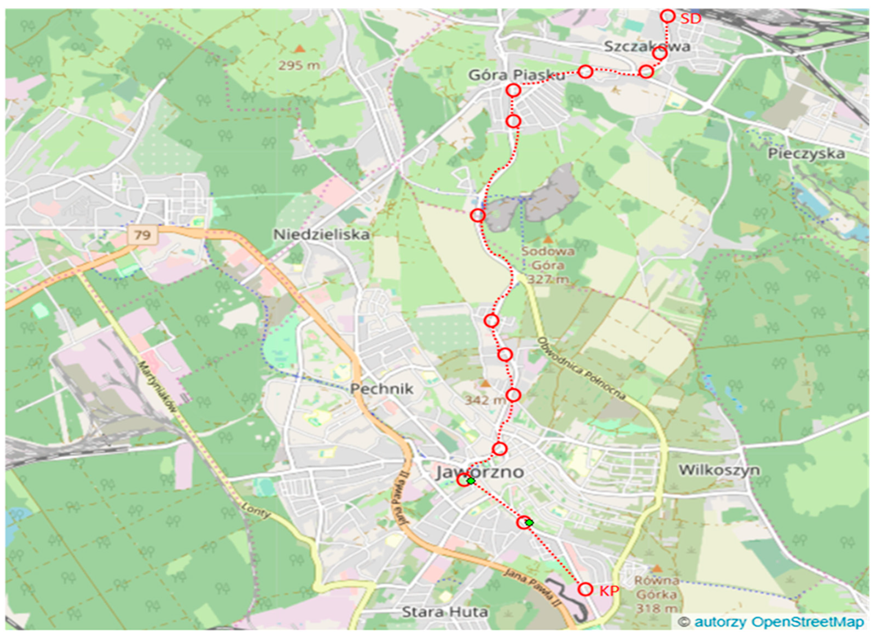
In all, more than 3000 trips between 135 bus stops are available for analysis. Table 1 presents an excerpt from the dataset, which is a list of the raw trip parameters of a bus line with 15 bus stops. The values of energy consumption are derived from the registered levels of bus battery charge. Distances between bus stops and elevation differences are calculated using GPS coordinates and map data. The presented table shows an example of a bus operating on a line in winter: it needs 20 min 12 s and 9.6 kWh of electric energy to cover the route.
A corresponding map is shown in Figure 1, where the red dotted line is the route of the bus line.
2.2. Changes of Energy Demand Due to Weather Conditions
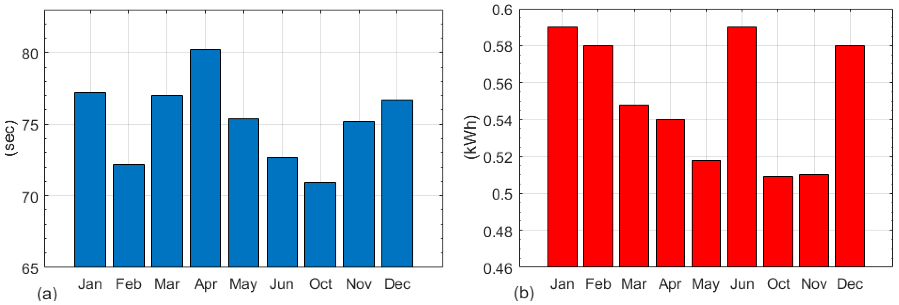
Representative month data are analysed. The demand change follows the increase in travel time in the winter months, but in the summer behaves the other way round. The mean values of energy consumption in January and June is the same and very high, and this accounts for heating in the winter and air-conditioning in the summer, which consume much energy. Figure 2a,b shows the column graphs of the two parameters.
The difference between the highest consumption and lowest amounts to 0.1 kWh, which is 20% of the lowest consumption.
2.3. Changes of Energy Demand Due to Bus Stop Elevation Differences
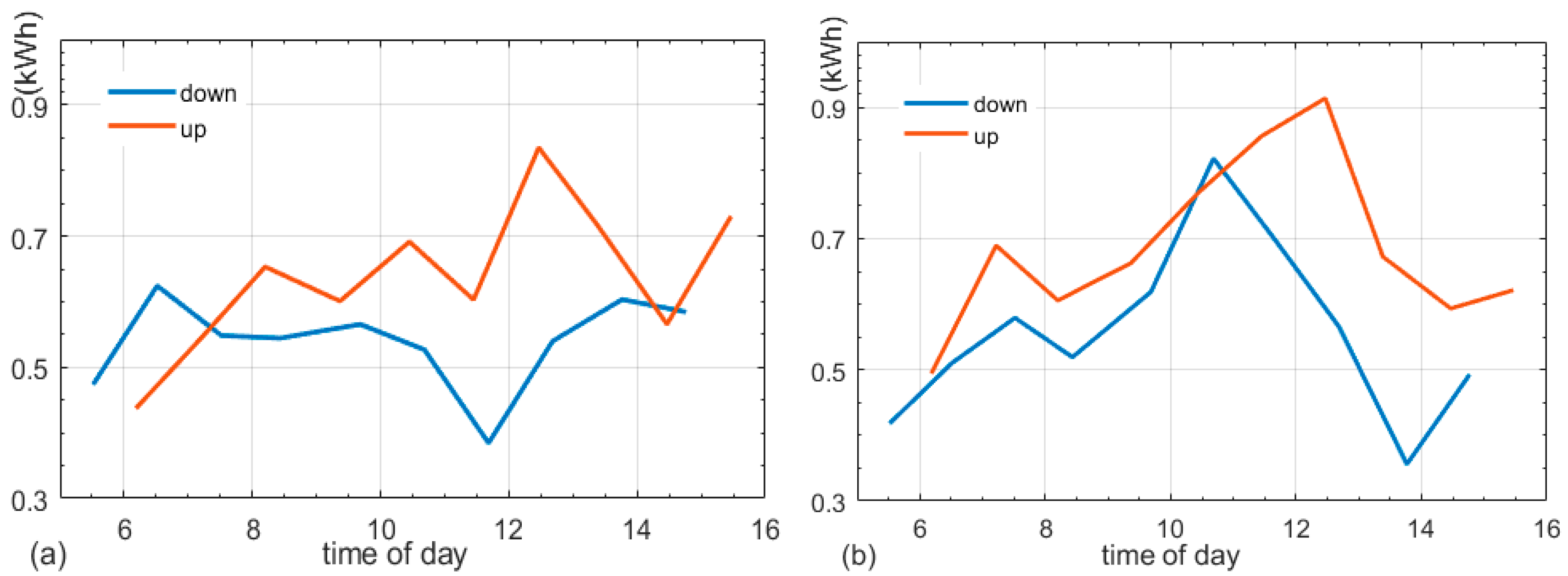
Single trip characteristics are analysed. The movement parameters of the bus trips constitute the input variables of the proposed deep learning network and have a direct impact on the energy expenditure. Significant changes in the energy demand are noted for trips between bus stops at different elevations. One example illustrated in Figure 3a,b shows that a 25 m difference over a 386 m distance brings about an 18% change in December and a 23% change in June.
Interesting is that winter travel has lower energy consumption when travelling downwards in comparison with summer travel. Such dependencies indicate that the factor of elevation change is important for the energy consumption estimation.
The energy consumption also changes during the day of operation. Peaks are observed which can be accounted for a higher number of passengers travelling on the bus. A heavier bus requires more energy to move, but it also takes longer for the passengers to board the bus.
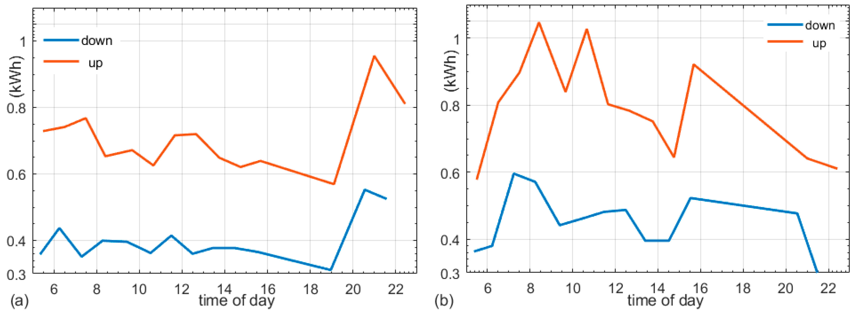
In some cases, the distance between stops can differ when the bus travels upwards and downwards. This happens when the bus lines are routed on one-way roads. Figure 4a,b presents an example of bus trips where the distances in the opposite directions differ significantly: one way it is 592 m, and the other way it is 702 m, with a slight difference in elevations—8 m.
2.4. Energy Consumption Model Variables
The analysis of the relations between the raw bus trip data and the demand for a concise description of the bus trips, which is a prerequisite for the efficient application of a deep learning network (DLN), indicate the necessity to combine some of the collected data. The values of energy consumption change with the trip distance, as the trip travel time changes, when there is adifference in elevation between the stops and when the weather changes. The values of these variables except for weather changes can be derived using the collected trip data. The distance and elevation difference are calculated using the position data of the start and end bus stops of a trip, while trip time is the difference in arrival times at these stops.
The problem of expressing weather conditions is a case of coding non-measurable variables frequently found in applications of neural networks. It is usually solved using some heuristic based on the expertise of the designer of the network.
The weather conditions are strongly related to the time of year and this is the basis for assigning variable values proposed in this study. Table 2 contains the assignment list. The assigned values are a derivative of the energy consumption rates and average monthly weather conditions. Months with similar measured energy consumption rates and weather received the same values. Months with lower consumption rates and better weather had higher values ascribed.
The following variables are used for the description of bus trips:
- —distances between bus stops;
- —travel times: time taken to travel between consecutive bus stops;
- —elevation differences;
- —weather codes.
The energy consumption is expressed using
where n is the number of the bus trip of a bus line.
Table 3 presents the description of the previously (Table 1) quoted bus line using the network input variables.
The bus line data were reported on a winter day w = 2 (February). Travel times mostly exceed 100 s and do not follow the distances between bus stops. The route is hilly, there are 20–24 m changes in elevation. Energy consumption per bus trip is mostly above the 0.8 kWh value.
3. Energy Consumption Model
The energy consumption is modelled using a deep learning network (DLN). This ensures a high level of immunity to corrupted data [26] and a good response to complex relations between the data inputs. These desirable characteristics can be attained in the course of network training using a large dataset of input values, which are derivatives of the collected historical data.
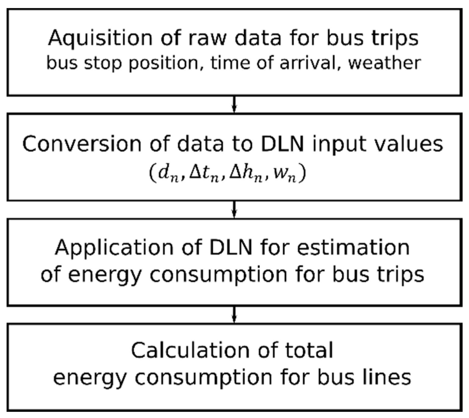
The way of using the model to calculate energy consumption for bus lines is presented in Figure 5. The trained DLN gives estimates of energy consumption for trips between bus stops and requires inputs which are derived from the raw data collected during bus travels.
The first two steps process and prepare the data for the DLN. Different tools for collecting data can be used, for instance, specialised data loggers or mobile devices such as smart phones or smart cameras. The registered trip data are next converted to DLN inputs, and this is done straightforwardly in the case of data loggers and with some effort in the case of smart devices.
The total bus line energy consumption is the sum of estimates for all the bus trips of the line. Additional energy expenditure can be accounted for when the bus waits at the end terminals of the line.
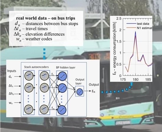
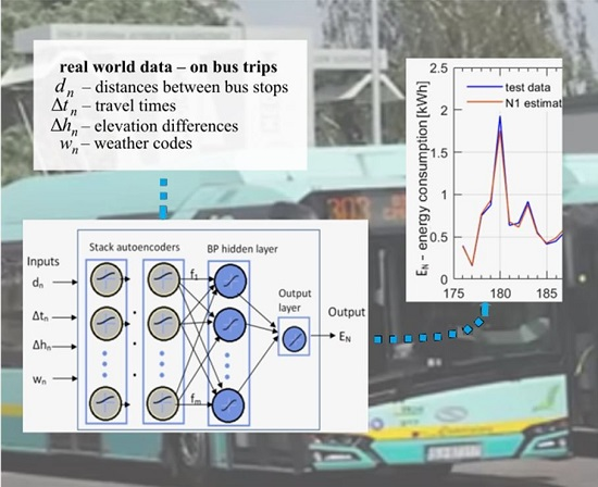
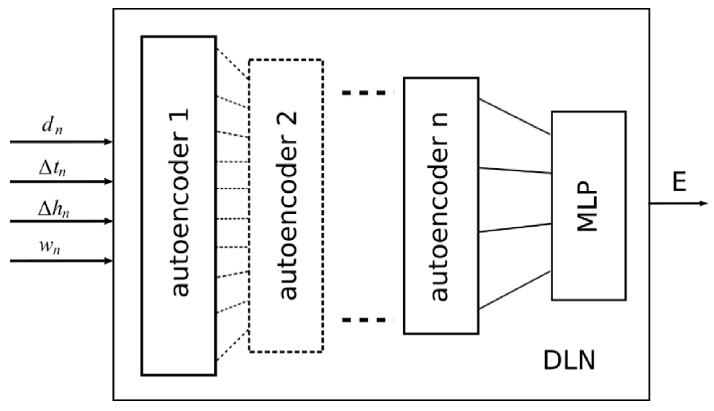
A deep learning network with autoencoders is proposed for modelling the energy consumption function (Equation (1)). Figure 6 shows the draft of the proposed solution.
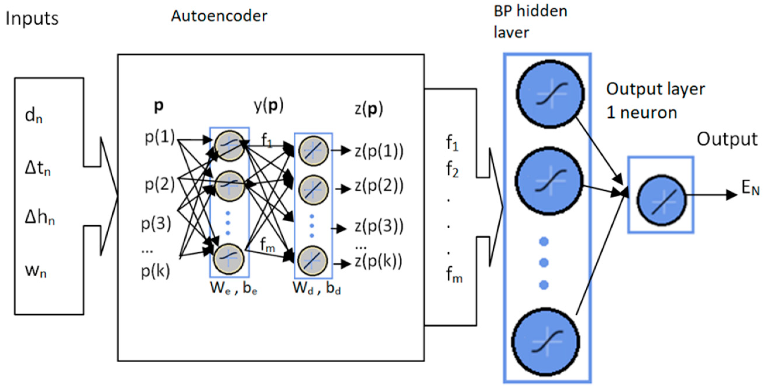
The proposed deep learning network consists of a set of stacked autoencoders, and the outputs of the stack are passed to a multilayer perceptron (MLP). The MLP consists of asingle backpropagation (BP) hidden layer and elaborates the prediction values using the set of features (F) from the last layer of the stack, as presented in Figure 7. The output layer contains one neuron which generates the energy consumption values based on the features elaborated by the last autoencoder of the stack. The hidden layer and the output layer of the DLN are trained using the Levenberg–Marquardt algorithm [28].
The number of neurons in the first autoencoder of the stack is a function of the volatility of the input data. Observed data changes indicate that this behaviour can be represented by several (m) features.
The values of the variables used for the description of bus trips are entered as input values of the DLN. The inputs are . The stack of autoencoders evaluates a set——of features of the input data.
Autoencoders consist of encoders and decoders. An encoder with inputs (p) finds a hidden feature representation of its inputs—y(p).
This set of features constitutes the inputs of the decoder. In the course of the training of the autoencoder, the outputs of the decoder are adjusted to the inputs of the encoder and a set of neuron weights are derived.
where (We,be) and (Wd,bd) are the sets of weight and bias vectors of the encoder and decoder, respectively.
- The neuron activation functions f and g are sigmoidal.
- The goal of the training of the autoencoder is to find weights and bias vectors which give the closest approximation of p using z(p). It is done by minimising the cost function for the k training inputs:
4. Case Study
The model and method are validated using the dataset obtained from the municipal bus company of Jaworzno. Preliminary investigations using a small dataset of bus trips prove that aDLN network with one autoencoder is adequate for modelling energy consumption. The performance of this solution depends on the number of features that are discerned by the autoencoder. There is a distinctive number which in the best way describes the characteristics of the DLN input variables.
Configurations with 10 to 30 neurons in the autoencoder and 6 to 16 neurons in the MLP were tested. The number of MLP neurons is equal to the number of discerned features. The training set consists of 3941 bus trips and the testing set consists of 600 bus trips.
A systematic approach was used to find the required number of neurons of the network. The number of neurons was gradually changed and each new configuration was trained. The maximum number of training epochs for the autoendcoder was set to 1000, and for the MLP layer, 300 epochs. The training was repeated five times and the results of the estimation were evaluated. The set of neuron weights with the best performance was noted.
The errors of estimation are evaluated using the mean absolute percentage error (MAPE) and root mean square error (RMSE):
where E(i) and Er(i) are the estimated and registered energy consumption, respectively, for trip i of the test, n = 600.
The best performing DLN configurations are listed in Table 4.
The DLN (N1) with a 16 neuron autoencoder discerning 16 features, and the MLP consisting of six neurons in the hidden layer, give the lowest MAPE and RMSE errors. The hidden layer elaborates the relations between the feature values and provides data for the output neuron which generates the estimates of energy consumption.
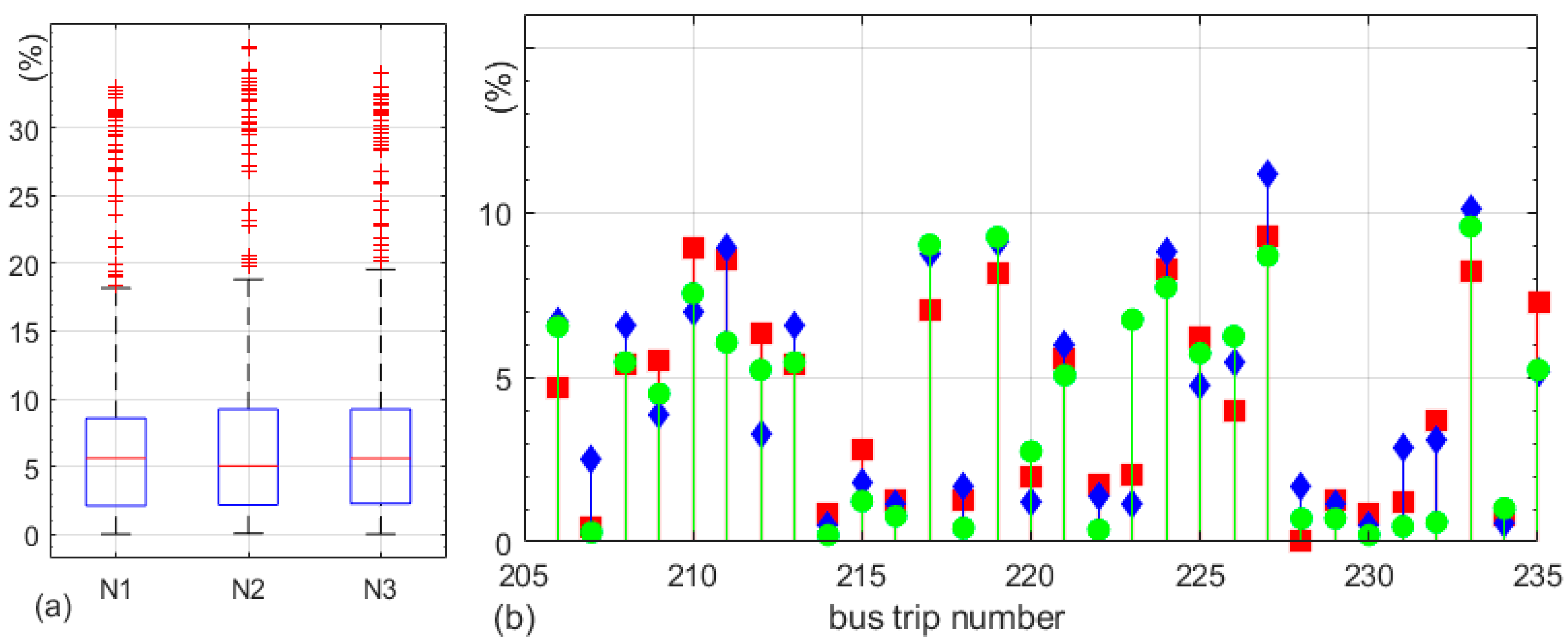
Absolute values of the percentage estimation errors are presented in Figure 8. Figure 8a shows the box plots for the three best networks which present the statistic characteristics of the estimation errors. Error medians for the consecutive networks are 5.6%, 5.0% and 5.6%, the upper adjacent values are 18%, 19% and 20%, and the lower adjacent values are equal to 0. The diverse conditions of the data registration produce a number of outliers which account for about 7% of the test set samples.
Figure 8b presents an excerpt from the set of calculated errors which covers 30 bus trips out of 600. The N1 markers clearly indicate smaller values of errors, while the N3 markers dominate the tops of the stem plots. Error values are scattered, although most of the values fall below the 10% limit. There are no explicit relations between the N1, N2 and N3 estimation errors.
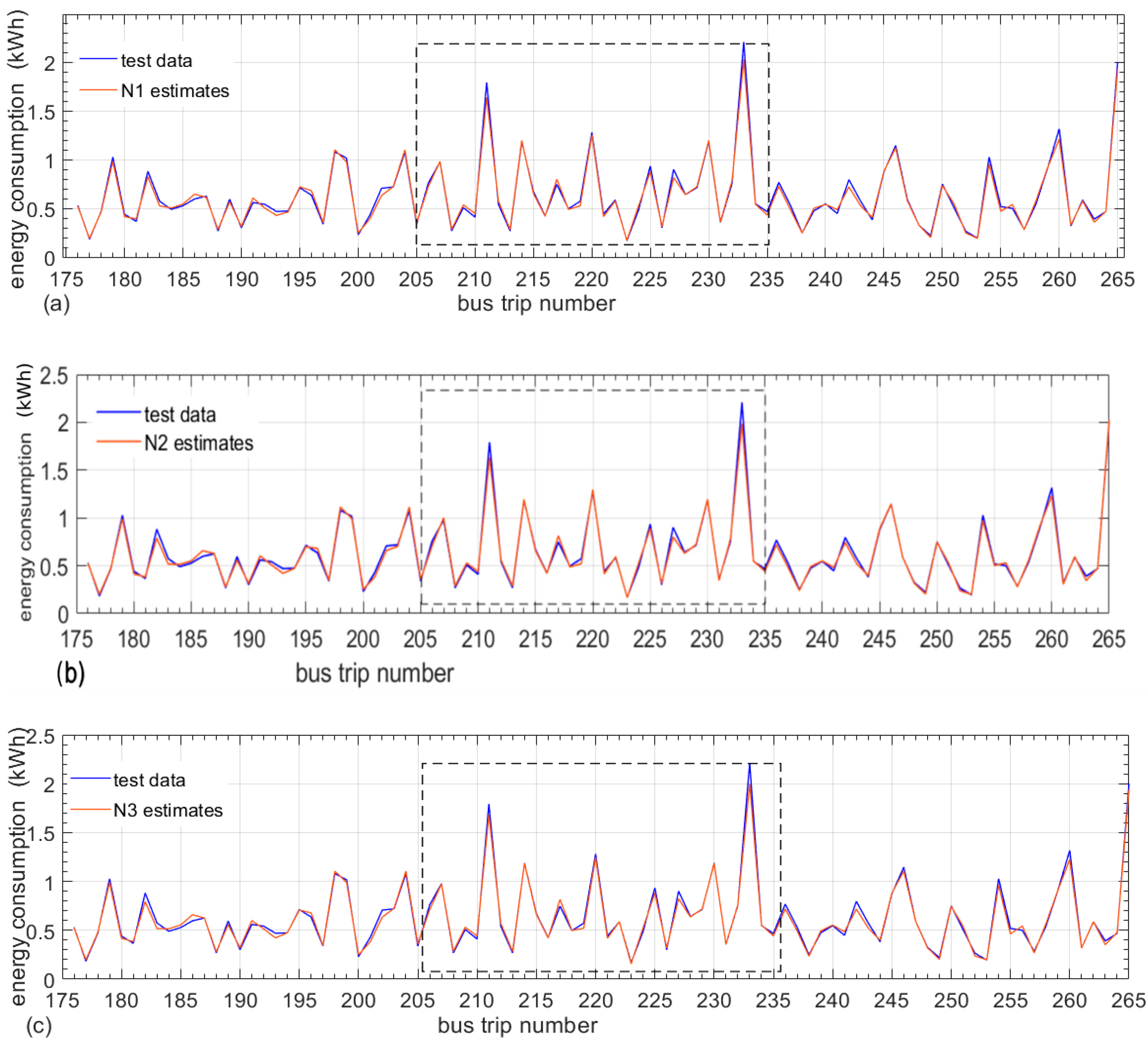
Figure 9 presents the estimation performance for a larger excerpt of test data amounting to 90 bus trips. The test data and estimates graphs are paired for comparison. Rectangles cover the range of bus trips which are depicted in Figure 8b. The graphs confirm a mixed performance of the networks. There are samples correctly mapped which have large and small values.
Graphs in Figure 9 differ slightly, on par with the statistics. Careful analysis unravels more overlapped lines in Figure 9a, which suggest a better fit of the estimates to the test data. The characteristics of the whole set of test and estimated data confirm the best performance of the N1 network.
Comparison with a Multiple Linear Regression (MLR) Model of Bus Trip Data
The course of development of the DLNs shows that the relations between input variables do not exhibit extraordinary behaviour. This observation suggests that a multiple linear regression model could satisfy the requirements of the energy consumption estimation. The multiple regression model is based on the assumptions that there is a linear relationship between the variables and the variables are not too highly correlated with each other. The multiple regression (MLR) model uses several explanatory variables to predict the outcome of a response variable. In this case, the network input variables are the explanatory variables and the estimated energy consumption (En) is the response as in Equation (6):
A stochastic gradient descent is used to solve the problem of finding the coefficients (m) of the equation. The same set as in the case of DLN training of the bus trip data is processed. Results prove that the proposed model is suitable to estimate energy consumption. The coefficient of determination (R2) reached the value 0.89. The standard errors of the coefficients m4−m1 are {0.101, 3.144, 0.016, −0.123}, and these show that all of the explanatory variables are necessary for the calculation of the estimates.
The errors of estimation reached the values MAPE = 8.2% and RMSE = 0.085.
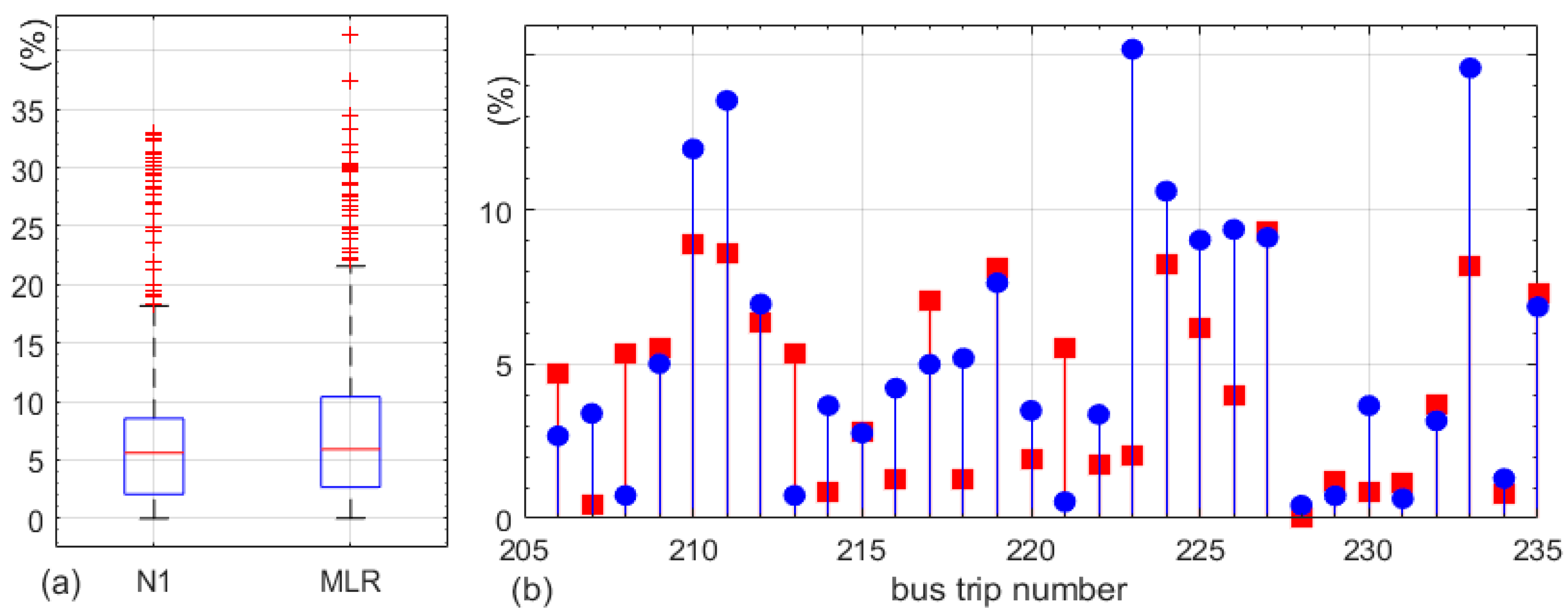
The box plots in Figure 10a illustrate the comparison of the statistic characteristics of the estimation errors of the best network, N1, and the MLR model. Error medians for N1 and the MLR model are 5.6% and 5.9%, the upper adjacent values are 18% and 22%, and the lower adjacent values are equal to 0. The MLR model gives asimilar number of outliers that is about 7% of the test samples. The characteristics confirm a better performance of the N1 network, especially the lower value of the upper adjacent and the smaller value of 75%.
Figure 10b puts together the N1 and MLR errors for comparison. Most of the MLR model markers stay above N1, clearly showing that the MLR model gives larger estimation errors.
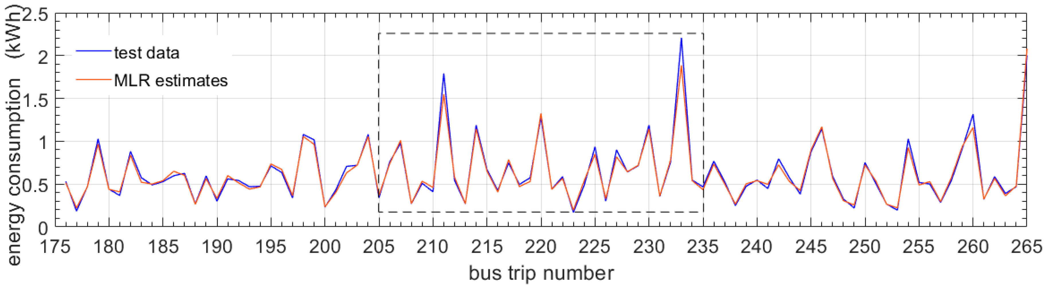
Figure 11 presents the estimation performance, and again, the test data and estimates graphs are paired for comparison. The rectangle covers the range of bus trips which are depicted in Figure 10b. The graphs confirm a mixed performance of the MLR model. The discrepancies between graphs are larger than in the case of the N1 DLN.
5. Discussion
The proposed model and method of estimation of energy consumption meet the expected requirements for a robust and efficient tool. The application of the trained DLN enables an accurate and fast calculation of the energy needs for bus trips as well as for whole bus lines operated by battery electric vehicles. The number of variables representing energy consumption is reduced to parameters of bus trips between bus stops. The values of these variables can be recorded on a daily basis and used for updating the model. A larger database will be useful for extending the training sets and achieving lower estimation errors.
The proposed approach gives an acceptable error for practical use. Collected real-world data on bus operations show that factory specifications of bus powertrains and especially of battery performance are over-estimated in many cases by tens of percents.
The references do not explicitly present the error rates of the proposed models. Indirect comments hint on errors in the range of a few percent but there are many restrictions on the use of the models in real-world conditions.
The proposed energy consumption model based on DLN is more accurate than an MLR-based model. The difference is not substantial, however, the trained DLN is resistant to inputs of corrupted data, whereas the MLR model responds with high errors. DLN generates a response based on the latest training data. Lack of some input data is corrected by the network and the response does not suffer greatly [26]. This property contributes to the robustness of the proposed DLN-based energy consumption model.
6. Conclusions
Estimation results are used for the energy analysis of bus lines. The resolution of analysis, bus stop to bus stop, is adequate for locating energy deficient places of the bus network. The positions of bus stops are mostly determined by transport needs of the inhabitants. Energy deficient nodes are potential locations of charging stations. Bus companies can adjust bus schedules to evade the energy bottlenecks of network.
Knowledge of energy consumption in the bus network is beneficial for the planning of the expansion of the bus fleet, modernising of the infrastructure and management of the daily operations. A large number of energy deficient places pose a question whether is it more advantageous to build charging stations or buy buses with batteries of higher capacity.
The designed DLN for the estimation of energy consumption performs satisfactorily in the case of ahomogenous fleet of battery electric vehicles. Currently, new companies enter the electric bus market, and so there is a need to include the fleet variability in the estimation model and this is the future study problem.
Author Contributions
Conceptualization, T.P.; methodology, T.P.; software, T.P.; validation, T.P.; formal analysis, T.P.; investigation, T.P. and W.P.; resources, T.P.; data curation, T.P.; writing—original draft preparation, T.P.; writing—review and editing, W.P.; visualization, W.P.; supervision, T.P. and W.P.; project administration, T.P.; funding acquisition, T.P. All authors have read and agreed to the published version of the manuscript.
Funding
Publication supported as a part of the Rector’s grant in the area of scientific research and development works. Silesian University of Technology, grant number 12/050/RGJ19/0075.
Acknowledgments
The authors wish to thank PKM Jaworzno for providing data used for these studies.
Conflicts of Interest
The authors declare no conflict of interest. The funders had no role in the design of the study; in the collection, analyses, or interpretation of data; in the writing of the manuscript, or in the decision to publish the results.
References
- Bloomberg New Energy Finance report. Electric Buses in Cities: Driving towards Cleaner Air and Lower CO2; Bloomberg New Energy Finance Report: New York, NY, USA, 2018. [Google Scholar]
- Hooftman, N.; Messagie, M.; Coosemans, T. Analysis of the Potential for Electric Buses, a Study Accomplished for the European Copper Institute; 2019; pp. 1–18. Available online: https://leonardo-energy.pl/wp-content/uploads/2019/02/Analysis-of-the-potential-for-electric-buses.pdf (accessed on 20 January 2020).
- UITP (Union Internationale des Transports Publics). Statistics Brief Global Bus Survey (003).pdf. 2019. Available online: https://www.uitp.org/sites/default/files/cck-focus-papers-files/Statistics%20Brief_Global%20bus%20survey%20%28003%29.pdf (accessed on 20 January 2020).
- European Commission. White Paper: Roadmap to a Single European Transport Area—Towards a Competitive and Resource Efficient Transport System; COM (2011) 144 final; European Commission: Brussels, Belgium, 2011; pp. 1–31. [Google Scholar]
- Tsiropoulos, I.; Tarvydas., D.; Lebedeva, N. Li-ion batteries for mobility and stationary storage applications. In Scenarios for Costs and Market Growth; Publications Office of the European Union: Luxembourg, 2018. [Google Scholar] [CrossRef]
- Mathieu, L. Electric Buses Arrive on Time. Marketplace, Economic, Technology, Environmental and Policy Perspectives for Fully Electric Buses in the EU. Transport and Environment. 2018. Available online: https://www.transportenvironment.org/sites/te/files/publications/Electric%20buses%20arrive%20on%20time.pdf (accessed on 20 January 2020).
- Clairand, J.-M.; Guerra-Terán, P.; Serrano-Guerrero, X.; González-Rodríguez, M.; Escrivá-Escrivá, G. Electric Vehicles for Public Transportation in Power Systems: A Review of Methodologies. Energies 2019, 12, 3114. [Google Scholar] [CrossRef] [Green Version]
- Kivekäs, K.; Lajunen, A.; Vepsäläinen, J.; Tammi, K. City Bus Powertrain Comparison: Driving Cycle Variation and Passenger Load Sensitivity Analysis. Energies 2018, 11, 1755. [Google Scholar] [CrossRef] [Green Version]
- Vepsäläinen, J.; Ritari, A.; Lajunen, A.; Kivekäs, K.; Tammi, K. Energy Uncertainty Analysis of Electric Buses. Energies 2018, 11, 3267. [Google Scholar] [CrossRef] [Green Version]
- Paul, T.; Yamada, H. Operation and charging scheduling of electric buses in a city bus route network. In Proceedings of the IEEE 17th International Conference on Intelligent Transportation Systems (ITSC), Qingdao, China, 8–11 October 2014; pp. 2780–2786. [Google Scholar] [CrossRef]
- Wang, Y.; Huang, Y.; Xu, J.; Barclay, N. Optimal recharging scheduling for urban electric buses: A case study in Davis. Transp. Res. Part E Logis Transp. Rev. 2017, 115–132. [Google Scholar] [CrossRef]
- Xylia, M.; Leduc, S.; Patrizio, P.; Kraxner, F.; Silveira, S. Locating charging infrastructure for electric buses in Stockholm. Transp. Res. Part C Emerg. Technol. 2017, 78, 183–200. [Google Scholar] [CrossRef]
- Vepsäläinen, J.; Otto, K.; Lajunen, A.; Tammi, K. Computationally efficient model for energy demand prediction of electric city bus in varying operating conditions. Energy 2019, 169, 433–443. [Google Scholar] [CrossRef]
- Vepsäläinen, J.; Kivekäs, K.; Otto, K.; Lajunen, A.; Tammi, K. Development and validation of energy demand uncertainty model for electric city buses. Transp. Res. Part D Transp. Environ. 2018, 63, 347–361. [Google Scholar] [CrossRef]
- Gao, Y.; Guo, S.; Ren, J.; Zhao, Z.; Ehsan, A.; Zheng, Y. An Electric Bus Power Consumption Model and Optimization of Charging Scheduling Concerning Multi-External Factors. Energies 2018, 11, 2060. [Google Scholar] [CrossRef] [Green Version]
- Beckers, C.J.J.; Besselink, I.J.M.; Frints, J.J.M.; Nijmeijer, H. Energy Consumption Prediction for Electric City Buses. In Proceedings of the 13th ITS European Congress, Brainport, The Netherlands, 3–6 June 2019; Available online: https://www.researchgate.net/publication/335542182_Energy_Consumption_Prediction_for_Electric_City_Buses (accessed on 20 January 2020).
- Wang, J.; Besselink, I.J.M.; Nijmeijer, H. Battery electric vehicle energy consumption modelling for range estimation. Int. J. Electr. Hybrid Veh. 2017, 9, 79–102. [Google Scholar] [CrossRef]
- Sarrafan, K.; Sutanto, D.; Muttaqi, K.M.; Town, G. Accurate range estimation for an electric vehicle including changing environmental conditions and traction system efficiency. IET Electr. Syst. Transp. 2017, 7, 117–124. [Google Scholar] [CrossRef] [Green Version]
- De Filippo, G.; Marano, V.; Sioshansi, R. Simulation of an electric transportation system at The Ohio State University. Appl. Energy 2014, 113, 1686–1691. [Google Scholar] [CrossRef]
- Vilppo, O.; Markkula, J. Feasibility of electric buses in public transport. World Electr. Veh. J. 2015, 7, 357–365. [Google Scholar] [CrossRef] [Green Version]
- Sinhuber, P.; Rohlfs, W.; Sauer, D.U. Study on power and energy demand for sizing the energy storage systems for electrified local public transport buses. In Proceedings of the IEEE Vehicle Power and Propulsion Conference, Seoul, Korea, 9–12 October 2012; pp. 315–320. [Google Scholar] [CrossRef]
- Galleta, M.; Massiera, T.; Hamacherb, T. Estimation of the energy demand of electric buses based on real-world data for large-scale public transport networks. Appl. Energy 2018, 230, 344–356. [Google Scholar] [CrossRef]
- De Cauwer, C.; Van Mierlo, J.; Coosemans, T. Energy Consumption Prediction for Electric Vehicles Based on Real-World Data. Energies 2015, 8, 8573–8593. [Google Scholar] [CrossRef]
- Kanarachos, S.; Mathew, J.; Fitzpatrick, M.E. Instantaneous vehicle fuel consumption estimation using smartphones and recurrent neural networks. Expert Syst. Appl. 2019, 120, 436–447. [Google Scholar] [CrossRef]
- Lin, C.; Zhou, X.; Wu, D.; Gong, B. Estimation of Emissions at Signalized Intersections Using an Improved MOVES Model with GPS Data. Int. J. Environ. Res. Public Health 2019, 16, 3647. [Google Scholar] [CrossRef] [PubMed] [Green Version]
- Ping, P.; Qin, W.; Xu, Y.; Miyajima, C.; Takeda, K. Impact of Driver Behavior on Fuel Consumption: Classification, Evaluation and Prediction Using Machine Learning. IEEE Access 2019, 7, 78515–78532. [Google Scholar] [CrossRef]
- Pamuła, T. Impact of data loss for prediction of traffic flow on an urban road using neural networks. IEEE Trans. Intell. Transp. Syst. 2019, 20, 1000–1009. [Google Scholar] [CrossRef]
- Marquard, D. An algorithm for least-squares estimation of nonlinear parameters, SIAMJ. Appl. Math. 1963, 11, 431–441. [Google Scholar] [CrossRef]
- Bottou, L. Online Algorithms and Stochastic Approximations. In On-Line Learning in Neural Networks; Saad, D., Ed.; Cambridge University Press: Cambridge, UK, 1999; pp. 9–42. [Google Scholar] [CrossRef] [Green Version]
Figure 1.
Route of an analysed bus line.

Figure 2.
(a) Mean travel time, (b) mean energy consumption per bus trip.

Figure 3.
Mean energy consumption for upward and downward bus trips during a day in (a) winter and (b) summer.
Figure 3.
Mean energy consumption for upward and downward bus trips during a day in (a) winter and (b) summer.

Figure 4.
Mean energy consumption for upward and downward bus trips with a small elevation difference but longer upward distance in (a) winter and (b) summer.
Figure 4.
Mean energy consumption for upward and downward bus trips with a small elevation difference but longer upward distance in (a) winter and (b) summer.

Figure 5.
Block diagram of the estimation method.

Figure 6.
Energy consumption estimation model using a deep learning network.

Figure 7.
Autoencoder stack and multilayer perceptron (MLP) of the energy consumption estimation DLN.
Figure 7.
Autoencoder stack and multilayer perceptron (MLP) of the energy consumption estimation DLN.

Figure 8.
Absolute value of estimation errors for networks N1, N2, N3: (a) box plots and (b) stem plots of an example range of bus trips used in the testing.
Figure 8.
Absolute value of estimation errors for networks N1, N2, N3: (a) box plots and (b) stem plots of an example range of bus trips used in the testing.

Figure 9.
Test data and estimated values using the DLN: (a) N1, (b) N2 and(c) N3.

Figure 10.
Absolute value of estimation errors for best network and regression model: (a) box plots and (b) stem plot of an example range of bus trips used in testing.
Figure 10.
Absolute value of estimation errors for best network and regression model: (a) box plots and (b) stem plot of an example range of bus trips used in testing.

Figure 11.
Test data and estimated values using the multiple regression (MLR) model.


Table 1.
Parameters of bus trips for a 15-stop bus line.
| No | Bus Stop Name | Longitude | Latitude | Time of Arrival | Energy Consumption (kWh) |
|---|---|---|---|---|---|
| 1 | KP | 19.284000 | 50.193042 | 05:06:09 | - |
| 2 | Ro | 19.279483 | 50.197584 | 05:07:34 | 0.67 |
| 3 | UM | 19.27655 | 50.199220 | 05:08:34 | 0.48 |
| 4 | Ce | 19.271324 | 50.203323 | 05:10:29 | 0.91 |
| 5 | Ry | 19.275168 | 50.204289 | 05:12:15 | 0.84 |
| 6 | WW | 19.275488 | 50.210060 | 05:14:00 | 0.83 |
| 7 | WG | 19.275142 | 50.214693 | 05:15:05 | 0.51 |
| 8 | Wa | 19.274221 | 50.218299 | 05:16:50 | 0.83 |
| 9 | Ge | 19.271800 | 50.227215 | 05:19:31 | 1.28 |
| 10 | GPK | 19.275809 | 50.235738 | 05:21:21 | 0.87 |
| 11 | GP | 19.277024 | 50.239224 | 05:22:56 | 0.75 |
| 12 | SP | 19.285006 | 50.240703 | 05:24:01 | 0.51 |
| 13 | SOG | 19.289323 | 50.240417 | 05:24:26 | 0.20 |
| 14 | SP | 19.294436 | 50.243652 | 05:25:51 | 0.67 |
| 15 | SD | 19.292681 | 50.246734 | 05:26:21 | 0.24 |
Table 2.
Weather conditions coding values.
| January | February | March | April | May | June | October | November | December |
|---|---|---|---|---|---|---|---|---|
| 1 | 2 | 3 | 3 | 4 | 1 | 4 | 4 | 2 |
Table 3.
Values of the deep learning network (DLN) inputs.
| No | Bus Stop Name | Trip Time (s) | Trip Distance (m) | Change of Elevation (m) | Weather Conditions | Energy Consumption (kWh) |
|---|---|---|---|---|---|---|
| 1 | KP | - | - | - | - | - |
| 2 | Ro | 85 | 599 | 12 | 2 | 0.67 |
| 3 | UM | 60 | 277 | 6 | 2 | 0.48 |
| 4 | Ce | 115 | 589 | −7 | 2 | 0.91 |
| 5 | Ry | 106 | 294 | 17 | 2 | 0.84 |
| 6 | WW | 105 | 643 | 20 | 2 | 0.83 |
| 7 | WG | 65 | 516 | −12 | 2 | 0.51 |
| 8 | Wa | 105 | 407 | −3 | 2 | 0.83 |
| 9 | Ge | 161 | 1007 | −24 | 2 | 1.28 |
| 10 | GPK | 110 | 991 | 14 | 2 | 0.87 |
| 11 | GP | 95 | 398 | 2 | 2 | 0.75 |
| 12 | SP | 65 | 592 | −8 | 2 | 0.51 |
| 13 | SOG | 25 | 309 | −8 | 2 | 0.20 |
| 14 | SP | 85 | 512 | −22 | 2 | 0.67 |
| 15 | SD | 30 | 365 | −1 | 2 | 0.24 |
Table 4.
Estimation errors for the different DLN configurations.
| Network | DLN Configuration | MAPE (%) | RMSE |
|---|---|---|---|
| N1 | 4-16a-6-1 | 7.1 | 0.077 |
| N2 | 4-12a-16-1 | 7.2 | 0.080 |
| N3 | 4-20a-16-1 | 7.3 | 0.081 |
© 2020 by the authors. Licensee MDPI, Basel, Switzerland. This article is an open access article distributed under the terms and conditions of the Creative Commons Attribution (CC BY) license (http://creativecommons.org/licenses/by/4.0/).
Share and Cite
MDPI and ACS Style
Pamuła, T.; Pamuła, W. Estimation of the Energy Consumption of Battery Electric Buses for Public Transport Networks Using Real-World Data and Deep Learning. Energies 2020, 13, 2340. https://doi.org/10.3390/en13092340
AMA Style
Pamuła T, Pamuła W. Estimation of the Energy Consumption of Battery Electric Buses for Public Transport Networks Using Real-World Data and Deep Learning. Energies. 2020; 13(9):2340. https://doi.org/10.3390/en13092340
Chicago/Turabian StylePamuła, Teresa, and Wiesław Pamuła. 2020. "Estimation of the Energy Consumption of Battery Electric Buses for Public Transport Networks Using Real-World Data and Deep Learning" Energies 13, no. 9: 2340. https://doi.org/10.3390/en13092340
Note that from the first issue of 2016, this journal uses article numbers instead of page numbers. See further details here.