Article

Maritime Transport in a Life Cycle Perspective: How Fuels, Vessel Types, and Operational Profiles Influence Energy Demand and Greenhouse Gas Emissions

by
Grusche J. Seithe
1,
Alexandra Bonou
2,
Dimitrios Giannopoulos
2,
Chariklia A. Georgopoulou
3 and
Maria Founti
2,*
1
DNV-GL Group Technology and Research, Maritime Transport, Veritasveien 1, 1363 Høvik, Norway
2
Laboratory Of Heterogeneous Mixtures and Combustion Systems, School of Mechanical Engineering, National Technical University of Athens, Polytechnioupoli-Zografou Heroon Polytechniou 9, 15780 Athens, Greece
3
DNV-GL Maritime R&D and Advisory, South East Europe and Middle East, 5 Aitolikou Str., 18545 Piraeus, Greece
*
Author to whom correspondence should be addressed.
Energies 2020, 13(11), 2739; https://doi.org/10.3390/en13112739
Submission received: 28 April 2020 / Revised: 21 May 2020 / Accepted: 21 May 2020 / Published: 29 May 2020

Abstract

:
A “Well-to-Propeller” Life Cycle Assessment of maritime transport was performed with a European geographical focus. Four typical types of vessels with specific operational profiles were assessed: a container vessel and a tanker (both with 2-stroke engines), a passenger roll-on/roll-off (Ro-Pax) and a cruise vessel (both with 4-stroke engines). All main engines were dual fuel operated with Heavy Fuel Oil (HFO) or Liquefied Natural Gas (LNG). Alternative onshore and offshore fuel supply chains were considered. Primary energy use and greenhouse gas emissions were assessed. Raw material extraction was found to be the most impactful life cycle stage (~90% of total energy use). Regarding greenhouse gases, liquefaction was the key issue. When transitioning from HFO to LNG, the systems were mainly influenced by a reduction in cargo capacity due to bunkering requirements and methane slip, which depends on the fuel supply chain (onshore has 64% more slip than offshore) and the engine type (4-stroke engines have 20% more slip than 2-stroke engines). The combination of alternative fuel supply chains and specific operational profiles allowed for a complete system assessment. The results demonstrated that multiple opposing drivers affect the environmental performance of maritime transport, a useful insight towards establishing emission abatement strategies.

Graphical Abstract

1. Introduction

Maritime transport is relatively clean compared to its road and air counterparts [1,2,3]. Yet, the sector is a significant contributor to local pollution inventories given that its emissions are mainly (>70%) deposited within 400 km of land, resulting in environmental and human health impacts [4,5,6]. Beyond the contribution at a local scale, maritime transport is also a notable contributor to global impacts, such as climate change, accounting for 2.5% of the global Greenhouse Gas (GHG) budget, and emissions are expected to increase by 50–250% by 2050 due to a rapid increase in the demand for transport [7,8].
Hence, while maintaining the sector’s continuous growth [9] there is a need for lowering the corresponding environmental impacts. In this context, the International Maritime Organization (IMO) through its Convention of Prevention of Pollution from Ships (MARPOL 73/78), has set limits for SOx and NOx emissions globally and applies even stricter regulations within designated Emission Control Areas (ECAs) [10,11]. As a response, researchers have looked into emission reduction potentials. Indeed, the present research was part of the EU funded project ECCO-MATE— Experimental and Computational Tools for Combustion Optimization in Marine and Automotive Engines [12].
Contrary to the well-established limitations for NOx and SOx, the GHG reduction requirements are less firm in the maritime transport sector. IMO suggests shipping companies employ the Energy Efficiency Operational Indicator (EEOI) as a CO2 monitoring tool [13]. However, EEOI is of limited scope since it only accounts for on-board combustion, disregarding upstream emissions from production and distribution. Additionally, it only monitors CO2, instead of all the GHGs defined by the Intergovernmental Panel for Climate Change (IPCC) [14], which might lead to a distorted view concerning the effectiveness of environmental strategies for emission abatement. This calls for more comprehensive environmental assessment frameworks such as the one provided by Life Cycle Assessment (LCA).
LCA is a state of the art, well-established, and ISO standardized methodology which allows us to take into account the emission of several pollutants across the life cycle of a product or system from raw material extraction to final disposal [15]. LCA is used across economic sectors, e.g., for establishing environmental performance indicators and labels [16]. Focusing at the energy sector, LCA provides a solid ground for ecodesign, e.g., of wind energy systems [17], and for optimizing new innovations, e.g., Power to Gas systems [18].
Juxtaposing EEOI with LCA-based indicators seems particularly relevant for the case where Liquefied Natural Gas (LNG) is introduced as a replacement for Heavy Fuel Oil (HFO). This commonly adopted emission abatement strategy [19,20,21] has on the one hand several advantages such as the simultaneous reduction of SOx, NOx, and GHG [22,23]; its compliance to ECAs regulations; its economic advantage compared to other low sulphur fuels; and its technology readiness in the market [24,25,26]. On the other hand though, LNG is associated with methane leakages during upstream processes [27]. Provided that the Global Warming Potential (GWP) of methane is 25 times higher than that of CO2 [28], such occurrences should not be underestimated [23,29].
Looking at relevant literature, there is indeed a number of LCA studies focusing on marine fuels and acknowledging the value of LCA as a complementary utility to regulatory measures [30,31,32]. Most studies focus on fuel supply chain comparisons, e.g., between residual oil, conventional diesel, low sulphur diesel, compressed natural gas, heavy fuel oil, marine gas-to-liquid fuel, and biofuels, while novel multicriteria analysis methods are introduced for more comprehensive comparisons [23,33,34,35].
Little focus is put on the operations at sea. Literature studies on maritime LCAs, even recent ones [36], rarely account for realistic operational modes and they typically consider generic standard shiploads. This crude assumption may be necessary due to data unavailability and variability between regions; it is, however, far from being representative of real-life conditions, and it imposes limitations in terms of the representativeness of LCA results. Some literature studies do address this gap. Mountaneas et al., (2015) presents a framework for LCA taking into account all stages of the ship lifecycle; however, no evaluation of the effect of the fuel supply chain is considered or of the impact of different fuel types [37]. In a more complete study, Thomson et al., (2015) evaluated the GHG reduction potential when transitioning to natural gas with a focus on the United States [25].
With this background, the present study focuses on Europe and performs a maritime transport LCA that couples the supply chain of conventional and prospective marine fuels with realistic operational profiles for various types of vessels operated via dual fuel engines. The objective of the assessment is to showcase the importance of accounting all the life cycle stages and specific conditions from well to propeller in maritime transport LCAs and the advantage of LCA-derived environmental performance indicators. This work responds to a research need for holistic approaches and multi-objective decision support to enhance environmental sustainability in maritime shipping and the transport sector in general [38,39,40,41].

2. Materials and Methods

Taking a life cycle perspective, the maritime transport system can be split into the “Well-to-Tank” (upstream) and “Tank-to-Propeller” (downstream) parts. The former includes the raw material extraction process, the transport to the refinery or liquefaction plant, the refinery or liquefaction process, and the distribution to the bunker station inside the port. The latter includes the combustion on board different vessels.
“Well-to-Propeller” LCAs of heavy fuel oil (HFO) (as the reference) and Liquefied Natural Gas (LNG) (as the close-future perspective marine fuel) were performed following the International Reference Life Cycle Data System (ILCD) Handbook for LCA [42]. The goal of the LCAs and the intended applications coincide with the aforementioned research objectives. Four types of vessels were considered, i.e., a container vessel, a tanker, a passenger roll-on/roll-off (Ro-Pax) vessel, and a cruise vessel, equipped either with two-stroke or four-stroke engines (Figure 1). The functional unit (FU), which reflects the primary function of the system (i.e., the transport work of the vessel), was defined as “1 t of cargo transported for 1 km (1 tkm)” for all investigated vessels except of the cruise vessel for which the functional unit was set as “1 passenger transported for 1 km (1 pkm)”. The geographical boundaries of the study were in Europe.
Since this was a descriptive study aiming to document the analysed system, the modelling principle for the life cycle inventory followed an attributional LCA approach where the inventory included input and output flows of all processes as they occur, e.g., along existing supply chains [42]. The detailed investigation of fuel markets and the long-term consequences of shifting towards cleaner fuels were out of scope. The generic database ecoinvent v2.2 [43] was used for modelling the background data (infrastructure, energy, and transport technologies) in the Life Cycle Inventory. The impact categories to focus on were climate change, measured in CO2-eq, and Primary Energy Use (PEU), measured in MJ. For the impact assessment, characterisation factors for the potential contribution to climate change were based on IPCC findings on a 100-year perspective [14]. The life cycle of the systems was modelled in SimaPro v7 software [44].

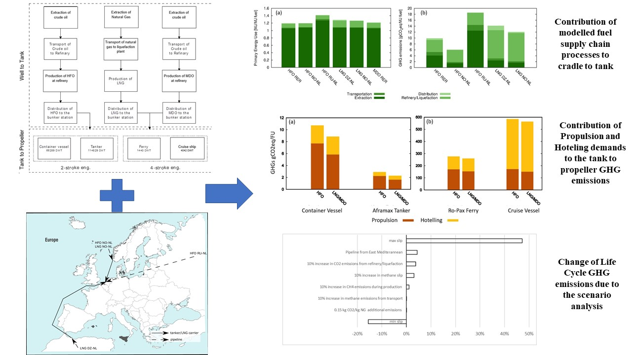
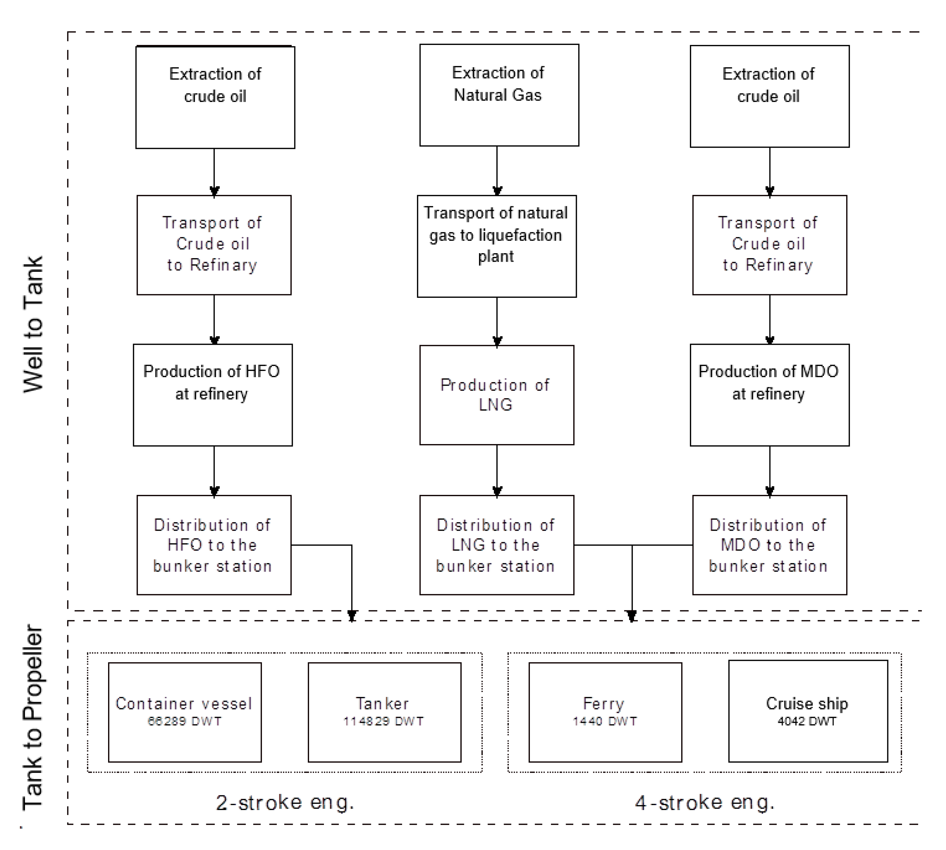
2.1. System Description: Vessel, Engine and Fuel Types

To ensure realistic system description and boundary completeness, the technical characteristics in terms of fuel types, vessel types and propulsion engines were defined. The selected combination of engines and vessel types, shown in Table 1, corresponds to typical maritime transport conditions, provided by DNV GL, industrial partner of the ECCO-MATE research project. The propulsion Main Engines (ME) are Dual Fuel (DF) (either HFO or LNG). The Auxiliary Engines (AE) are used to cover hoteling demands. The fuel selection is representative of current fuel consumption for the marine sector: HFO accounts for 84% of the total fuel consumption in the sector, while for LNG, the share reaches 16% [45]. An additional input of Marine Diesel Oil (MDO) has been considered as the pilot fuel for the DF engines in gas mode and as the fuel for the AEs. The properties of the investigated fuels, as used in this study, are given in Table 2. The type of engine and the type of fuel affect the overall system performance; specifically:
  • The engine characteristics affect the methane slip. Two-stroke engines use high-pressure gas-injection technology that reduces the methane slip to less than 0.1% [46]. The methane slip for the four-stroke engines in gas mode is considered 2% for high and 3% for low loads [46].
  • The fuel type affects the cargo capacity. The higher bunker storage requirement for LNG decreases the cargo capacity for the container vessel and the ferry by 1.8% and 4%, respectively [23,47]. In the case of the tanker and the cruise vessel, the cargo/passenger capacity is not affected by the choice of fuel. For the former, the LNG is stored in an external tank transported on the deck of the vessel [48], while for the latter it is assumed that in new vessels the space loss is counterbalanced by a reduction in space requirements of facilities such as cabins.

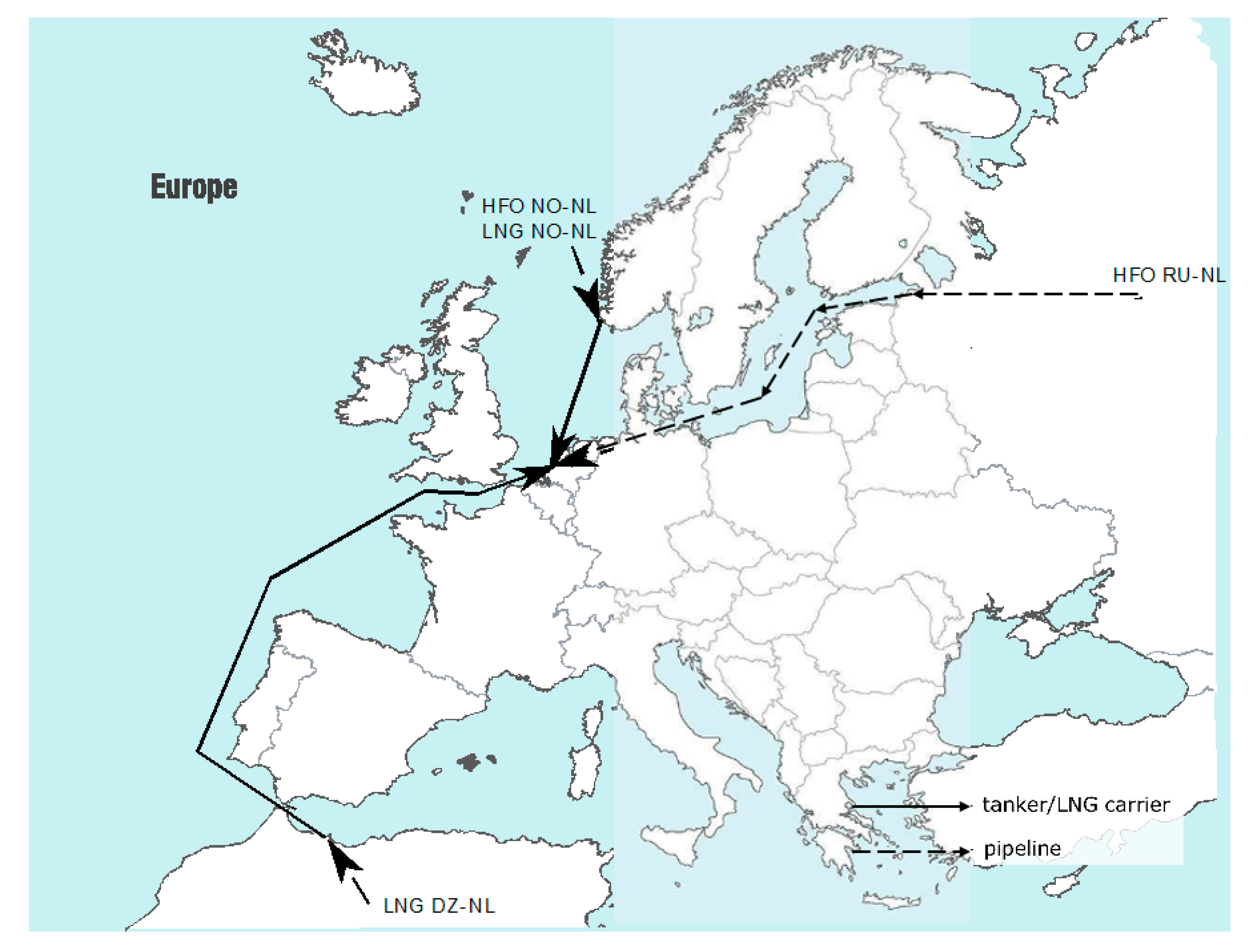
2.2. System Boundaries and Fuel Supply Chain Scenarios

The system boundaries, visualised in Figure 1 along with the investigated scenarios, include all processes from fuel extraction to its combustion. Aspects related to the products and services that affect the transport system but not directly related to the fuel are excluded, e.g., the infrastructure elements of the port and the vessels.
To understand how the inventory assumptions influence the LCA results, several realistic fuel supply chains were compiled and verified by literature, featuring various detail levels. Their geographical boundaries are presented in Figure 2, and their specifications are summarised in Table 3. Section 2.2.1 and Section 2.2.2 present in detail the scenarios and the assumptions for HFO and LNG, accordingly. The fuel supply chain of MDO was assumed to be identical to the one of HFO, except for the refinery process. To keep the focus on the comparison of HFO and LNG, only a generic fuel supply chain for MDO was considered.

2.2.1. HFO Supply Chain

Regarding HFO, a generic fuel supply chain base-case scenario was considered corresponding to average European data provided by ecoinvent v2.2 (named “RER”) [44]. In addition to the base case, two realistic fuel supply chains were composed. Assumptions were adopted regarding the country of crude oil extraction (both onshore and offshore cases were considered); the distances and modes of crude oil transport to the refinery; the refinery process; and the distribution of the refined fuel to the bunker station.
For the onshore extraction case, herein called HFO RU-NL, extraction occurs in Russia (RU) and transport occurs via pipeline, as it is the common case, at an average distance of 5200 km up to a refinery in the port of Rotterdam, Netherlands (NL). It is assumed that HFO is distributed by barge to the bunker station 20 km away. This corresponds to the distance between Gunvor refinery and a bunker station in the port Maasvlakte, situated at the entrance of the port of Rotterdam.
The offshore extraction case, herein called HFO NO-NL, considered an extraction of crude oil on Norwegian (NO) offshore platforms placed in the North Sea. The crude oil is assumed to be transported via an offshore pipeline from the troll oil field to Stavanger over 293 km and from there by tanker to Rotterdam, Netherlands (NL) over 463 km, to the same refinery as in the onshore case. For the distribution from refinery to the bunker station, the assumptions were the same as for the HFO RU-NL case.

2.2.2. LNG Supply Chain

For LNG, there is no generic fuel chain available in ecoinvent v2.2; therefore, the scenarios considered were based on specific realistic conditions.
For the onshore case, most of European LNG imports come from Qatar. However, given the lack of site-specific data, the corresponding data from Algeria (DZ) were used. The assumption is in line with other literature where LNG is considered to be extracted in Norway and Qatar [30]. In the present study, the natural gas onshore extraction case, herein called LNG DZ-NL, is placed in the Hassi R’Mel gas field. From there the natural gas is transported over 466 km to a liquefaction plant in Arzew. After liquefaction, the LNG is transported with an LNG carrier to Rotterdam, over 1963 km. Comparing Algeria and Qatar in terms of production, the liquefaction process is expected to be the same, while the difference between the two locations is seen in relation to transport: lower contribution of the pipeline and a higher contribution of the LNG carrier due to a longer distance from Qatar to Rotterdam.
For the offshore extraction case, herein called LNG NO-NL, natural gas was considered to be extracted in the North Sea at the Troll oil field, the same location as for the Norwegian crude oil extraction. The gas is transported via an offshore pipeline over 300 km to a liquefaction plant in Stavanger. The liquefaction process is considered to be the same for offshore and onshore cases due to the lack of specific data. From Stavanger the LNG is transported with an LNG carrier to Rotterdam over 462 km. For the LNG transport via an LNG carrier, a methane slip of 2% for both cases was considered [46].

2.3. Transport Specifications

For calculating fuel consumption, vessel operational profiles in terms of power demand and duration of each operational mode are taken into account (Table 4). For the container vessel, industrial data were adapted for European trade [49]. The tanker case is based on the study of Mountaneas (2014) [50]. The operational profile for the ferry and the cruise vessel cases was provided by DNV-GL and correspond to in-house data.

3. Results

The primary energy use and the GHG emissions for the upstream, Well-to-Tank, part of the system are given in Section 3.1. The values are provided per fuel energy content, in order to allow a direct comparison of different fuel options and supply chain scenarios. The results for the downstream, Tank-to-Propeller, part and for the overall, Well-to-Propeller, system are given in Section 3.2 and Section 3.3. The corresponding values are given per functional unit, which is vessel dependent, and therefore comparisons between vessels are not advisable. Cargo vessels such as containers and tankers have higher relative cargo capacity compared to passenger ships or ferries and therefore lower emissions and energy usage per functional unit. Different vessels offer different services; therefore, a direct comparison is not meaningful in LCA terms.

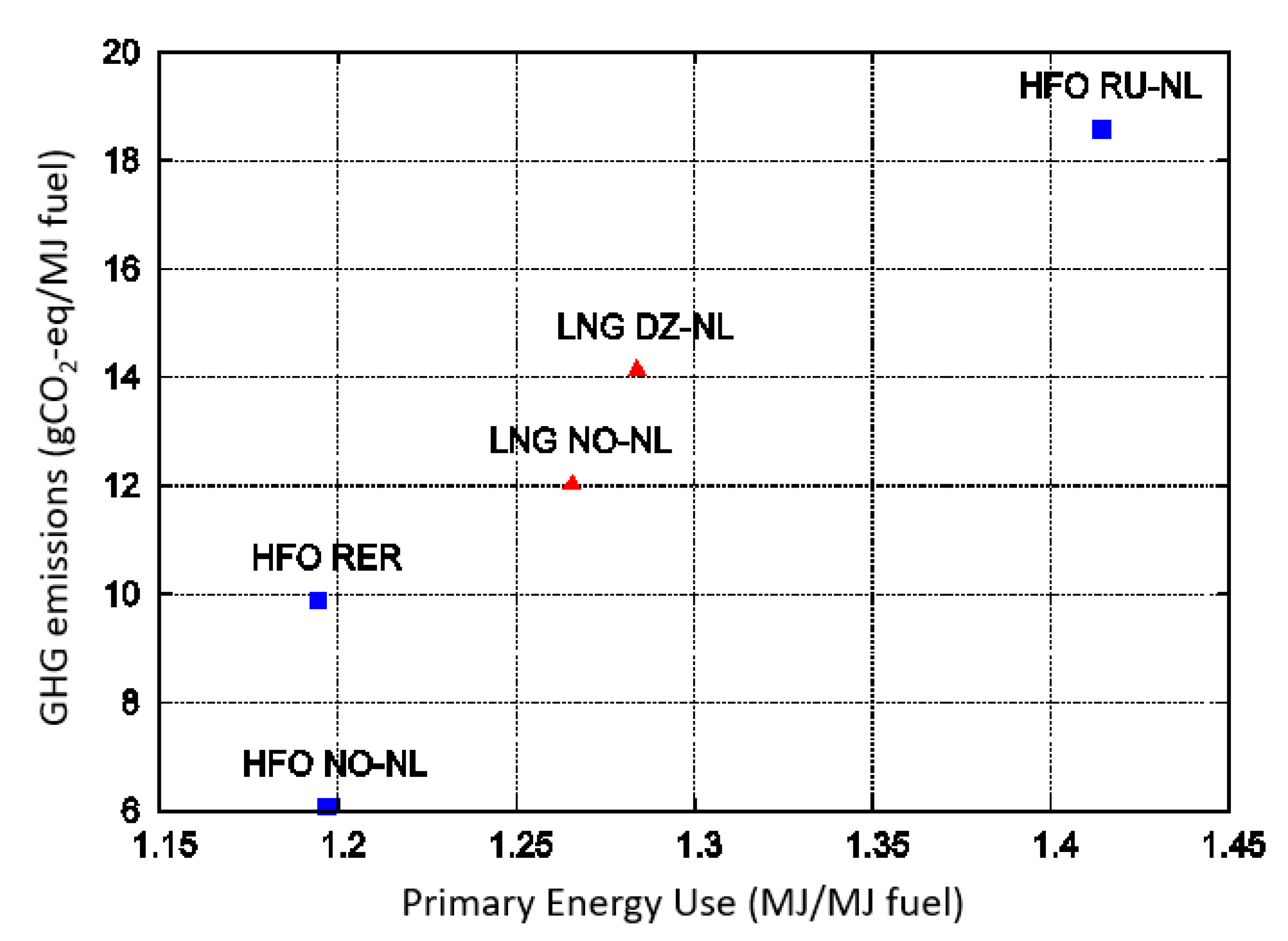
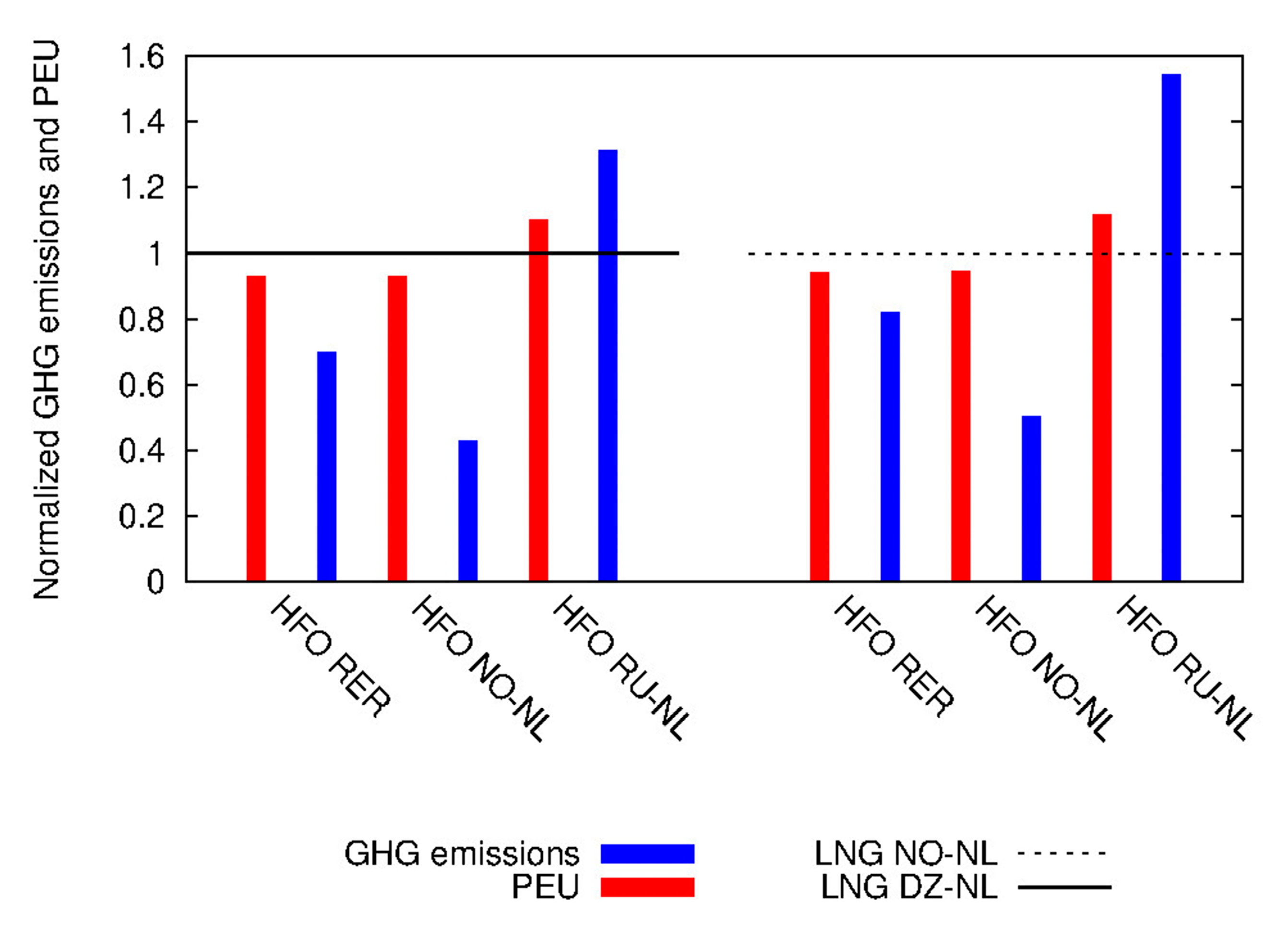
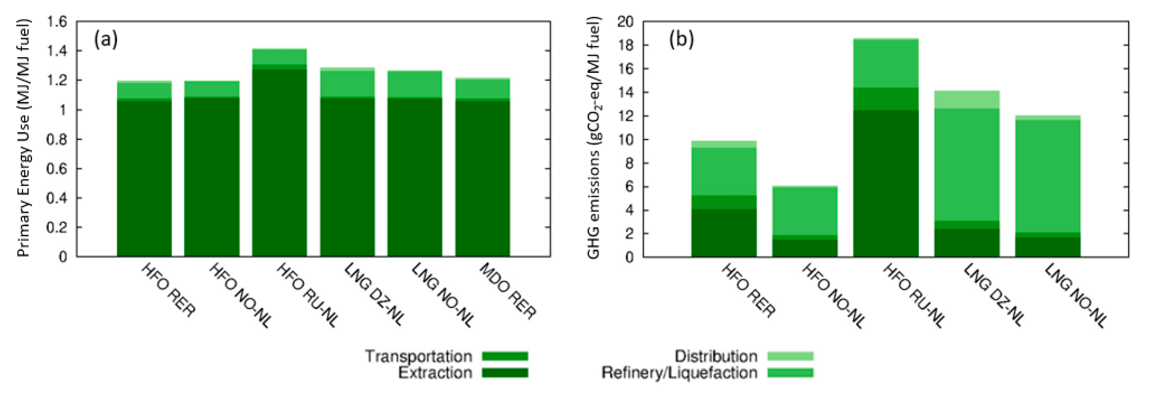
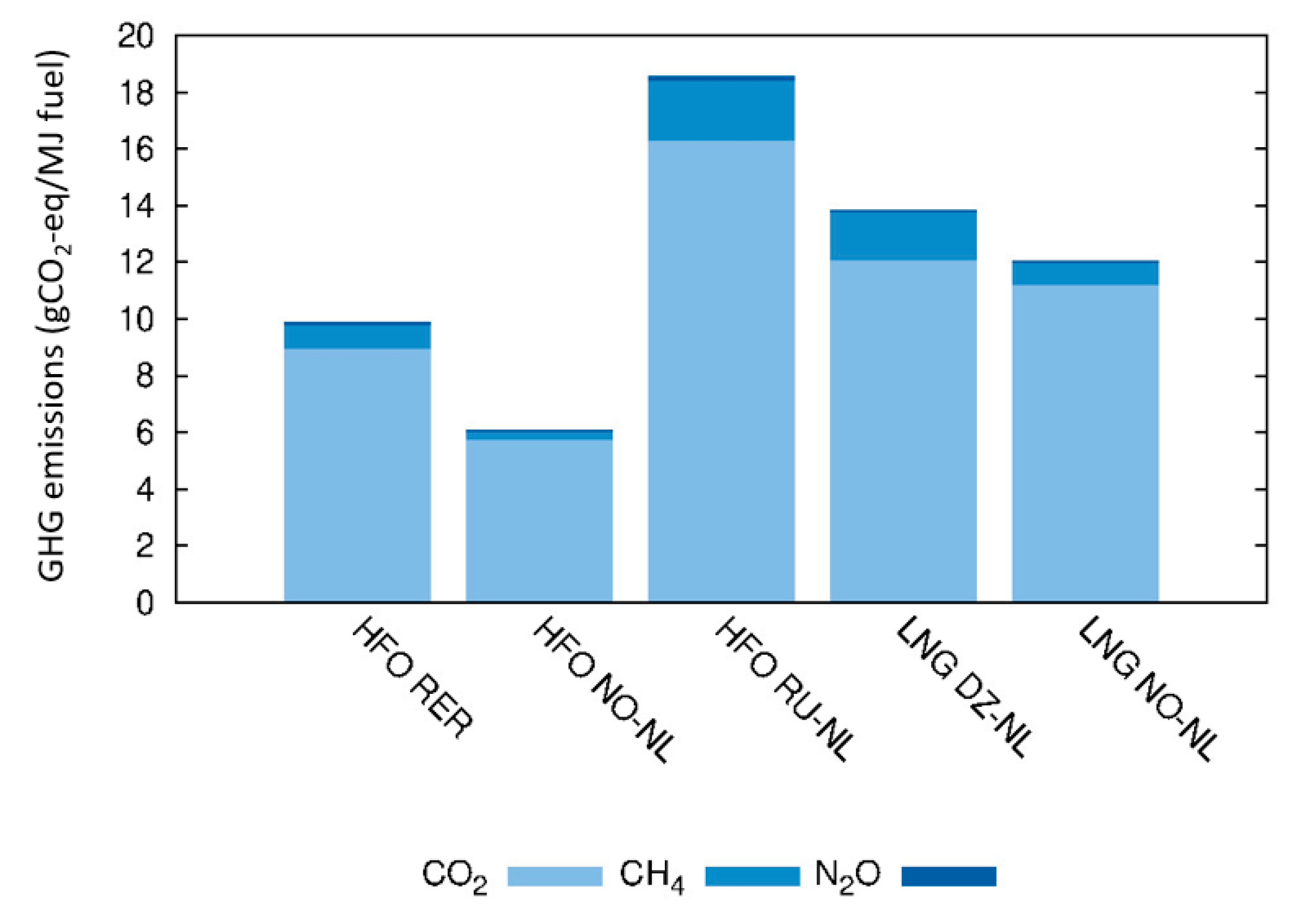
3.1. Upstream (Well-to-Tank)

The GHG emissions (gCO2-eq) and the primary energy use (MJ) per MJ fuel (based on a Lower Heating Value) at the bunker station are given in Figure 3. The HFO base-case fuel supply chain scenario (HFO RER) is found to be the most energy efficient. However, due to venting it is not the one with the lowest GHG emissions. Instead, the HFO extracted offshore in Norway (HFO NO-NL) has the lowest GHG emissions. The worst performing scenario for both indicators is the HFO extracted onshore in Russia (HFO RU-NL). These main results are further analyzed and explained in Section 3.1.1 (contribution analysis).
Figure 3 also allows us to compare the different scenarios regarding their emission intensity. It is shown that for HFO, the GHG emissions per MJ primary energy for the base-case average scenario (HFO RER) are 67% higher than the case of extraction in the North Sea (HFO NO-NL).
To better demonstrate the relationship between HFO and LNG, Figure 4 presents the fuel performance factors, meaning that the results for different HFO supply chains have been normalized by the LNG results for GHGs (in blue) and PEU (in red) for all scenarios. The left side of the figure corresponds to LNG supplied by Algeria, while the right side corresponds to LNG supplied by Norway. The figure shows that HFO is preferable to LNG except for the case when HFO extraction occurs in Russia (HFO RU-NL). It also shows that for LNG, the extraction point does not significantly affect the fuel’s performance. The results are further discussed in Section 4 in relation to other literature.

3.1.1. Contribution Analysis (Well-to-Tank)

Figure 5 shows the contribution of the different cradle-to-tank processes to the PEU and GHG emissions.
Regarding the PEU, raw material extraction is the main contributor to all fuel supply chain scenarios, accounting for approx. 90% of the total energy consumption. The primary energy requirement for the extraction of natural gas and crude oil is similar in all scenarios except for the HFO RU-NL where it is 18% higher. This is due to the lower energy efficient crude oil extraction in Russia (based on ecoinvent v2.2. data) and the longer transport distance of the crude oil to the refinery (see Table 3).
Regarding the GHG emissions, in contrast to the PEU, they differ significantly between the fuel supply chain setups with values ranging by 15% for the LNG cases and by 79% for the HFO ones.
For LNG, most of the impacts (67% and 79% for onshore and offshore, respectively) are due to the liquefaction process during which natural gas is burnt for energy production. For HFO the difference is due to crude oil extraction between the Russian and Norwegian scenarios, specifically in relation to:
  • Treatment of natural gas (NG) which is a byproduct of crude oil. Onshore (Russia) NG is either burned or directly vented which leads to direct methane emissions while offshore it is processed and further used. As Figure 6 shows, the methane contribution in the onshore case is 87% higher than in the offshore case. Most of it (90%) is due to the direct venting, and 6% is due to differences in refining. In the offshore case, extraction and refining emit the same amount of methane.
  • Capital equipment: the onshore plants have a lower productivity compared to the offshore platforms which implies higher infrastructure requirements per functional unit. Consequently, the corresponding GHG emissions are higher (approximately double).
Figure 6 presents the contribution of the different GHGs to the cradle-to-tank carbon footprint. Looking at this, the methane contribution onshore is 64% higher compared to offshore which is mainly due to methane slip during extraction (accounts for 49% of the cradle-to tank methane emissions) and transportation.

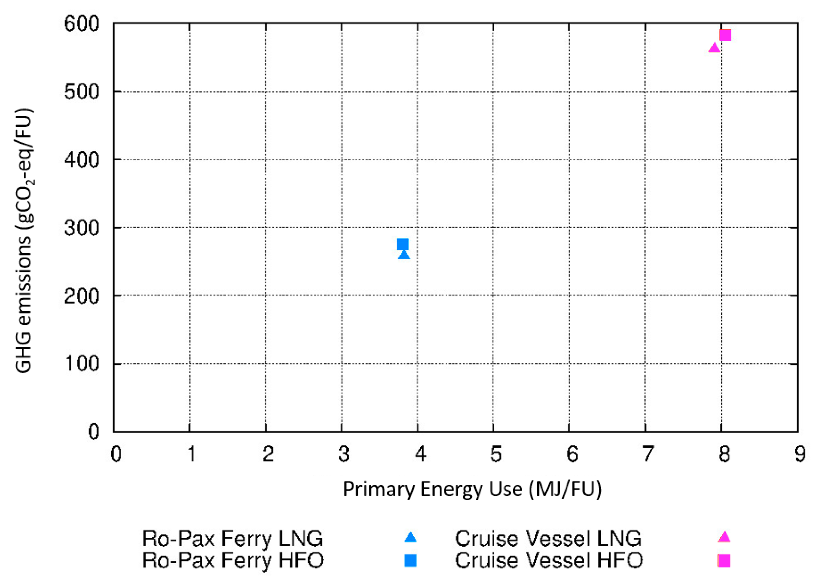
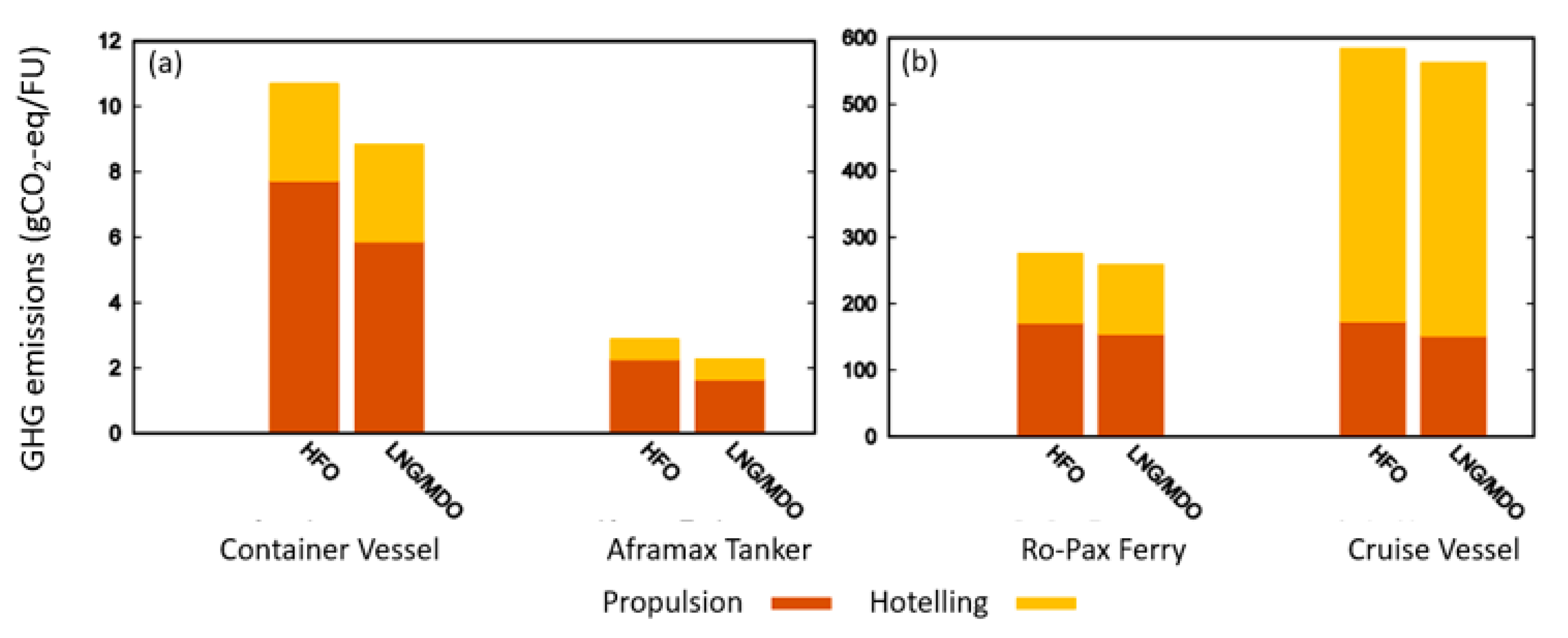
3.2. Downstream (Tank-to-Propeller)

The Tank-to-Propeller PEU and GHG emissions per functional unit for all vessels and both fuel alternatives are shown in Figure 7 and Figure 8.
Concerning PEU, the difference is rather insignificant and it is mainly related to the change in cargo capacity. Specifically, higher space demands for the LNG bunker lead to a reduction in cargo capacity for the container and ferry vessels. In contrast, cargo capacity remains unchanged for the tanker and the cruise vessels. Note that LNG is only used to fuel the main engines (ME) while the auxiliary ones (AE) use MDO for the coverage of hoteling demands. This means that the benefits from fuel transition are not fully exploited, which is particularly relevant for the vessels with high hoteling demands (see cruise vessels and ferries in Table 1). Specifically for the case of the ferry, which has both higher hoteling demands and lower cargo capacity (in comparison to the other vessel types), LNG performs marginally worse than HFO in terms of PEU.
Concerning GHGs, the highest benefit is seen in tankers, where the use of LNG leads to 50% fewer emissions. Contrary to the PEU, the GHG performance depends on the engine type installed. Four-stroke engines can perform 20% worse than two-stroke ones which is due to the different methane slip status of the two engine types (see Section 2.1). Similar to the PEU, the benefits from transitioning to LNG would be higher if it was not for the cargo capacity reduction (as in the case of the container and ferry) and the use of MDO for the secondary engines. To exemplify, Figure 9 shows the contribution of propulsion and hoteling to the total GHG emissions.
As mentioned at the beginning of Section 3, a direct comparison across vessels is not meaningful since the assessments use different functional units. However, it is of interest to rate the relative performance of the two fuels across vessels. The results in Table 5 show that LNG is preferable to HFO regarding both indicators and all scenarios.

3.3. Total System (Well-to-Propeller)

To derive the results for the total system “Well-to-Propeller”, the upstream “Well-to-Tank” and downstream “Tank-to-Propeller” parts of the system are combined.
In terms of Primary Energy Use (PEU), Table 6 shows that LNG is preferable only when the cargo capacity of the vessel remains unchanged. That is the case for tankers and cruise vessels. When the cargo capacity is reduced, as is the case for container vessels and ferries, LNG loses its competitive advantage over HFO. The difference between all studied scenarios is incremental (all results range from 1–3% except for HFO RU-NL where the difference is 3–10%). This implies that the PEU performance is similar for both fuels and engine types.
On the contrary, the spread of GHG emission results is greater (Table 7). The results for the HFO supply chain scenarios differ between them up to 10%. When transitioning to LNG, the GHG emissions are influenced by opposing drivers: on the one hand, the “cleaner” LNG supply chain, which gives an advantage over HFO, and on the other hand, a reduction in cargo capacity and a higher methane slip, that counterbalance this advantage. As a result, although LNG is beneficial for all cases, the benefit is higher for container and tanker vessels (10–30% GHG reduction) compared to cruise and ferries (1–10% GHG reduction).
Comparing the LNG supply chain alternatives, offshore transportation is preferable to onshore for both indicators. Overall, the worst scenario is the one for HFO extracted onshore in Russia HFO RU-NL: it is the least energy efficient and the greatest GHG emitting supply chain for all vessels.

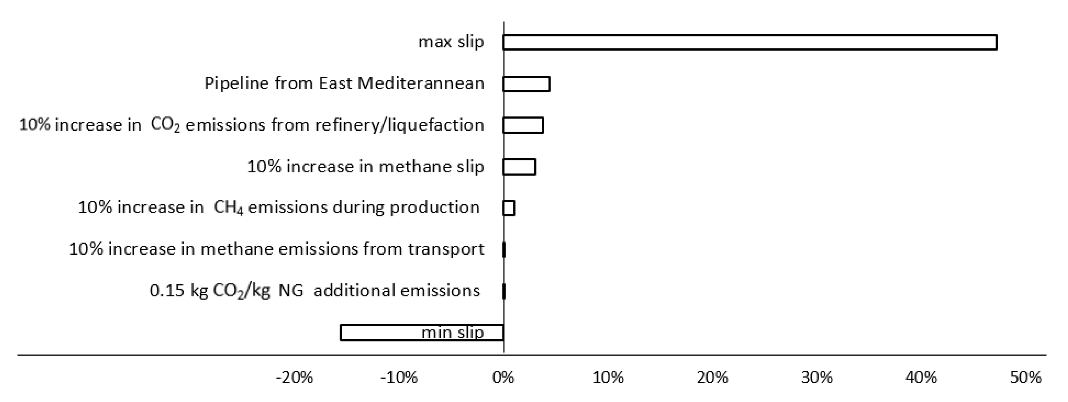
3.4. Sensitivity Analysis

The systems’ sensitivity to major assumptions, most influential and uncertain factors, was done through a scenario analysis. For the upstream part of the system, five scenarios (Table 8) were developed:
For the downstream part of the system, the sensitivity to methane slip from LNG-fueled vessels was tested. For the reference scenario, a 2% methane slip was considered. Taking the case of cruise vessels, this corresponds to 21 gCO2-eq which is in the range suggested by other literature for medium loads [55]. For the sensitivity analysis, the methane slip was assumed to range from 7 g to 36 g, corresponding to the findings of Anderson et al., (2015) who, based on measurements on-board a cruise ferry running on LNG with lean-burn dual fuel engines, showed that emissions due to methane slip (accounting for 85% of hydrocarbon emissions from LNG) were approximately 7 g per kg LNG at higher engine loads, rising to 23–36 g at lower loads [55].
All scenarios were tested ceteris paribus for the case of the LNG-fueled cruise vessel, which was chosen since the methane slip measured by Anderson et al., (2015) for the downstream part of the system corresponds to a similar vessel type [55]. The scenario analysis results are given in Figure 10. This tornado diagram allows us to see the relative importance of the factors and the system’s sensitivity to each of them ceteris paribus. The system is mostly sensitive to the methane slip downstream.

4. Discussion

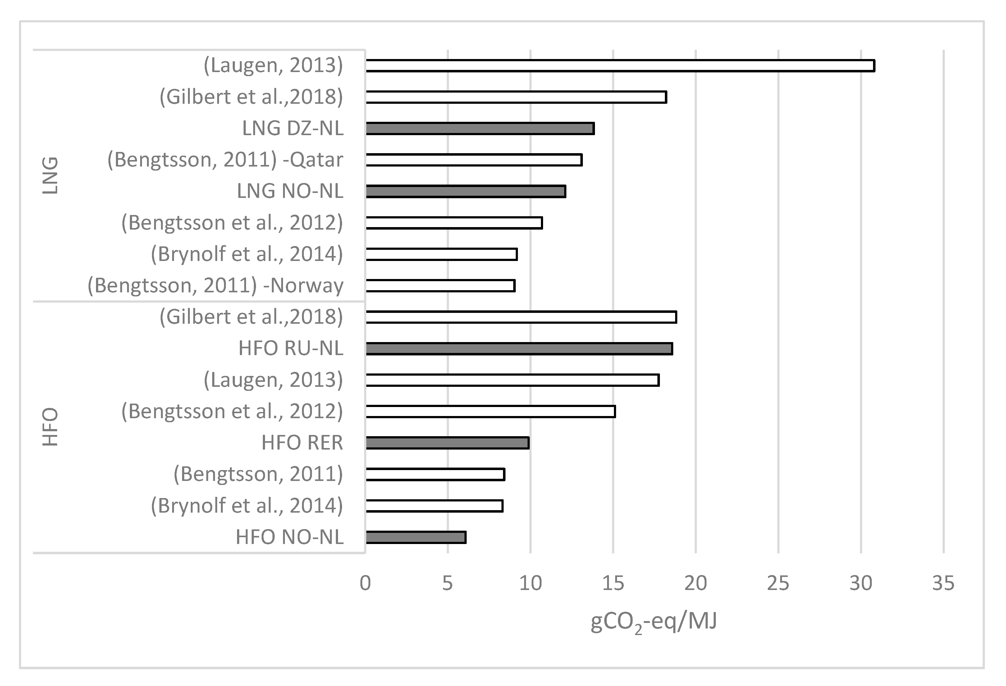
4.1. Comparison with Other Studies

To put this work in context, a comparison with other literature results has been performed.
For the upstream part of the system, Balcombe et al., (2018), after extensive review, list more than 25 emissions sources throughout six LNG supply chain stages (pre-production, extraction, gathering, processing, transmission, and storage, distribution) [51]. They then develop 160 emission scenarios and perform a Monte Carlo analysis which shows that typical facilities are estimated to emit 18–24 gCO2-eq./MJ Higher Heating value (HHV). Assuming that Lower Heating Value (LHV) is 96% of HHV, and that the methane global warming potential (GWP) is 25 CO2-eq (based on the IPCC fourth assessment report [56] instead of 34 assumed in Balcombe et al., (2018)), then the typical facilities are found to emit 16–21 gCO2-eq./MJ LHV, slightly higher than the results of the present study, i.e., 14.4 gCO2-eq./MJ LHV. The aforementioned analysis by Balcombe et al., (2018) concluded that mean estimates for the emissions from LNG supply chain range widely from 22g to 107 gCO2-eq./MJ HHV. This finding strengthens the finding of the present study that the use of generic data might jeopardise the accuracy of LCA results.
The results of the present study for the upstream, well-to-tank part of the system are further put in the context of the literature as seen in Figure 11.
The literature studies used for comparison are listed in Table 9 and have been selected due to the similar overall scope and technical system to the present study. However, they are not fully aligned (potentially different system description and boundaries, inventory data, modeling assumptions, impact assessment methodologies, level of detail in interpretation, etc.); thus, a direct comparison cannot be done. The same table presents the findings of other literature regarding the relative performance of LNG compared to HFO. The findings of the present study are given for the average of two-stroke (container vessel, tanker) and four-stroke (cruise vessel, ferry) engines. Note that only one study considered a two-stroke main engine [25]. Also, PEU is out of the scope in the aforementioned study [25] and therefore there are no entries from this literature source in the Table 9.
Regarding PEU all studies, including the present one, the results are a combination of two opposing drivers (a) the fuel supply chain, where all studies find LNG to be less energy efficient than HFO and (b) the energy consumption onboard where LNG is found to be more energy efficient than HFO.
Regarding GHG emissions, all studies find LNG to be preferable to HFO. The results of the present study deviate from other literature by 1–13%. This can be due to the fuel supply chain setup; to the combustion characteristics (e.g., emission factors and methane slip consideration), and to secondary services such as hoteling demands. Note that the average value of the GHGs of two-stroke engines found in this study matches the results of [25] for container vessels, the only study representing a two-stroke engine. Additionally, the results of Gilbert et al. (2018) [36], who consider generic data for the operation (e.g., for the engine type and the operational profile), correspond to the average results of two- and four-stroke engines found in the present study.
Even though all other studies have considered four-stroke engines, the contribution of methane matches the value found for two-stroke engines in the present study. Therefore, it is to be assumed that the methane slip for the four-stroke engines is underestimated in the literature. This is a point for further research since there is not enough detail in the considered studies to prove the assumption.

4.2. Policy Implications

The results of the present study demonstrate that multiple opposing drivers affect the environmental performance of maritime transport. This better understanding of the alternative marine fuel supply chains and the implications of fuel shifting is particularly relevant for policy makers and the maritime industry, in order to achieve more complete assessments and to avoid burden shifting.

4.2.1. The Need for Specific Fuel Supply Chains, Engine Types, and Operational Profiles

The results show how influential the inventory data are related to the extraction processes (location and processes such as the treatment of by-products) and to the methane slip. The latter depends on the type of engine and vessel’s operational profile, two aspects that commonly are beyond the scope of existing literature which can lead to an underestimation of methane slip. This finding calls for broadening the scope in future maritime transport LCA research.
The results also showed the influence of the vessels’ operational modes, which implies that use of generic data is unadvisable unless necessary. To exemplify, Figure 12 compares each case study against an aggregated benchmark derived for similar vessel types based on Automatic Identification System (AIS) data. Differences in the share of transit, manoeuvring, and port modes can be observed and are due to the individual characteristics of the assumed cases compared to the averaged results for the similar vessel types. For example, the ferry case corresponds a frequent service between islands with a short time at port during each trip, whereas the aggregated operational profile for ferries corresponds to longer times. This comparison shows that each different case is bound to a set of specifications which affects results. Therefore, in order to derive conclusions on the performance of different marine fuels in specific case studies, the use of the presented methodology, which accounts for specific operational profiles, is proposed.
The relative importance of different modes should be studied further in order to minimize adverse environmental impacts on a global (e.g. climate change) and local levels [4]. Additionally, as it is discussed in the following section, the relative contribution of the modes directly affects the Key Performance Indicators (KPIs) used for the environmental monitoring of the shipping industry.

4.2.2. A Call for LCA-Based Environmental Performance Indicators

The Energy Efficiency Operational Indicator (EEOI) introduced by the IMO as a monitoring tool for managing ship performance over time, regarding GHGs [59], does not have a life cycle perspective; therefore, it does not account for the upstream part of the system (fuel supply chains). Additionally, EEOI is measured in CO2 per transport unit, e.g., tkm; it thus covers only the CO2 proportion of the overall GHG emissions. When the vessels are fueled with HFO, this proportion reaches 99%. However, when the fuel is LNG, the representativeness is lower, since the methane slip is not accounted for. For example, in LNG-fueled four-stroke engines, the EEOI covers 90–94% of GHGs. The percentage would be lower if LNG would also be used in the auxiliary engines, instead of MDO. In cruise vessels, if the auxiliary engines were fueled with LNG, the contribution of CO2 to the total GHG emissions would be 83%. These findings call for more complete environmental performance indicators in the maritime sector so that all relevant substances (e.g., methane) and all life cycle stages are accounted for.

5. Conclusions

The innovation of the present study is that it accounts for the full maritime transport service including both fuel supply chains and propulsion considerations.
A ”Well-to-Propeller” LCA of maritime transport was performed with a European technological focus. Four typical types of vessels with specific operational profiles were considered and corresponding functional units assessed: a container vessel and a tanker, both with two-stroke engines (functional unit: 1 t of cargo transported for 1 km), a Ro-Pax ferry and a cruise vessel, both with four-stroke engines (functional unit: 1 passenger transported for 1 km). All main engines were dual fuel that can take either HFO or LNG with marine diesel oil (MDO) as a pilot fuel. Alternative realistic European fuel supply chains were considered for HFO (offshore production in Norway, onshore production in Russia) and for LNG (offshore production in Norway, onshore production in Algeria). The impact categories considered were climate change and primary energy use.
Raw material extraction was found to account for approx. 90% of the total energy consumption in all scenarios. Regarding CO2-eq emissions, liquefaction was found to be a hotspot across all scenarios. For HFO, crude oil extraction is also an emission hotspot mainly in relation to (a) treating the co-produced natural gas and (b) the requirements in infrastructure. Due to differences in these two aspects, the CO2-eq emissions between alternative HFO supply chains may differ by up to 79%.
When transitioning from HFO to LNG, the systems are influenced by (a) a reduction in cargo capacity due to bunkering requirements, (b) the fact that secondary engines required for covering hoteling demands are fueled by MDO, and (c) the methane slip which depends both on the fuels supply chain (onshore extraction has 64% greater slip compared to offshore) and on the engine type (four-stroke engines have 20% greater slip than two-stroke engines). As a result, LNG is more energy efficient than HFO only when the cargo capacity remains unchanged (the case of tankers and cruise vessels). When the cargo capacity is reduced, as is the case of container vessel and ferry (reduction by 1.8% and 4% respectively), LNG loses its competitive advantage. For GHGs, the combined effect of cargo capacity, engine type, and secondary fuel leads to LNG performing better than HFO only for the cases of two-stroke engines.
The present study also showed that the IMO suggested indicator for monitoring energy efficiency (EEOI) is suboptimal for addressing climate change. When the vessels are HFO-fueled the EEOI covers 99% of total GHGs. However, in the case of LNG fuel, the representativeness is lower since the methane slip is not accounted for (for four-stroke engines, the EEOI is 90–94% of GHGs). The gap between EEOI and GHGs would increase if LNG was used in the auxiliary engines.
The results thus demonstrate that multiple opposing drivers affect the environmental performance of maritime transport. This better understanding of marine fuel supply chains and the implications of fuel shifting is particularly relevant for policy makers, in order to avoid burden shifting and to establish better emission monitoring strategies.

Author Contributions

Conceptualization, M.F. and D.G.; methodology, D.G. and A.B.; software, G.J.S.; validation, A.B. and D.G.; formal analysis, G.J.S. and A.B.; investigation, G.J.S. and A.B.; resources, C.A.G.; data curation, G.J.S. and C.A.G.; writing—original draft preparation, A.B.; writing—review and editing, all authors; visualization, G.J.S.; supervision, D.G.; project administration, D.G.; funding acquisition, M.F. All authors have read and agreed to the published version of the manuscript.

Funding

This research was funded by the EUROPEAN COMMISSION, FP7 PEOPLE: MARIE-CURIE ACTIONS - INITIAL TRAINING NETWORK (ITN), Grant Agreement Nr 607214, project name: ECCO-MATE— Experimental and Computational Tools for Combustion Optimization in Marine and Automotive Engines.

Conflicts of Interest

The authors declare no conflict of interest. The funders had no role in the design of the study; in the collection, analyses, or interpretation of data; in the writing of the manuscript, or in the decision to publish the results.

References

  1. Sims, R.; Schaeffer, R.; Creutzig, F.; Cruz-Núñez, X.; D’Agosto, M.; Dimitriu, D.; Meza, M.J.F.; Fulton, L.; Newman, P.; Ouyang, M.; et al. Climate Change 2014: Mitigation of Climate Change. Contribution of Working Group III to the Fifth Assessment Report of the Intergovern- mental Panel on Climate Change; Edenhofer, O., Pichs-Madruga, R., Sokona, Y., Farahani, E., Kadner, S., Seyboth, K., Adler, A., Baum, I., Brunner, S., Eickemeier, P., et al., Eds.; Cambridge University Press: Cambridge, UK; New York, NY, USA, 2014; pp. 599–670. [Google Scholar]
  2. UNCTAD. Review of Maritime Transport Chapter 6: Sustainable Freight Transport—Development and Finance. United Nations Conference on Trade and Development, New York and Geneva, 2012. Available online: https://unctad.org/en/PublicationChapters/Chapter%206.pdf (accessed on 26 May 2020).
  3. Bouman, E.A.; Lindstad, E.; Rialland, A.I.; Strømman, A.H. State-of-the-Art Technologies, Measures, and Potential for Reducing GHG Emissions from Shipping—A Review. Transp. Res. Part D Transp. Environ. 2017, 52, 408–421. [Google Scholar] [CrossRef]
  4. Viana, M.; Hammingh, P.; Colette, A.; Querol, X.; Degraeuwe, B.; de Vlieger, I.; van Aardenne, J. Impact of Maritime Transport Emissions on Coastal Air Quality in Europe. Atmos. Environ. 2014, 90, 96–105. [Google Scholar] [CrossRef]
  5. Lin, H.; Tao, J.; Qian, Z.; Ruan, Z.; Xu, Y.; Hang, J.; Xu, X.; Liu, T.; Guo, Y.; Zeng, W.; et al. Shipping pollution emission associated with increased cardiovascular mortality: A time series study in Guangzhou, China. Environ. Pollut. 2018, 241, 862–868. [Google Scholar] [CrossRef] [PubMed]
  6. Russo, M.A.; Leitão, J.; Gama, C.; Ferreira, J.; Monteiro, A. Shipping emissions over Europe: A state-of-the-art and comparative analysis. Atmos. Environ. 2018, 177, 187–194. [Google Scholar] [CrossRef]
  7. EC. Reducing Emissions from Transport. Available online: https://ec.europa.eu/clima/policies/transport_en (accessed on 26 May 2020).
  8. Smith, T.W.P.; Jalkanen, J.P.; Anderson, B.A.; Corbett, J.J.; Faber, J.; Hanayama, S.; O’Keeffe, E.; Parker, S.; Johansson, L.; Aldous, L.; et al. Third IMO Greenhouse Gas Study 2014; The International Maritime Organisation: London, UK, 2015. [Google Scholar] [CrossRef] [Green Version]
  9. UNCTAD/RMT. Review of Maritime Transport 2016. United Nations Conference on Trade and Development, Geneva, 2016. Available online: https://unctad.org/en/PublicationsLibrary/rmt2016_en.pdf (accessed on 26 May 2020).
  10. IMO. International Convention for the Prevention of Pollution from Ships (MARPOL). Available online: http://www.imo.org/en/About/Conventions/ListOfConventions/Pages/International-Convention-for-the-Prevention-of-Pollution-from-Ships-(MARPOL).aspx (accessed on 14 July 2017).
  11. Cullinane, K.; Bergqvist, R. Emission Control Areas and Their Impact on Maritime Transport. Transp. Res. Part D Transp. Environ. 2014, 28, 1–5. [Google Scholar] [CrossRef]
  12. Marie Curie Actions (ITN, - Initial Training Network), G.A.N.; 607214. ECCO-MATE. Available online: http://ecco-mate.eu/ (accessed on 26 May 2020).
  13. IMO. Energy Efficiency Measures. Available online: http://www.imo.org/en/ourwork/environment/pollutionprevention/airpollution/pages/technical-and-operational-measures.aspx (accessed on 23 March 2018).
  14. IPCC. Summary for Policymakers. Climate Change 2013: The Physical Science Basis. Contribution of Working Group I to the Fifth Assessment Report of the Intergovernmental Panel on Climate Change; Stocker, T.F., Qin, D., Plattner, G.-K., Tignor, M., Allen, S.K., Boschung, J., Nauels, A., Xia, Y., Bex, V., Midgley, P.M., Eds.; Cambridge University Press: Cambridge, UK; New York, NY, USA, 2013. [Google Scholar]
  15. ISO. ISO 14044:2006. Environmental Management—Life Cycle Assessment—Requirements and Guidelines; International Organization for Standardization (ISO): Geneva, Switzerland, 2006. [Google Scholar]
  16. Frydendal, J.; Hansen, L.E.; Bonou, A. Environmental Labels and Declarations. In Life Cycle Assessment: Theory and Practice; Hauschild, M.Z., Rosenbaum, R.K., Olsen, S.I., Eds.; Springer International Publishing: Cham, Switzerland, 2018; pp. 577–604. [Google Scholar] [CrossRef]
  17. Bonou, A.; Laurent, A.; Olsen, S.I. Life Cycle Assessment of Onshore and Offshore Wind Energy-from Theory to Application. Appl. Energy 2016, 180, 327–337. [Google Scholar] [CrossRef] [Green Version]
  18. Prabhakaran, P.; Giannopoulos, D.; Köppel, W.; Mukherjee, U.; Remesh, G.; Graf, F.; Trimis, D.; Kolb, T.; Founti, M. Cost Optimisation and Life Cycle Analysis of SOEC Based Power to Gas Systems Used for Seasonal Energy Storage in Decentral Systems. J. Energy Storage 2019, 26, 100987. [Google Scholar] [CrossRef]
  19. Brynolf, S.; Magnusson, M.; Fridell, E.; Andersson, K. Compliance Possibilities for the Future ECA Regulations through the Use of Abatement Technologies or Change of Fuels. Transp. Res. Part D Transp. Environ. 2014, 28, 6–18. [Google Scholar] [CrossRef]
  20. Hua, J.; Wu, Y.; Chen, H. Alternative Fuel for Sustainable Shipping across the Taiwan Strait. Transp. Res. Part D Transp. Environ. 2017, 52, 254–276. [Google Scholar] [CrossRef]
  21. Abadie, L.M.; Goicoechea, N.; Galarraga, I. Adapting the Shipping Sector to Stricter Emissions Regulations: Fuel Switching or Installing a Scrubber? Transp. Res. Part D Transp. Environ. 2017, 57, 237–250. [Google Scholar] [CrossRef]
  22. Adom, F.; Dunn, J.B.; Elgowainy, A.; Han, J.; Wang, M.; Chang, R.; Perez, H.; Sellers, J.; Billings, R. Life Cycle Analysis of Conventional and Alternative Marine Fuels in GREETTM; Argonne National Laboratory: Argonne, IL, USA, 2013. [Google Scholar]
  23. Brynolf, S.; Fridell, E.; Andersson, K. Environmental Assessment of Marine Fuels: Liquefied Natural Gas, Liquefied Biogas, Methanol and Bio-Methanol. J. Clean. Prod. 2014, 74, 86–95. [Google Scholar] [CrossRef]
  24. Sames, P.; Clausen, N.B.; Lyder Andersen, M. Costs and Benefits of LNG as Ship Fuel for Container Vessels. Available online: http://marine.man.eu/docs/librariesprovider6/technical-papers/costs-and-benefits-of-lng.pdf?sfvrsn=18 (accessed on 26 May 2020).
  25. Thomson, H.; Corbett, J.J.; Winebrake, J.J. Natural Gas as a Marine Fuel. Energy Policy 2015, 87, 153–167. [Google Scholar] [CrossRef] [Green Version]
  26. Moirangthem, K. EC-JRC Techical Reports. Report EUR 27770EN. Alternative Fuels for Marine and Inland Waterways. An Exploratory Study; European Comission: Brussels, Belgium, 2016. [Google Scholar]
  27. Alvarez, R.A.; Pacala, S.W.; Winebrake, J.J.; Chameides, W.L.; Hamburg, S.P. Greater Focus Needed on Methane Leakage from Natural Gas Infrastructure. Proc. Natl. Acad. Sci. USA 2012, 109, 6435–6440. [Google Scholar] [CrossRef] [PubMed] [Green Version]
  28. IPCC. Climate Change 2014: Synthesis Report. Contribution of Working Groups I, II and III to the Fifth Assessment Report of the Intergovernmental Panel on Climate Change; Pachauri, R.K., Meyer, L.A., Eds.; IPCC: Geneva, Switzerland, 2014. [Google Scholar]
  29. Meyer, P.E.; Green, E.H.; Corbett, J.J.; Mas, C.; Winebrake, J.J. Total Fuel-Cycle Analysis of Heavy-Duty Vehicles Using Biofuels and Natural Gas-Based Alternative Fuels. J. Air Waste Manage. Assoc. 2011, 61, 285–294. [Google Scholar] [CrossRef] [PubMed]
  30. Bengtsson, S. Life Cycle Assessment of Present and Future Marine Fuels; Chalmers University of Technology: Gothenburg, Sweden, 2011. [Google Scholar]
  31. Corbett, J.J.; Winebrake, J.J. Emissions Tradeoffs among Alternative Marine Fuels: Total Fuel Cycle Analysis of Residual Oil, Marine Gas Oil, and Marine Diesel Oil. J. Air Waste Manage. Assoc. 2008, 58, 538–542. [Google Scholar] [CrossRef]
  32. Blanco-Davis, E.; Zhou, P. Life Cycle Assessment as a Complementary Utility to Regulatory Measures of Shipping Energy Efficiency. Ocean Eng. 2016, 128, 94–104. [Google Scholar] [CrossRef] [Green Version]
  33. Bengtsson, S.; Andersson, K.; Fridell, E. Life Cycle Assessment of Marine Fuels—A Comparative Study of Four Fossil Fuels for Marine Propulsion. Proc. Inst. Mech. Eng. Part M J. Eng. Marit. Environ. 2011, 225, 97–110. [Google Scholar] [CrossRef]
  34. Schönsteiner, K.; Massier, T.; Hamacher, T. Sustainable transport by use of alternative marine and aviation fuels—A well-to-tank analysis to assess interactions with Singapore’s energy system. Renew. Sustain. Energy Rev. 2016, 65, 853–871. [Google Scholar] [CrossRef]
  35. Hansson, J.; Månsson, S.; Brynolf, S.; Grahn, M. Alternative marine fuels: Prospects based on multi-criteria decision analysis involving Swedish stakeholders. Biomass Bioenergy 2019, 126, 159–173. [Google Scholar] [CrossRef]
  36. Gilbert, P.; Walsh, C.; Traut, M.; Kesieme, U.; Pazouki, K.; Murphy, A. Assessment of Full Life-Cycle Air Emissions of Alternative Shipping Fuels. J. Clean. Prod. 2018, 172, 855–866. [Google Scholar] [CrossRef]
  37. Mountaneas, A.; Georgopoulou, C.; Dimopoulos, G.; Kakalis, N.M.P. A Model for the Life Cycle Analysis of Ships: Environmental Impact during Construction, Operation and Recycling. MARTECH 2014, 2nd International Conference on Maritime Technology and Engineering. Lisbon. 2015, pp. 829–840. Available online: https://www.taylorfrancis.com/books/e/9780429226663/chapters/10.1201/b17494-89 (accessed on 26 May 2020). [CrossRef]
  38. Harris, I.; Sanchez Rodrigues, V.; Pettit, S.; Beresford, A.; Liashko, R. The Impact of Alternative Routeing and Packaging Scenarios on Carbon and Sulphate Emissions in International Wine Distribution. Transp. Res. Part D Transp. Environ. 2018, 58, 261–279. [Google Scholar] [CrossRef]
  39. Nocera, S.; Cavallaro, F. Economic Valuation of Well-To-Wheel CO2 Emissions from Freight Transport along the Main Transalpine Corridors. Transp. Res. Part D Transp. Environ. 2016, 47, 222–236. [Google Scholar] [CrossRef]
  40. Trivyza, N.; Rentizelas, A.; Theotokatos, G. A novel multi-objective decision support method for ship energy systems synthesis to enhance sustainability. Energy Convers. Manag. 2018, 168, 128–149. [Google Scholar] [CrossRef] [Green Version]
  41. Mansouri, S.A.; Lee, H.; Aluko, O. Multi-Objective Decision Support to Enhance Environmental Sustainability in Maritime Shipping: A Review and Future Directions. Transp. Res. Part E Logist. Transp. Rev. 2015, 78, 3–18. [Google Scholar] [CrossRef]
  42. EC-JRC. International Reference Life Cycle Data System (ILCD) Handbook—General Guide for Life Cycle Assessment—Detailed Guidance, 1st ed.; Publications Office of the European Union: Luxembourg, 2010. [Google Scholar] [CrossRef]
  43. Frischknecht, R.; Jungbluth, N.; Althaus, H.-J.; Doka, G.; Dones, R.; Heck, T.; Hellweg, S.; Hischier, R.; Nemecek, T.; Rebitzer, G.; et al. The Ecoinvent Database: Overview and Methodological Framework (7 Pp). Int. J. Life Cycle Assess. 2004, 10, 3–9. [Google Scholar] [CrossRef]
  44. SimaPro Software v.7; Pre-Consultants: Amersfoort, The Netherlands, 2007.
  45. FuelsEurope. Fuels Europe Statistical Report 2017. Available online: https://www.fuelseurope.eu/wp-content/uploads/2017/06/20170628-Graphs_FUELS_EUROPE-_2017_vFinal_WEB.pdf (accessed on 26 May 2020).
  46. DNV-GL. THE FUEL TRILEMMA: Next Generation of Marine Fuels. Available online: http://www.green4sea.com/wp-content/uploads/2015/06/DNV-GL-Position-Paper-on-Fuel-Trilemma.pdf (accessed on 26 May 2020).
  47. DNV-GL. LNG AS SHIP FUEL. Available online: https://www.dnvgl.com/Images/LNG_report_2015-01_web_tcm8-13833.pdf (accessed on 14 July 2017).
  48. DNV-GL. Costs and Benefits of Alternative Fuels. Available online: https://www.dnvgl.com/maritime/publications/alternative-fuels-study.html (accessed on 15 June 2017).
  49. Dimopoulos, G.G.; Georgopoulou, C.A.; Kakalis, N.M.P. Modelling and Optimisation of an Integrated Marine Combined Cycle System. In Proceedings of ECOS, the 25th International Conference on Efficiency, Cost, Optimization, Simulation and Environmental Impact of Energy Systems, Perugia, Italy, 26–29 June 2012; Firenze University Press: Firenze, Italy, 2012; pp. 4–7. [Google Scholar]
  50. Mountaneas, A. Life Cycle Assessment of Pollutants from Ships: The Case of an Aframax Tanker; Faculty of Mechanical, Maritime and Materials Engineering, TU: Delft, The Netherlands, 2014. [Google Scholar]
  51. Balcombe, P.; Brandon, N.P.; Hawkes, A.D. Characterising the Distribution of Methane and Carbon Dioxide Emissions from the Natural Gas Supply Chain. J. Clean. Prod. 2018, 172, 2019–2032. [Google Scholar] [CrossRef]
  52. EC/INEA. Eastern Mediterranean Natural Gas Pipeline—Pre-FEED Studies. Available online: https://ec.europa.eu/inea/en/connecting-europe-facility/cef-energy/7.3.1-0025-elcy-s-m-15 (accessed on 26 May 2020).
  53. EC/ENERGY. Projects of Common Interest—Interactive Map, European Union. 2019. Available online: http://ec.europa.eu/energy/infrastructure/transparency_platform/map-viewer/main.html (accessed on 26 May 2020).
  54. Jaramillo, P.; Griffin, W.M.; Matthews, H.S. Comparative Life-Cycle Air Emissions of Coal, Domestic Natural Gas, LNG, and SNG for Electricity Generation. Environ. Sci. Technol. 2007, 41, 6290–6296. [Google Scholar] [CrossRef] [PubMed]
  55. Anderson, M.; Salo, K.; Fridell, E. Particle- and Gaseous Emissions from an LNG Powered Ship. Environ. Sci. Technol. 2015, 49, 12568–12575. [Google Scholar] [CrossRef]
  56. Solomon, S.; Intergovernmental Panel on Climate Change.; Intergovernmental Panel on Climate Change. Working Group I. In Climate Change 2007: The Physical Science Basis: Contribution of Working Group I to the Fourth Assessment Report of the Intergovernmental Panel on Climate Change; Cambridge University Press: Cambridge, UK, 2007. [Google Scholar]
  57. Laugen, L. An Environmental Life Cycle Assessment of LNG and HFO as Marine Fuels; NTNU: Trondheim, Sweden, 2013. [Google Scholar]
  58. Bengtsson, S.; Fridell, E.; Andersson, K. Environmental Assessment of Two Pathways towards the Use of Biofuels in Shipping. Energy Policy 2012, 44, 451–463. [Google Scholar] [CrossRef]
  59. IMO. MEPC.1/Circ.684: Guidelines for Voluntary Use of the Ship Energy Efficiency Operational Indicator (Eeoi); International Maritime Organisation: London, UK, 2009. Available online: https://gmn.imo.org/wp-content/uploads/2017/05/Circ-684-EEOI-Guidelines.pdf (accessed on 26 May 2020).
Figure 1. System boundaries.
Energies 13 02739 g001
Figure 2. Indicative layout of the representative fuel supply chain routes in Europe.
Energies 13 02739 g002
Figure 3. Cradle-to-tank GHG emissions and PEU per MJ fuel at the bunker station.
Energies 13 02739 g003
Figure 4. Trends for GHG emissions and PEU for different HFO supply chains normalized by the related LNG supply chain outputs.
Energies 13 02739 g004
Figure 5. Contribution of modelled fuel supply chain processes to cradle-to-tank: (a) Primary Energy Use; (b) GHG emissions.
Energies 13 02739 g005
Figure 6. Contribution of the different GHGs to the cradle-to-tank GHG footprint.
Energies 13 02739 g006
Figure 7. Tank-to-propeller GHG emissions and PEU per tkm for two-stroke engines.
Energies 13 02739 g007
Figure 8. Tank-to-propeller GHG emissions and PEU per pkm for four-stroke engines.
Energies 13 02739 g008
Figure 9. Contribution of Propulsion and Hoteling demands to the tank-to-propeller GHG emissions: (a) two-stroke-engines; (b) four-stroke-engines.
Energies 13 02739 g009
Figure 10. Change (%) of Life Cycle GHG emissions due to the scenario analysis (ceteris paribus).
Energies 13 02739 g010
Figure 11. Comparison between results found in other literature and in the present study for the well-to-tank part of the system.
Energies 13 02739 g011
Figure 12. Comparison of operational profiles from AIS and case studies.
Energies 13 02739 g012
Table 1. Vessel specifications based on DNV GL inhouse data.
Vessel Type Container VesselTankerFerryCruise Vessel
Main
Engine
Engine type(-)2 stroke DF engine4 stroke DF engine
Power output(kW)1 × 37,6801 × 14,9402 × 3180 3 × 5300
Auxiliary
Engine
Engine type(-)4 stroke diesel engine
Power output(kW)2 × 22051 × 22052 × 22053 × 2205
Cargo capacity(-)4500 TEU105,000 ton800 passengers, 130 cars or 15 trucks2510 PAX
Freight load factor to DWT/PAX for HFO (LNG)(-)0.7 (0.69)0.75 (0.75)0.75 (0.72)0.81 (0.81)
Dead weight(DWT)67,567114,82914404042
Service speed(kn)24.5141921
Unit explanation: Dead weight (DWT), Passenger capacity (PAX), Twenty foot-equivalent (TEU).
Table 2. Fuel properties based on ecoinvent v2 as implemented in SimaPro software v.7.
PropertyUnitHFOLNGMDO
Lower Heating Value (LHV)(MJ/kg)42.74842.7
Density(kg/m3)930455 (NG 0.8)882
Emission factors CO2 (g/MJ)72.155.272.1
CH4 (g/MJ)0.0290.0450.029
N2O (g/MJ)0.001870.0010.00187
CO2-eq (g/MJ)72.755.672.7
Table 3. Specification of geographical boundaries.
Scenario Name *Extraction Transport Refinery (R)/Liquefaction (L)Distribution to Bunker Station
HFO RU-NLOnshore Russia (RU)Onshore pipeline 5200 km(R) RotterdamBarge 20 km
HFO NO-NLOffshore North Sea (Troll field), Norway (NO)Offshore pipeline from Troll field to Stavanger (293 km)
Tanker from Stavanger to Rotterdam (462 km)
(R) RotterdamBarge 20 km
LNG DZ-NLOnshore Algeria (DZ), Hassi R’Mel gas fieldOnshore pipeline from Hassi R’Mel gas field to Arzew (DZ) (466 km)(L) ArzewLNG carrier Arzew-Rotterdam (1618 km)
LNG NO-NLOffshore North Sea (Troll field), NOOffshore pipeline from Troll field to Stavanger (293 km)(L) StavangerLNG carrier Stavanger-Rotterdam (463 km)
* The scenario name corresponds to “Fuel type-Country of extraction-Country of port location”.
Table 4. Operational profiles of investigated vessels.
Vessels and Operational ModesSpeedDurationDistancePropulsionHotelling
(kn)(h)(km)(kW)(kW)
2-strokeContainer vesselHigh speed 25101457431,0593060
Normal speed19215746123,7513060
Ballast transit13222532716,4431530
Manoeuvring10134251112,7893130
Port0202003060
TankerNormal speed145358138,92210,039717
Manoeuvring534231673586717
Port00001004
4-strokeFerryDesign speed31910656002660
Manoeuvring171320001900
Port2000950
Cruise vesselCruise 112103322,95745336396
Cruise 214133934,71869256396
Transit 11676522,66899986396
Transit 21857419,13513,8236396
Manoeuvring531529174086396
Port03375006396
Table 5. Trends of different fuel scenarios for tank-to-propeller GHG emissions and PEU.
Vessel Type% Change in Primary Energy Use When LNG Is Used Instead of HFO% Change in GHG Emissions when LNG Is Used Instead of HFO
Propulsion OnlyPropulsion and HotelingPropulsion OnlyPropulsion and Hoteling
Container vessel−2%−2%−28%−17%
Tanker−7%−6%−31%−21%
Ferry−2%0%−12%−6%
Cruise vessel−6%−2%−15%−4%
Table 6. Trends for Well-to-Propeller PEU for different case setups using different fuel supply chains of HFO normalized by the two LNG case setup outputs.
Vessel Type% Change in Primary Energy Use when LNG is Used Instead of HFO
Using LNG (Supplied by Algeria) Instead of HFO Supplied by Three Alternative Sources:Using LNG (Supplied by Norway) Instead of HFO Supplied by Three Alternative Sources:
Average
European
From NorwayFrom RussiaAverage
European
From NorwayFrom Russia
Container1%1%−6%0%0%−7%
Tanker−3%−3%−11%−3%−4%−12%
Ferry3%−3%−3%2%−2%−4%
Cruise−1%−1%−4%−1%−1%−4%
Table 7. Trends for Well-to-Propeller GHG for different case setups using different fuel supply chains of HFO normalized by the two LNG case setup outputs.
Vessel Type% Change in GHGs when LNG Is Used Instead of HFO
Using LNG (Supplied by Algeria) Instead of HFO Supplied by Three Alternative Sources:Using LNG (Supplied by Norway) Instead of HFO Supplied by Three Alternative Sources:
Average
European
From NorwayFrom RussiaAverage
European
From NorwayFrom Russia
Container−13%−9%−22%−15%−11%−24%
Tanker−19%−15%−29%−21%−17%−31%
Ferry−1%2%−8%−2%1%−9%
Cruise−2%−1%−5%−3%−1%−6%
Table 8. Assumptions related to the upstream part of the system that were tested through a scenario analysis.
Tested Assumption and Reference ValuesDeveloped ScenarioReasoning
Methane emissions from LNG production 10% increase This life cycle stage is both impactful and uncertain.
Methane emissions from LNG transmission10% increase This assumption was found to be a hotspot in other literature [36,38,51].
Pipeline distance2700 km onshore 1000 km offshoreThe scenario corresponds to the latest policy plans for a pipeline from east Mediterranean (EastMed project) [52]. The pipeline distance accounting for existing and new pipelines is estimated to the port of Rotterdam [53].
Carbon emissions from refinery/liquefaction10% increase This life cycle stage was found to be the most impactful accounting for more than 50% of CO2 emissions. Note that the CO2 intensity of liquefaction in the reference scenario (0.4 kgCO2eq/kg LNG) is close to the average (0.6 kgCO2-eq/kg LNG) reported in the literature [54].
Carbon emissions from refinery/liquefactionIncrease by 0.15 kg CO2/kg NG Following the example of [36], this scenario accounts for additional emissions due to venting and flaring.
Table 9. Case studies used for comparison.
StudyVessel TypeEngine TypeGeographical Boundaries% Change in GHG When LNG Is Used Instead of HFO% Change in PEU When LNG Is Used Instead of HFO
Present studyAverage of cruise and ferryFour-strokeEurope−3%−1%
Average of container and tankerTwo-strokeEurope−16%−3%
[25] TugFour-strokeEurope−9%N/A
[25]Container Two-strokeNorth America−16%N/A
[57]FerryFour-strokeEurope−2%−27%
[23]FerryFour-strokeEurope−7%4%
[30]FerryFour-strokeEurope−10%9%
[58]FerryFour-strokeEurope−16%10%
[36]Not specifiedNot specifiedEurope−8%N/A

