An Operational Approach to Multi-Objective Optimization for Volt-VAr Control

Abstract

Recent research has enabled the integration of traditional Volt-VAr Control (VVC) resources, such as capacitor banks and transformer tap changers, with Distributed Energy Resources (DERs), such as photo-voltaic sources and energy storage, in order to achieve various Volt-VAr Optimization (VVO) targets, such as Conservation Voltage Reduction (CVR), minimizing VAr flow at the transformer, minimizing grid losses, minimizing asset operations and more. When more than one target function can be optimized, the question of multi-objective optimization is raised. In this work, a general formulation of the multi-objective Volt-VAr Optimization problem is proposed. The applicability of various multi-optimization techniques is considered and the operational interpretation of these solutions is discussed. The methods are demonstrated using a simulation on a test feeder.

1. Introduction

Traditional distribution systems include Volt-VAr Control (VVC) devices that aim to maintain the voltage within allowable limits, as required by the grid code or by power quality standards, such as EN 60150 [1,2]. Failure to meet these limits may result in regulatory sanctions and fines and, in extreme cases, malfunction and damage to electrical equipment.

The load fluctuates during the day as a function of a number of variables, such as the type of load, the type of infrastructure, geographical area, local weather conditions, season, holidays and so on [3]. There are methods in which a VVC device varies the reactive power, which consequently also changes the voltage in the system. These are called indirect VVC methods, and these include devices such as shunt reactors, capacitor banks, Static VAr Compensators (SVC) and (more recently) distributed generators (DG). Meanwhile, direct methods can directly change and affect the voltage and include devices such as On-Load Tap Changers (OLTC), transformers and voltage regulators [4].

Until the last decade, due to the lack of telemetry at the distribution network, the methods used to dynamically control voltage levels were very basic and mostly relied on connecting and disconnecting capacitor banks [5]. Recent smart grid technologies gather a vast amount of data and information for electricity utilities. On the one hand, this amount of data increases the complexity of the analysis required for the decision-making process; on the other hand, it allows for more sophisticated, dynamic and holistic methods of controlling voltage levels—a process which is usually referred to as Volt-VAr Optimization (VVO) [6,7,8,9].

The operation of the DG consumes energy resources and increases the operational age of the machine. Voltage control coordination is therefore necessary in the distribution network and has been a subject of interest in many research papers. For example, Ma et al. in [10] used the hierarchical genetic algorithm (HGA) to optimize a power and voltage control system according to the number of control actions. In [11], an integrated voltage control method, called Coordinated Secondary Voltage Control (CSVC), was proposed to control the LTC positions to ensure that voltage and loading constraints were satisfied during normal and emergency conditions. Practical VVC applications must take into consideration some physical and economical aspects of the assets [12]. Some work has been done on the coordination and operation of VVC assets under various conditions. Meanwhile, other studies have focused on the coordination of DGs and LTCs [13]. Another approach considered in the literature is distributed control through multi-agent systems (see [14]), as well as, more recently, hybrid control, in which both centralized and distributed optimization is done [9].

The addition of VVO may add other capabilities to the system, such as reduced system losses, reduced transformer losses and the control of the reactive power flow up to zero or even negative VAr flow and flat voltage profiles. Recently, a holistic method based on control at a system level of the volt-VAr assets, with the aim of achieving one of seven possible target functions, was proposed in [15]. This raises the need for multi-objective optimization, where more than one target function is optimized and where the target functions may contradict each other.

Multi-objective optimization (MOO) is a well-established area of research. MOO was probably introduced in the 1960s by Geoffrion [16], but its roots lie in much earlier research; for example, see the historical review and extensive survey in [17]. MOO approaches can mainly be divided into two categories: classical ones and metaheuristics [18]. The latter have been more widely used because they are capable of providing good solutions within a reasonable computation time. Many researchers have provided comprehensive surveys on metaheuristics, such as the works presented in [19,20,21,22] and very recently the work in Liu et al. [23]. Many textbooks have been, and still are being, written on the subject, such as the work presented in [24,25] and more recently in [26]. MOO methods have also been widely applied in areas related to VVC, such as the multi-objective planning of distributed energy resources [27] and multi-objective optimization of a stand-alone hybrid renewable energy systems [28].

In the last decade, following the smart-grid revolution, some works in the VVC literature have addressed some aspects of MOO. The first researchers to mention multi-objective tradeoffs were probably Turitsyn et al. [29], who discussed the tradeoff between power quality (which is usually achieved by increasing the reactive power Q) and distribution loss reduction (which requires minimal Q). In [30], the authors also consider active power losses and voltage deviations and use a weighing function to combine the two without addressing the question of how to select the weights. In [31], the authors also consider loss minimization and how to reduce voltage variation. They propose the avoidance of the problem of choosing weights with a switching law that evaluates the state of the system and determines which objective function best meets the current system needs. Recently, in [32], the authors proposed an adaptive weight-sum algorithm to solve a similar problem in a robust manner. Some works have addressed other target functions. For example, in [33], power loss, voltage profile, and voltage stability are considered. A genetic algorithm is used to find all Pareto-optimal solutions, which are then ranked using a fuzzy compromise function. In [31], the multiple objectives of the VVC problem are to minimize the electrical energy losses, voltage deviations, total electrical energy costs and total emissions of renewable energy sources and the grid, and a fuzzy function is used to combine the multiple target functions. A similar fuzzy membership function is used in [34] to optimize the energy loss, total switched capacitor reactive power and total number of daily switching operations. Voltage variation on pilot buses, reactive power production ratio deviation and generator voltage deviation are minimized in [35,36]. In both cases, the multiple objectives are addressed using the weighted-sum of Pareto-optimal solutions. Total energy costs, energy losses, emissions produced and voltage deviations are considered in [37]. Generally, these studies focus on the very important problem of solving a specific VVC–MOO problem, but none of them propose a general framework for formulating such a problem.

While multi-objective tradeoffs are becoming common in distribution systems and several solutions have been proposed, the adoption level of these solutions is very low. To the best of the authors’ knowledge, no operational system exists for multi-objective optimization in distribution networks. One of the main reasons for this is the lack of operational interpretation. A solution may be mathematically valid, but it will be difficult to adopt without clear operational interpretation. The contributions of this work are therefore as follows:

• A general framework for formulating multi-objective Volt-VAr Optimization problems is proposed. Such a model has not been proposed before. The manner in which previous work on VVC–MOO can be expressed in terms of this framework is shown.
• More importantly, the application of simple techniques for MOO on VVC problems is investigated, and the operational interpretation of each of these techniques is discussed. This discussion of operational interpretation is novel to this field and is missing from previous work on VVC–MOO. This discussion, especially when the operational interpretation is intuitive, may lead to the faster adoption of these techniques.

The structure of this paper is as follows. First, in Section 2.1, a general formulation for multi-objective Volt-VAr Optimization problems is proposed. This formulation serves as the fundamental block for the MOO techniques that are discussed in Section 2.2, and an operational interpretation for each is provided. Then, in Section 3, these methods are applied and demonstrated on a test feeder, optimizing active power and reactive power. This is followed by the presentation of conclusions in Section 4.

2. Materials and Methods

2.1. General Multi-Objective Volt-VAr Optimization

In this section, a general formulation for the VVO problem is proposed. The section begins with a general formulation of the single-objective variant. This is followed by a brief discussion on the subject of time and scenario-based optimization. Next, the formulation is extended to the multi-objective case. This formulation is based on the work in [15] but extends it considerably.

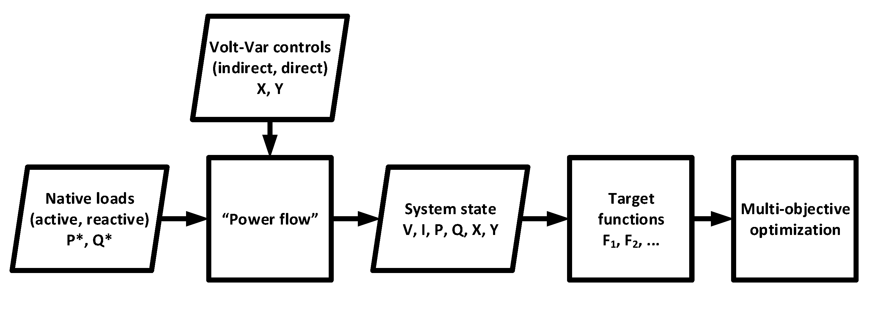
The proposed process of the modeling approach is illustrated in Figure 1. Using standard flowchart symbols, data are presented in parallelograms, and functions are presented in rectangles. From left to right, the process starts with the active and reactive native loads, $P^{*}$ and $Q^{*}$. The controls of the system are indirect and direct controls, X and Y. Using power flow mechanisms, the system state can be calculated. The system state is expressed in terms of the voltages V, the currents I, the loads P and Q and the controls X and Y. It is proposed that all target functions $F_1,F_2,\dots$ should be expressed using the system state $(V,I,P,Q,X,Y)$. Multi-objective optimization can then be used to combine these target functions.

2.1.1. The General VVO Problem

Let $k=1,\dots ,K$ be the nodes (buses) of the network and let $j=1,\dots ,J$ be the conductors (edges) of the network. Let $\{P_k^{*},Q_k^{*}\}$ be the native active and reactive power consumption in leaf node k, with vector notation $\{\overrightarrow{P^{*}},\overrightarrow{Q^{*}}\}$.

Considering both indirect and direct voltage control elements, let $a=1,\dots ,A$ be the indirect voltage control elements. Each control element a is associated with decision variable $X_a\in {\xi }_a$, where ${\xi }_a$ are the possible values of $X_a$, with vector notation $\overrightarrow{X}$. Note that $\overrightarrow{X}$ may be discrete (e.g., in capacitor banks, which can usually be connected or disconnected) or continuous (e.g., smart inverters). In either case, the function g associates the control vector $\overrightarrow{X}$ and the native active and reactive power vectors $\{\overrightarrow{P^{*}},\overrightarrow{Q^{*}}\}$ with the actual active and reactive power consumption $\{\overrightarrow{P^{\prime }},\overrightarrow{Q^{\prime }}\}$, as follows:

$$\{\overrightarrow{P^{\prime }},\overrightarrow{Q^{\prime }}\}=g(\overrightarrow{X},\overrightarrow{P^{*}},\overrightarrow{Q^{*}}).$$

(1)

Similarly, let $b=1,\dots ,B$ be the direct voltage controlled elements. Each controlled element b is associated with decision variable $Y_b\in {\psi }_b$, where ${\psi }_b$ are the possible values of $Y_b$ with vector notation $\overrightarrow{Y}$. Note that ${\psi }_b$ are voltages and may also be continuous or discrete. For example, an LTC is discretely controlled, while a voltage regulator may have continuous control.

From the actual active and reactive power consumption $\{\overrightarrow{P^{\prime }},\overrightarrow{Q^{\prime }}\}$ and the direct voltage controls Y, the voltages $V_k$ and currents $I_j$ ($\overrightarrow{V}$ and $\overrightarrow{I}$) can be calculated, as well as the total active and reactive power $\{\overrightarrow{P},\overrightarrow{Q}\}$. This is usually done by solving the well-known power flow equations

$$\begin{array}{ccc}\hfill P_m& =Re\left[\sum _{n=1}^K{V}_m{V}_n^{*}{\mathbf{Y}}_{m,n}^{*}\right]\hfill & \hfill m=1,\dots ,K\end{array}$$

(2)

$$\begin{array}{ccc}\hfill Q_m& =Im\left[\sum _{n=1}^K{V}_m{V}_n^{*}{\mathbf{Y}}_{m,n}^{*}\right]\hfill & \hfill m=1,\dots ,K\end{array}$$

(3)

where $\mathbf{Y}$ is the admittance matrix that represents the topology; that is, ${\mathbf{Y}}_{m,n}$ is the admittance between buses m and n. After the equations are solved, the current can be easily calculated from the voltages and line admittances.

This process is denoted $\mathbb{PF}$:

$$\{\overrightarrow{V},\overrightarrow{I},\overrightarrow{P},\overrightarrow{Q}\}=\mathbb{PF}(\overrightarrow{P^{\prime }},\overrightarrow{Q^{\prime }},\overrightarrow{Y}).$$

(4)

Note that the term “power flow” is used in this work, but this does not necessarily need to be the case, and any other form of voltage, current and power evaluation will suffice. For example, in some works about balanced networks, approximations are used.

For simplicity, and without loss of generality, the general single-objective VVO problem is defined as a minimization problem of a function f, under constraints:

$$\begin{array}{cc}\hfill min& f(\overrightarrow{V},\overrightarrow{I},\overrightarrow{P},\overrightarrow{Q},\overrightarrow{X},\overrightarrow{Y})\hfill \\ \hfill \mathrm{s}.\mathrm{t}.& \overrightarrow{h}(\overrightarrow{V},\overrightarrow{I},\overrightarrow{P},\overrightarrow{Q},\overrightarrow{X},\overrightarrow{Y})\le 0\hfill \end{array}$$

(5)

where $\overrightarrow{h}$ represents any set of constraints. For example, the most common constraint is the voltage constraint $\overrightarrow{V_{min}}\le \overrightarrow{V}\le \overrightarrow{V_{max}}$, where $\overrightarrow{V_{min}}$, $\overrightarrow{V_{max}}$ are vectors of the minimum and maximum allowed voltages. In the rest of this work, the shortened notation $f\left(·\right)$ and $\overrightarrow{h}\left(·\right)$ is used to denote the target function and the constraints.

2.1.2. Example Target Functions

Many target functions can be easily expressed using this notation. Some common examples follow.

• Target voltage and Conservation Voltage Reduction (CVR): For nominal voltages $v_k^{nom}$, the deviation function is the sum of differences, under some norm function $\left|·\right|$:

  $$f_V\left(·\right)=\sum _k\left|V_k-V_k^{nom}\right|.$$

  (6)
  Specifically, for CVR $V_k^{nom}=V_{min}$, where $V_{min}$ is a regulatory set minimum voltage.
  Alternatively, especially when the nominal values vary considerably, the voltage deviation can be normalized (see e.g., [31,32,37]), resulting in

  $$f_V\left(·\right)=\sum _k\left|\frac{V_k-V_k^{nom}}{V_k^{nom}}\right|.$$

  (7)
• Feeder voltage deviation: This can be seen as a variant of target voltage. To express this function, a re-indexing is used, such that $V_{m,n}$ is the voltage at element n of feeder m. The index $n=0$ is used to represent the feeder head. The voltage deviation is defined as $V_{m,n}-V_{m,0}$. Typically (see e.g., [30]), the maximum deviation in each feeder is maximized:

  $$f_{Vdiff}\left(·\right)=\sum _m\underset{n}{max}\left[V_{m,n}-V_{m,0}\right].$$

  (8)
  In the case of a radial network, Equation (8) can be expressed in terms of the power as follows (see [29,30]):

  $$f_{Vdiff}\left(·\right)=\sum _m\underset{n}{max}\left[\frac{r_{m,n}{P}_{m,n}+x_{m,n}{Q}_{m,n}}{V_{m,0}}\right],$$

  (9)

  where $r_{m,n}$ and $x_{m,n}$ are the resistance and the reactance of the conductor between node n and $n+1$ of feeder m, respectively.
• Losses: The total losses due to energy dissipation can be written in the most general case as

  $$f_L\left(·\right)=\sum _j{I}_j^2{r}_j,$$

  (10)

  where $r_j$ is the resistance of the conductor j. This formulation is used, for example, by [31,33,37]. In the radial case, Equation (10) can be expressed in terms of the power as follows (see [29,30,32]):

  $$f_L\left(·\right)=\sum _m\sum _n{r}_{m,n}\frac{P_{m,n}^2+Q_{m,n}^2}{V_{m,0}^2}.$$

  (11)
• Root power factor: Typically, the power factor is important at the root of the network; that is, the point where the network is fed. Using the index 1 for that node, the power factor at the root of the network can be written as

  $$f_{PF}\left(·\right)=\frac{P_1}{\sqrt{P_1^2+Q_1^2}}.$$

  (12)
• Root active power: The root active power is the total power the network consumes. It is simple to express it as

  $$f_p\left(·\right)=P_1.$$

  (13)
• Root reactive power: In a similar way, the root reactive power is

  $$f_q\left(·\right)=Q_1.$$

  (14)
• Cost of controls: In the most generic way, the cost of control can be expressed as

  $$f_C\left(·\right)=h(\overrightarrow{X},\overrightarrow{Y}),$$

  (15)

  where h is a generic function deriving the cost of controls from the control vectors $\overrightarrow{X}$, $\overrightarrow{Y}$. As a simple example, we can consider photo-voltaic generation curtailment. In that case, $X_a$ is the amount of generation curtailed by the installation a, and a simple target function may be used to minimize the total curtailment:

  $$f_C\left(·\right)=\sum _a{X}_a.$$

  (16)

2.1.3. Time and Scenario Based Optimization

In this section, two desired extensions of the model are presented, relating to time and scenario-based optimization.

In time-based optimization (e.g., [32,33]), the optimization is performed over multiple time-slots, which are not necessarily of equal duration. For example, optimization may be carried over 24 h in order to take into account different load profiles at different hours. For time-slots $t=1,\dots ,T$ the respective voltage, current, active power, reactive power, indirect controls and direct controls are defined as $V_k^t,I_j^t,P_k^t,Q_k^t,X_a^t,Y_b^t$. The target functions defined in Section 2.1.2 can then be extended to include this additional dimension by summation, averaging or maximization. For example, in [32], Equation (7) becomes

$$f_V\left(·\right)=\sum _t\sum _k\left|\frac{V_k^t-V_k^{nom}}{V_k^{nom}}\right|/T,$$

(17)

averaging over the number of time-slots. For unequally sized time-slots with a slot duration of ${\mathrm{\Delta }}_t$, Equation (17) becomes

$$f_V\left(·\right)=\frac{{\sum }_t{\mathrm{\Delta }}_t{\sum }_k\left|\frac{V_k^t-V_k^{nom}}{V_k^{nom}}\right|}{{\sum }_t{\mathrm{\Delta }}_t},$$

(18)

That is, a weighed average over the slot duration. The treatment can be seen, for example, in [31].

In scenario-based optimization (e.g., [30,31]), the model is further extended to take into account multiple scenarios. For example, the model can consider the operation for a 24 h period, where the scenarios represent days with various cloud levels, from completely sunny to complete cloud coverage. For scenarios $s=1,\dots ,S$ the respective voltage, current, active power, reactive power, indirect controls and direct controls at time-slot t are defined as $V_k^{s,t},I_j^{s,t},P_k^{s,t},Q_k^{s,t},X_a^{s,t},Y_b^{s,t}$. The target functions defined in Section 2.1.2 can then be further extended to include this additional dimension, typically by taking the expected value over the scenarios, which is denoted with $\underset{s}{\mathbb{E}}$. For example, in [30], Equation (11) becomes

$$f_L\left(·\right)=\underset{s}{\mathbb{E}}\left[\sum _t\sum _m\sum _n{r}_{m,n}\frac{{\left(P_{m,n}^{s,t}\right)}^2+{\left(Q_{m,n}^{s,t}\right)}^2}{{\left(V_{m,0}^{s,t}\right)}^2}\right],$$

(19)

That is, the expected value over the scenarios of the total of the total losses over the network over time.

2.1.4. The Multi-Objective VVO Problem

Having defined a general single-objective VVO problem, the multi-objective problem for N objectives simply becomes

$$\begin{array}{cc}\hfill min& f_1\left(·\right),f_2\left(·\right),\dots ,f_N\left(·\right)\hfill \\ \hfill \mathrm{s}.\mathrm{t}.& \overrightarrow{h}\left(·\right)\le 0.\hfill \end{array}$$

(20)

In the next section, we will propose several manners in which the target functions can be mathematically combined.

2.2. Techniques for Multi-Objective Optimization

Having defined the general MOO problem, in this section, two common techniques in which multiple target functions can be mathematically combined are discussed, namely the weighted-sum technique and the e-constraint technique.

2.2.1. The Weighted-Sum Technique and the Efficient Curve

The weighted-sum technique is probably the most widely used MOO technique in the industry. For example, it is used in [30,32,35,36].

In the weighted-sum technique, weighting coefficients are assigned to each of the objective values, thus transforming the multiple objectives into one objective. For target functions $f_1\left(·\right),f_2\left(·\right),\dots ,f_N\left(·\right)$ the problem is written as

$$\begin{array}{cc}\hfill min& \sum _i^N{\lambda }_i{f}_i\left(·\right)\hfill \\ \hfill \mathrm{s}.\mathrm{t}.& \overrightarrow{h}\left(·\right)\le 0,\hfill \end{array}$$

(21)

where ${\lambda }_i$ denotes the weighting coefficients.

The major disadvantage of this method is that the weighting coefficients may have negligible operational sense, and therefore selecting them is not straightforward. Several methods in which the coefficients may be intuitively selected are presented below.

One special case of the technique is the monetization method, in which a price-per-unit is available for the different objectives and can be used as the obvious weighting coefficient. For example, from the VVO target functions listed in Section 2.1.1, the cost of energy and the cost of losses can typically be monetized. However, objectively monetizing voltage profiles, the reactive power or the effects of equipment operation is not a trivial task and may result in very large discrepancies (see, e.g., the large discrepancies in the evaluation of the “social cost” of CO${}_2$ emissions [38]).

A common variant that attempts to give the weighting coefficients a more intuitive meaning may be called the $\alpha :(1-\alpha )$ method. This involves normalizing each objective value by its range of possible values; that is, by defining

$$\widehat{f_i}\left(·\right)\triangleq \frac{f_i\left(·\right)-min{f}_i\left(·\right)}{max{f}_i\left(·\right)-min{f}_i\left(·\right)},$$

(22)

Thus, $0\le \widehat{f_i}\left(·\right)\le 1$. Now, optimization is done with weighting coefficients that sum to one. Namely, the optimization is used to minimize ${\sum }_i^N{\lambda }_i\widehat{f_i}\left(·\right)$ where ${\sum }_i^N{\lambda }_i=1$. In the case of two target functions, $n=2$, this can be written as $\alpha \widehat{f_1}\left(·\right)+(1-\alpha )\widehat{f_2}\left(·\right)$, hence the $\alpha :(1-\alpha )$ method.

The normalized variant in Equation (22) clearly makes more operational sense, and it provides a simple intuitive meaning for the weighing coefficients as percentiles of the overall target function. However, it still does not provide any practical way to choose the coefficients.

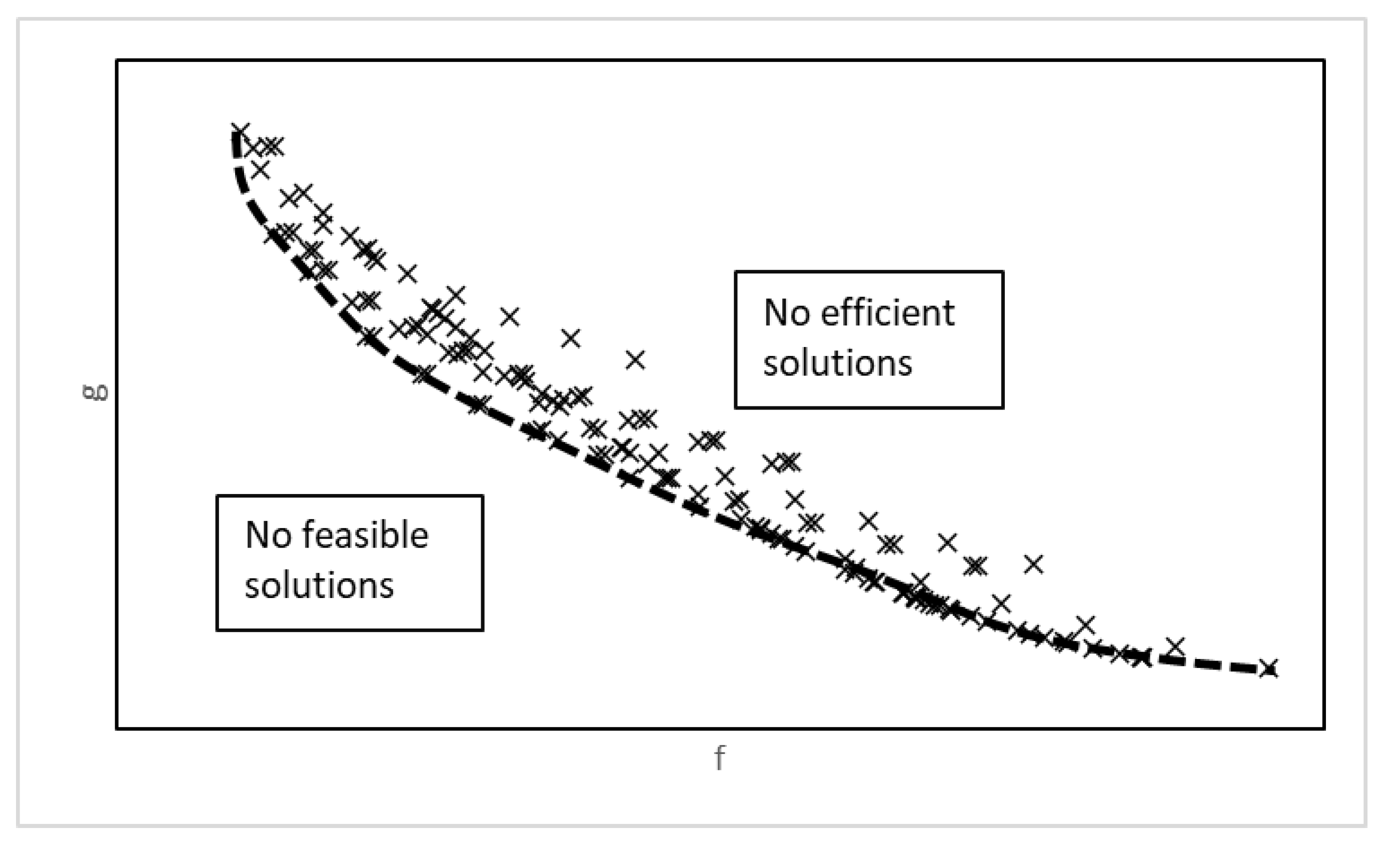
The common solution to the problem of choosing the coefficients is to involve a decision-maker in the process of selecting the most preferable solution. Typically, this is done by first finding the “efficient curve” (i.e., the set of solutions that are optimal for some combination of coefficients). A demonstration of this concept for two objective functions, f and g, is shown in Figure 2. Each plot on this graph is projected into the objective space of a feasible solution, and the efficient curve is shown as a dashed line. No feasible solutions exist below the efficient curve, while solutions above the efficient curve are inefficient. Thus, the efficient curve represents the set of viable and efficient solutions.

This concept is closely related with the concept of the “Pareto front” (i.e., the set of solutions that are Pareto optimal, or non-dominated). The Pareto front includes solutions where there is no feasible solution that is better in all objectives, but it includes a set of solutions with different trade-offs among the conflicting objectives. Selecting between these solutions is done by imposing a set of weighing coefficients. Many methods have been proposed for finding the Pareto front—a subject which is outside the scope of this work. The decision-maker can then analyze the set of solutions and select the most preferable solution. Several tools and methodologies are available to facilitate the decision-making stage; for example, the work presented in [39,40,41,42], and the taxonomy in [43].

While the efficient curve method seems to provide the most freedom to the decision-maker, in our experience, operators find the visualization tools confusing and would rather have clearer operational meaning for their choices.

2.2.2. The E-Constraint Technique

In the e-constraint technique, one of the objective functions to be optimized is selected and the other objectives are considered as constraints by specifying inferior reservation levels that are acceptable in some sense. For target functions $f_1\left(·\right),f_2\left(·\right),\dots ,f_N\left(·\right)$, one target function to be optimized is selected, $f_p\left(·\right)$, and reservation levels $e_i,i\ne p$ are set for the other target functions. The optimization problem is written as

$$\begin{array}{cc}\hfill min& f_p\left(·\right)\hfill \\ \hfill \mathrm{s}.\mathrm{t}.& f_i\left(·\right)\le e_{i}i\ne p\hfill \\ \hfill & \overrightarrow{h}\left(·\right)\le 0.\hfill \end{array}$$

(23)

Note that to achieve strong efficient solutions, $f_p\left(·\right)$ is usually replaced with $f_p\left(·\right)+{\sum }_{i\ne p}{\rho }_i{f}_i\left(·\right)$ with small ${\rho }_i>0$ [26].

It is common practice to first run individual optimizations for each of the target functions and then derive the reservation levels based on the optimal target values. One typical method is to use proportion reservation levels, or percentile reservation levels, through $e_i=(1+{\delta }_i)min{f}_i\left(·\right)$, where ${\delta }_i$ is the reservation proportion for the target function $f_i\left(·\right)$. The advantage of this method is that it has a very clear and intuitive operational interpretation, as follows. If one first sets ${\delta }_i=0$ for $i\ne p$ and derives $min{f}_p\left(·\right)$, then ${\delta }_i$ is the percentile increase of $f_i\left(·\right)$ that one is willing to sacrifice to get a better $f_p\left(·\right)$. For example, if by sacrificing 1% of one target function, another target function is increased by 30%, then this increase is operationally sensible.

Alternatively, $e_i$ can be based on the range as follows: $e_i=min{f}_i\left(·\right)+{\gamma }_i(max{f}_i\left(·\right)-min{f}_i\left(·\right))$, where $0\le {\gamma }_i\le 1,i\ne p$. The operational interpretation of ${\gamma }_i$ is the portion of the range sacrificed. An additive reservation level, $e_i=min{f}_i\left(·\right)+{\mathrm{\Delta }}_i$, may also make operational sense, especially if ${\mathrm{\Delta }}_i$ is in the order of magnitude of the errors in the system.

3. Simulation Results

In this section, the MOO techniques discussed in Section 2.2 are demonstrated by optimizing the active power and reactive power on a test feeder. The test feeder is described, and then each of the methods discussed is demonstrated.

3.1. The Test Feeder

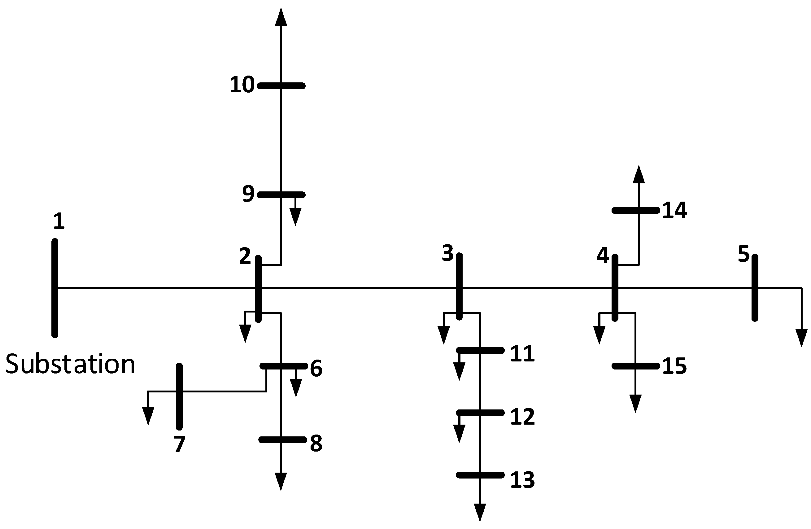
Figure 3 show a single-line diagram of the test feeder, based on [44], with different loads and controls. The feeder is a balanced three-phase $11$ kV rural distribution feeder. The impedances of the lines were taken from [44] without modification and are listed in

Table 1. Loads and impedances of the test feeder.

		Impedance of Line Ending at Bus
Bus #	Load	R ($\mathrm{\Omega }$)	X ($\mathrm{\Omega }$)
1	Slack bus, $0.8$ $\mathrm{MVAr}$
2	$63 \mathrm{kVA},cos\phi =0.7$	1.35309	1.32349
3	$1 \mathrm{k}\mathrm{\Omega }$	1.17024	1.14464
4	$200 \mathrm{k}\mathrm{VA},cos\phi =0.7$	0.84111	0.82271
5	$1 \mathrm{k}\mathrm{\Omega }$	1.52348	1.02760
6	$200 \mathrm{k}\mathrm{VA},cos\phi =0.7$	2.55727	1.72490
7	$1 \mathrm{k}\mathrm{\Omega }$	1.08820	0.73400
8	$100 \mathrm{k}\mathrm{VA},cos\phi =0.7$	1.25143	0.84410
9	$100 \mathrm{k}\mathrm{VA},cos\phi =0.7$	2.01317	1.35790
10	$1 \mathrm{k}\mathrm{\Omega }$	1.68671	1.13770
11	$200 \mathrm{k}\mathrm{VA},cos\phi =0.7$	1.79553	1.21110
12	$1 \mathrm{k}\mathrm{\Omega }$	2.44845	1.65150
13	$63 \mathrm{k}\mathrm{VA},cos\phi =0.7$	2.01317	1.35790
14	$1 \mathrm{k}\mathrm{\Omega }$	2.23081	1.50470
15	$200 \mathrm{k}\mathrm{VA},cos\phi =0.7$	1.19702	0.80740

. The total load is around $2.5$ MW of active power and $0.8$ $\mathrm{M}$$\mathrm{VAr}$ of reactive power. About half of the loads are resistive, and half of the loads work under a constant load and constant power factor regime. In addition, a large $0.8$ $\mathrm{M}$$\mathrm{VAr}$ reactive load is present at bus 1.The exact loads are in listed in Table 1.

The controllable assets are three capacitor banks located at buses 2, 3 and 4 and a solar farm with a controllable inverter located at bus 6. The capacitor banks are on/off switchable rated at 250 $\mathrm{k}$$\mathrm{VAr}$. The solar farm supplies 1 MW with controllable power factor in the interval of $0.8\le cos\phi \le 1$, with increments of 0.02. This provides $2\times 2\times 2\times 11=88$ controllable states. For each controllable state the GridLAB-D software [45] was utilized to calculate the system state.

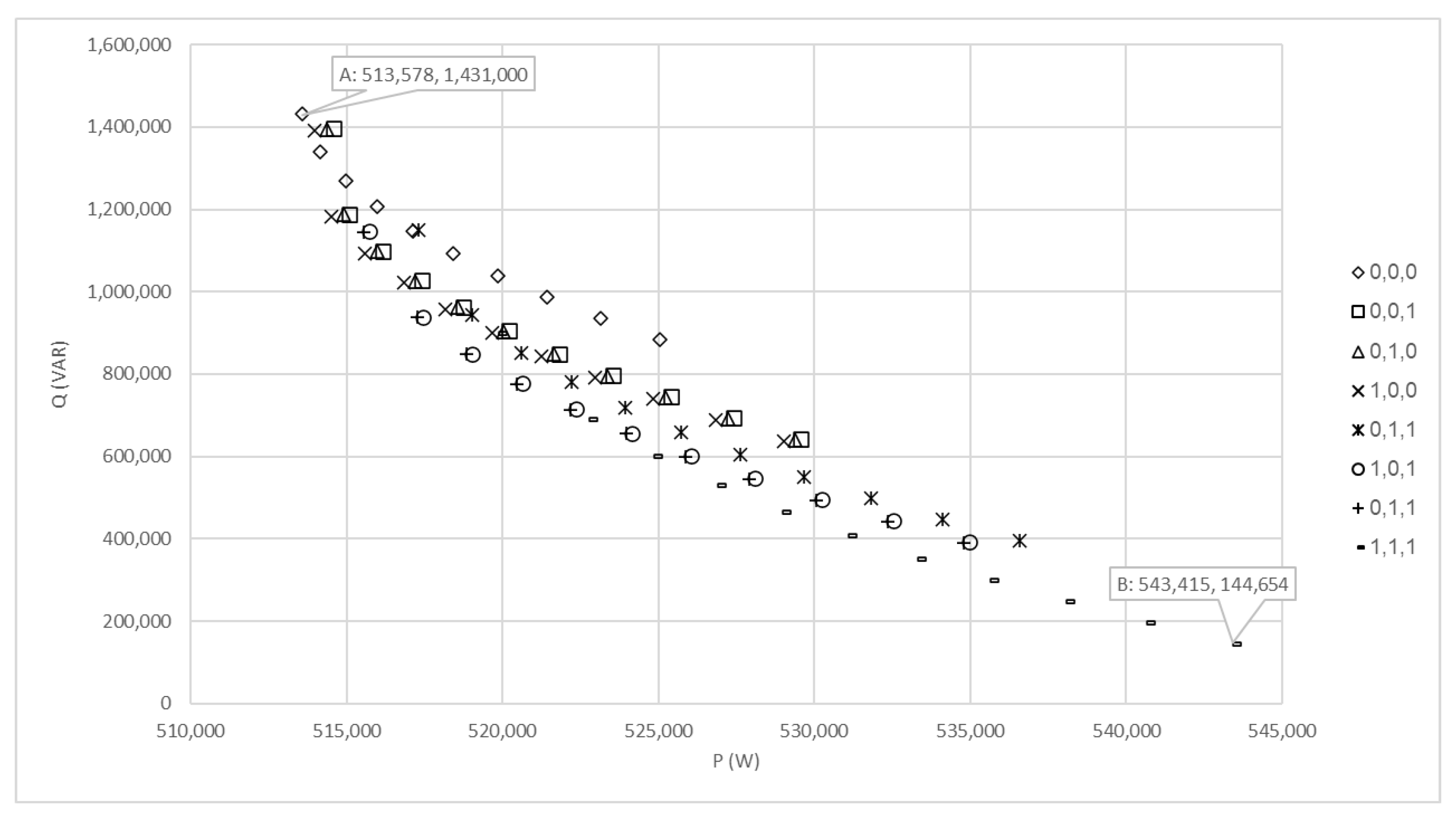
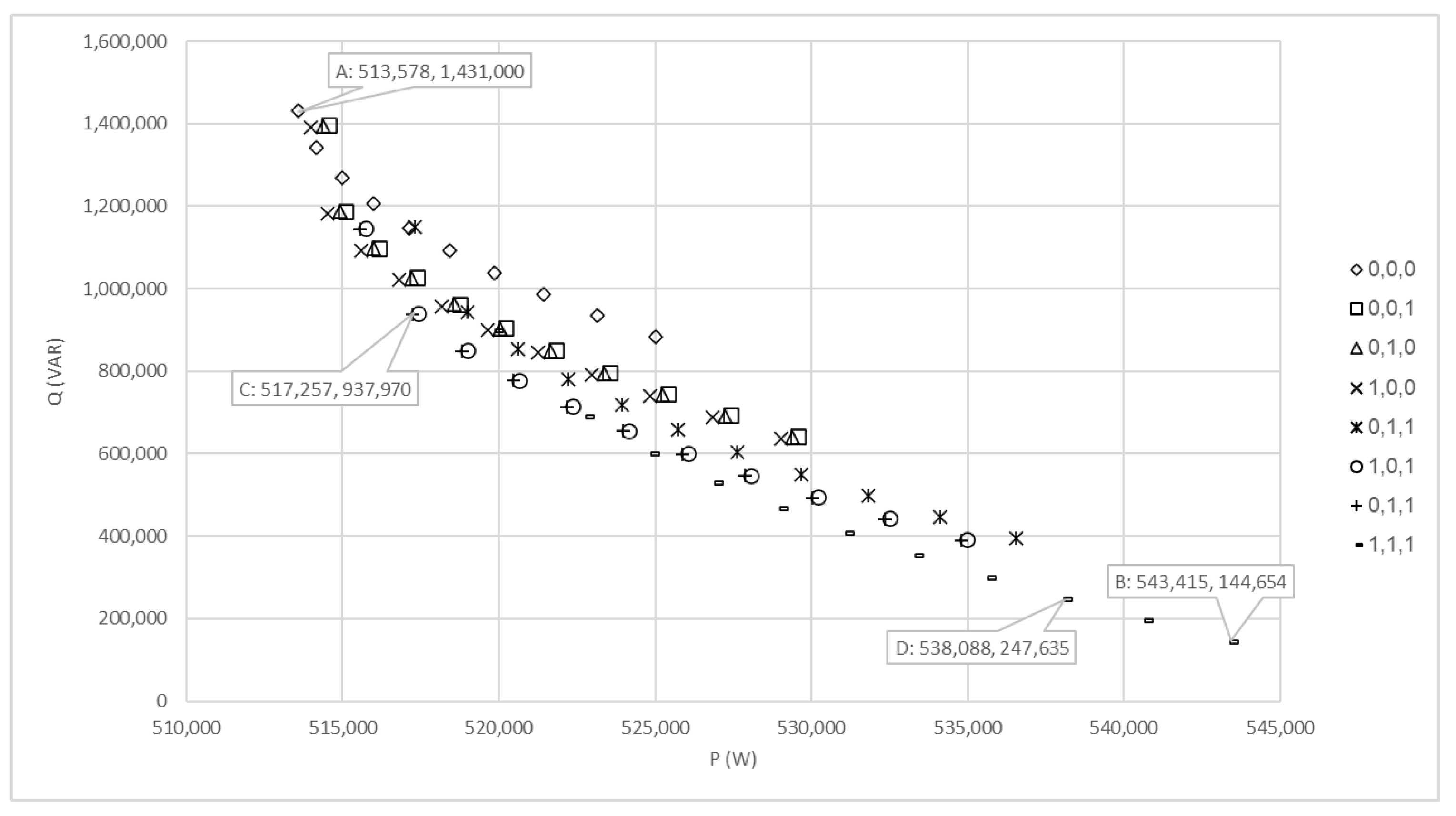
The particulars of the feeder were chosen carefully to demonstrate the trade-off between minimizing the active power at the head bus (Equation (13) $f_p\left(·\right)=P_1$) and minimizing the reactive power at the head bus (Equation (14), $f_q\left(·\right)=Q_1$). Figure 4 shows the calculated active power and reactive power for the 88 controllable states. For each capacitor bank state $X_1,X_2,X_3$, where $X_i=0$ denotes a disconnected capacitor bank and $X_i=1$ denoted a connected capacitor bank, the value of $(P_1,Q_1)$ is plotted for the 11 inverter control points. This clearly demonstrates the trade-off between active power and reactive power, as follows.

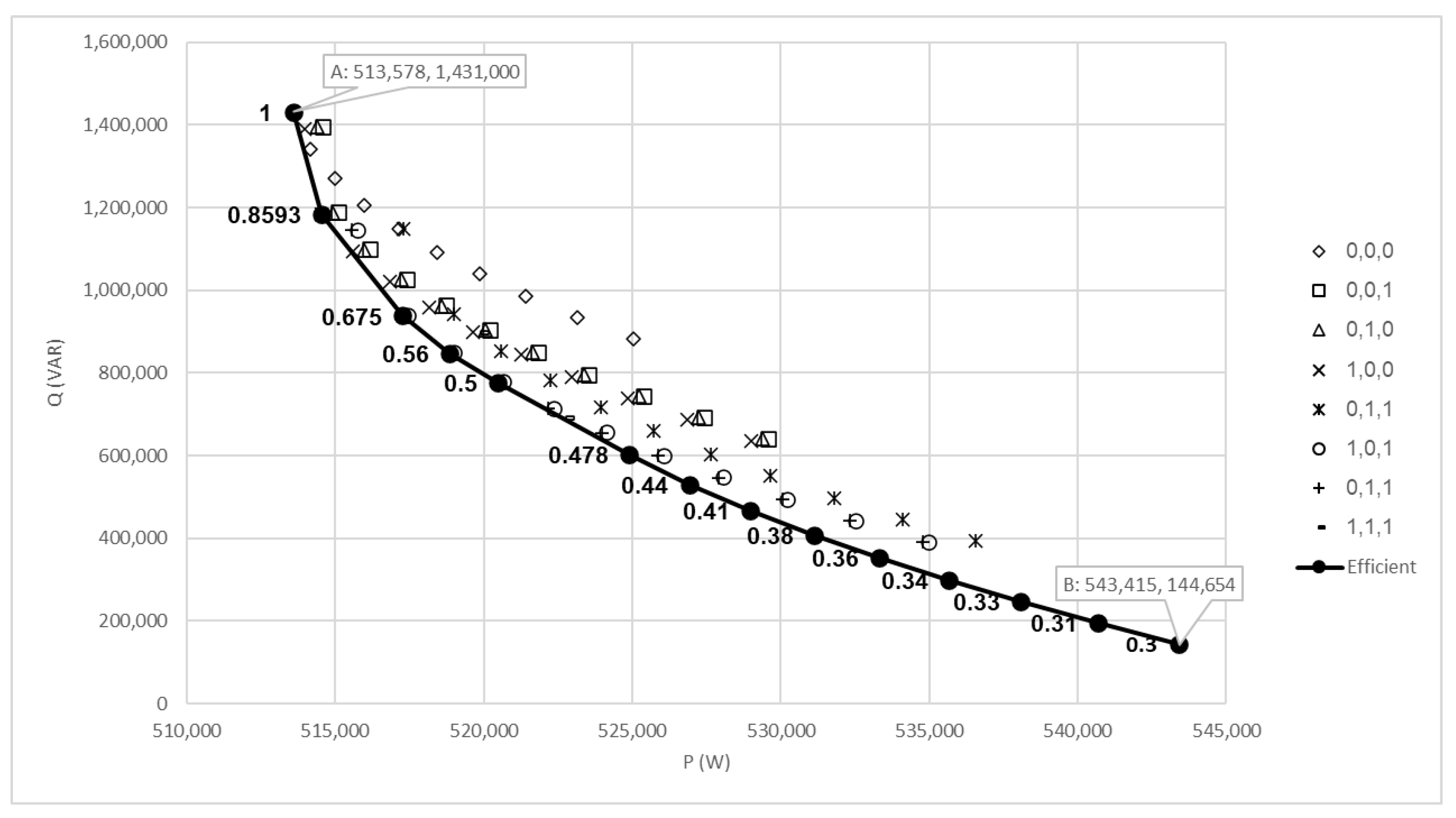
At one extreme, at the P-optimal point, the reactive power is maximized because no capacitor bank is engaged and the solar farm works at $cos\phi =1$. This results in operating point A with $P_{min}\cong 513$ kW and $Q_{P_{min}}\cong 1431\mathrm{k}\mathrm{VAr}$. Engaging capacitor banks and changing $cos\phi$ reduces Q, but it also increases the voltage, which (due to the resistive loads) also increases the active power P. Minimizing Q by engaging all capacitor banks and setting $cos\phi =0.8$ yields operating point B with $Q_{min}\cong 145\mathrm{k}\mathrm{VAr}$ and $P_{Q_{min}}\cong 543$ kW.

3.2. Applying the Weighted-Sum Technique for Active and Reactive Power Optimization

The weighted-sum technique with the $\alpha :(1-\alpha )$ method was applied to the feeder. Both active power and reactive power were normalized, and efficient points for every value of $\alpha$ were calculated. The resulting efficient frontier is shown in Figure 5. Of the possible 88 operating points, 14 operating points belong to the efficient curve. The maximum value of $\alpha$ corresponding to each point is also shown.

In a practical setting, these 14 possible control points are shown to the decision-maker and a choice is then made. While this provides the decision-maker with the most operational freedom, it does not provide an intuitive operational interpretation of the decision other than that it is “efficient”.

3.3. Applying the E-Constraint Technique for Active and Reactive Power Optimization

The e-constraint technique was applied to the feeder, and the results are shown in Figure 6.

To begin with, Q was optimized with a reservation level on P as a constraint. The percentile reservation level was used, setting ${\delta }_P=1\%$, which yielded the reservation level $e_P=519$ kW. This led to the optimal operating point C, where capacitors banks 2 and 3 were engaged and $cos\phi =0.98$. This yielded $P_C\cong 517$ kW and $Q_C\cong 938\mathrm{k}\mathrm{VAr}$. The operational interpretation is very clear: for a loss of optimality of 1% in active power, $938\mathrm{k}\mathrm{VAr}$ is gained, which is a gain of 34%. Alternatively, this can be seen as an additive reservation level, where ${\Delta }_P=5$ kW. The interpretation of this would be a gain of $938\mathrm{k}\mathrm{VAr}$ for a loss of 5.

To optimize P with a reservation level on Q as constraint, a range reservation level was used. Selecting $\gamma =10\%$ yielded the reservation level $e_Q=273\mathrm{k}\mathrm{VAr}$. Optimizing for P led to the optimal operating point D, where all capacitors banks were engaged and $cos\phi =0.84$. This yielded $P_D\cong 538$ kW and $Q_D\cong 247\mathrm{k}\mathrm{VAr}$. Operationally speaking, for a loss of 10% of the range in Q, the gain is $5$ kW, which is 18% of the range of P.

4. Discussion and Conclusions

In this work, an operational approach to multi-objective optimization for Volt-VAr cCntrol was investigated. A general formulation of this multi-objective problem was presented by first defining a general single-objection optimization method, including time and scenario-based optimization, and then extending it to the multi-objective case.

In this context, two general techniques for multi-objective optimization were discussed, namely the weighted-sum technique, which is often combined with an efficient/Pareto optimal curve, and the e-constraint technique, which can be used with various reservation level-setting methods. The operational interpretation of the solutions achieved by these techniques was discussed. Both techniques were demonstrated with a simulation on a test feeder. The results clearly demonstrate that a trade-off can exist between multiple objectives. For the weighted-sum technique, the simulation demonstrated the existence of an efficient curve and showed how a choice can be presented to the decision-maker. For the e-constraint technique, the simulation showed how solutions with a clear operational interpretation can be achieved by using intuitive reservation level-setting methods.

This work has both theoretical and practical impacts. The main theoretical impact is that the work provides a theoretical framework for expressing multi-objective problems in the field of Volt-VAr control. The framework can ease and simplify the communication between researchers. The major practical impact of this work is that distribution system operators, and other practitioners, can use the proposed simple multi-objective optimization techniques to operate distribution systems in a manner which optimizes more than one target function; for example, optimizing both active power and reactive power. In addition, the discussion of the operational interpretation of multi-objective optimization, which was lacking in the research, may further facilitate the adoption of these multi-objective techniques in Volt-VAr applications and other control operations in distribution systems, especially when the operational interpretations are intuitive.

It is worth mentioning that there are of course many other techniques for multi-objective optimization. For example, variants of fuzzy compromise functions are used in [31,33]. The aim of this work was not to review every technique in this area. Instead, the aim was to focus on the most widely used techniques, and especially those that may yield to operational interpretation. In a field that is little researched but which seems to have vast operational benefits, the fundamentals provided, and especially the intuitive operational interpretation, may facilitate the faster adoption of multi-objective Volt-VAr Optimization solutions.

References

- Masetti, C. Revision of European Standard EN 50160 on power quality: Reasons and solutions. In Proceedings of the 14th International Conference on Harmonics and Quality of Power—ICHQP 2010, Bergamo, Italy, 26–29 September 2010; pp. 1–7. [Google Scholar]
- Yang, Y.; Enjeti, P.; Blaabjerg, F.; Wang, H. Wide-Scale Adoption of Photovoltaic Energy: Grid Code Modifications Are Explored in the Distribution Grid. IEEE Ind. Appl. Mag. 2015, 21, 21–31. [Google Scholar] [CrossRef] [Green Version]
- Kundur, P.; Balu, N.; Lauby, M. Power System Stability and Control; EPRI Power System Engineering Series; McGraw-Hill Education: New York, NY, USA, 1994. [Google Scholar]
- Hashim, T.T.; Mohamed, A.; Shareef, H. A review on voltage control methods for active distribution networks. Prz. Elektrotechniczny (Electr. Rev.) 2012, 88, 304–312. [Google Scholar]
- Carvallo, A.; Cooper, J. The Advanced Smart Grid: Edge Power Driving Sustainability; Artech House: Boston, MA, USA, 2015. [Google Scholar]
- Borozan, V.; Baran, M.E.; Novosel, D. Integrated Volt/VAr control in distribution systems. In Proceedings of the 2001 IEEE Power Engineering Society Winter Meeting, Conference Proceedings (Cat. No.01CH37194). Columbus, OH, USA, 28 January–1 February 2001; Volume 3, pp. 1485–1490. [Google Scholar]
- Liu, Y.; Zhang, P.; Qiu, X. Optimal volt/var control in distribution systems. Int. J. Electr. Power Energy Syst. 2002, 24, 271–276. [Google Scholar] [CrossRef]
- Niknam, T.; Nayeripour, M.; Olamaei, J.; Arefi, A. An efficient hybrid evolutionary optimization algorithm for daily Volt/Var control at distribution system including DGs. Int. Rev. Electr. Eng. 2008, 3, 513–524. [Google Scholar]
- Tomin, N.; Kurbatsky, V.; Panasetsky, D.; Sidorov, D.; Zhukov, A. Voltage/VAR Control and Optimization: AI approach. IFAC-PapersOnLine 2018, 51, 103–108. [Google Scholar] [CrossRef]
- Ma, H.M.; Man, K.F.; Hill, D.J. Control strategy for multi-objective coordinate voltage control using hierarchical genetic algorithms. In Proceedings of the 2005 IEEE International Conference on Industrial Technology, Hong Kong, China, 14–17 December 2005; pp. 158–163. [Google Scholar]
- Lemos, F.A.; Feijó, W.L., Jr.; Werberich, L.C.; Rosa, M. Assessment of a sub-transmission and distribution system under coordinated secondary voltage control. In Proceedings of the 14th PSCC-Power System Computational Conference, Seville, Spain, 24–28 June 2002. [Google Scholar]
- Kim, G.W.; Lee, K.Y. Coordination control of ULTC transformer and STATCOM based on an artificial neural network. IEEE Trans. Power Syst. 2005, 20, 580–586. [Google Scholar] [CrossRef]
- Le, A.D.; Muttaqi, K.M.; Negnevitsky, M.; Ledwich, G. Response coordination of distributed generation and tap changers for voltage support. In Proceedings of the 2007 Australasian Universities Power Engineering Conference, Perth, WA, Australia, 9–12 December 2007; pp. 1–7. [Google Scholar]
- Arshad, A.; Lehtonen, M. Multi-agent system based distributed voltage control in medium voltage distribution systems. In Proceedings of the 2016 17th International Scientific Conference on Electric Power Engineering (EPE), Prague, Czech Republic, 16–18 May 2016; pp. 1–6. [Google Scholar] [CrossRef]
- Raz, D.; Daliot, A. Generalized approach for Volt-VAr-Control through integration of DERs with traditional methods. Grid Future Symp. 2018, 2018, article 55. [Google Scholar]
- Geoffrion, A.M. Solving bicriterion mathematical programs. Oper. Res. 1967, 15, 39–54. [Google Scholar] [CrossRef]
- Gandibleux, X. Multiple Criteria Optimization: State of the Art Annotated Bibliographic Surveys; International Series in Operations Research & Management Science; Springer Science & Business Media: Boston, MA, USA, 2006; Volume 52. [Google Scholar]
- Deb, K. Multi-objective optimization. In Search Methodologies; Springer: Boston, MA, USA, 2014; pp. 403–449. [Google Scholar]
- Jones, D.; Mirrazavi, S.; Tamiz, M. Multi-objective meta-heuristics: An overview of the current state-of-the-art. Eur. J. Oper. Res. 2002, 137, 1–9. [Google Scholar] [CrossRef]
- Coello Coello, C.A. Evolutionary multi-objective optimization: A historical view of the field. IEEE Comput. Intell. Mag. 2006, 1, 28–36. [Google Scholar] [CrossRef]
- Zhou, A.; Qu, B.Y.; Li, H.; Zhao, S.Z.; Suganthan, P.N.; Zhang, Q. Multiobjective evolutionary algorithms: A survey of the state of the art. Swarm Evol. Comput. 2011, 1, 32–49. [Google Scholar] [CrossRef]
- Miguel Antonio, L.; Coello Coello, C.A. Coevolutionary Multiobjective Evolutionary Algorithms: Survey of the State-of-the-Art. IEEE Trans. Evol. Comput. 2018, 22, 851–865. [Google Scholar] [CrossRef]
- Liu, Q.; Li, X.; Liu, H.; Guo, Z. Multi-objective metaheuristics for discrete optimization problems: A review of the state-of-the-art. Appl. Soft Comput. 2020, 93, 106382. [Google Scholar] [CrossRef]
- Zeleny, M. Linear Multiobjective Programming; Lecture Notes in Economics and Mathematical Systems; Springer: Berlin/Heidelberg, Germany, 1974; Volume 95. [Google Scholar]
- Deb, K. Multi-Objective Optimization Using Evolutionary Algorithms; John Wiley & Sons: Chichester, NY, USA, 2001; Volume 16. [Google Scholar]
- Antunes, C.H.; Alves, M.J.; Climaco, J. Multiobjective Linear and Integer Programming; Springer: Boston, MA, USA, 2016. [Google Scholar]
- Alarcon-Rodriguez, A.; Ault, G.; Galloway, S. Multi-objective planning of distributed energy resources: A review of the state-of-the-art. Renew. Sustain. Energy Rev. 2010, 14, 1353–1366. [Google Scholar] [CrossRef]
- Fadaee, M.; Radzi, M. Multi-objective optimization of a stand-alone hybrid renewable energy system by using evolutionary algorithms: A review. Renew. Sustain. Energy Rev. 2012, 16, 3364–3369. [Google Scholar] [CrossRef]
- Turitsyn, K.; Sulc, P.; Backhaus, S.; Chertkov, M. Options for Control of Reactive Power by Distributed Photovoltaic Generators. Proc. IEEE 2011, 99, 1063–1073. [Google Scholar] [CrossRef] [Green Version]
- Wang, Z.; Wang, J.; Chen, B.; Begovic, M.M.; He, Y. MPC-Based Voltage/Var Optimization for Distribution Circuits With Distributed Generators and Exponential Load Models. IEEE Trans. Smart Grid 2014, 5, 2412–2420. [Google Scholar] [CrossRef]
- Niknam, T.; Zare, M.; Aghaei, J. Scenario-Based Multiobjective Volt/Var Control in Distribution Networks Including Renewable Energy Sources. IEEE Trans. Power Deliv. 2012, 27, 2004–2019. [Google Scholar] [CrossRef]
- Zhang, C.; Dong, Z.; Xu, Y. Multi-Objective Robust Voltage/VAR Control for Active Distribution Networks. In Proceedings of the 2019 IEEE Power Energy Society General Meeting (PESGM), Atlanta, GA, USA, 4–8 August 2019; pp. 1–5. [Google Scholar]
- Hou, J.; Xu, Y.; Liu, J.; Xin, L.; Wei, W. A multi-objective volt-var control strategy for distribution networks with high PV penetration. In Proceedings of the 10th International Conference on Advances in Power System Control, Operation Management (APSCOM 2015), Hong Kong, China, 8–12 November 2015; pp. 1–6. [Google Scholar]
- Auchariyamet, S.; Sirisumrannukul, S. Volt/VAr control in distribution systems by fuzzy multiobjective and particle swarm. In Proceedings of the 2009 6th International Conference on Electrical Engineering/Electronics, Computer, Telecommunications and Information Technology, Pattaya, Chonburi, Thailand, 6–9 May 2009; Volume 1, pp. 234–237. [Google Scholar] [CrossRef] [Green Version]
- Castro, J.R.; Saad, M.; Lefebvre, S.; Asber, D.; Lenoir, L. Coordinated voltage control in distribution network with the presence of DGs and variable loads using pareto and fuzzy logic. Energies 2016, 9, 107. [Google Scholar] [CrossRef] [Green Version]
- Saravanakathir, B.; Sasiraja, R. Optimal Coordinated Voltage Control Method for Distribution Network in Presence of Distributed Generators. Int. J. Eng. Sci 2017, 7, 12117–12122. [Google Scholar]
- Zare, M.; Niknam, T.; Azizipanah-Abarghooee, R.; Amiri, B. Multi-objective probabilistic reactive power and voltage control with wind site correlations. Energy 2014, 66, 810–822. [Google Scholar] [CrossRef]
- Wang, P.; Deng, X.; Zhou, H.; Yu, S. Estimates of the social cost of carbon: A review based on meta-analysis. J. Clean. Prod. 2019, 209, 1494–1507. [Google Scholar] [CrossRef]
- Blasco, X.; Herrero, J.M.; Sanchis, J.; Martínez, M. A new graphical visualization of n-dimensional Pareto front for decision-making in multiobjective optimization. Inf. Sci. 2008, 178, 3908–3924. [Google Scholar] [CrossRef]
- Cela, R.; Bollaín, M. New cluster mapping tools for the graphical assessment of non-dominated solutions in multi-objective optimization. Chemom. Intell. Lab. Syst. 2012, 114, 72–86. [Google Scholar] [CrossRef]
- de Freitas, A.R.; Fleming, P.J.; Guimarães, F.G. Aggregation trees for visualization and dimension reduction in many-objective optimization. Inf. Sci. 2015, 298, 288–314. [Google Scholar] [CrossRef] [Green Version]
- Tušar, T.; Filipič, B. Visualization of Pareto front approximations in evolutionary multiobjective optimization: A critical review and the prosection method. IEEE Trans. Evol. Comput. 2014, 19, 225–245. [Google Scholar] [CrossRef]
- Reynoso-Meza, G.; Blasco, X.; Sanchis, J.; Herrero, J.M. Comparison of design concepts in multi-criteria decision-making using level diagrams. Inf. Sci. 2013, 221, 124–141. [Google Scholar] [CrossRef] [Green Version]
- Das, D.; Kothari, D.; Kalam, A. Simple and efficient method for load flow solution of radial distribution networks. Int. J. Electr. Power Energy Syst. 1995, 17, 335–346. [Google Scholar] [CrossRef]
- Chassin, D.P.; Schneider, K.; Gerkensmeyer, C. GridLAB-D: An open-source power systems modeling and simulation environment. In Proceedings of the 2008 IEEE/PES Transmission and Distribution Conference and Exposition, Bogota, CO, USA, 13–15 August 2008; pp. 1–5. [Google Scholar]
Figure 1.
An illustration of the proposed multi-objective optimization–Volt-VAr Control (MMO–VVC) approach. Data are presented in parallelograms and functions are presented in rectangles.
Figure 2.
Efficient curve example. Each plot is a feasible solution; the efficient curve is shown as a dashed line.
Figure 3.
Modified single-line diagram of the test feeder, based on [44].
Figure 4.
Calculated active power (P, in ) and reactive power (Q, in ) for all control points in the test feeder, with highlighted extreme points.
Figure 5.
Calculated active power (P, in ) and reactive power (Q, in ) on the test feeder, with the efficient curve highlighted and values.
Figure 6.
Calculated active power (P, in ) and reactive power (Q, in ) for all control points in the test feeder, with highlighted points of interest.