Acoustic Emission Characteristics and Joint Nonlinear Mechanical Response of Rock Masses under Uniaxial Compression


1
State Key Laboratory for Geomechanics & Deep Underground Engineering, China University of Mining and Technology (Beijing), Beijing 100083, China
2
School of Mechanics and Civil Engineering, China University of Mining and Technology (Beijing), Beijing 100083, China
*
Author to whom correspondence should be addressed.
Energies 2021, 14(1), 200; https://doi.org/10.3390/en14010200
Submission received: 28 November 2020
/
Revised: 26 December 2020
/
Accepted: 29 December 2020
/
Published: 2 January 2021
(This article belongs to the Special Issue Sustainable Geotechnical Engineering and Its Applications)
Abstract
:The joint arrangement in rock masses is the critical factor controlling the stability of rock structures in underground geotechnical engineering. In this study, the influence of the joint inclination angle on the mechanical behavior of jointed rock masses under uniaxial compression was investigated. Physical model laboratory experiments were conducted on jointed specimens with a single pre-existing flaw inclined at 0°, 30°, 45°, 60°, and 90° and on intact specimens. The acoustic emission (AE) signals were monitored during the loading process, which revealed that there is a correlation between the AE characteristics and the failure modes of the jointed specimens with different inclination angles. In addition, particle flow code (PFC) modeling was carried out to reproduce the phenomena observed in the physical experiments. According to the numerical results, the AE phenomenon was basically the same as that observed in the physical experiments. The response of the pre-existing joint mainly involved three stages: (I) the closing of the joint; (II) the strength mobilization of the joint; and (III) the reopening of the joint. Moreover, the response of the pre-existing joint was closely related to the joint’s inclination. As the joint inclination angle increased, the strength mobilization stage of the joint gradually shifted from the pre-peak stage of the stress–strain curve to the post-peak stage. In addition, the instantaneous drop in the average joint system aperture () in the specimens with medium and high inclination angles corresponded to a rapid increase in the form of the pulse of the AE activity during the strength mobilization stage.
1. Introduction
The damage development of underground caverns and rock slopes during the excavation processes and the activities of large underground faults may trigger microseismic events and earthquakes, respectively [1]. The propagation of the original internal cracks and defects within the rock and the initiation, propagation and coalescence of new microcracks release elastic waves during the damage process, which are called acoustic emissions (AEs) [2]. In the 1930s, Obert [3] first applied AE technology to the monitoring and prediction of the stability of mine pillars and rock bursts. Since then, AE technology has been extensively used in geotechnical engineering. Based on the AE characteristics of the rock failure process, several researchers have conducted extensive laboratory research on the AE characteristics of rocks under compression [4,5,6], tension [7], shear [8], and fracture test conditions [9]. Mogi [10] conducted a large number of AE experiments on rocks and explored the AE characteristics of the rock fracture process under pressure. Holcomb and Costin [11] used the Kaiser effect—that is, that the onset of AE indicates the initiation of damage—to establish a connection between the AE and the damaged surfaces. Subsequently, Pestman and Munster [12] used the Kaiser effect to study the relationship between the AE characteristics of sandstone and the shape of the damaged surfaces under triaxial stress.
As the variability of the AE signal parameters is affected by various static and dynamic factors, such as the material properties, deformation characteristics, and damage evolution of the specimen, and these factors also influence each other, it is difficult to extract the effective AE characteristics, which affects the theoretical and experimental research of AE signals. Thus, several researchers have attempted to use numerical modeling of AEs to further improve and supplement their experimental and theoretical results [13,14,15]. Hazzard and Young [16] studied the theory of the AE numerical simulation algorithm using the particle flow code (PFC2D), and they further demonstrated the feasibility of using bond breakage to simulate AEs. Then, they extended this algorithm to PFC3D [17], and the model produced seismic events with realistic locations, magnitudes, and mechanisms. Su et al. [18] used PFC2D to simulate the AEs of rock samples with different degrees of heterogeneity, and the breakage of a bond between two particles was regarded as an AE signal. The AE event of a rock can be simulated by counting the number of bond breakages (or microcracks), and the results have shown that the maximum value of the AE lags behind the peak strength. Moreover, as the heterogeneity of the rock increases, the hysteresis effect of the AE signals becomes significant. Wang et al. [19] also regarded the breaking of a bond in a sample as an AE; they compared it with the AE rate obtained from physical model tests in order to calibrate the PFC2D model. Cai et al. [20] used the FLAC/PFC coupling numerical method to study the AE of the Kannagawa underground powerhouse cavern in Japan, and they successfully applied AE simulations at the engineering scale.
AE signals can reflect the characteristics of rock damage, but they are difficult to observe, and it is difficult to comprehensively evaluate the opened/closed state of a pre-existing joint and the detailed process of the pre-existing joint mobilization using AE [21]. Thus, various numerical methods have been extensively used to study the influence of pre-existing joints on the damage mechanism of a rock mass, such as the finite element method (FEM) [22,23,24], the boundary element method (BEM) [25], and the discrete element method (DEM) [26,27,28]. In recent years, the particle flow code (PFC), which was developed based on the DEM, has been extensively used to study the damage mechanism of rock masses [29,30]. Sagong et al. [31] simulated the rock fracture and joint sliding of jointed rock masses with an opening under biaxial compression and investigated the dependence of the damage zone around the hole on the different joint inclination angles. Cheng et al. [32] used PFC2D to perform uniaxial compression tests on nonpersistent jointed rock masses and found that the strength mobilization of the joint system plays a crucial role in strain-softening behaviors. Subsequently, Chen et al. [33] built upon this research and found that the strain-softening behavior was mainly determined by the interactions between the joints, rock bridges, and matrix. Moreover, Shang used PFC3D modeling to simulate the rupture of veined granite under polyaxial compression [34].
In the above-described laboratory tests and numerical modeling, few of the studies analyzed the influence of pre-existing flaws on the failure mechanism of specimens using this research method, that is, combining physical experiments with AE monitoring and numerical simulations from microscopic perspectives. In this study, we combined AE parameters obtained from laboratory tests with the number of crack elements in the numerical model to analyze the damage mechanism of rock masses. In addition, the relationship between the response of a pre-existing joint and the AE characteristic was analyzed.
2. Introduction to Laboratory Tests
2.1. Specimen Preparation and Mechanical Properties of Materials
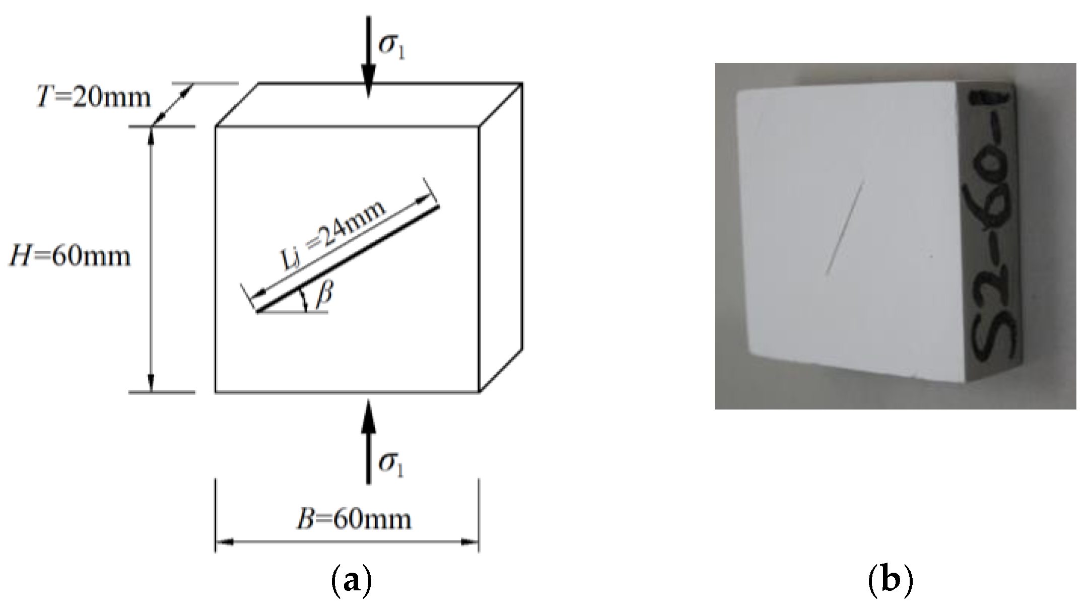
Since a natural rock contains a large number of random cracks, it is difficult to quantitatively analyze the influence of the joint inclination angles on the mechanical behaviors of a rock in the laboratory. Hence, gypsum specimens were used in this experiment. The geometry of the specimen and a photograph of a sample are presented in Figure 1. The dimensions of the specimens were 60 × 60 × 20 mm3 in width, length, and thickness, respectively. A single joint penetrated completely through the specimen. The joint inclination angles (β) inside the different specimens were 0°, 30°, 45°, 60°, and 90°, and the length and thickness of the joint were fixed at = 24 mm and 0.4 mm, respectively. The artificial joints in the specimens were created by inserting steel sheets into the uncured mixture. The partially cured mixture was stored at room temperature for 21 days before the uniaxial compression tests were performed. In order to eliminate testing errors, at least three of each type of specimen were prepared. The uniaxial compressive strength (UCS), Poisson’s ratio (v), and Young’s modulus (E) were measured during the uniaxial compression test of a standard cylindrical specimen (50 mm in diameter and 100 mm in length). The cohesion (c) and internal friction angle (φ) were measured during the standard triaxial compression test of standard cylindrical specimen. The physical and mechanical properties of the intact specimen are presented in Table 1.
2.2. Experimental Setup and Conditions
The pressure in the uniaxial compression experiments was provided using a servo-controlled Changchun Machinery SLB100 test machine. The displacement control mode with a constant loading rate of 0.003 mm/s was used for the experiments. High-definition digital cameras and video cameras were used to record the failure process of the specimen’s surface. A PCI-2 AE system (Physical Acoustic Corporation, Princeton, NJ, USA) was used to collect, store, and analyze the AE signal in real-time.
The AE system consisted of transducers, preamplifiers, and a data acquisition system. Four transducers were placed on the surface of each specimen. To ensure a good contact with the sample, the sensor was fixed in place using an electromagnetic fixture, and a couplant was applied to the contact between the sample and the sensor (Figure 2). The signals were amplified by 40 dB using a preamplifier. The resonant frequency of the AE transducer was 300 kHz, and the AE threshold was 45 dB. An event was defined as a local deformation of the material identified by one or several hits.
2.3. AE Parameter Selection
Using a series of basic AE parameters to characterize the AE signal is the most common way to record an AE event. These parameters include the hits, amplitude, energy, duration, and rise time. In this experiment, the number of hits per second (HPS) on all of the channels was counted [35], and the statistical parameters HPS and energy were used to evaluate the AE activity.
3. Experimental Results
3.1. AE Sequential Characteristics and Failure Modes
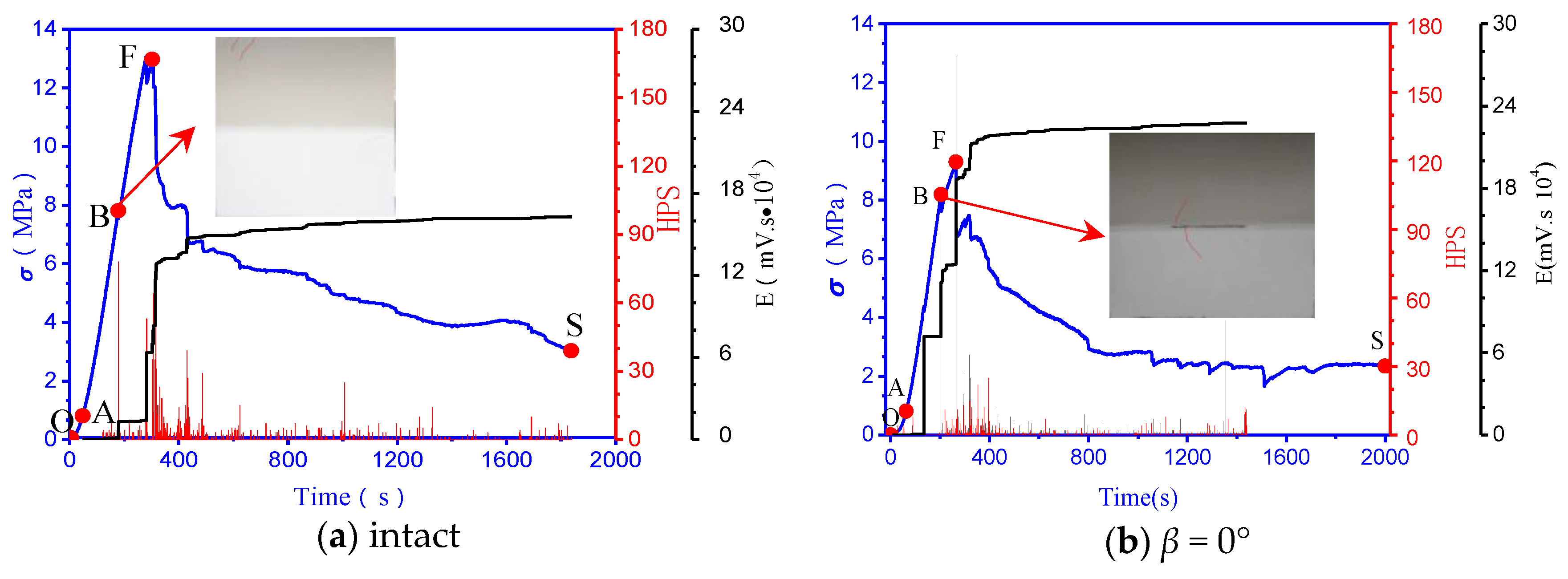
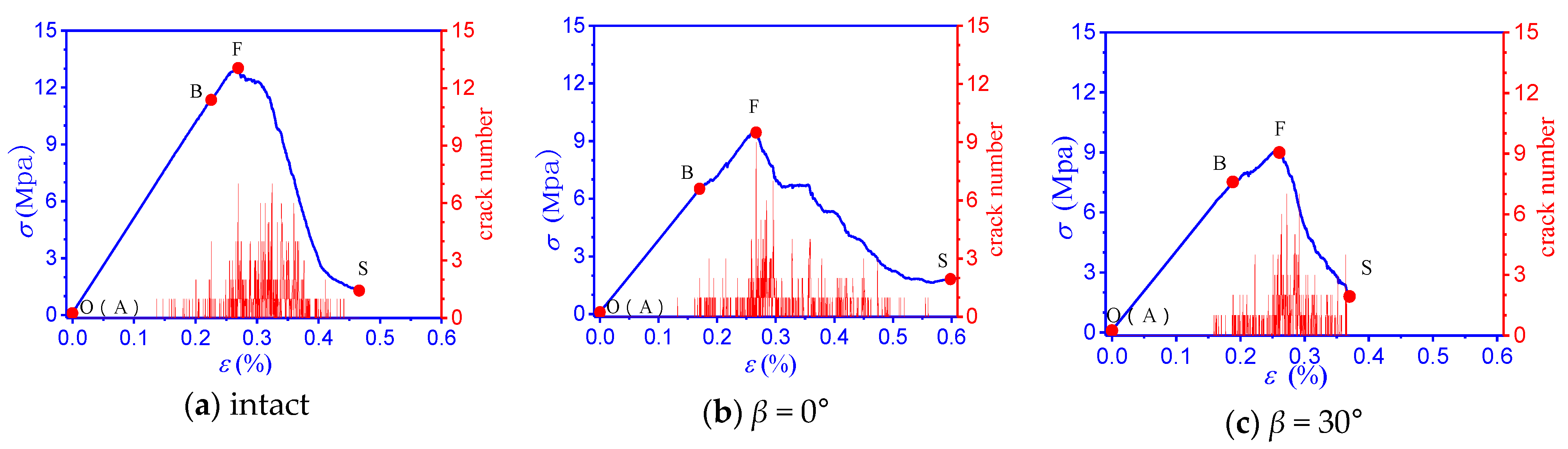
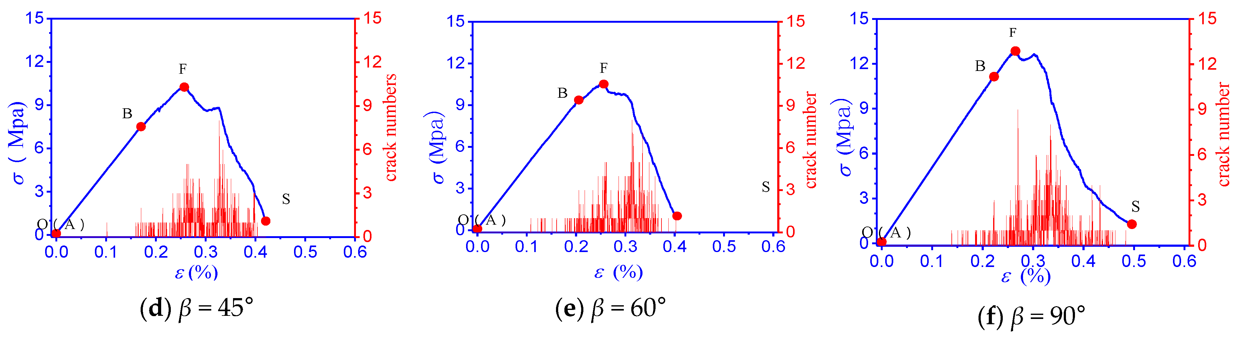
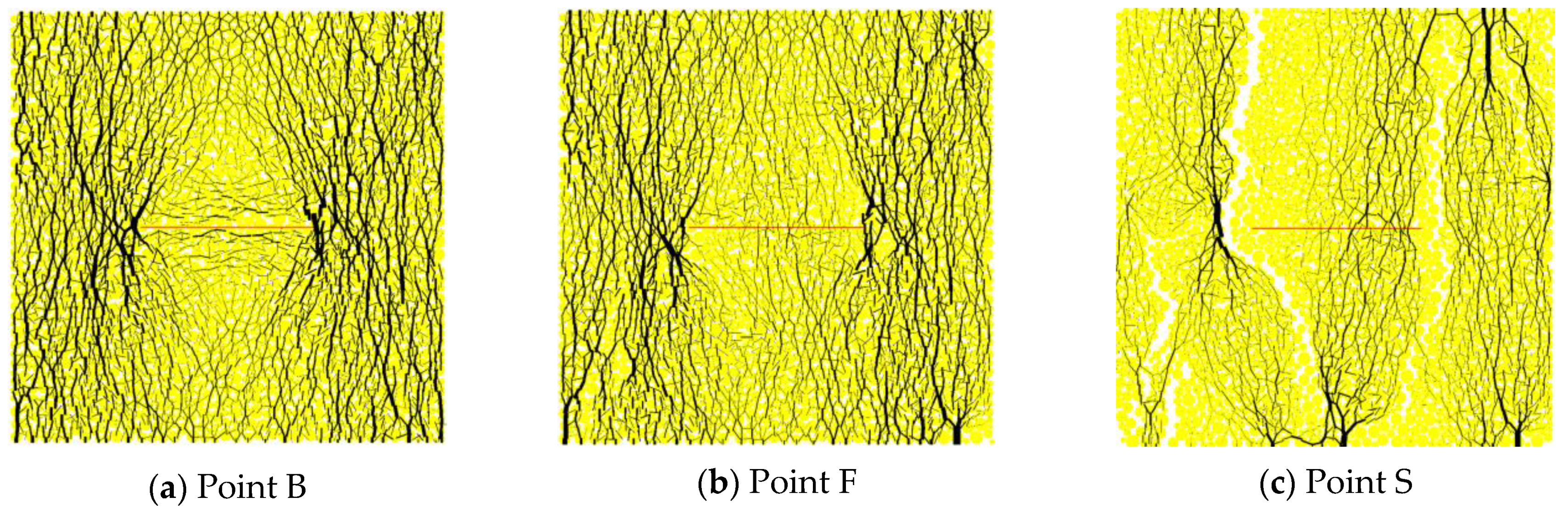
The variations in the stress, HPS, and energy accumulation over time are shown in Figure 3. The deformation characteristics were almost the same for all of the specimens under uniaxial compression. The definitions of the characteristic points on the stress–strain curve are given in Table 2. All of the stress–strain curves can be divided into the following four stages: the initial compaction stage (OA), the elastic deformation stage (AB), the plastic deformation stage (BF), and the post-peak failure stage (FS). It should be noted that point B on the stress–strain curve was selected when the cracks on the surface of the specimens suddenly initiate (Figure 3). The HPS and energy accumulation correspond well to the four stages of the loading process.
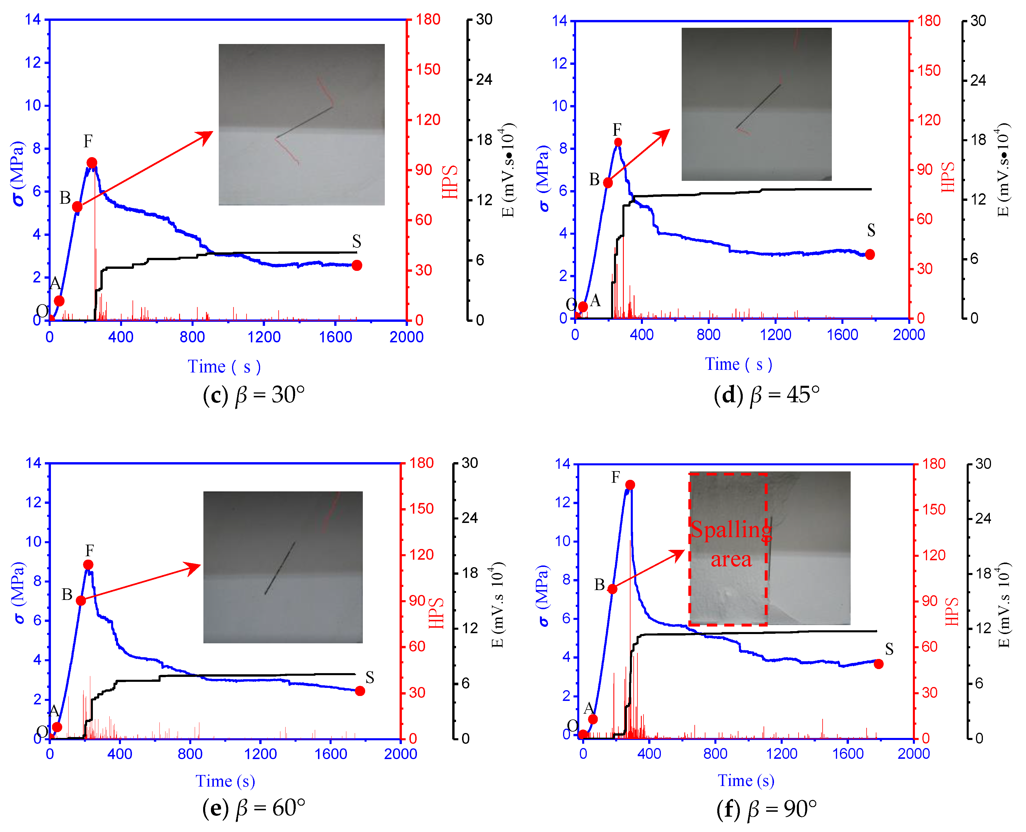
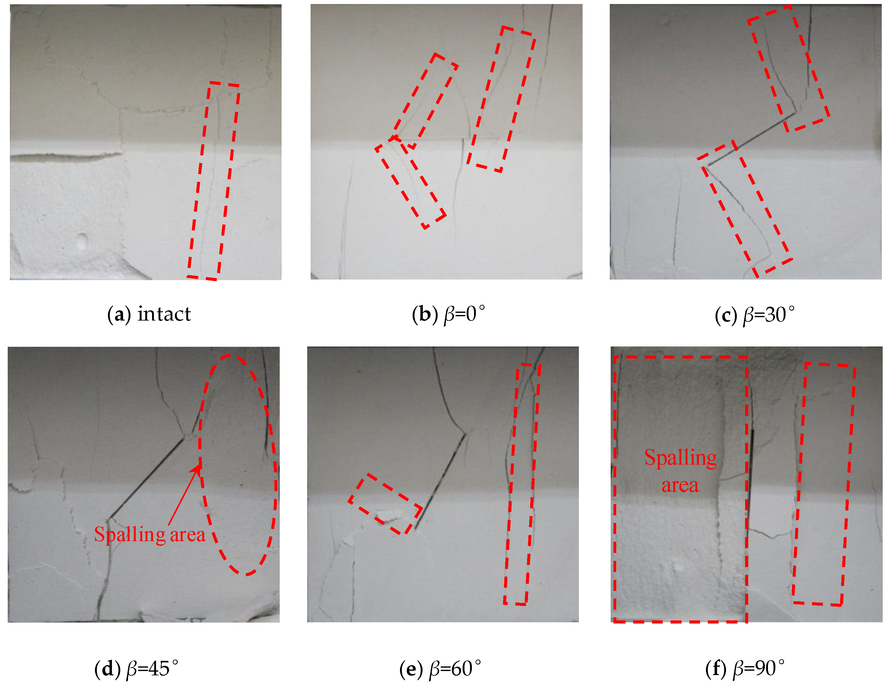
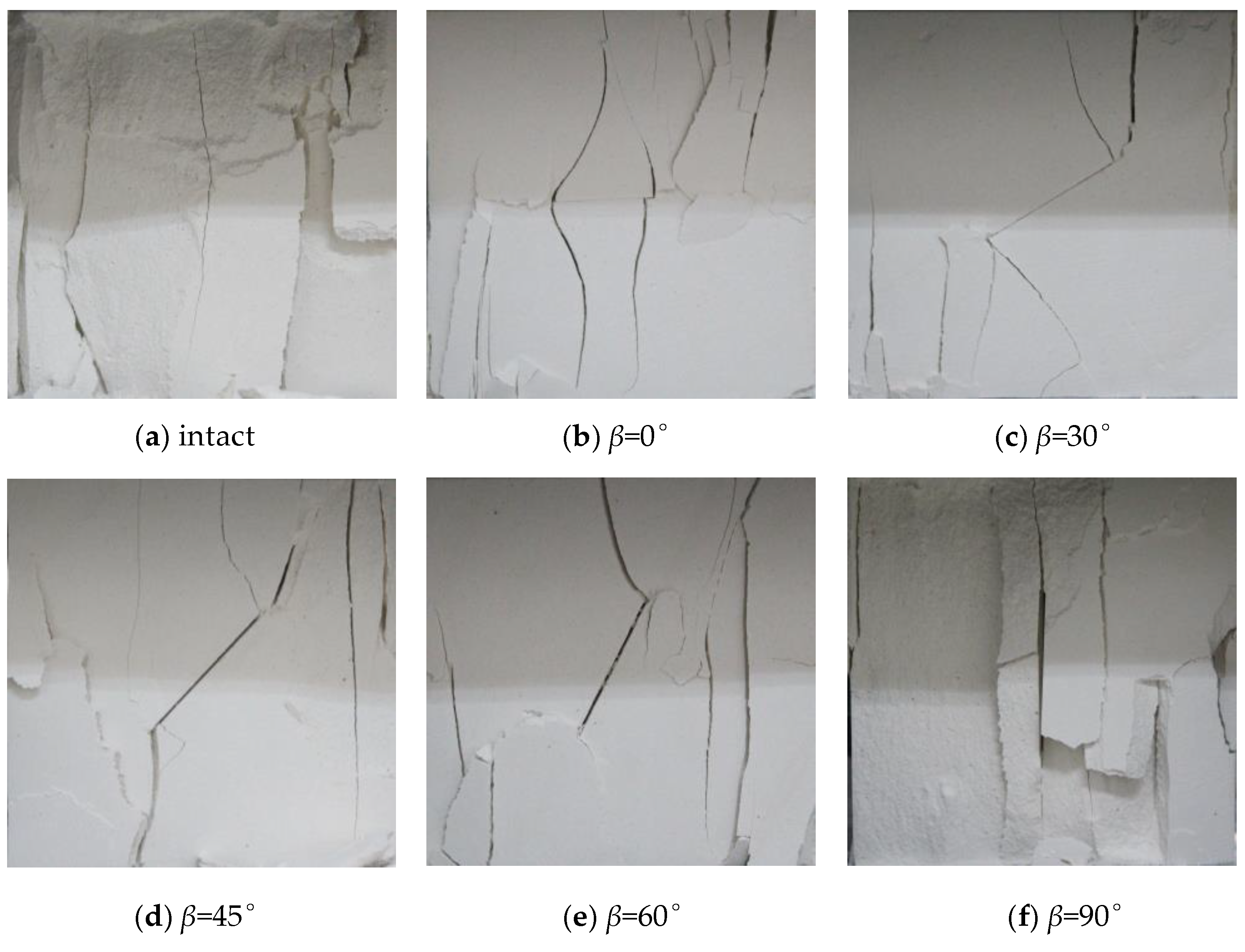
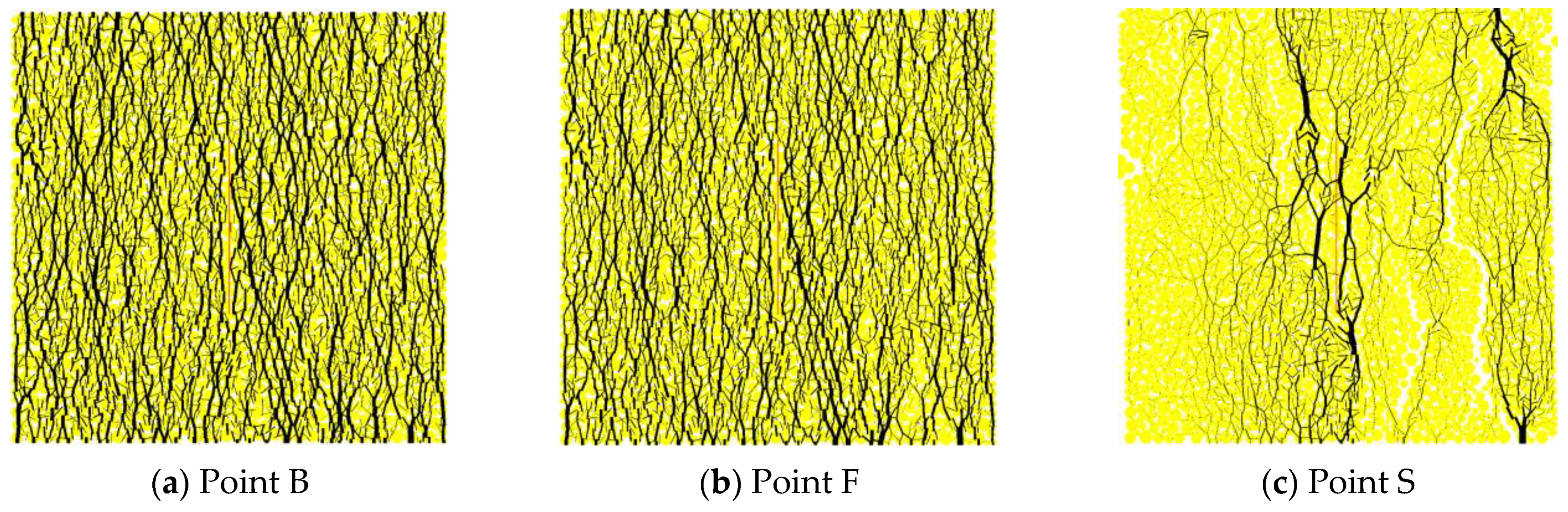
In the initial compaction stage (OA), the stress level is very low, and the internal micro-fractures and pores in the specimens are compressed, resulting in no or only a small amount of HPS. After the specimen is compacted, its deformation enters the elastic deformation stage (AB). The increasing stress in this stage is not enough to produce new cracks or to force the original micro-cracks to expand, so the HPS remains at a very small value. However, the AE energy of the specimen with β = 0° increases instantaneously in the form of a pulse in this stage, and the stress level does not increase or decrease significantly, that is, it is a non-corresponding point. Other researchers have also reported this phenomenon [36]. In the plastic deformation stage (BF), the variations in the stress and AE activity with time differ for the different specimens. For the specimens with low dip angles (β = 0°, 30°), the HPS increases rapidly in the form of a pulse at the beginning point or end point of this stage (points B and F, respectively). However, the HPS activity is stable at a low level and lasts for a long time, i.e., almost throughout the entire stage. For the specimens with β = 0°, the stress level fluctuates slightly when the HPS increases rapidly in the form of a pulse at point B (Figure 3b). For the specimens with medium inclination angles (β = 45°, 60°), the HPS exhibits a dense rapid increase in the form of a pulse throughout the entire stage. For the high joint angle specimens (β = 90°) and the intact specimens, the HPS increases rapidly in the form of a pulse at points B and F. However, in contrast to the specimens with low inclination angles, for the high joint angle specimens and intact specimens, the HPS distribution in the form of a pulse is denser, and the average value is larger near the peak strength (point F) of the stress–strain curve. The AE characteristics of the specimens with different inclination angles and the intact specimens may be related to the failure modes of the specimens. Figure 4 and Figure 5 show photos of the failure modes of the specimens at points F and S on the stress–strain curve, respectively.
- (1)
- For the specimens with low dip angles, for β = 0°, the failure mode was crushing; and in the plastic deformation stage, the propagation and coalescence of several thinner tensile cracks on the surface of the specimens occurred. These cracks were relatively small, the AE activity was dense throughout the entire stage, and the AE level was stable at a low level. For β = 30°, the failure mode was shear failure along the prefabricated joint plane. It had the smallest strength (7.34 MPa) compared with the jointed specimens with other angles, and the matrix damage was the lowest when the unstable failure occurred. Thus, the AE activity was weak and was only concentrated near the peak point.
- (2)
- For the specimens with medium inclination angles (β = 45° and 60°), which had a mixed type failure mode composed of shear failure and axial cleavage failure, the strength of the jointed specimens with inclination angles of 45° and 60° (8.31 MPa and 8.85 MPa, respectively) were between those of the specimens with inclination angles of 0° and 30°. In the plastic deformation stage, a large number of shear cracks formed in the specimens along the prefabricated joint plane. Furthermore, a long tensile crack formed along the loading axis (Figure 4d,e). Thus, the AE activity exhibited a dense rapid increase throughout the entire stage.
- (3)
- For the high joint angle specimens (β = 90°) and intact specimens, the failure mode was axial cleavage failure, which had a high strength compared with the jointed specimens with other angles. The matrix damage was very high when the instability destruction occurred. Thus, the AE activity was denser, and the average value was larger and was near the peak point.
In the post-peak failure stage (FS), after the destruction of the specimen, the decreases in the stress and HPS were significant. With the unsteady development of rock dilatancy, many micro-cracks were initiated and propagated further, resulting in a slightly higher HPS than before the failure. A large amount of energy was released, and audible sounds were produced during this stage.
All of the specimens had a large increment of AE energy near the peak point of stress (Figure 3); and at this time, the surface of the specimen contained obvious macroscopic cracks (the red area in Figure 4). For the intact specimens, the thinner tensile cracks on the surface of the specimen extended along the parallel loading axis and the HPS and the increment of the AE energy were larger, indicating that most of the cracks were generated inside of the specimen. For β = 0°, several wing cracks that extended obliquely toward the upper and lower surfaces of the specimen occurred at the joint tip. For β = 30°, the wing cracks perpendicular to the tip of the pre-existing joint rapidly expanded toward the upper and lower surfaces of the specimen, and the tensile crack that developed from the upper surface of the specimen penetrated the tip of the joint. For β = 45°, many cracks were generated inside the upper right part of the matrix and spread toward the surface of the specimen. Most of these cracks interlaced with each other, causing slabbing of the specimen’s surface. For β = 60°, wing cracks occurred at the lower left joint tip, and the wing crack at the upper right joint tip became wider. A small amount of powder appeared in the prefabricated joint, indicating that the specimen experienced shear slip along the prefabricated joint plane. In addition, tensile cracks were generated in the matrix parallel to the loading axis, and they almost crossed the upper and lower surfaces of the specimen. For β = 90°, the initiation, propagation, and coalescence of the microcracks inside of the specimen resulted in slabbing of the entire left-hand surface of the specimen and swelling of the matrix on the right side of the joint.
3.2. Strength and Deformation Parameters
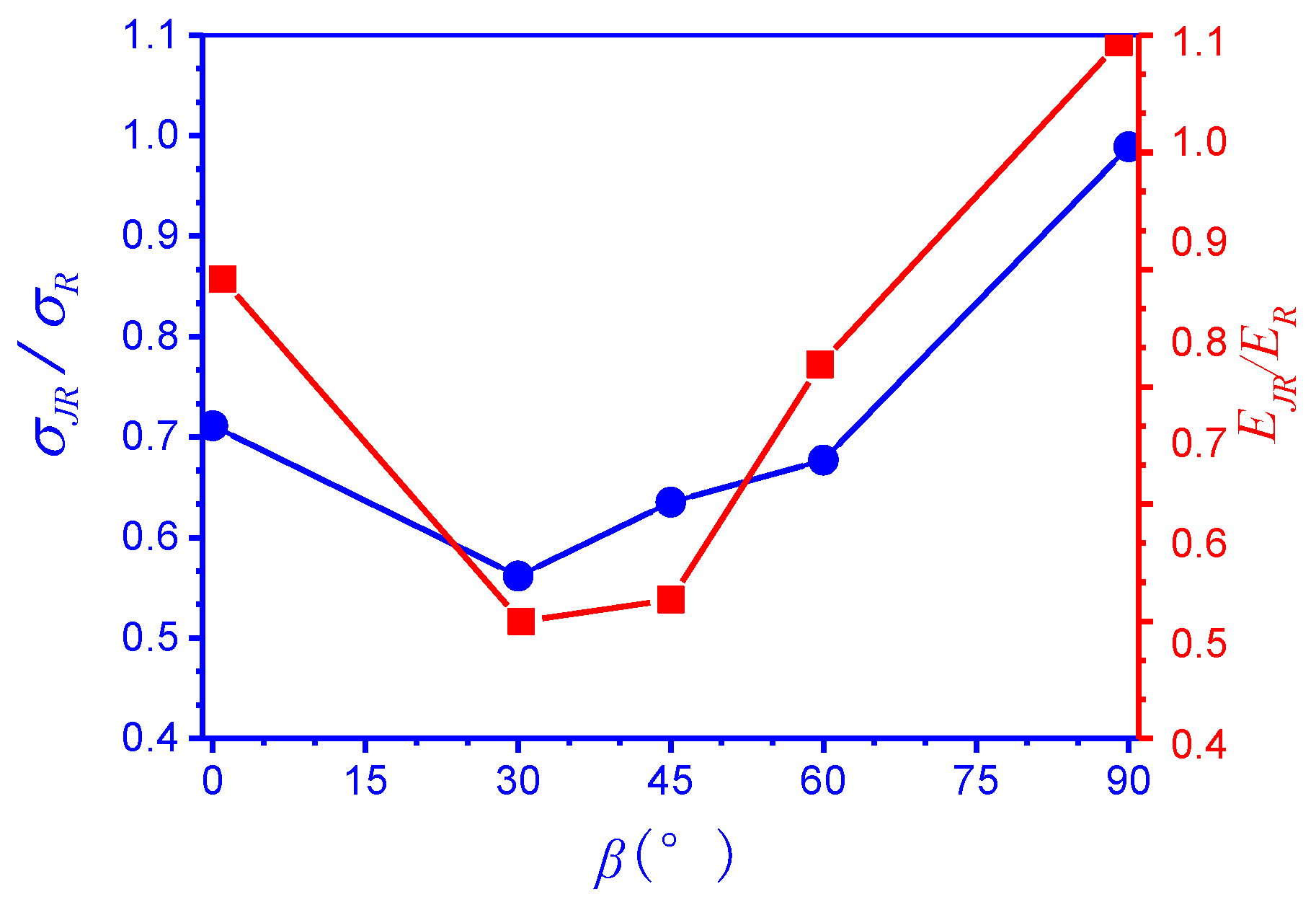
The unified peak strength () and the unified Young’s modulus () were introduced to reflect the trends in the peak strength and Young’s modulus with increasing joint inclination angle. Here, and are the peak strength and Young’s modulus of the jointed specimens, respectively; and and are those of the intact specimen, respectively. Figure 6 shows the variations in the and values with increasing joint dip angle (β). As can be seen, the variations in the unified peak strength () and the Young’s modulus () with β are V-shaped or U-shaped, with a minima at β = 30°.
Chen et al. [33] also found this relationship, but they found that the minima of the unified peak strength appeared at β = 45°. The reason for this difference may be related to the joint continuity factors [37]. Moreover, through uniaxial compression tests of specimens with closed joints, Han et al. [5] found that the variations in the peak strength and Young’s modulus with β were W-shaped, and thus, these variations may be affected by the open/closed state of the joint.
4. Numerical Models
4.1. Brief Introduction to the PFC2D Code and AE Simulation
Due to the variability in the AE signal parameters and the fact that the response of the pre-existing joint cannot be quantitatively analyzed in laboratory tests, PFC2D numerical modeling was used in this study. Cundall and Strack [38] introduced the idea of molecular dynamics based on the DEM and developed the particle discrete element theory. PFC2D is a software developed based on this theory. It can simulate the macroscopic strain-softening behaviors of rocks and the initiation, propagation, and coalescence of cracks during loading and unloading based on the microscopic responses between the particles and the bonds [39]. It is only necessary to define the micro-properties of the particles and bonds and the contact constitutive model in order to characterize the complex macroscopic mechanical properties, thereby avoiding the need to define the material macroscopic constitutive model.
PFC2D provides the linear parallel bond model and the smooth joint contact model. The linear parallel bond model can simulate a finite-sized piece of cementitious material between particles, which can transmit the contact forces and the moments between the particles. This characteristic is closer to the physical and mechanical properties of rock materials. The advantage of the smooth joint contact model is that the local contact direction between the particles can be ignored, that is, the particles can slide relatively easily along the joint direction [40]. In addition, the smooth joint contact model can also give an aperture a (a > 0 indicates that the joint is open), and it can monitor the joint opening or closing and the force acting on the joint plane during the loading process [32]. Therefore, in this study, the linear parallel bond model and the smooth joint contact model were used to simulate the matrix and the pre-existing joint in the rock, respectively. As is well known, microcracks usually generate AEs, which propagate through the rock and can be recorded to provide information about the cracks [16,41]. This phenomenon also occurs in the PFC. In the PFC2D models, the breakage of the contact bond (or microcrack) releases strain energy, and thus, it can generate AE activity. Consequently, the AE event can be simulated by counting the number of microcracks in the particle flow modeling [18].
4.2. Calibration of the Microparameters
A uniaxial numerical test was performed on an intact specimen to calibrate the microscopic properties of the particles and the parallel bonds in the rock matrix. The calibration of microscopic parameters was regarded as a “black-box problem”, and statistical methods were used to analyze the “input” and “output” information (i.e., microscopic parameters and macroscopic responses, respectively) of the particles and the parallel bonds, that is, the method of experimental design was used to determine the relationship between microscopic parameters and macroscopic responses, and an optimization method was used to determine the optimum set of microscopic parameters. This calibration method has been described by Yoon [42]. After the calibration test, the PFC2D model consisted of 2142 balls, and it was 60 mm in length and 60 mm in height. The microscopic parameters of the particles and the linear parallel bonds are presented in Table 3. The macroscopic properties of the intact specimen obtained from the numerical testing are very close to those obtained from the physical model testing (Table 4). Since a direct shear test of the joint has not been completed [43], the smooth joint parameters were calibrated using the trial-and-error method, which proved to be highly effective [32,33], and the results are shown in Table 5.
4.3. Analysis of the AE Test Results of the PFC2D Model
The AE signal was counted every 20 timesteps to study the failure processes of the specimens from a microscopic point of view, where the AE signal is the number of bond breakages (or the number of cracks) between the particles. The simulation results for the specimens with different inclination angles are shown in Figure 7.
On the stress–strain curve, there is no initial compression stage. The PFC2D model was constructed using an assembly of densely packed particles, and thus, microcrack closure did not occur in the dense and well-contacted assembly particles. Although the results of the numerical model and laboratory physical tests were not exactly the same, the PFC model of the brittle material has been shown to satisfactorily reproduce many of the mechanical behavior characteristics of this material under different stress conditions [16].
In Figure 7, the stress–strain curve can be divided into three stages: the elastic deformation stage (AB), the plastic deformation stage (BF), and the post-peak failure stage (FS). The AE phenomenon observed in each stage is basically the same as that observed in the physical experiments. That is, in stage AB, the number of cracks in the early part of this stage was zero, and then, it remained at a low value. In stage BF, the number of cracks began to increase rapidly and entered an unstable state, and then, it reached an instantaneous maximum. In stage FS, the number of cracks decreased significantly, but it was slightly higher than that before failure.
Moreover, as is shown in Figure 7, the evolution curves of the AE characteristics of the specimens with β = 0° and 30° are approximately single peak type, and the peak point corresponds to point F on the stress–strain curve. The evolution curves of the AE characteristics of the specimens with β = 45°, 60°, and 90° are the double peak type, and the first peak point and the second peak point correspond to point F and the FS stage on the stress–strain curve, respectively. That is, as the joint inclination angle increases, the AE characteristic evolution curve gradually transforms from a single peak type curve to a double peak type curve. For the specimens with medium and high inclination angles, the generation of the second peak point on the evolution curves of the AE characteristics is closely related to the response of the pre-existing joint, which is fully analyzed in Section 4.4.
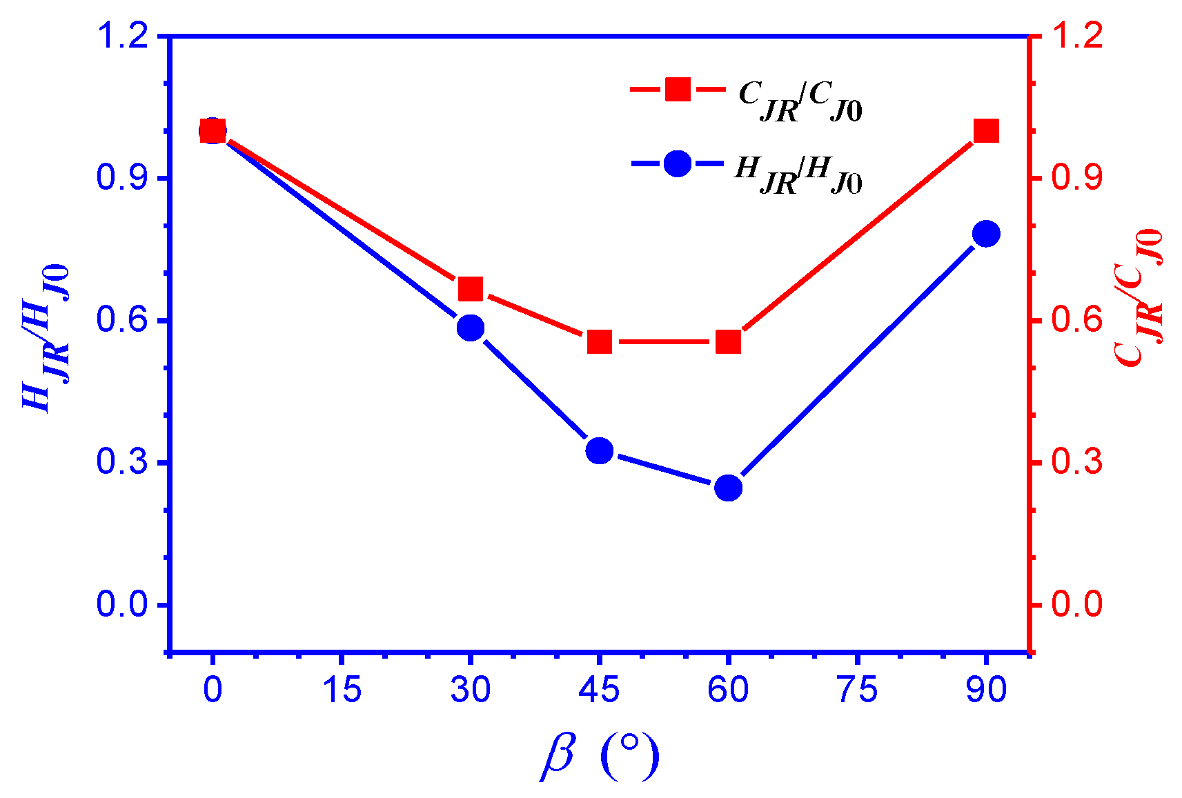
The unified HPS () and the unified crack number () at the peak strength were introduced to reflect the variation in the AE activity at the peak strength point with increasing joint inclination angle. Here, and are the HPS and the number of cracks at the peak strength of the jointed specimens, respectively; and and are those of the specimen with β = 0°, respectively. Figure 8 shows the variations in and with increasing joint dip angle (β). As can be seen, the variations in the unified HPS () and the unified crack number () with β are V-shaped or U-shaped, with a minima at β = 45°. The AE activity results obtained from the laboratory physical tests and the numerical simulations are consistent, which once again verifies the validity of the PFC2D model.
4.4. Response of the Pre-Existing Joint
From the laboratory physical tests, it was found that the AE activity may be related to the failure mode of the jointed specimens with different inclination angles, and the failure mode is closely related to the response of the pre-existing joint. Therefore, the mechanical response of the joint was quantitatively analyzed to study the damage mechanism of the jointed specimens and the relationship between the pre-existing joint and the AE activity.
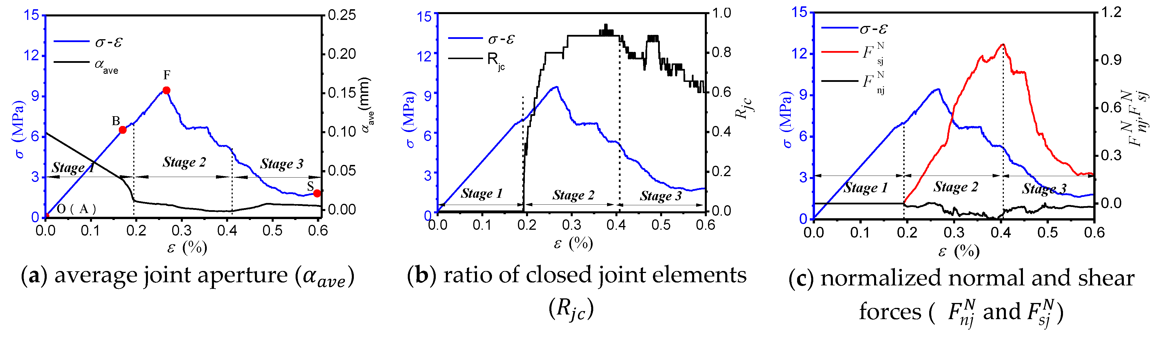
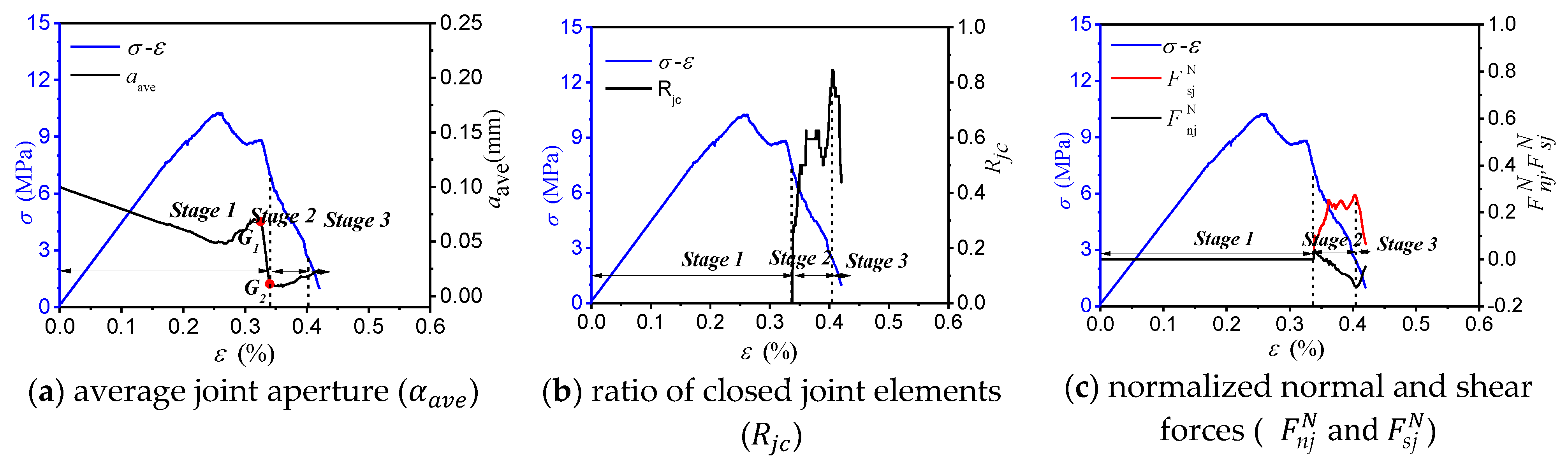
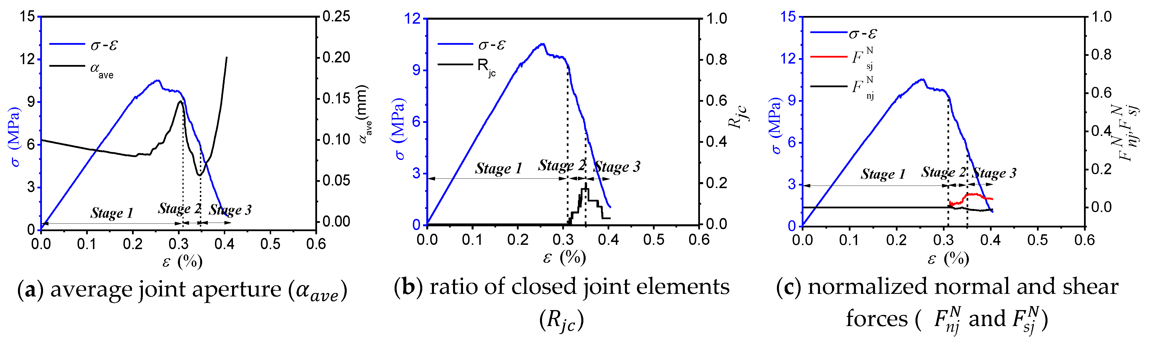
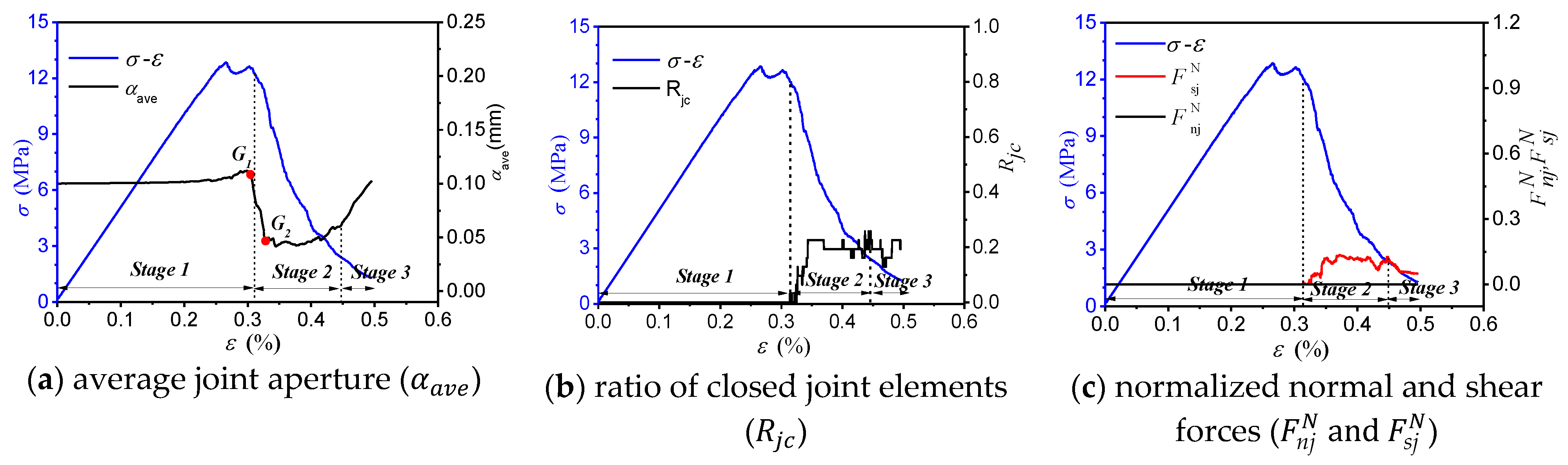
Cheng et al. [32] and Chen et al. [33] defined the following three parameters for the joint elements in a joint system to further investigate the role of joints with different inclination angles throughout the entire failure process: the average joint aperture () and the sum of the current value of the joint element apertures () divided by the total number of joint elements (N).
where an increase or decrease in represents the opening or closing of the joint element, respectively. Therefore, is used to estimate whether the overall trend of the joint system is opening or closing.
The ratio of the closed joint elements () is defined as the number of closed joint elements () divided by the total number of joint elements (N):
where indicates that the joint element is closed. is a normalized index used to evaluate the closure status of the joint system.
The normalized normal and shear forces acting on the joint elements ( and , respectively) are defined as the total normal and shear contact forces of the joint elements in a specimen ( and , respectively) divided by the maximum value of the total normal contact forces of the joint elements in all of the specimens (, that is, that of the specimen with β = 0°).
Based on the above three parameters of the pre-existing joint and the evolution of the force chain distribution at the key points on the stress–strain curve, the mechanical response of the pre-existing joint can be studied (Figure 9, Figure 10, Figure 11, Figure 12, Figure 13, Figure 14, Figure 15, Figure 16, Figure 17 and Figure 18). The response of the pre-existing joint mainly involves three stages: (I) the closing of the joint; (II) the strength mobilization of the joint; and (III) the reopening of the joint.
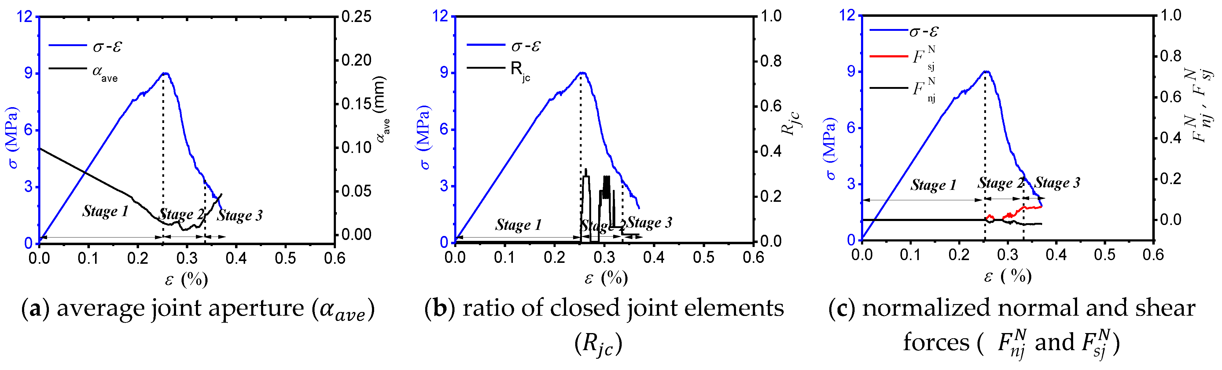
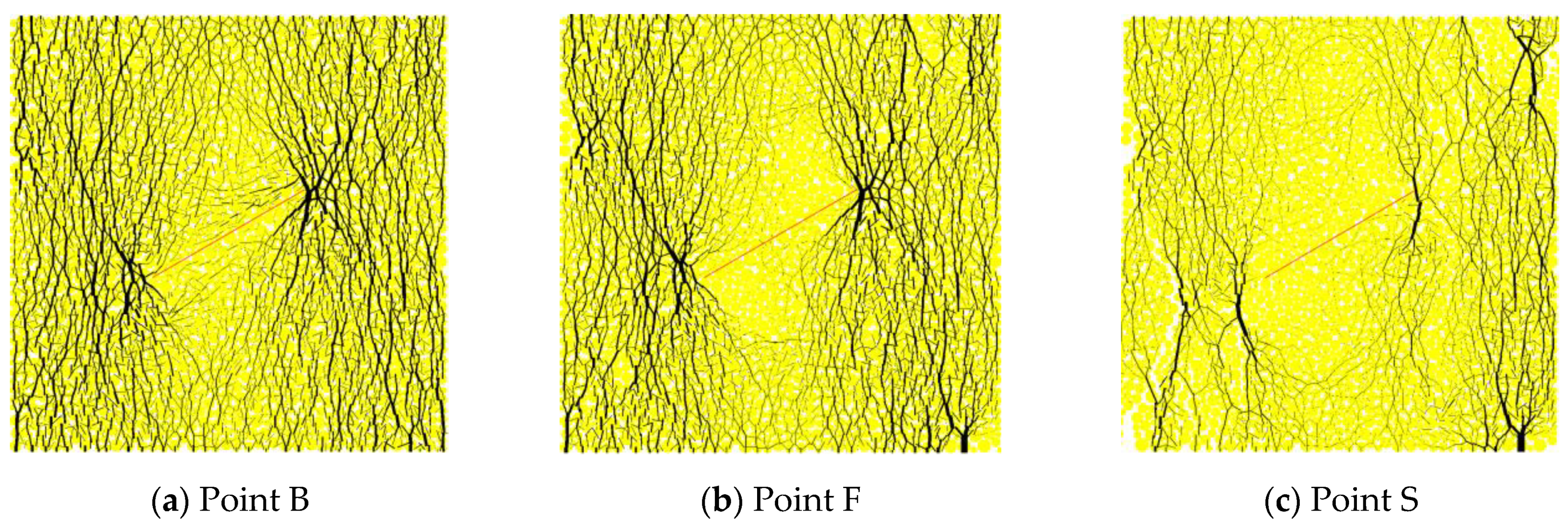
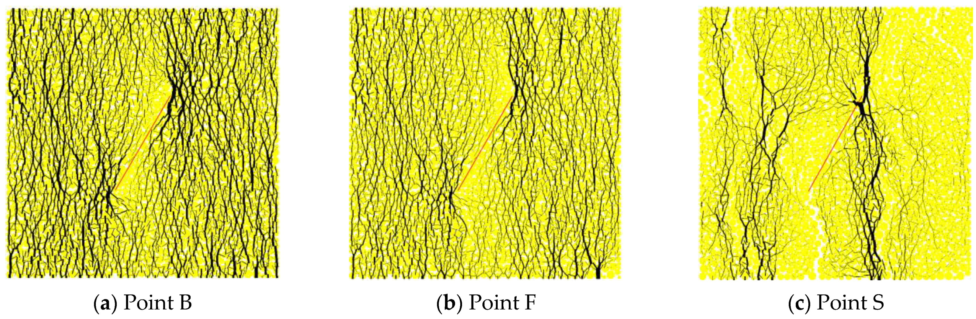
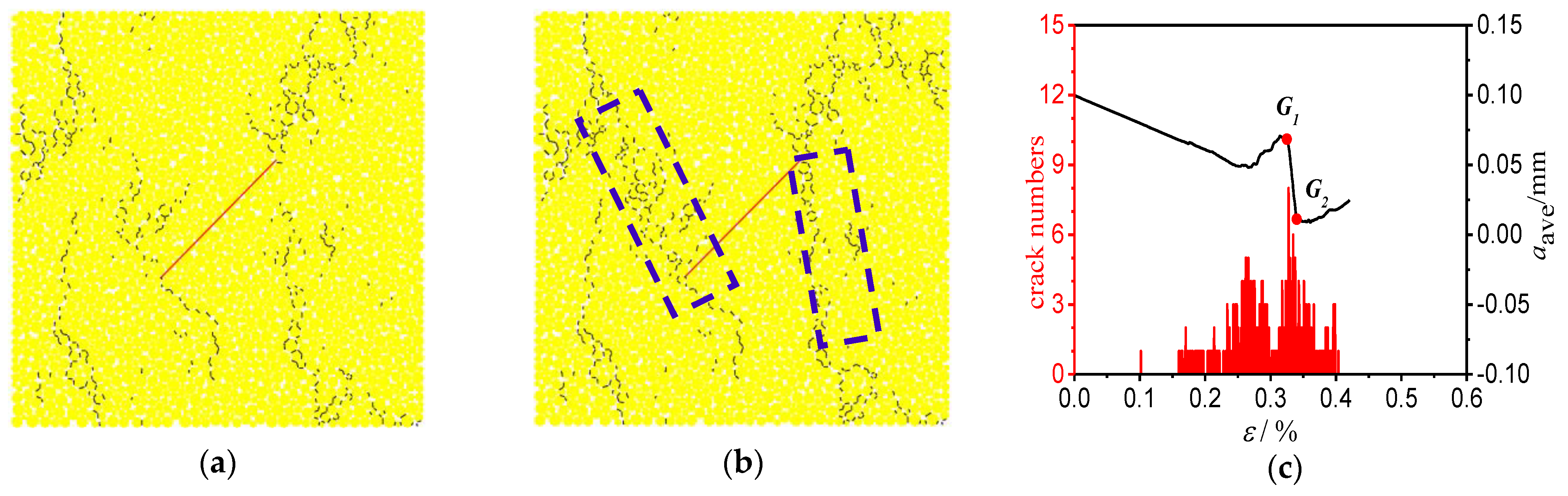
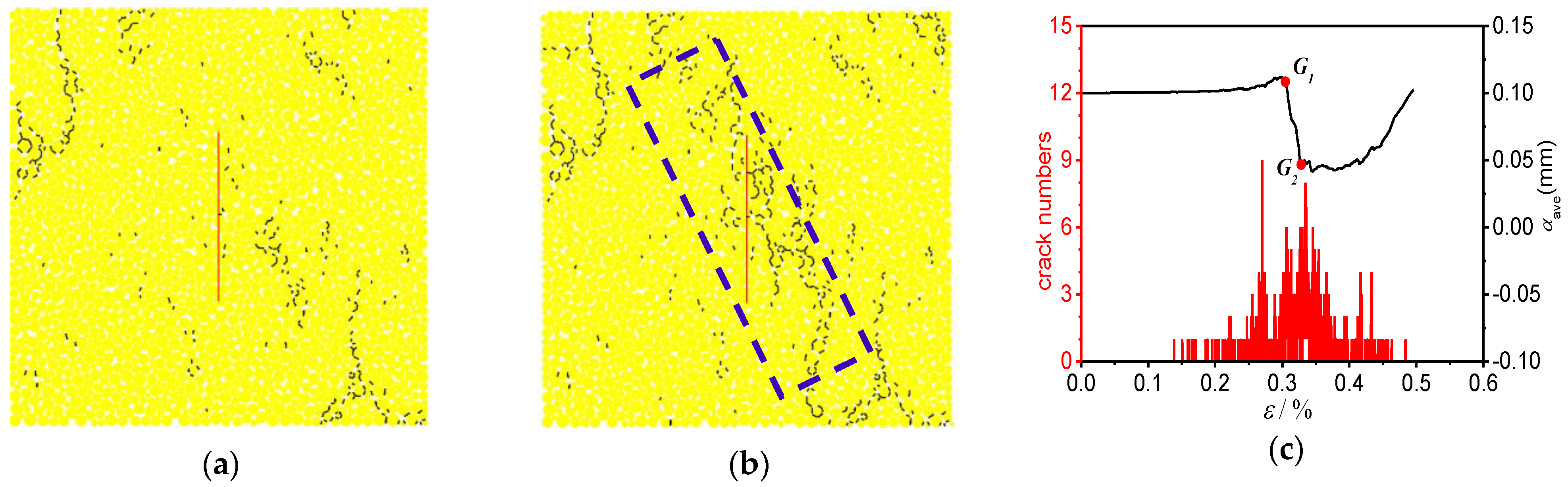
Stage I: For the specimens with small dip angles (β = 0° and 30°), the average joint aperture () decreases rapidly. Based on the force chain distribution at point B (Figure 10a and Figure 12a), the stress concentration at the joint tips and the stress arches in the matrix can be found. For β = 0°, this stage almost coincided with the elastic deformation stage of the stress–strain curve; however, for β = 30°, this stage coincided with the pre-peak stage of the stress–strain curve. For the specimens with medium inclination angles (β = 45°and 60°), in the early part of this stage, which coincided with the pre-peak stage of the stress–strain curve, the decrease in speed was obviously smaller than that of the specimens with small inclination angles. Based on the force chain distribution at points B and F (Figure 14a,b and Figure 16a,b), the stress concentration appears at the joint tips, and the stress in the matrix gradually transitions from a uniform distribution to localization. In the later part of this stage, which coincided with the yield stage on the post-peak portion of the stress–strain curve, increased rapidly, which may be caused by the dilation. For β = 45°, increased rapidly and then decreased instantaneously. Figure 19a–c show the breakage distribution of the contact bonds in the matrix of the specimen at and , and the variation trends of and the number of crack elements over the axial strain. It was found that at and , the AE activity was very strong, and the connection between the joint tips and macrocracks formed by the initiation, propagation, and coalescence of the microcracks lead to joint sliding, and thus, decreased sharply. For the high joint angle specimens, did not significantly decrease in this stage, and the stress distribution in the matrix was uniform (Figure 18a,b). For all of the jointed specimens, , , and remained at zero, indicating that the joint elements were closing, but none of them had fully closed yet in this stage, and they could not transfer any of the normal or shear forces.
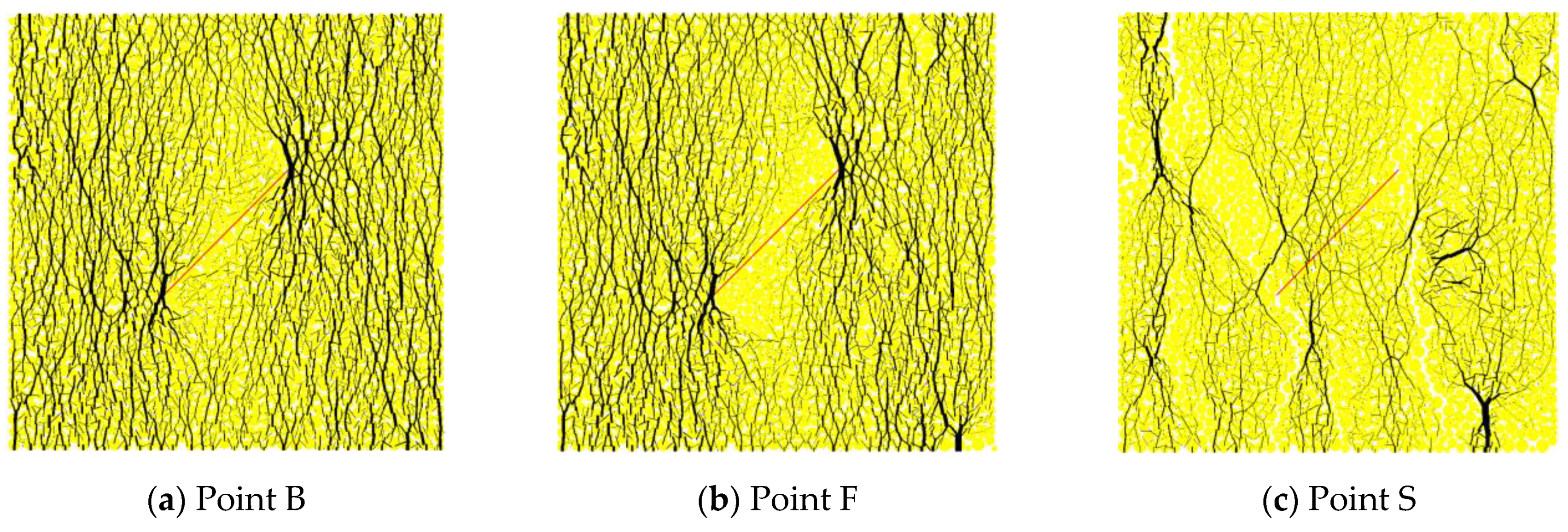
Stage II: For all of the jointed specimens, reached its minimum in this stage. For the jointed specimens with β = 60° and 90°, instantaneously decreased. The reason this phenomenon occurred for the specimens with β = 60° is the same as that for the specimens with β = 45° in stage I. For β = 90°, Figure 20a–c shows the breakage distribution of the contact bonds in the matrix of the specimen at and , the variation in , and the number of crack elements over the axial strain. It was found that the AE activity was very strong, and the macrocracks formed through the initiation, propagation, and coalescence of microcracks across the pre-existing joint plane along the vertical loading direction. Therefore, the joint plane and the local matrix around it were destroyed. Due to the dilation, the block of matrix near the damaged joint plane moved, which caused to instantaneously decrease. For all of the jointed specimens, and increased rapidly and reached their maximum values in this stage, indicating that the pre-existing joint had been closed and could transfer the normal force. Among the specimens, the and values were the largest for the specimen with β = 0°, indicating that the strength mobilization of the pre-existing joint in the specimen with β = 0° was the most adequate. It should be noted that although the of the specimen with β = 45° was larger in this stage, was smaller, indicating that although many of the joint elements were closed in the specimen, the strength of these closed joint elements was very small, so the strength mobilization of the pre-existing joint in the specimen with β = 45° was inadequate.
Stage III: For all of the jointed specimens, increased, and and decreased. For the specimen with β = 0°, the increase of was very small, and remained at a high level throughout the entire stage, indicating that the closed joint system maintained a high degree in this stage (Figure 10c). For the other jointed specimens, increased rapidly, and and decreased to zero or remained at very small values, indicating that the strength mobilization of the pre-existing joint was almost completely degraded (Figure 12c, Figure 16c and Figure 18c).
In addition, by observing the variation trends of and over the axial strain for all of the specimens, it was found that the strength mobilization of the pre-existing joint in the specimen with β = 0° started at the beginning of the plastic deformation stage. For β = 30°, it started at about the peak strength. For β = 45°, 60°, and 90°, it started in the post-peak stage. That is, as the joint inclination angle of the specimens increased, the strength mobilization of the pre-existing joint gradually shifted from the pre-peak stage of the stress–strain curve to the post-peak stage.
5. Conclusions
In this study, the correlation between the AE activity and the failure modes of pre-cracked specimens was investigated through laboratory AE tests. PFC modeling was carried out to reproduce the phenomena observed in the physical experiments. For the jointed specimens and intact specimen, the characteristics of the AE activity, the response of the pre-existing joints, and the relationship between them were analyzed.
For the specimens with a single pre-existing flaw, the inclination angles β = 0°, 30°, 45°, 60°, and 90° were used. The HPS and energy were used to evaluate the AE activities in the laboratory tests. The smooth-joint contact model and the linear parallel bond model were selected for the pre-existing joints and the matrix, respectively. The microparameters of the particles and contacts in the PFC2D model were calibrated using the results of the physical experiments. Then, the AE activity was simulated by the bond breakage (or microcracks). The mechanical response of the pre-existing joint was monitored using three parameters for the pre-existing joint, i.e., the average joint aperture (), the ratio of the closed joint elements (), and the normalized normal and shear forces acting on the joint elements ( and , respectively). The following conclusions were drawn from the results.
- The AE characteristics have a good correlation with the failure mode of the specimens with different inclination angles. In the plastic deformation stage of the stress–strain curve, for the specimens with small inclination angles (β = 0°, 30°), the AE activity was stable at a low level and lasted for a long time, and the failure modes were crushing (β = 0°) and shear failure (β = 30°). For the specimens with medium inclination angles (β = 45°, 60°), the AE exhibited a dense rapid increase in the form of a pulse throughout the entire stage, and it had a mixed type failure mode consisting of shear failure and axial cleavage failure. For the high joint angle specimens (β = 90°) and intact specimens, the AE distribution was a pulse, which was denser and had a larger average value near the peak point (point F), and the failure mode was axial cleavage failure.
- The variations in the peak strength and the Young’s modulus with β are V-shaped or U-shaped, with a minima and maxima at β = 30° and 90°, respectively.
- As the joint inclination angle increased, the AE characteristic evolution curve gradually transformed from a single peak type curve to a double peak type curve. For the specimens with medium and high inclination angles, the generation of the second peak point on the evolution curve of the AE characteristics was closely related to the response of the pre-existing joint.
- In the post-peak failure stage (FS), for the specimens with medium and high inclination angles (β = 45°, 60° and 90°), the stronger AE activity corresponded to an instantaneous decrease in the average joint aperture (), which was related to the failure mode of the specimens.
- The response of the pre-existing joint in the numerical model can be divided into three stages based on the varied mobilization of the joint strength: (I) the closing of the pre-existing joint; (II) the strength mobilization of the pre-existing joint; and (III) the reopening of the pre-existing joint. As the joint inclination angle increased, the strength mobilization stage of the joint system gradually shifted from the pre-peak stage of the stress-strain curve to the post-peak stage.
Author Contributions
Conceptualization, Z.F. and X.C.; Data curation, Z.F. and T.X.; Investigation, Z.F.; Writing – original draft, Z.F. and Y.F.; Software, S.Q. All authors have read and agreed to the published version of the manuscript.
Funding
This research was financially supported by the National Natural Science Foundation of China (No. 41941018 and No. 11572344) and the National Key Research and Development Program of China (No. 2016YFC0600901).
Acknowledgments
We thank C. Cheng from the School of Engineering and Technology, China University of Geosciences (Beijing) for his help with the PFC modeling.
Conflicts of Interest
On behalf of all of the authors, the corresponding author declares that there is no conflict of interest.
References
- Cai, M.; Kaiser, P.K.; Martin, C.D. Quantification of rock mass damage in underground excavations from microseismic event monitoring. Int. J. Rock Mech. Min. Sci. 2001, 38, 1135–1145. [Google Scholar] [CrossRef]
- Li, S.L.; Tang, H.Y. Acoustic emission characteristics in failure process of rock under different uniaxial compressive loads. Yantu Gongcheng Xuebao Chin. J. Geotech. Eng. 2010, 32, 147–152. [Google Scholar]
- Blake, W. Microseismic Applications for Mining–A Practical Guide; Bureau of Mines: Washington, DC, USA, 1982.
- Kong, B.; Wang, E.; Li, Z.; Wang, X.; Niu, Y.; Kong, X. Acoustic emission signals frequency-amplitude characteristics of sandstone after thermal treated under uniaxial compression. J. Appl. Geophys. 2017, 136, 190–197. [Google Scholar] [CrossRef]
- Han, G.; Jing, H.; Jiang, Y.; Liu, R.; Su, H.; Wu, J. The effect of joint dip angle on the mechanical behavior of infilled jointed rock masses under uniaxial and biaxial compressions. Processes 2018, 6, 49. [Google Scholar] [CrossRef] [Green Version]
- Meng, Q.; Zhang, M.; Han, L.; Pu, H.; Nie, T. Effects of Acoustic Emission and Energy Evolution of Rock Specimens Under the Uniaxial Cyclic Loading and Unloading Compression. Rock Mech. Rock Eng. 2016, 49, 3873–3886. [Google Scholar] [CrossRef]
- Wang, J.; Xie, L.; Xie, H.; Ren, L.; He, B.; Li, C.; Yang, Z.; Gao, C. Effect of layer orientation on acoustic emission characteristics of anisotropic shale in Brazilian tests. J. Nat. Gas. Sci. Eng. 2016, 36, 1120–1129. [Google Scholar] [CrossRef]
- Ishida, T.; Kanagawa, T.; Kanaori, Y. Source distribution of acoustic emissions during an in-situ direct shear test: Implications for an analog model of seismogenic faulting in an inhomogeneous rock mass. Eng. Geol. 2010, 110, 66–76. [Google Scholar] [CrossRef] [Green Version]
- Wang, H.; Liu, D.; Cui, Z.; Cheng, C.; Jian, Z. Investigation of the fracture modes of red sandstone using XFEM and acoustic emissions. Theor. Appl. Fract. Mech. 2016, 85, 283–293. [Google Scholar] [CrossRef]
- Katsuyama, K. Application of AE techniques; Metallurgy Industry Press: Beijing, China, 1996. [Google Scholar]
- Holcomb, D.J.; Costin, L.S. Detecting damage surfaces in brittle materials using acoustic emissions. J. Appl. Mech. Trans. ASME 1986, 53, 536–545. [Google Scholar] [CrossRef]
- Pestman, B.J.; Van Munster, J.G. An acoustic emission study of damage development and stress-memory effects in sandstone. Int. J. Rock Mech. Min. Sci. Geomech. 1996, 33, 585–593. [Google Scholar] [CrossRef]
- Liu, T.; Lin, B.; Yang, W. Mechanical behavior and failure mechanism of pre-cracked specimen under uniaxial compression. Tectonophysics 2017, 712–713, 330–343. [Google Scholar] [CrossRef]
- Jiang, Y.; Luan, H.; Wang, D.; Wang, C.; Han, W. Failure Mechanism and Acoustic Emission Characteristics of Rock Specimen with Edge Crack Under Uniaxial Compression. Geotech. Geol. Eng. 2019, 37, 2135–2145. [Google Scholar] [CrossRef]
- Li, D.; Wang, E.; Kong, X.; Ali, M.; Wang, D. Mechanical behaviors and acoustic emission fractal characteristics of coal specimens with a pre-existing flaw of various inclinations under uniaxial compression. Int. J. Rock Mech. Min. Sci. 2019, 116, 38–51. [Google Scholar] [CrossRef]
- Hazzard, J.F.; Young, R.P. Simulating acoustic emissions in bonded-particle models of rock. Int. J. Rock Mech. Min. Sci. 2000, 37, 867–872. [Google Scholar] [CrossRef]
- Hazzard, J.F.; Young, R.P. Dynamic modelling of induced seismicity. Int. J. Rock Mech. Min. Sci. 2004, 41, 1365–1376. [Google Scholar] [CrossRef]
- Su, H.; Dang, C.H.; Li, Y.J. Study of numerical simulation of acoustic emission in rock of inhomogeneity. Yantu Lixue Rock Soil Mech. 2011, 32, 1886–1890. [Google Scholar] [CrossRef]
- Wang, P.; Yang, T.; Xu, T.; Cai, M.; Li, C. Numerical analysis on scale effect of elasticity, strength and failure patterns of jointed rock masses. Geosci. J. 2016, 20, 539–549. [Google Scholar] [CrossRef]
- Cai, M.; Kaiser, P.K.; Morioka, H.; Minami, M.; Maejima, T.; Tasaka, Y.; Kurose, H. FLAC/PFC coupled numerical simulation of AE in large-scale underground excavations. Int. J. Rock Mech. Min. Sci. 2007, 44, 550–564. [Google Scholar] [CrossRef]
- Shang, J.; Hencher, S.R.; West, L.J. Tensile Strength of Geological Discontinuities Including Incipient Bedding, Rock Joints and Mineral Veins. Rock Mech. Rock Eng. 2016, 49, 4213–4225. [Google Scholar] [CrossRef] [Green Version]
- Wasantha, P.L.P.; Ranjith, P.G.; Xu, T.; Zhao, J.; Yan, Y.L. A new parameter to describe the persistency of non-persistent joints. Eng. Geol. 2014. [Google Scholar] [CrossRef]
- Wong, R.H.C.; Chau, K.T.; Tang, C.A.; Lin, P. Analysis of crack coalescence in rock-like materials containing three flaws—Part I: Experimental approach. Int. J. Rock Mech. Min. Sci. 2001, 38, 909–924. [Google Scholar] [CrossRef]
- Zhang, H.Q.; Zhao, Z.Y.; Tang, C.A.; Song, L. Numerical study of shear behavior of intermittent rock joints with different geometrical parameters. Int. J. Rock Mech. Min. Sci. 2006. [Google Scholar] [CrossRef]
- Gehle, C.; Kutter, H.K. Breakage and shear behaviour of intermittent rock joints. Int. J. Rock Mech. Min. Sci. 2003. [Google Scholar] [CrossRef]
- Halakatevakis, N.; Sofianos, A.I. Strength of a blocky rock mass based on an extended plane of weakness theory. Int. J. Rock Mech. Min. Sci. 2010. [Google Scholar] [CrossRef]
- Jiang, Y.; Li, B.; Yamashita, Y. Simulation of cracking near a large underground cavern in a discontinuous rock mass using the expanded distinct element method. Int. J. Rock Mech. Min. Sci. 2009. [Google Scholar] [CrossRef] [Green Version]
- Kulatilake, P.H.S.W.; Ucpirti, H.; Wang, S.; Radberg, G.; Stephansson, O. Use of the distinct element method to perform stress analysis in rock with non-persistent joints and to study the effect of joint geometry parameters on the strength and deformability of rock masses. Rock Mech. Rock Eng. 1992. [Google Scholar] [CrossRef]
- Ghazvinian, A.; Sarfarazi, V.; Schubert, W.; Blumel, M. A study of the failure mechanism of planar non-persistent open joints using PFC2D. Rock Mech. Rock Eng. 2012. [Google Scholar] [CrossRef]
- Fan, X.; Kulatilake, P.H.S.W.; Chen, X. Mechanical behavior of rock-like jointed blocks with multi-non-persistent joints under uniaxial loading: A particle mechanics approach. Eng. Geol. 2015. [Google Scholar] [CrossRef]
- Sagong, M.; Park, D.; Yoo, J.; Lee, J.S. Experimental and numerical analyses of an opening in a jointed rock mass under biaxial compression. Int. J. Rock Mech. Min. Sci. 2011, 48, 1055–1067. [Google Scholar] [CrossRef]
- Cheng, C.; Chen, X.; Zhang, S. Multi-peak deformation behavior of jointed rock mass under uniaxial compression: Insight from particle flow modeling. Eng. Geol. 2016, 213, 25–45. [Google Scholar] [CrossRef]
- Chen, X.; Zhang, S.; Cheng, C. Numerical study on effect of joint strength mobilization on behavior of rock masses with large nonpersistent joints under uniaxial compression. Int. J. Geomech. 2018, 18, 1–21. [Google Scholar] [CrossRef]
- Shang, J. Rupture of Veined Granite in Polyaxial Compression: Insights From Three-Dimensional Discrete Element Method Modeling. J. Geophys. Res. Solid Earth 2020, 125, e2019JB019052. [Google Scholar] [CrossRef]
- Wang, S.; Liu, Y.; Chen, X.; Yang, Q. Failure analysis of pre-cracked specimen based on acoustic emission technique. Shuili Fadian Xuebao J. Hydroelectr. Eng. 2019, 38, 110–120. [Google Scholar] [CrossRef]
- Song, Y.; Xing, T.; Zhao, T.; Zhao, Z.; Gao, P. Acoustic emission characteristics of deformation field development of rock under uniaxial loading. Yanshilixue Yu Gongcheng Xuebao Chin. J. Rock Mech. Eng. 2017, 36, 534–542. [Google Scholar] [CrossRef]
- Chen, X.; Liao, Z.H.; Peng, X. Cracking process of rock mass models under uniaxial compression. J. Cent. South. Univ. 2013, 20, 1661–1678. [Google Scholar] [CrossRef]
- Cundall, P.A.; Strack, O.D.L. A discrete numerical model for granular assemblies. Geotechnique 1980, 30, 331–336. [Google Scholar] [CrossRef] [Green Version]
- Potyondy, D.O.; Cundall, P.A. A bonded-particle model for rock. Int. J. Rock Mech. Min. Sci. 2004, 41, 1329–1364. [Google Scholar] [CrossRef]
- Mas Ivars, D.; Pierce, M.E.; Darcel, C.; Reyes-Montes, J.; Potyondy, D.O.; Paul Young, R.; Cundall, P.A. The synthetic rock mass approach for jointed rock mass modelling. Int. J. Rock Mech. Min. Sci. 2011, 48, 219–244. [Google Scholar] [CrossRef]
- Hazzard, J.F.; Young, R.P.; Maxwell, S.C. Micromechanical modeling of cracking and failure in brittle rocks. J. Geophys. Res. Solid Earth 2000, 105, 16683–16697. [Google Scholar] [CrossRef]
- Yoon, J. Application of experimental design and optimization to PFC model calibration in uniaxial compression simulation. Int. J. Rock Mech. Min. Sci. 2007, 44, 871–889. [Google Scholar] [CrossRef]
- Shang, J.; Zhao, Z.; Hu, J.; Handley, K. 3D Particle-Based DEM Investigation into the Shear Behaviour of Incipient Rock Joints with Various Geometries of Rock Bridges. Rock Mech. Rock Eng. 2018, 51, 3563–3584. [Google Scholar] [CrossRef]
Figure 1.
(a) Sketches of specimen’s geometry and joint geometry; (b) photograph of a sample (β = 60°).
Figure 1.
(a) Sketches of specimen’s geometry and joint geometry; (b) photograph of a sample (β = 60°).

Figure 2.
Arrangement of the AE sensors.

Figure 3.
The variations in the stress, hits per second (HPS), and energy accumulation over time for samples with different inclination angles.
Figure 3.
The variations in the stress, hits per second (HPS), and energy accumulation over time for samples with different inclination angles.


Figure 4.
Photographs of specimens at selected key point F in the stress–strain curve.

Figure 5.
Photographs of specimens at selected key point S in the stress–strain curve.

Figure 6.
Variations in and with increasing joint inclination angle (β).

Figure 7.
Stress–strain and HPS–strain curves for samples with different crack angles.


Figure 8.
Variations in and with increasing inclination angle (β).

Figure 9.
Evolution of the parameters of the joint system with increasing axial strain ( = 0°).

Figure 10.
Evolution of force chain distribution with axial strain increases ( = 0°)

Figure 11.
Evolution of the parameters of the joint system with increasing axial strain ( = 30°).

Figure 12.
Evolution of force chain distribution with axial strain increases ( = 30°).

Figure 13.
Evolution of the parameters of the joint system with increasing axial strain ( = 45°)

Figure 14.
Evolution of force chain distribution with axial strain increases ( = 45°).

Figure 15.
Evolution of the parameters of the joint system with increasing axial strain ( = 60°).

Figure 16.
Evolution of force chain distribution with axial strain increases ( = 60°).

Figure 17.
Evolution of the parameters of the joint system with increasing axial strain ( = 90°).

Figure 18.
Evolution of force chain distribution with axial strain increases ( = 90°).

Figure 19.
Breakage distribution of contact bonds in the matrix of the specimen with β = 45° at (a) Point and (b) Point , and (c) the variation trends of and the number of crack elements over axial strain.
Figure 19.
Breakage distribution of contact bonds in the matrix of the specimen with β = 45° at (a) Point and (b) Point , and (c) the variation trends of and the number of crack elements over axial strain.

Figure 20.
Breakage distribution of contact bonds in the matrix of the specimen with β = 90° at (a) point and (b) point , and (c) the variation trends of and the number of crack elements over axial strain.
Figure 20.
Breakage distribution of contact bonds in the matrix of the specimen with β = 90° at (a) point and (b) point , and (c) the variation trends of and the number of crack elements over axial strain.


Table 1.
Physical and mechanical properties of the modeled material.
| Unit Weight γ (kN/m3) | UCS (MPa) | Young’s Modulus E (GPa) | Poisson’s Ratio v | Cohesion c (MPa) | Internal Friction Angle φ (°) |
|---|---|---|---|---|---|
| 11.69 | 12.54 | 5.6 | 0.23 | 3.0 | 34 |
Table 2.
The definitions of the characteristic points on the stress–strain curve.
| Characteristic Points | Definition |
|---|---|
| O | Start point of test |
| A | Start point of elastic deformation |
| B | Start point of plastic deformation |
| F | Peak strength point |
| S | End point of test |
Table 3.
Microscopic properties of the particles and bonds.
| Ball Parameters | Value | Parallel Bond Parameters | Value |
|---|---|---|---|
| Ball density [ (kg/m3)] | 1169 | Bond modulus [ (GPa)] | 4.17 |
| Minimum ball radius [ (mm)] | 0.6 | Normal bond strength [ (MPa)] | 9.2 |
| Ball radius ratio () | 1.66 | S.D. normal bond strength [ (MPa)] | 3.78 |
| Contact modulus [ (GPa)] | 4.17 | Cohesion [ (MPa)] | 20 |
| Friction coefficient (μ) | 0.5 | S.D. cohesion [ (MPa)] | 5.0 |
| Normal to shearing stiffness ratio () | 2.5 | Friction angle (°) | 30 |
| Normal to shearing bond stiffness ratio () | 2.5 |
Table 4.
Comparisons of the experimentally and numerically calibrated macroscopic properties.
| Macroscopic Properties | Experimental | Numerical |
|---|---|---|
| Uniaxial compressive strength [UCS (MPa)] | 13.08 | 13.20 |
| Young’s modulus [E (GPa)] | 5.03 | 4.38 |
Table 5.
Microscopic properties of the smooth-joint contact of a pre-existing joint.
| Smooth-Joint Parameters | Value |
|---|---|
| Joint friction angle (°) | 38 |
| Joint dilation angle (°) | 0 |
| Joint normal stiffness (N/m3) | 1.0 × 10¹² |
| Joint shear stiffness (N/m3) | 1.0 × 10¹² |
| Joint aperture (mm) | 0.1 |
Publisher’s Note: MDPI stays neutral with regard to jurisdictional claims in published maps and institutional affiliations. |
© 2021 by the authors. Licensee MDPI, Basel, Switzerland. This article is an open access article distributed under the terms and conditions of the Creative Commons Attribution (CC BY) license (http://creativecommons.org/licenses/by/4.0/).
Share and Cite
MDPI and ACS Style
Feng, Z.; Chen, X.; Fu, Y.; Qing, S.; Xie, T. Acoustic Emission Characteristics and Joint Nonlinear Mechanical Response of Rock Masses under Uniaxial Compression. Energies 2021, 14, 200. https://doi.org/10.3390/en14010200
AMA Style
Feng Z, Chen X, Fu Y, Qing S, Xie T. Acoustic Emission Characteristics and Joint Nonlinear Mechanical Response of Rock Masses under Uniaxial Compression. Energies. 2021; 14(1):200. https://doi.org/10.3390/en14010200
Chicago/Turabian StyleFeng, Zhongliang, Xin Chen, Yu Fu, Shaoshuai Qing, and Tongguan Xie. 2021. "Acoustic Emission Characteristics and Joint Nonlinear Mechanical Response of Rock Masses under Uniaxial Compression" Energies 14, no. 1: 200. https://doi.org/10.3390/en14010200
Note that from the first issue of 2016, this journal uses article numbers instead of page numbers. See further details here.