
An Experimental-Numerical Investigation of the Wake Structure of a Hovering Rotor by PIV Combined with a Γ2 Vortex Detection Criterion


1
Fluid Mechanics Laboratory, Italian Aerospace Research Centre—CIRA, 81043 Capua, Italy
2
Aerodynamic Measurement Methodologies Laboratory, Italian Aerospace Research Centre—CIRA, 81043 Capua, Italy
3
Mechanical and Aerospace Engineering Department, Politecnico di Torino, 10129 Turin, Italy
*
Author to whom correspondence should be addressed.
Energies 2021, 14(9), 2613; https://doi.org/10.3390/en14092613
Submission received: 2 March 2021
/
Revised: 7 April 2021
/
Accepted: 28 April 2021
/
Published: 2 May 2021
(This article belongs to the Special Issue Rotary Wing Aerodynamics)
Abstract
:The rotor wake aerodynamic characterization is a fundamental aspect for the development and optimization of future rotary-wing aircraft. The paper is aimed at experimentally and numerically characterizing the blade tip vortices of a small-scale four-bladed isolated rotor in hover conditions. The investigation of the vortex decay process during the downstream convection of the wake is addressed. Two-component PIV measurements were carried out below the rotor disk down to a distance of one rotor radius. The numerical simulations were aimed at assessing the modelling capabilities and the accuracy of a free-wake Boundary Element Methodology (BEM). The experimental and numerical results were investigated by the Γ2 criterion to detect the vortex location. The rotor wake mean velocity field and the instantaneous vortex characteristics were investigated. The experimental/numerical comparisons show a reasonable agreement in the estimation of the mean velocity inside the rotor wake, whereas the BEM predictions underestimate the diffusion effects. The numerical simulations provide a clear picture of the filament vortex trajectory interested in complex interactions starting at about a distance of z/R = −0.5. The time evolution of the tip vortices was investigated in terms of net circulation and swirl velocity. The PIV tip vortex characteristics show a linear mild decay up to the region interested by vortex pairing and coalescence, where a sudden decrease, characterised by a large data scattering, occurs. The numerical modelling predicts a hyperbolic decay of the swirl velocity down to z/R = −0.4 followed by an almost constant decay. Instead, the calculated net circulation shows a gradual decrease throughout the whole wake development. The comparisons show discrepancies in the region immediately downstream the rotor disk but significant similarities beyond z/R = −0.5.
1. Introduction
During the generation of the required thrust, the helicopter rotor blades produce a complex wake system which is characterized by spanwise shed vortices and trailing vortices having a strength varying along the blade span. In particular, a helical system of strong blade tip vortices develops because of the rotor revolution This vortex system can interact with the main rotor, the tail rotor, and the airframe. Hence, vortex formation and development are important factors influencing the aerodynamics of the entire helicopter. In undisturbed hover, the blade pitch setting does not vary with time and constant lift and induced velocity distributions are therefore generated during the rotor revolution. This leads to a relatively simple vortex system characterized by vortices keeping a constant strength over the azimuth. The characteristics and development of the tip vortices are aspects of fundamental importance for the understanding of the rotor wake evolution.
Over the past twenty years, Particle Image Velocimetry (PIV) has made the detailed investigation of the properties of the blade tip vortices possible by providing planar velocity data. Many PIV measurements on hovering helicopter rotors have been performed. Martin et al. [1] applied phase-resolved stereoscopic PIV measuring on a sub-scale two-bladed helicopter rotor in hovering up to one revolution age. The results were compared with three-component Laser Doppler Velocimetry (LDV) measurements using the same seeding medium. Information on the required spatial resolution to resolve the tip vortices was provided. In the same year, Heineck et al. [2] used a stereo PIV set-up on a two-bladed rotor test stand to capture blade tip vortices up to an age of 270 deg, focusing on the data processing and the effect of the vortex wandering on the vortex core size. McAlister [3] investigated the rotor wake of a two-bladed model helicopter up to a wake age of 390 deg. Conclusions on the temporal development of the maximum swirl velocity as well as the core growth were drawn using a stereo PIV setup. Richard and van der Wall [4] published an analysis of the two-component and stereo PIV on a four-bladed rotor in hover condition up to the half revolution, which encompassed a three-dimensional reconstruction of a vortex filament based on the PIV data and indication about the necessary spatial resolution to resolve properly the vortex characteristics. Many studies have seen the use of PIV for the investigation of the rotor aerodynamics or the full helicopter configuration [5] and a complete overview is given by the paper of Raffel et al. [6].
Several methodologies have been developed and applied during the years to the numerical investigation of the helicopter aerodynamics and the related wake structure, each with their level of sophistication and limitations. A historical review of these methodologies can be found in Leishman [7] and Johnson [8]. Two examples can be mentioned to highlight the pros and cons in the application of these methodologies: considering the sophisticated CFD-based tools, they solve the governing fluid dynamic equations in a region of space surrounding the configuration to be analysed with a level of accuracy that is dependent on the resolution of the volume grid applied for the numerical discretization, and this requires to be extremely fine around the blades and/or the airframe surfaces and in the wake downstream, where the viscous stresses are the highest, to avoid an excessive non-physical numerical dissipation. For this reason, these methods are usually computationally onerous. In addition, the accuracy of the solution also depends on the turbulence model applied. Conversely, considering the lower-fidelity free-wake panel methods, they require limited computational resources because are based on the simplifying assumptions of inviscid and incompressible flow and need just a surface discretization of the wake and body geometries. They are free from numerical dissipation but need the use of suitable regularization models to avoid unphysical singularities produced by application of the Biot–Savart law for the evaluation of the velocities induced by the wake vortex filaments and appropriate models to model the wake dissipation process caused by the natural flow viscosity.
Regardless of the applied methodology, it appears that the accurate numerical reproduction of blade tip vortices is challenging and requires validation [9]. Duraisamy et al. [10] published a direct comparison of a computational fluid dynamics (CFD) simulation and respective experiments focusing on the physics of vortex formation from a single-bladed hovering rotor. They found PIV to be a valid method for a qualitative and quantitative comparison. Unfortunately, the amount of experimental data concerning the vortex formation, development, and decay for the validation of the numerical approaches in rotating systems mostly do not investigate beyond one rotor revolution. In the past, Caradonna [11] investigated the tip trajectory up to a wake age of 1080 deg. by flow visualization and these data were used for validation [12,13]. More recently, the large interest in the brownout phenomenon drove many investigations to characterise the rotor wake. Lee [14] presented remarkable flow visualization results of a hovering rotor out of ground effect but without providing quantitative data of the blade tip vortices evolution.
The current work stems from research activity in the framework of the GARTEUR Action Group 22 Forces on Obstacles in Rotor Wake (Visingardi et al. [15]) to evaluate the mutual effects numerically and experimentally between a small-scale helicopter rotor in hover flight and a cylindrical sling load located at different positions below the rotor disk. The experimental investigations focused on the development of the rotor wake far from the rotor disk. The numerical simulations were performed with the main purpose to assess the modelling capabilities and the accuracy of a free-wake Boundary Element Methodology. The results were presented in a paper of the 44th European Rotorcraft Forum discussing the effect of the wake on the sling load [16].
Following this activity, new investigations focused on the blade tip vortex characteristics and the dissipation phenomena when moving away from the disk of the isolated rotor (i.e., without cylinder) up to a wake age of three rotor revolutions. Particular attention was dedicated to the vortex detection criterion adopted on the PIV data. The most widely used local methods for vortex detection are founded on the velocity gradient tensor ∇u and its three invariants. Examples are the ∆ criterion introduced by Dallmann [17], Vollmers et al. [18], and Chong et al. [19]; the Q criterion by Hunt et al. [20]; λ2 criterion by Jeong and Hussain [21]. These local vortex-detection criteria are not always suitable for noisy PIV data affected by spurious vectors, thus resulting in high-velocity gradients. The Γ2 criterion proposed by Graftieaux et al. [22] offered a possible solution and later it was successfully applied to complex wind tunnel measurements by Mulleners and Raffel [23].
The current work illustrates the results of these new numerical and experimental investigations. The paper is organized into sections. Section 2 describes the main characteristics of the four-bladed rotor rig, the PIV system including the data evaluation procedure and a description of the adopted vortex identification criterion. The numerical methodology is illustrated in Section 3, whereas the numerical/experimental comparison of the results obtained is fully documented in Section 4. The conclusions are finally reported in Section 5.
2. Experimental Setup and Test Conditions
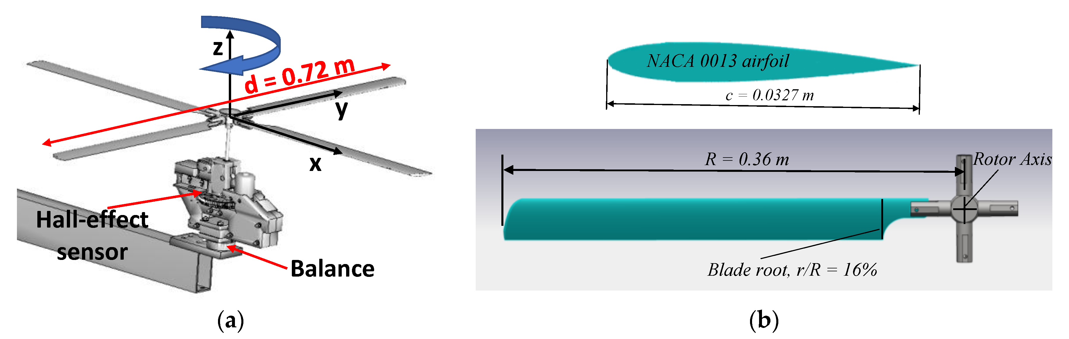
A dedicated rotor test rig was built based on an existing commercial radio-controlled helicopter model (Blade 450 3D RTF), (Figure 1a). The original two-bladed rotor was replaced by a four-bladed one with collective and cyclic control. The rotor blades were untwisted, with rectangular planform and parabolic tip. The blades presented a radius of and a chord length of . The root cut-out was located at 16% of the radius. A NACA0013 airfoil was used throughout the blade span. The blade planform and the geometry of the airfoil are shown in Figure 1b. The rotor solidity was equal to and the aspect ratio of the blades was . The rotor spun clockwise when seen from above, the collective pitch angle varied from to and the maximum speed was .
The force and moments produced by the rotor rig were measured by a six components balance (ATI MINI40). The detailed characteristics in terms of full scale and accuracy are summarized in Table 1.
The rotor test rig was located at a distance of 5 R from the floor and 3 R from the ceiling to avoid any influence of the surrounding walls. One hall-effect sensor was located on the shaft gear for measuring the rotating speed and for providing a trigger TTL signal at a prefixed azimuth angle to allow phase-locked measurements.
The current investigation addressed the wake downwash generated by the four-bladed rotor in hover conditions at a constant collective angle of . The angular velocity was set to , which leads to a blade tip velocity of Vtip = 66 m/s and a thrust value of T = 12 N. The resulting blade loading was with the density , and the rotor area A = 0.41 m2. The Mach and Reynolds numbers are given at the radius tip (Table 2).
2.1. PIV System and Evaluation
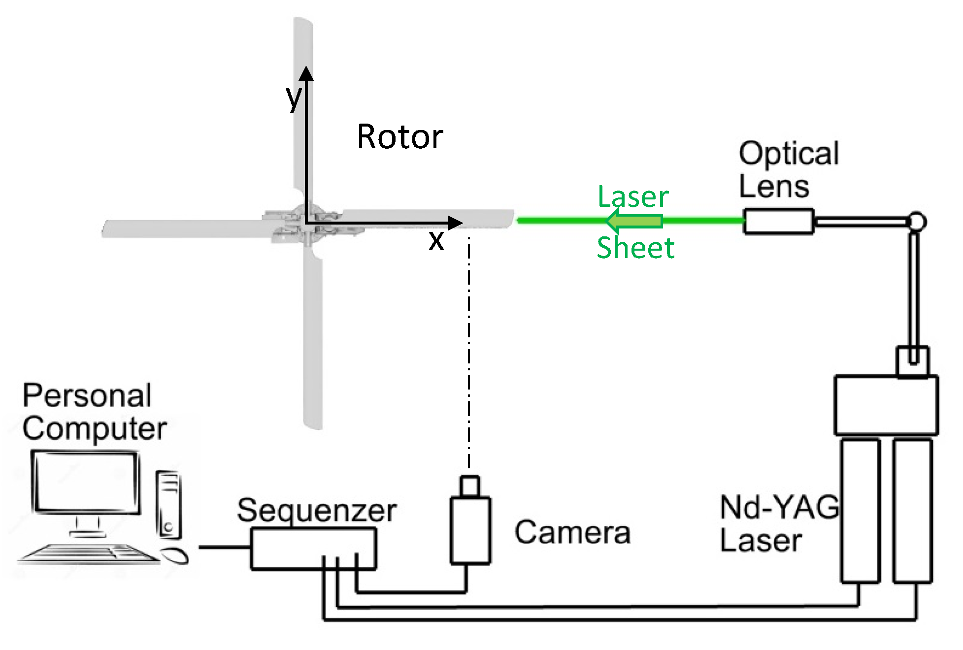
A fixed frame of reference was defined and having the origin located in the rotor centre with the x-axis horizontally oriented along the rotor blade, the y-axis orthogonal to the x-axis and lying in the rotor disk plane, and the z-axis vertically and upward directed. The rotor wake characteristics were investigated by a standard two-component PIV measurement system composed of a double head Nd-Yag laser with a maximum energy of 300 mJ per pulse at 532 nm and a single double frame CCD camera (2048 by 2048 px) with a dynamic range of 14 bits. The camera was mounted on two components translating system to cover the full region of interest in the xz-plane. The light sheet was vertically oriented and aligned with the rotor blade at the azimuth angle of Ψ = 180°. A standard PIV layout was adopted with the camera line of sight orthogonal to the laser sheet (Figure 2).
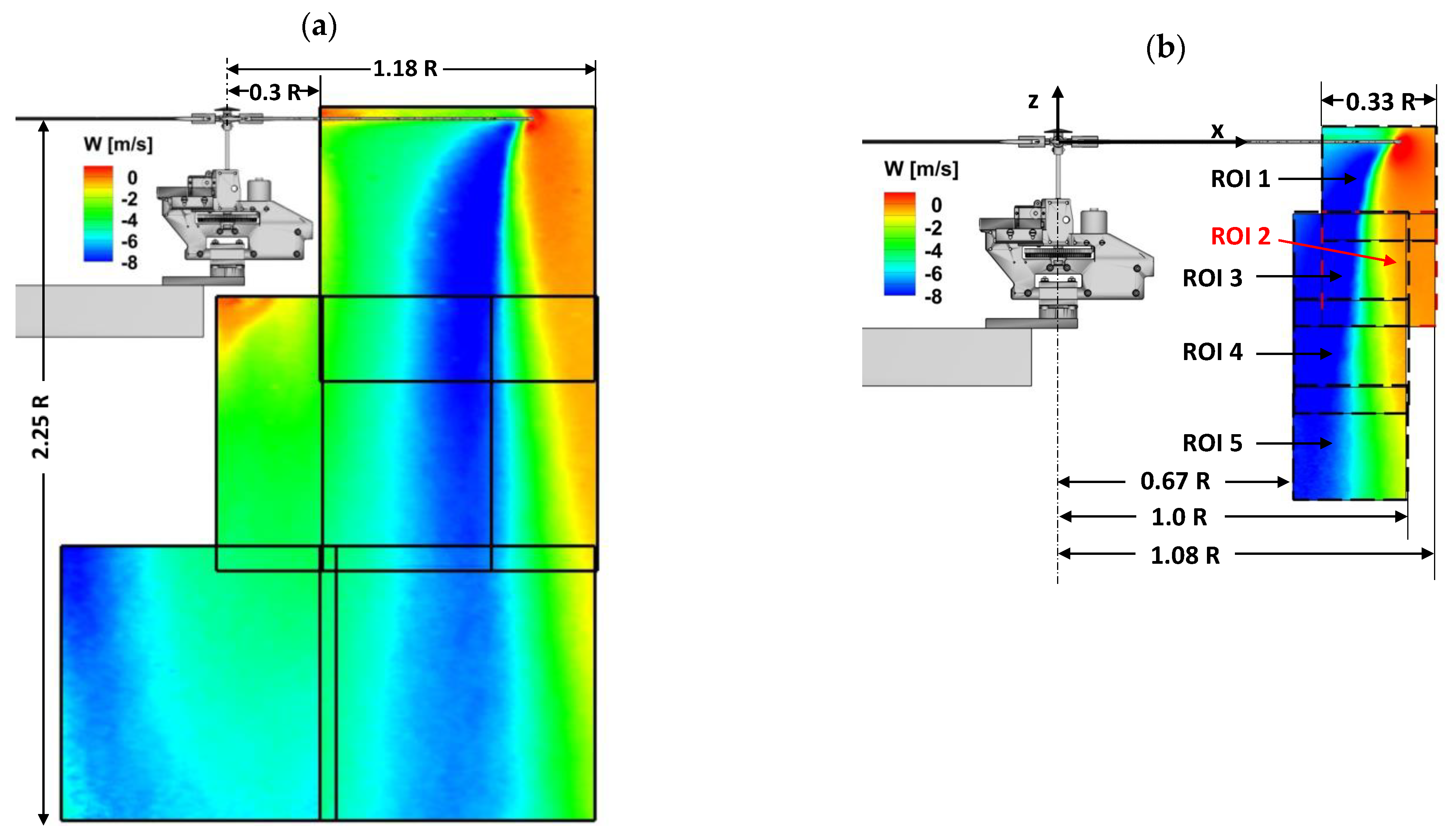
The wake downwash was investigated up to 2.25 rotor radii from the rotor disk. The camera, equipped with a 50 mm lens, recorded a measurement region of 320 mm by 320 mm, with a spatial resolution of 6 pixel/mm in the image plane. Separate measurement regions needed to cover the full wake (Figure 3a). The data post processing discussed in [16] provided a spatial resolution of not sufficient for the characterization of the tip vortices.
To track the blade tip vortices in proximity to the rotor disk, the camera was equipped with a lens featuring a fixed focal length of f = 200 mm, and the f-number was set to f# = 2.8. The measurement region was located immediately below the rotor disk plane on a vertical plane radially ranging between x/R = 0.68 and x/R = 1.08 to identify the trajectories of the trailing tip vortices. Five PIV measurement regions with the size of about 120 mm by 120 mm, partially overlapped, were used to measure the rotor wake, and in particular the blade tip vortices characteristics up to one radius downstream the rotor disc, Figure 3b. This yielded a spatial resolution of about 17 px/mm in the image plane. The delay time between the two laser pulses was set to 25 μs according to the highest expected velocities in the flow. As tracer particles, sprayed diethylhexylsebacate (DEHS) oil was used. A seeding generator with 20 Laskin nozzles provided oil droplets with an average size less than 1 μm. The full test room was seeded to have a homogenous concentration of particles. More than 150 image pairs were recorded at a frame rate of 3 Hz for each region of interest (ROI) over about 1450 rotor revolutions. The PIV images were pre-processed by applying a background grey-level subtraction. PIV-View 3.60 was used to process the images. The analysis consisted in a Multi-grid scheme with a B-Spline of 3rd order image deformation ending at 32 × 32 px2 and 75% overlap. Correlation maps were calculated by FFT multiple correlations (Hart [25]) of 2 windows and a 3-point Gaussian peak fit was used to obtain the displacement.
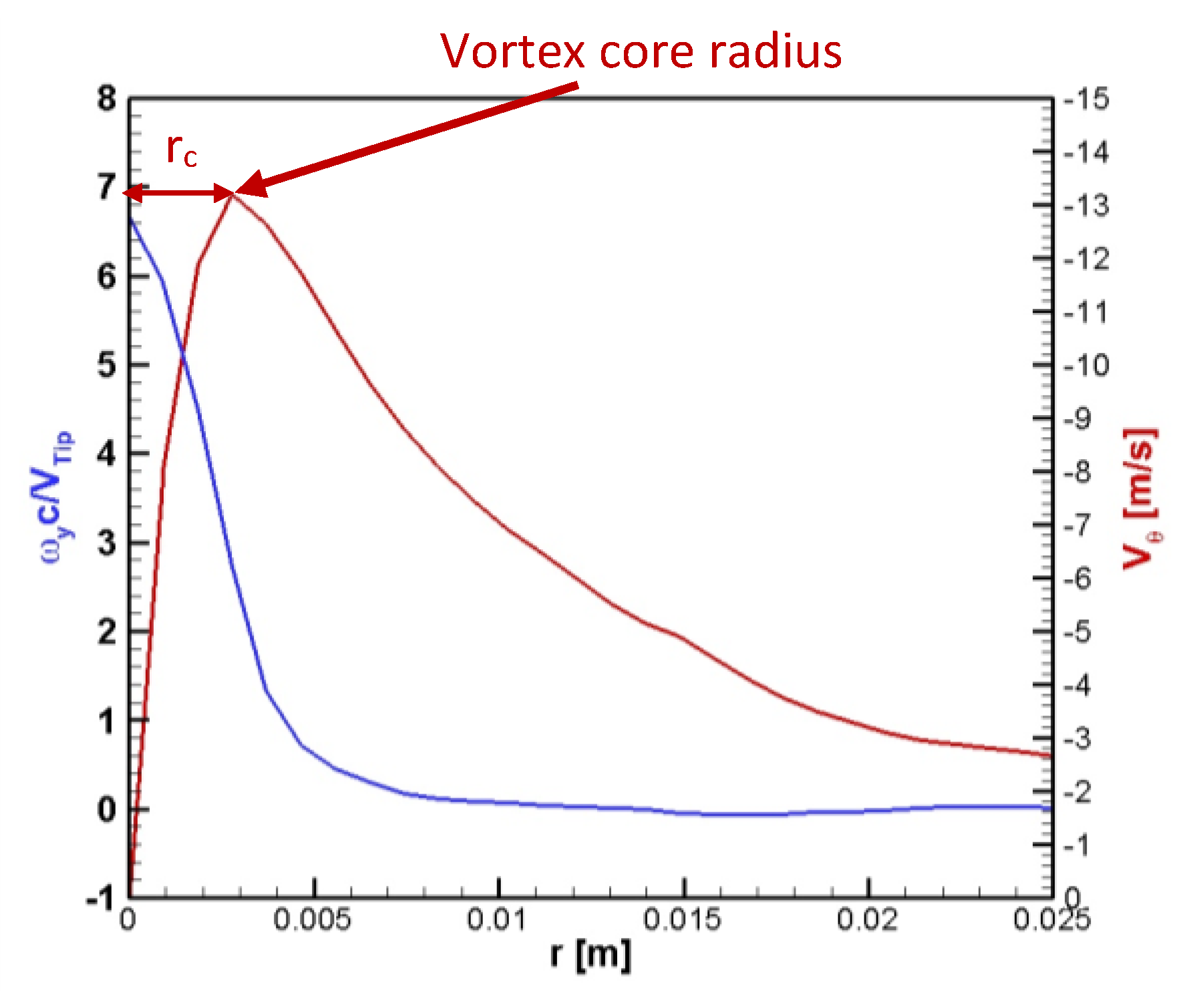
The results presented a velocity spatial resolution of . The random noise of the PIV cross-correlation procedure can be estimated as 0.1 px as a rule–of–thumb (Raffel et al. [26]). Using the current values for the optical resolution (17 px/mm) and the laser double–pulse delay (25 μs), this leads to a velocity error of of for the PIV measurements. In the proximity to the rotor disk, the core radius rc of the tip vortices was measured. The core radius is defined as the distance from the vortex centre to the radial position where the maximum swirl velocity is reached (Figure 4). Values of rc between 3 and 3.3 mm were measured giving a ratio of about 0.15–0.14 according to the value of indicated by Martin et al. [1] to guarantee a correct vortex characterization.
2.2. Vortex-Identification Criterion
To overcome the difficulty in identifying the centre of the vortices in the presence of spurious vectors, a method based on the velocity field topology, without using velocity derivatives was chosen. This was the -criterion proposed by Graftieaux et al. [22]. The function is defined in discrete form as:
with representing a two-dimensional circle around with radius D, the number of grid points inside with umean the average velocity vector within the region S, the unit vector normal to the PIV plane and the velocity at . The l radius of the domain is expressed in terms of grid spacing. is a 3D non-dimensional scalar function, with . The zones delimited by identify the vortices present in the measurement region. The vortex centre is identified as the maximum value of the absolute of in the delimited zone. In cases of PIV data affected by spurious vectors or data void, it is suggested to use the weighted centroid of the for the identification of the centre of the vortex. In the current work, the weighted centroid is chosen to identify the centres. The choice of the domain radius influences the accuracy of the centre detection and the dimension of the identified vortices. De Gregorio and Visingardi [27] indicated that the selection of a domain radius , equal to the larger core radius existing within the investigated flow field, provides the best measurement accuracy for single and multiple vortices affected by spurious vectors. In the case of elliptical vortices, a domain radius equal to the semi-major axis is recommended for reducing centre detection errors, whereas the magnitude of the domain radius is recommended to be set between two to six times the core radius size in the case of significant data void in the vortex core.
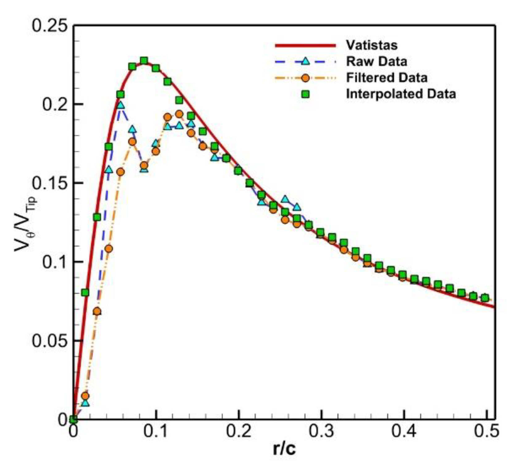
In the processing of the PIV images, the lack of particles caused a number of spurious velocity vectors. A normalised median test, presented by Westerweel and Scarano [28], coupled to a Dynamic Mean Test and a Global Histogram Filter (described by Raffel et al. [26]) were used to detect and then remove the spurious vectors. After deleting the outliers, the missing data were replaced using bi-linear interpolation. Taking into account the particle void, the domain radius D was fixed equal to 10 grid spacing, which was almost twice the value of the vortex core radius ( grid point as shown in Figure 5). Once the centre was detected, the vortex characteristics were calculated on concentric circles moving away from the centre. The raw or filtered data have shown scattering data in the core, while the interpolated data provided a satisfactory agreement with the Vatistas [29] theoretical curve (Figure 5). The agreement between the linear interpolated data and the Vatistas vortex is explained by the nature of a real vortex core where the tangential velocity behaviour is linear and can be expressed as , thus justifying the application of a bi-linear interpolation to account for the missing vectors.
3. Numerical Methodology
The numerical simulations were carried out by using the code RAMSYS [30], which is an unsteady, inviscid and incompressible free-wake vortex lattice Boundary Element Method (BEM) solver for multi-rotor, multi-body configurations developed at CIRA. It is based on Morino’s boundary integral formulation for the solution of the Laplace equation for the velocity potential [31].
3.1. Governing Equation
The fluid is assumed to be inviscid, incompressible and irrotational. Under these hypotheses there exists a function , called velocity potential, such that the velocity vector and the continuity equation reduces to Laplace equation:
The application of the Green’s function to Equation (2) yields a boundary integral representation of the velocity potential:
where and are body and wake surfaces, respectively, and is the free-space fundamental solution of the 3D Laplace equation.
3.2. Boundary Conditions
Far from the body, the velocity potential is null at infinity:
The impermeability boundary condition on yields:
where denotes the velocity of body points and denotes the outward unit normal vector on .
The boundary condition on the wake is expressed as:
according to which the potential jump across the wake surface is constant:
with denoting the time taken by the wake material point to move from the trailing edge to its current position.
3.3. Novel Boundary Integral Formulation
The novel formulation proposed by Gennaretti et al. [32] is applied in RAMSYS to avoid the instabilities arising in the numerical formulation when wake panels are too close to or impinge the body. In this formulation, the velocity potential is split into a scattered potential , generated by sources and doublets over and doublets over the part of the wake surface in contact with the blade trailing edge (Near wake, ), and an incident potential , generated by doublets over the part of the wake not in contact with the trailing edge (Far wake, ), such that and .
The application of this novel formulation provides a new expression of Equation (3), which is then replaced by:
and by:
where the boundary conditions are given by:
and:
with the velocity induced by the far wake obtained from the gradient of Equation (9) combined with Equation (11),
3.4. Numerical Solution
The numerical solution of Equation (8) is obtained by defining boundary elements, i.e., by discretizing and into quadrilateral panels, assuming , , to be piecewise constant, and imposing that the equation is satisfied at the centre of each body element (collocation method). Specifically, dividing the blade surface into M panels, , and the wake surface into N panels, , the discretized version of Equation (8) gives the linear algebraic system:
where , , whereas source/sink and doublet coefficients are given by:
The solution of the algebraic system is obtained by the application of the GMRES iterative method.
Once the potential field is known, the surface pressure distributions are evaluated by applying the unsteady version of the Bernoulli equation:
where the incident potential is obtained from integration of the incident velocity field by using Equation (12) with the inclusion of the vortex-core model. Finally, the evaluation of the forces and moments is obtained by the integration of Equation (15).
3.5. Vortex Core Model
To account for the viscous diffusion of the wake vortex elements, the Vatistas vortex core model was used, according to which the swirl velocity is expressed as:
where the coefficient has been set equal to “1”, as suggested by Scully [33].
The applied diffusion model is the one described by Squire [34]. In this model, the growth with the time of the core radius is given by:
where the term is the initial core radius that removes the singularity at , and was set equal to 5% of the blade average chord length c in the calculations, the term α is the Oseen coefficient and is equal to 1.25643. The product δv represents the “eddy viscosity” where v is the kinematic viscosity and:
represents an average effective (turbulent) viscosity coefficient in which is the circulation strength of the vortex element, while the Squire’s coefficient is an empirical parameter specified to vary between 0.2 and 0.0002, as indicated in Bhagwat [35]. For a small-scale rotor, like the one used for these investigations, a value of can be used. The model suggested by Donaldson & Bilanin [36] was used to take into account the decay of the circulation with time. According to this model, the circulation of the tip vortex is expressed as:
being a decay coefficient; the ambient turbulence level and the aircraft semispan. In the present calculations, the coefficient was replaced with a single coefficient set equal to 2.5. This value was tuned, together with the empirical parameter finally set to 0.0003, to match several experimental observations [35,37,38] according to which the effective diffusion Squire/Lamb constant for small scale helicopter rotors.
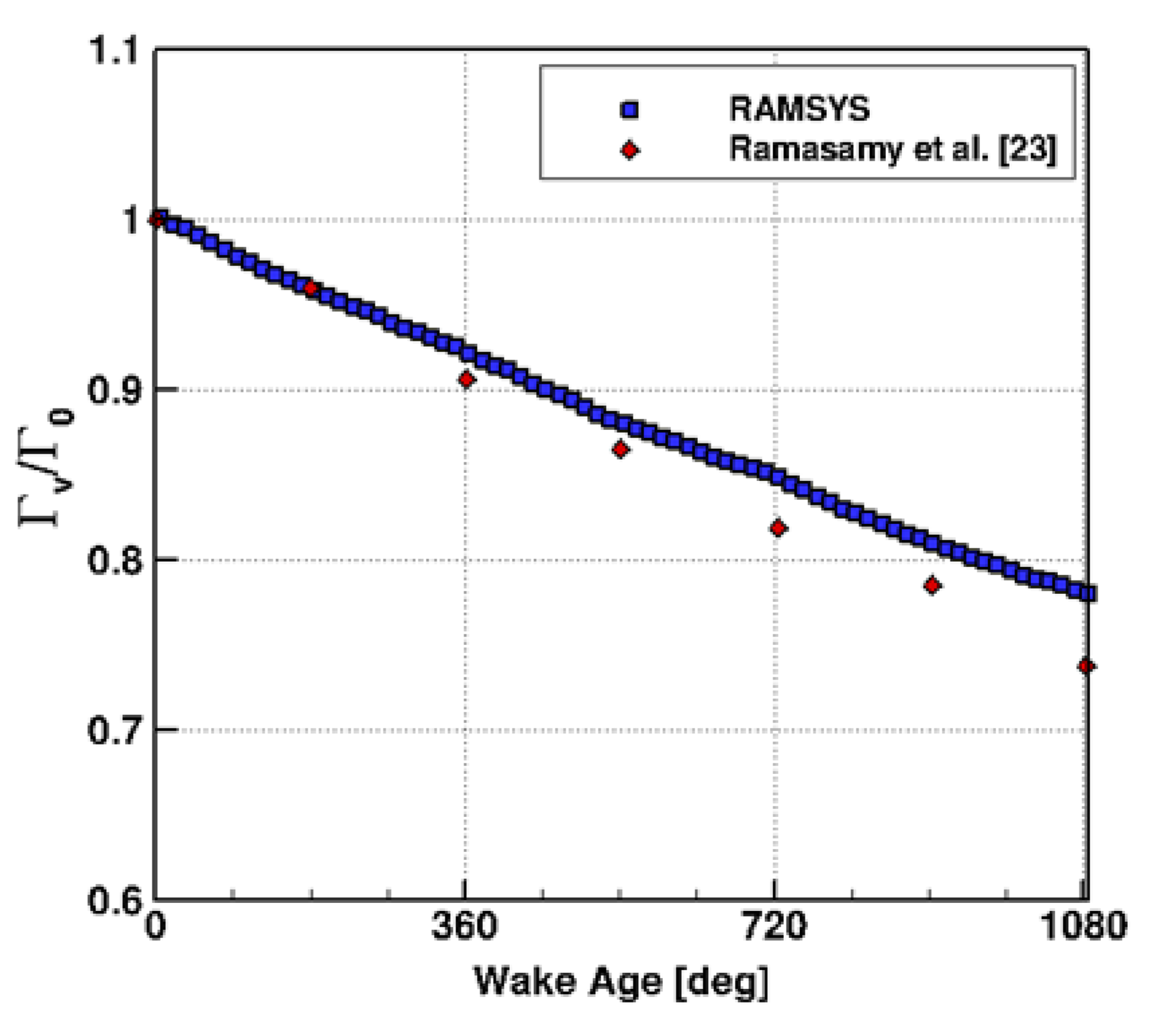
Figure 6 illustrates the decay of the normalized vortex circulation with the wake age obtained by applying the decay model of Equation (9) and using the value of 2.5 for the decay coefficient. Despite the slope is slightly lower than the measurements reported in Ramasamy et al. [37], a good agreement with the experimental results can be observed.
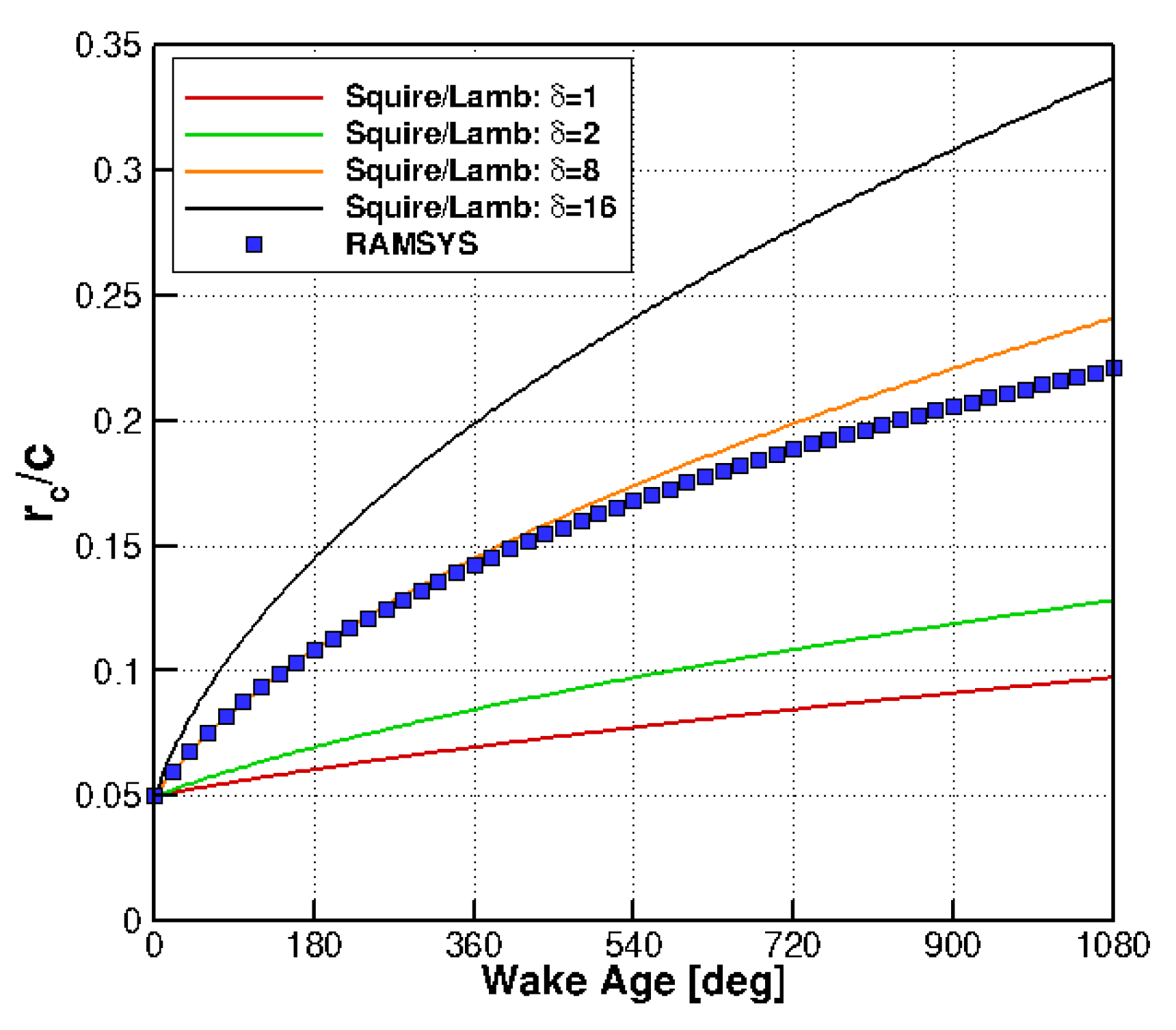
Figure 7 shows the predicted growth of the vortex core radius as a function of the wake age obtained by applying Equation (17) and using Equation (18) for the diffusion parameter and Equation (19) for the circulation decay. The picture highlights the close agreement of the calculated parameter with the constant value of 8, which is typical for small scale helicopter rotors. The slight increasing deviation with the wake age from the value of 8 is produced by the application of the decay model in the vortex circulation.
4. Results
PIV measurements and BEM numerical simulations were carried out with the main purpose to investigate the structure and development of the rotor blade tip vortices.
4.1. Numerical Test Set-Up and Computational Resources
Each of the four-rotor blades was discretized by 40 chordwise panels and 23 spanwise panels. No rotor hub nor any other body (such as the motor, the controller, etc.) was modelled. Fourteen rotor revolutions and fourteen wake spirals were required to get a sufficiently long wake and a converged solution. The time discretization adopted corresponded to an azimuth step equal to 2 deg. A computational acceleration was obtained by running the code in parallel mode via the OpenMP API and using 32 cores. The run required about 8 h of elapsed computational time.
4.2. Rotor Wake Ensemble-Averaged Flow Field
The ensemble-averaged velocity field showed the shear layer region surrounding the rotor downwash wake.
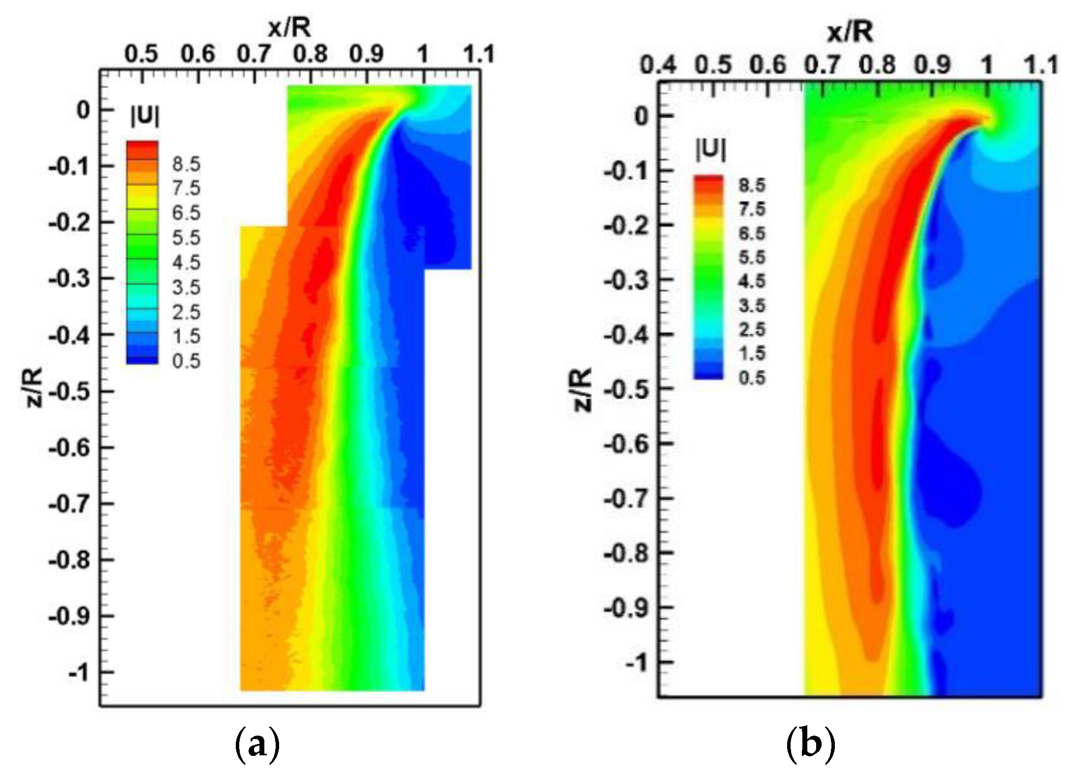
The comparison between the experimental results, Figure 8a, and the numerical predictions, Figure 8b highlighted a general similarity but with two main differences:
- in the experimental PIV the origin of the shear layer is identified at about x/R = 0.96 and slightly above z/R = 0 because of the deflection produced by the blade elasticity. Instead, the numerical results show the origin of the shear layer exactly at x/R = 1 and z/R = 0, and this is because the blade was modelled as a fully rigid body;
- the diffusion produced by the viscous effects causes a marked thickening of the experimental shear layer moving downstream from the rotor disk, while the dissipation produces a reduction of the velocity magnitude which is already visible at around z/R = −0.7. These effects are less visible in the numerical results, despite diffusion and dissipation models were applied in the simulations.
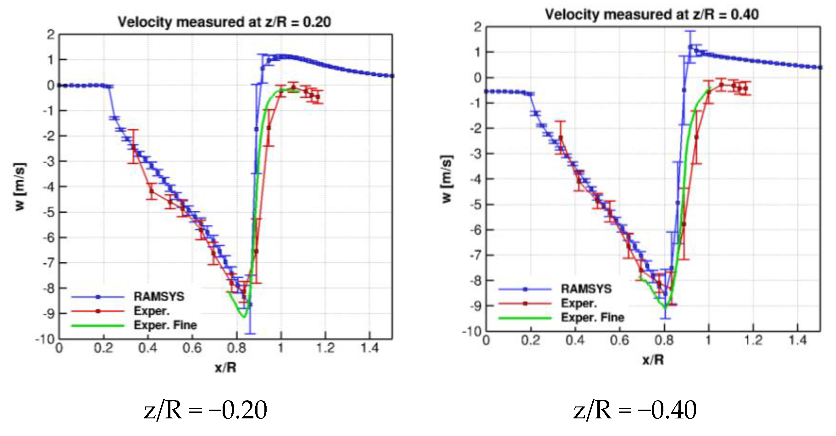
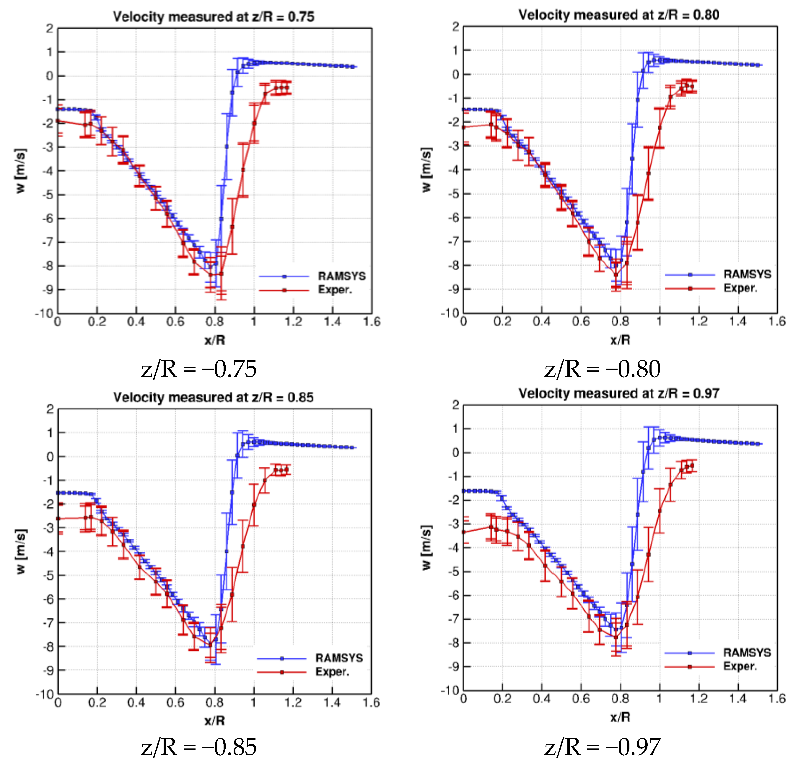
A deeper investigation of the aforementioned differences was obtained by comparing the experimental and numerical z component of the induced velocity at several stations below the rotor disk in a region extending up to one radius below the rotor, Figure 9. The numerical results shown in the figure were evaluated at the several azimuthal stations of the last rotor revolution and time-averaged, whereas the velocity fluctuations, due to the flow field unsteadiness, was evaluated and represented in terms of RMS bars. The experimental PIV measurements were made in a fixed vertical plane during about 1450 rotor revolutions. The values were then ensemble-averaged and the velocity fluctuations were represented in terms of RMS bars.
The numerical predictions show a satisfactory agreement with the experiment in the radial region of the blade included from the root cut-out (16%) to the position , where the maximum of the inflow is measured. In the radial region, where the tip vortex roll-up produces its greater effect, the numerical results show an upwash that is not present in the experiment. Furthermore, discrepancies between the numerical results and the experiment can also be observed in the region of the rotor hub, not modelled in the numerical simulations.
Finally, the different slope of the derivative between the experiment and the numerical simulation around 80–100% of the blade radius was further analysed by comparing the PIV measurements made with a finer resolution (), with those at a resolution of () and with the numerical results evaluated on a grid having a resolution of . The results showed that the slope evaluated by the finer PIV measurements are much closer to the numerical results but this happens up to z/R = 0.4. More downstream, the slope of the finer and coarser PIVs remains almost unchanged.
4.3. Blade Tip Vortices
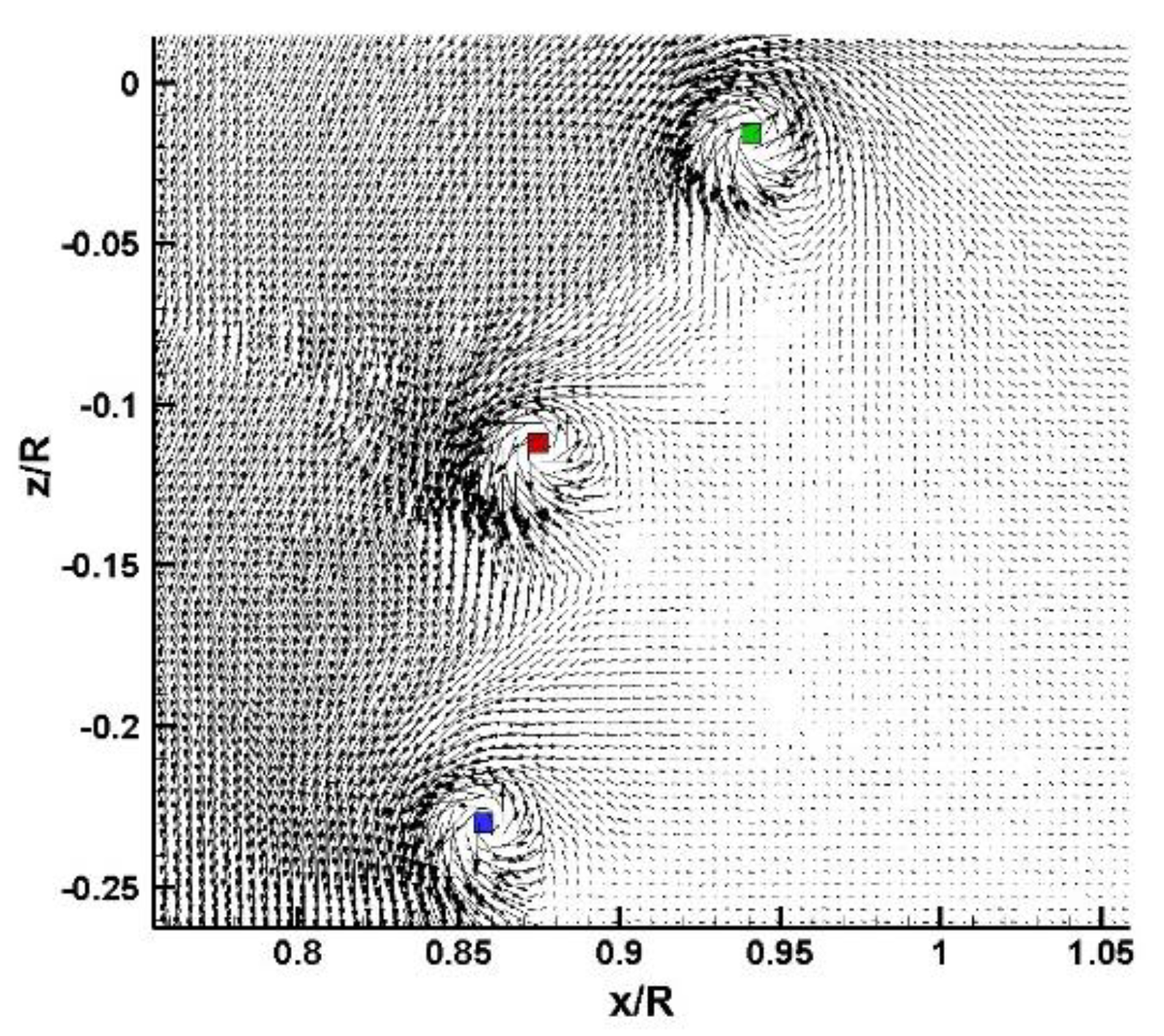
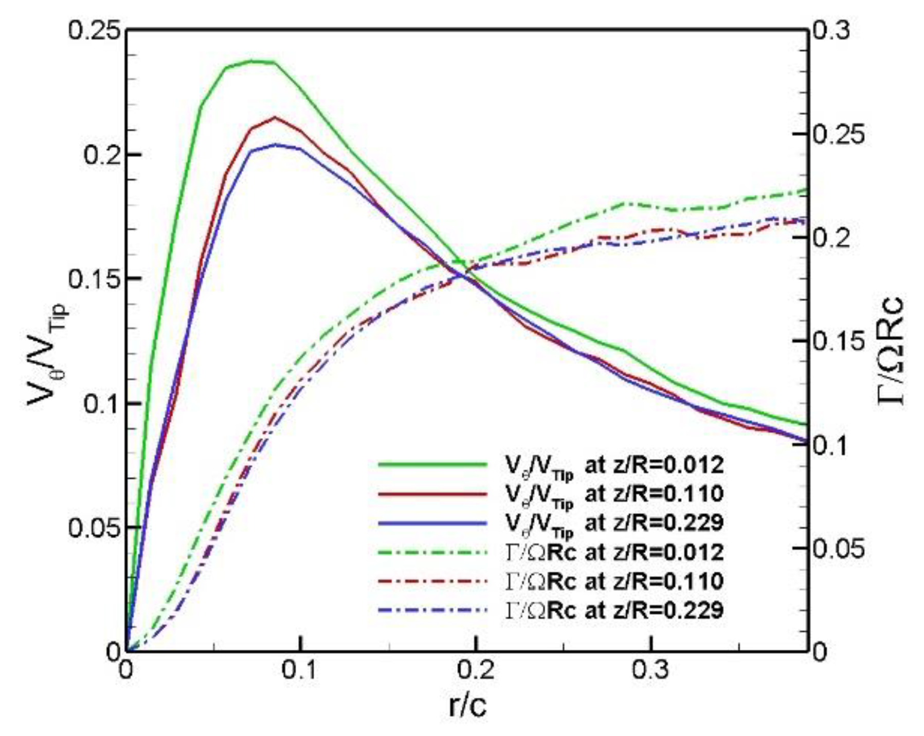
The application of the method to the PIV and BEM instantaneous velocity fields highlighted the presence of several tip vortices in the measurement regions. Figure 10 shows an instantaneous velocity field in the ROI immediately downstream of the rotor disc. Three tip vortices can be counted and the vortex centres detected by method are shown. Once the centres of the tip vortices were detected, the non-dimensional tangential velocities and circulations were calculated and represented versus the non-dimensional vortex radius (Figure 11).
The results have shown a decrement of the swirl velocity that follows a second-order trend as the distance from the rotor increases. The circulation decreases as the distance from the disk increases.
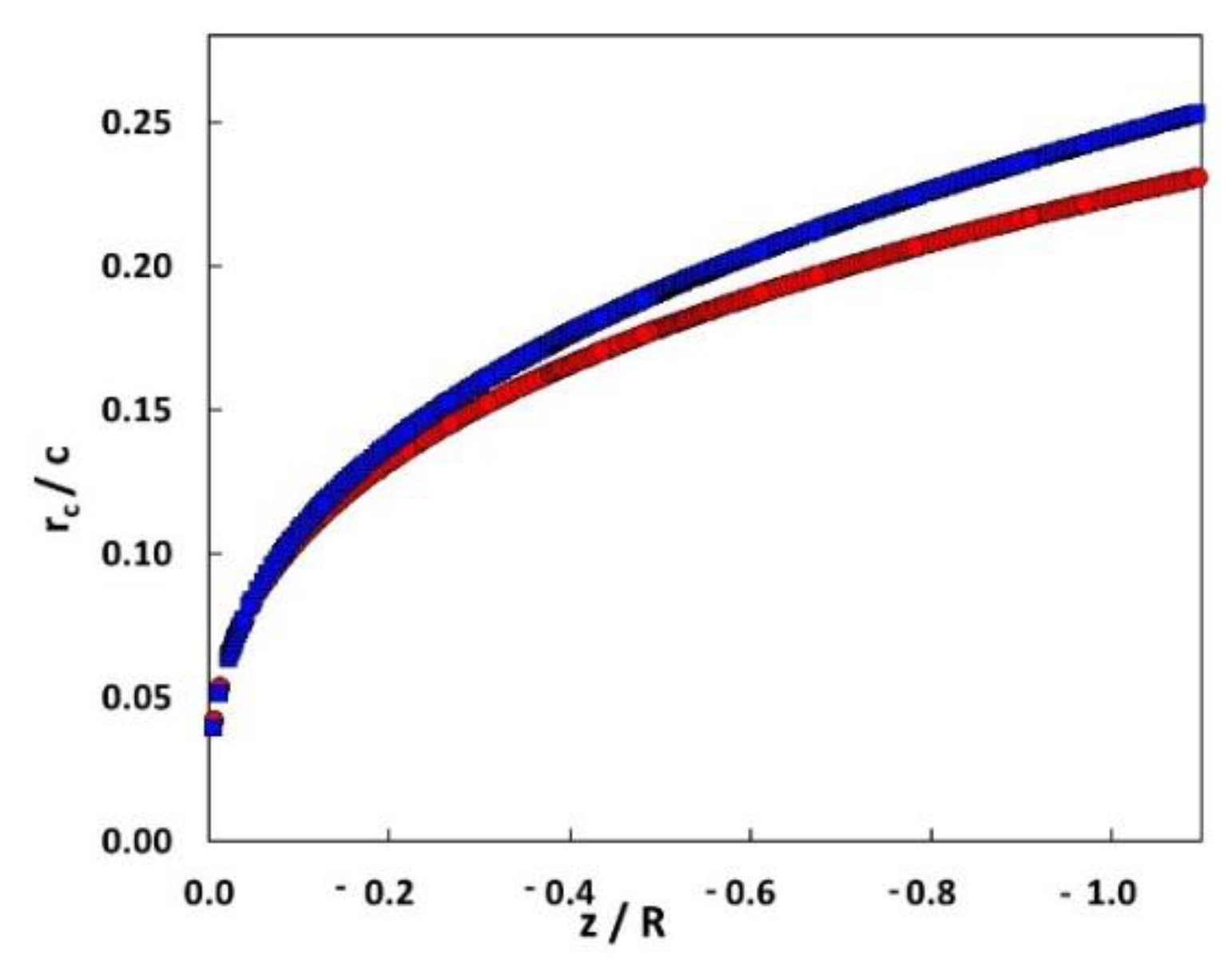
The PIV measurements were not phase-locked with the rotor so that a direct comparison between instantaneous velocity fields was not possible. The BEM/PIV comparison was carried out on the tip vortex characteristics versus the distance from the rotor disk. The growth of the normalized vortex core radius with the distance from the rotor disk is shown in Figure 12. The comparison between the experimental and numerical results show that in the latter case the growth is slightly over-estimated.
The distribution of the experimental vortex centres, Figure 13, showed the highest concentration in the proximity to the rotor disk and that their location was enclosed in the shear layer region. Moving downstream, the data scattering increased distributing the centres of the vortical structures both outside and inside the ensemble-averaged downwash, whereas the concentration of vortex decreased due to the fading and/or merging of vortices. The same representation for the numerical vortex centres showed an extremely narrow region of the shear layer and an almost full match between the boundaries of the shear layer region and the path of the vortex centres.
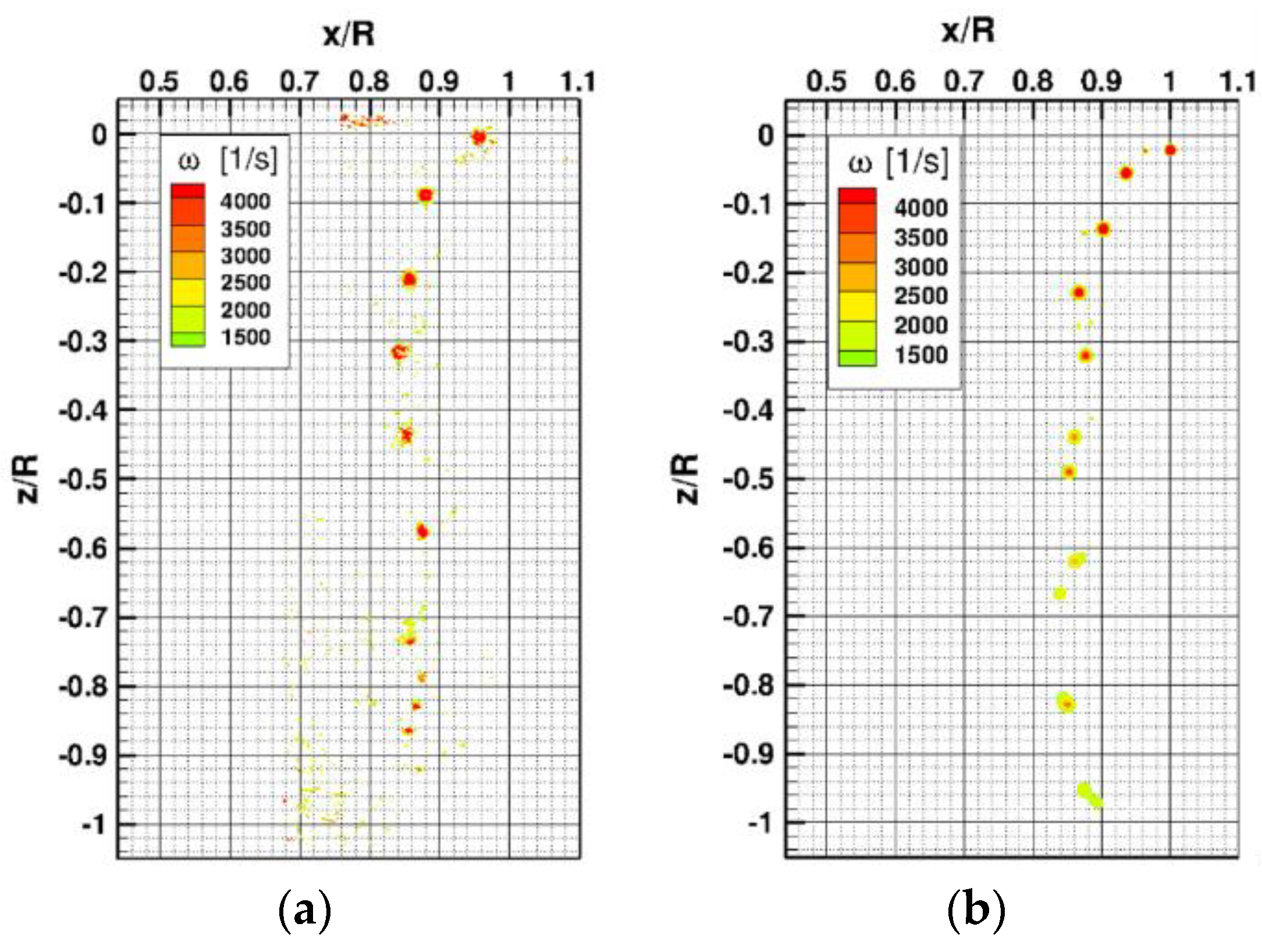
Additional characterization of the instantaneous tip vortices was obtained by evaluating the composition of the vorticity orthogonal to the PIV plane and comparing the experimental results with the numerical simulations. Figure 14 illustrates the results of this comparison. A cut-off of the vorticity module was set at 1500 to remove as much as possible the flow field small-scale turbulence and to have a more concentrated representation of the tip vortices. PIV results generally show stronger vorticity. The blade flexibility in the experiment generates the tip vortex at a higher and more inboard position with respect to the BEM result (. The presence of widespread vorticity along the blade span around x/R = 0.8 and z/R = 0 can be observed in the PIV due to the blade passage.
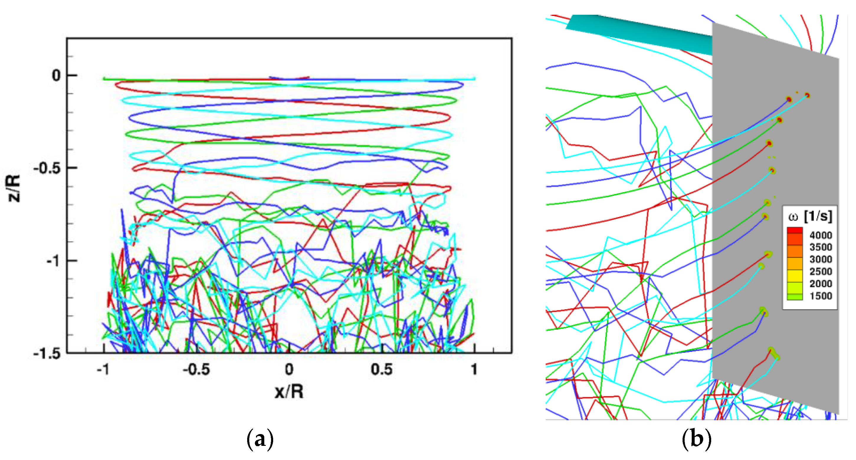
The numerical simulations allowed the visualization of the entire wake structure generated by the rotor. In particular, it was possible to visualize the tip vortices and to associate them with the generating blades. Figure 15a shows the numerical tip vortex structure up to a distance of z = −1.5 R below the rotor disk. Each of the four colours corresponds to a vortex filament generated by the relative blade. The image illustrates that the vortex structure keeps a geometrical regularity until a distance between z/R = −0.5 and −0.6, after which the wake starts showing more chaotic behaviour. A second aspect that is highlighted in the figure is the pairing phenomenon according to which the mutual positions of the vortex filaments tend to interchange after a first rotor revolution. More specifically, looking at the sequence of the tip vortices at about x/R = + 1.0, it is: cyan-blue-green-red during the first revolution but becomes cyan-green-blue-red during the second revolution. This means that the vortices blue and green begin to roll up with each other until when they have completely interchanged their position after one revolution. Analogously, similar behaviour can be observed at about x/R = −1.0, for the vortex filaments red and cyan. This mechanism contributes to increasing the flow turbulence from the third revolution onward.
Figure 15b shows the association between the numerical vortex filaments and the generated vorticity in the plane corresponding to the PIV measurements. The pairing phenomenon is clearly visible after the second revolution between the green and blue vortex filaments, highlighted in the figure by the black circle, with the vorticity intensity of the first one being smaller than that of the second one. The dashed black circle shows that during the third revolution the green and blue vortex filaments tend to coalesce.
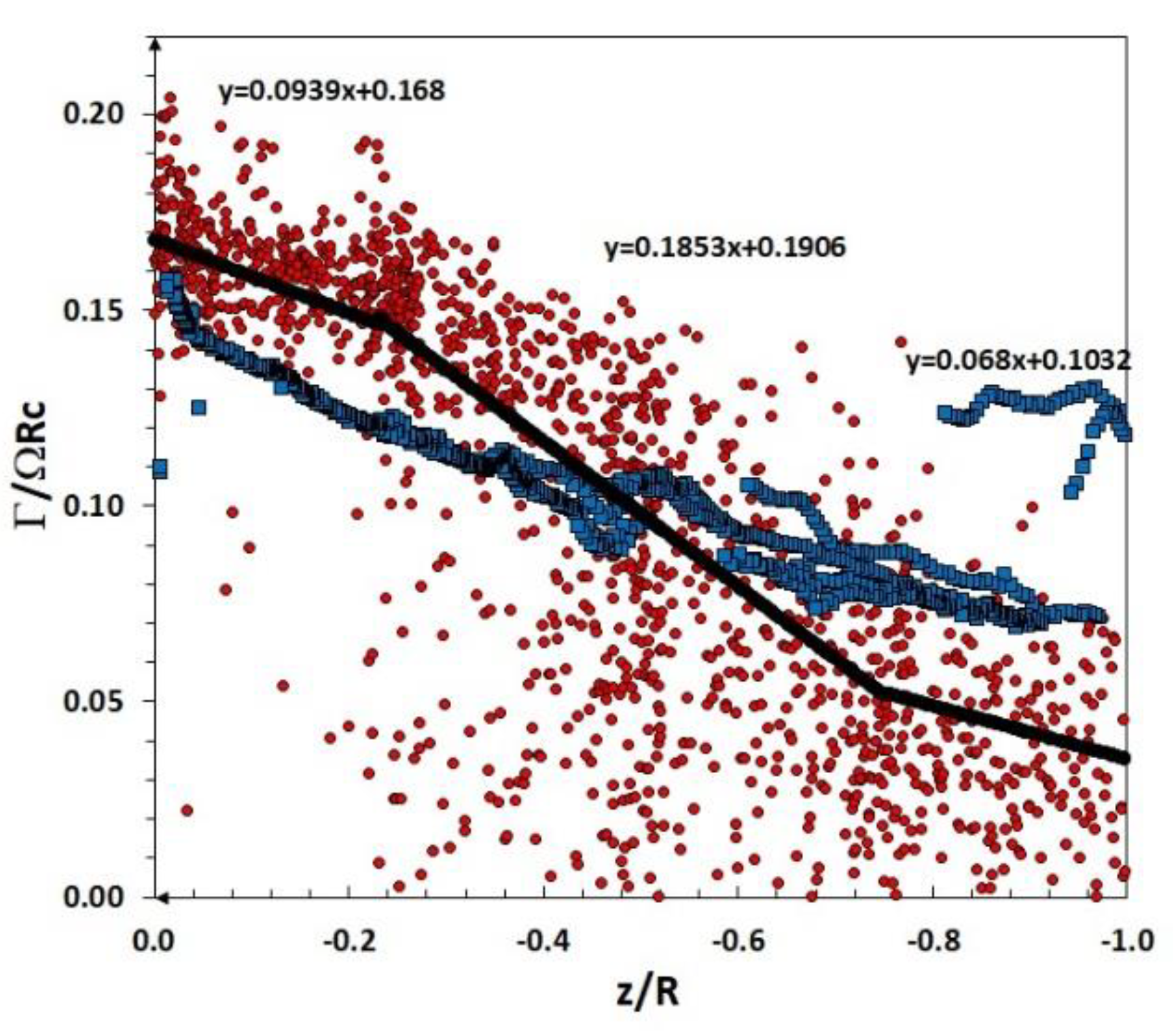
Figure 16 shows a comparison between the experiment and the numerical simulation in terms of the variation of the non-dimensional net circulation of all the identified tip vortices versus the distance from the rotor disk z/R. The net circulation was determined at a distance of 0.25 c from the vortex centre, and by assuming axisymmetric flow in the reference system moving with the vortex core, following the specification in Ramasamy et al. [37]. The experimental data presents three different regions characterised by different slopes, a near-field region comprised between the rotor disk to z/R = −0.23, a mid-region with z/R ranging between −0.23 and −0.75 and a far-field region from z/R = −0.75 to −1.1. In the near-field region, the experimental/numerical comparison shows a reasonable agreement in terms of slope, while an intensity difference of about 17% arises. In the mid-region, where the pairing phenomena start to occur (z/R = −0.5), the experimental slope is almost doubled with respect to the near-field region, and the intensity dissipation is larger than the numerical data. Further downstream, the experimental slope realigns to the numerical trend but with smaller values.
The change in slope of the experimental data in the mid-region and their subsequent scattering at distances z/R < −0.25 might be explained by an increase in dissipation due to the growing of turbulence and by the process of pairing and coalescence of vortex filaments, respectively. This process was also mentioned in the explanation of the BEM tip vortices path of Figure 15a. The numerical results resemble the trends illustrated in Figure 6. The merging of co-rotating vortices, which produce a higher circulation, likely causes the presence of higher values in the region .
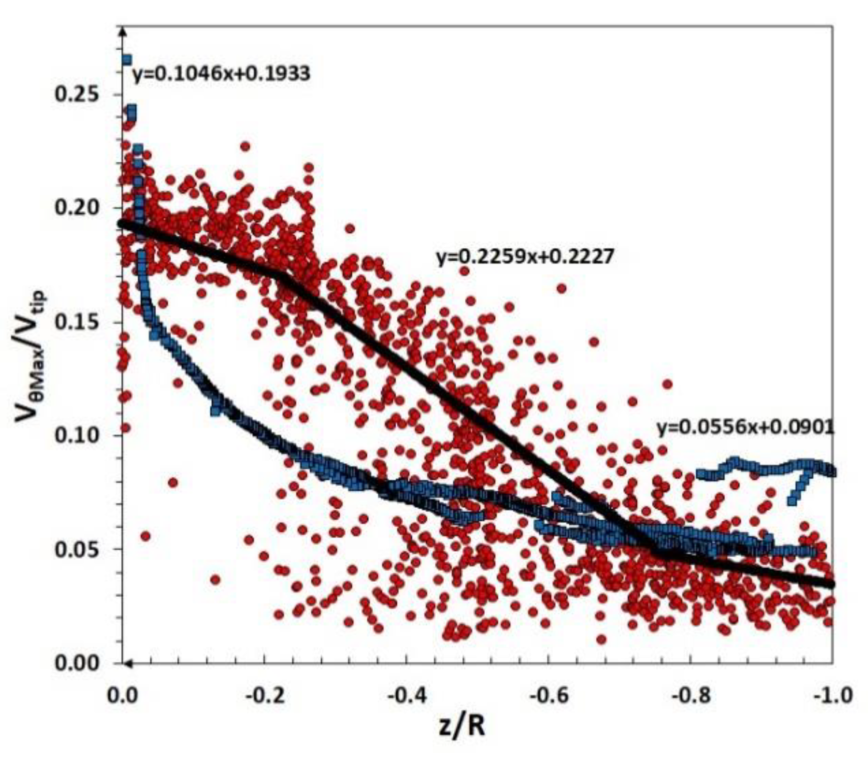
Finally, Figure 17 shows a comparison between the experiment and the numerical simulation in terms of the maximum values of the non-dimensional swirl velocity of all the identified tip vortices versus the distance z/R. In this case, the experimental vortices also show three distinct zones with a net difference in terms of slopes and intensities. The reason for this behaviour has the same explanation as for the net circulation trend discussed in Figure 16. The numerical results show a typical hyperbolical decay of the velocity intensity according to the model of Equation (16) combined with Equation (17). An interesting match with the experiment can be observed for distances from the rotor disk lower than z/R = −0.5. The presence of higher values in the region z/R ∈ [−0.8; −1.0] is likely caused by the merging of co-rotating vortices which produce a higher velocity swirl, as also mentioned for the net circulation.
5. Conclusions
Research activity was carried out to characterize experimentally and numerically the blade tip vortices of a small scale four-bladed isolated rotor in hover flight. The investigation of the vortex decay process during the downstream convection of the wake was addressed. 2C-2D PIV measurements were carried out below the rotor disk down to a distance of one rotor radius. The numerical simulations were aimed at assessing the modelling capabilities and the accuracy of a free-wake Boundary Element Methodology.
The Γ2 vortex centre detection criterion was applied both to the experimental and numerical results. Once detected in the centres, tip vortices were characterised in terms of vorticity, circulation, swirl velocity, core radius and trajectory.
The rotor wake mean velocity field and the instantaneous vortex characteristics were investigated. The experimental/numerical comparisons showed a reasonable agreement in the estimation of the mean velocity inside the rotor wake, whereas the BEM simulations predicted and under-estimated the effect of the diffusion thus generating a smaller shear layer region with respect to the experiment.
The numerical results provide a clear picture of the filament vortex trajectory interested in complex interaction starting at about a distance of z/R = −0.5.
The time evolution of the tip vortices was investigated in terms of net circulation and swirl velocity. The PIV results showed similar behaviour for both quantities. They showed a linear mild decay up to the region interested by vortex pairing and coalescence, where a sudden decrease, characterised by a large data scattering, occurred. The numerical modelling predicted a hyperbolic decay of the swirl velocity down to z/R = −0.4 followed by an almost constant decay. Conversely, the calculated net circulation showed a gradual decrease throughout the whole wake development.
The comparisons showed discrepancies in the region immediately downstream the rotor disk but significant similarities beyond z/R = −0.5.
Author Contributions
Conceptualization, F.D.G.; methodology, F.D.G. and A.V.; software, A.V.; validation, F.D.G. and A.V.; formal analysis, F.D.G. and A.V.; investigation, F.D.G.; resources, F.D.G. and A.V.; data curation, F.D.G., A.V., and G.I.; writing—original draft preparation, F.D.G.; writing—review and editing, F.D.G., A.V., and G.I.; visualization, F.D.G. and A.V.; supervision, F.D.G.; project administration, F.D.G.; funding acquisition, F.D.G. All authors have read and agreed to the published version of the manuscript.
Funding
This research received no external funding.
Institutional Review Board Statement
Not applicable.
Informed Consent Statement
Not applicable.
Conflicts of Interest
The authors declare no conflict of interest.
Abbreviations
The following nomenclature and abbreviations are used in this manuscript:
| AR | blade aspect ratio |
| c | blade chord [m] |
| CT | thrust coefficient = T/(ρπR2Ω2R2) |
| D | Γ2 domain radius |
| Ktip | reduced frequency |
| Mtip | tip Mach number |
| Nb | number of blades |
| r | local blade radius [m] |
| rc | vortex core radius [m] |
| R | rotor radius [m] |
| Retip | tip Reynolds number |
| t | time [s] |
| T | rotor thrust [N] |
| |U| | modulus of the induced velocity [m/s] |
| v | induced velocity [m/s] |
| VB | local tangential velocity = Ω r [m/s] |
| Vtip | velocity at blade tip [m/s] |
| Vθ | swirl velocity [m/s] |
| w | axial induced velocity component [m/s] |
| x | spanwise distance [m] |
| z | axial distance from the rotor disk [m] |
| Γ, Γv | tip vortex circulation [m2/s] |
| Γ2 | vortex detection scalar value |
| Γ0 | tip vortex circulation at t = 0 [m2/s] |
| Γ2 | vortex detection scalar value, [-] |
| δ | eddy viscosity [m2/s] |
| θ0 | blade collective pitch [deg] |
| ν | kinematic viscosity [m2/s] |
| ρ | air density [kg/m3] |
| σ | rotor solidity |
| φ | velocity potential [m2/s] |
| Ψ | rotor azimuth angle |
| ω | out-of-plane vorticity [1/s] |
| Ω | rotor speed [rad/s] |
| BEM | Boundary Element Method |
| CIRA | Centro Italiano Ricerche Aerospaziali |
| PIV | Particle Image Velocimetry |
| TE | Trailing-Edge |
| RMS | Root Mean Square |
| W | Wake |
References
- Martin, P.B.; Pugliese, G.J.; Leishman, J.G.; Anderson, S.L. Stereo PIV measurement in the wake of a hovering rotor. In Proceedings of the 56th Annual Forum of the American Helicopter Society, Virginia Beach, VA, USA, 2–4 May 2000. [Google Scholar]
- Heineck, J.T.; Yamauchi, G.K.; Wadcock, A.J.; Lorenco, L.; Abrego, A. Application of three-component PIV to a hovering rotor wake. In Proceedings of the 56th Annual Forum of the American Helicopter Society, Virginia Beach, VA, USA, 2–4 May 2000. [Google Scholar]
- McAlister, K.W. Rotor Wake Development during the First Revolution. J. Am. Helicopter Soc. 2004, 49, 371–390. [Google Scholar] [CrossRef] [Green Version]
- Richard, H.; van der Wall, B.G. Detailed Investigation of Rotor Blade Tip Vortex in Hover Condition by 2C and 3C-PIV. In Proceedings of the 32nd European Rotorcraft Forum, Maastricht, The Netherlands, 12–14 September 2006. [Google Scholar]
- De Gregorio, F.; Pengel, K.; Kindler, K. A comprehensive PIV Measurement Campaign on a Fully Equipped Helicopter Model. Exp. Fluids 2011, 53, 37–49. [Google Scholar] [CrossRef]
- Raffel, M.; Bauknecht, A.; Ramasamy, M.; Yamauchi, G.K.; Heineck, J.T.; Jenkins, L.N. Contributions of Particle Image Velocimetry to Helicopter Aerodynamics. AIAA J. 2017, 55, 2859–2874. [Google Scholar] [CrossRef] [PubMed]
- Leishman, J.G. Principles of Helicopter Aerodynamics, 2nd ed.; Cambridge University Press: New York, NY, USA, 2006; pp. 771–814. [Google Scholar]
- Johnson, W. Rotorcraft Aeromechanics, 1st ed.; Cambridge University Press: New York, NY, USA, 2013; pp. 359–365. [Google Scholar]
- Antoniadis, A.F.; Drikakis, D.; Zhong, B.; Barakos, G.; Steijl, R.; Biava, M.; Vigevano, L.; Brocklehurst, A.; Boelens, O.; Dietz, M.; et al. Assessment of CFD Methods Against Experimental Flow Measurements for Helicopter Flows. Aerosp. Sci. Technol. 2012, 19, 86–100. [Google Scholar] [CrossRef]
- Duraisamy, K.; Ramasamy, M.; Baeder, J.D.; Leishman, J.G. High-Resolution Computational and Experimental Study of Rotary-Wing Tip Vortex Formation. AIAA J. 2007, 45, 2593–2602. [Google Scholar] [CrossRef]
- Caradonna, F. Performance Measurement and Wake Characteristics of a model rotor in axial flight. JAHS 1999, 44, 101–108. [Google Scholar] [CrossRef]
- Brown, R.; Line, A. Efficient high-resolution wake modeling using the vorticity transport equation. AIAA J. 2005, 43, 1434–1443. [Google Scholar] [CrossRef]
- Mohd, N.N.A.R.; Barakos, G.N. Computational Aerodynamics of Hovering Helicopter Rotors. J. Mek. 2018, 34, 16–46. [Google Scholar]
- Lee, T.E.; Leishman, J.G.; Ramasamy, M. Fluid Dynamics of Interacting Blade Tip Vortices with a Ground Plane. J. Am. Helicopter Soc. 2010, 55, 22005. [Google Scholar] [CrossRef]
- Visingardi, A.; De Gregorio, F.; Schwarz, T.; Schmid, M.; Bakker, R.; Voutsinas, S.; Gallas, Q.; Boisard, R.; Gibertini, G.; Zagaglia, D.; et al. Forces on obstacles in rotor wake—A GARTEUR Action Group. In Proceedings of the 43rd European Rotorcraft Forum, Milan, Italy, 12–15 September 2017. [Google Scholar]
- De Gregorio, F.; Visingardi, A.; Nargi, R.E. Investigation of a helicopter model rotor wake interacting with a cylindrical sling load. In Proceedings of the 44th European Rotorcraft Forum, Delft, The Netherlands, 18–21 September 2018. [Google Scholar]
- Dallmann, U. Topological Structures of Three-Dimensional Flow Separation. In Proceedings of the AIAA 16th Fluid and Plasma Dynamics Conference, Danvers, MA, USA, 12–14 July 1983. [Google Scholar]
- Vollmers, H.; Kreplin, H.-P.; Meier, H.U. Separation and vortical type flow around a prolate spheroid—Evaluation of relevant parameters. In Proceeding of the AGARD Symposium on Aerodynamics of Vortical Type Flows in Three Dimensions, AGARD CP-342, Rotterdam, The Netherlands, 25–28 April 1983; pp. 14.1–14.14. [Google Scholar]
- Chong, M.S. A general classification of three-dimensional flow fields. Phys. Fluids A Fluid Dyn. 1990, 2, 765–777. [Google Scholar] [CrossRef]
- Hunt, J.C.R.; Wray, A.A.; Moin, P. Eddies, Stream, and Convergence Zones in Turbulent Flows; Proceedings of the1988 summer program, Report CTR-S88; Center for Turbulence Research: Stanford, CA, USA, 1988; pp. 193–208. [Google Scholar]
- Jeong, J.; Hussain, F. On the identification of a vortex. J. Fluid Mech. 1995, 285, 69–94. [Google Scholar] [CrossRef]
- Graftieaux, L.; Michard, M.; Grosjean, N. Combining PIV, POD and vortex identification algorithms for the study of unsteady turbulent swirling flows. Meas. Sci. Technol. 2001, 12, 1422–1429. [Google Scholar] [CrossRef]
- Mulleners, K.; Raffel, M. The onset of dynamic stall revisited. Exp. Fluids 2011, 52, 779–793. [Google Scholar] [CrossRef] [Green Version]
- De Gregorio, F.; Visingardi, A.; Coletta, M.; Iuso, G. An assessment of vortex detection criteria for 2C-2D PIV Data. J. Phys. Conf. Ser. 2020, 1589, 012001. [Google Scholar] [CrossRef]
- Hart, D.P. Super-resolution PIV by recursive local-correlation. J. Vis. 2000, 3, 187–194. [Google Scholar] [CrossRef]
- Raffel, M.; Willert, C.E.; Wereley, S.T.; Kompenhans, J. Particle Image Velocimetry—A Practical Guide, 2nd ed.; Springer: Berlin/Heidelberg, Germany, 2007. [Google Scholar] [CrossRef]
- De Gregorio, F.; Visingardi, A. Vortex detection criteria assessment for PIV data in rotorcraft applications. Exp. Fluids 2020, 61, 179. [Google Scholar] [CrossRef]
- Westerweel, J.; Scarano, F. Universal outlier detection for PIV data. Exp. Fluids 2005, 39, 1096–1100. [Google Scholar] [CrossRef]
- Vatistas, G.H. New Model for Intense Self-Similar Vortices. J. Propuls. Power 1998, 14, 462–469. [Google Scholar] [CrossRef]
- Visingardi, A.; D’Alascio, A.; Pagano, A.; Renzoni, P. Validation of CIRA’s Rotorcraft Aerodynamic Modelling System with DNW Experimental Data. In Proceedings of the 22nd European Rotorcraft Forum, Brighton, UK, 16–19 September 1996. [Google Scholar]
- Morino, L. A General Theory of Unsteady Compressible Potential Aerodynamics. NASA CR-2464; National Aeronautics and Space Administration: Washington, DC, USA, 1974. [Google Scholar]
- Gennaretti, M.; Bernardini, G. A novel potential-flow boundary integral formulation for helicopter rotors in BVI conditions. In Proceedings of the 11th AIAA/CEAS Aeroacoustics Conference (26th AIAA Aeroacoustics Conference), Monterey, CA, USA, 23–25 May 2005. [Google Scholar]
- Scully, M.P. Computation of Helicopter Rotor Wake Geometry and Its Influence on Rotor Harmonic Airloads; MIT Aeroelastic and Structures Research Laboratory: Cambridge, MA, USA, 1975. [Google Scholar]
- Squire, H.B. The Growth of a Vortex in Turbulent Flow. Aeronaut. Q. 1965, 16, 302–306. [Google Scholar] [CrossRef]
- Bhagwat, M.J.; Leishman, J.G. Generalized Viscous Vortex Model for Application to Free-Vortex Wake and Aeroacoustic Calculations. In Proceedings of the 58th Annual Forum of the American Helicopter Society, Montreal, QC, Canada, 11–13 June 2002. [Google Scholar]
- Donaldson, C.; Bilanin, A.J. Vortex Wakes of Conventional Aircraft; AGARD: Neuilly sur Seine, France, May 1975. [Google Scholar]
- Ramasamy, M.; Leishman, J.G. The interdependence of straining and viscous diffusion effects on vorticity in rotor flow fields. In Proceedings of the 59th Annual Forum of the American Helicopter Society, Phoenix, AZ, USA, 6–8 May 2003. [Google Scholar]
- Ramasamy, M.; Leishman, J.G. Reynolds number based blade tip vortex model. In Proceedings of the 61st Annual Forum of the American Helicopter Society, Gravepine, TX, USA, 1–3 June 2005. [Google Scholar]
Figure 1.
(a) Rotor test rig; (b) airfoil and planform blade drawings, (reprinted from ref. [24]).
Figure 1.
(a) Rotor test rig; (b) airfoil and planform blade drawings, (reprinted from ref. [24]).

Figure 2.
PIV layout: plan-view.

Figure 3.
PIV measurement regions: (a) Rotor wake measurements, (b) Tip vortex characterization.

Figure 4.
Tip vortex main characteristics. Tangential velocity (red curve) and normalised out-of-plane vorticity (blue curve) vs. vortex radius. The vortex core radius is detected by the maximum tangential velocity (Vθ).
Figure 4.
Tip vortex main characteristics. Tangential velocity (red curve) and normalised out-of-plane vorticity (blue curve) vs. vortex radius. The vortex core radius is detected by the maximum tangential velocity (Vθ).

Figure 5.
Vortex characteristics: swirl velocity for raw, filtered and interpolated vs. Vatistas.

Figure 6.
Normalized vortex circulation vs. wake age.

Figure 7.
Growth of the vortex core radius as a function of wake age.

Figure 8.
PIV (a) and numerical (b) ensemble average velocity magnitude colour maps.

Figure 9.
PIV vs. numerical vertical velocity comparison.


Figure 10.
PIV instantaneous velocity fields detected vortex centres.

Figure 11.
Normalized tangential velocity and circulation vs. r/c for each detected vortex.

Figure 12.
BEM (blue) and Experimental (red) normalised core radius versus the distance from the rotor disk.
Figure 12.
BEM (blue) and Experimental (red) normalised core radius versus the distance from the rotor disk.

Figure 13.
PIV (a) and numerical (b) position of blade tip vortices with respect to the shear layer region.
Figure 13.
PIV (a) and numerical (b) position of blade tip vortices with respect to the shear layer region.

Figure 14.
Experimental (a) and numerical (b) vorticity in the PIV plane.

Figure 15.
Blade tip trajectories (a), Numerical vorticity in the PIV plane and association with the generator vortex filaments (b).
Figure 15.
Blade tip trajectories (a), Numerical vorticity in the PIV plane and association with the generator vortex filaments (b).

Figure 16.
Non-dimensional net circulation. Comparison between the experiment (red) and the numerical simulation (blue). The black lines are the linear interpolation of the experimental data on three separate zones (0 ≥ z/R ≥ −0.23; −0.75 ≥ z/R ≥ −0.23; −0.75 ≥ z/R ≥ −1).
Figure 16.
Non-dimensional net circulation. Comparison between the experiment (red) and the numerical simulation (blue). The black lines are the linear interpolation of the experimental data on three separate zones (0 ≥ z/R ≥ −0.23; −0.75 ≥ z/R ≥ −0.23; −0.75 ≥ z/R ≥ −1).

Figure 17.
The maximum values of the non-dimensional swirl velocity for each vortex detected. Comparison between the experiment (red) and the numerical simulation (blue). The black lines are the linear interpolation of the experimental data on three separate zones (0 ≥ z/R ≥ −0.23; −0.75 ≥ z/R ≥ −0.23; −0.75 ≥ z/R ≥ −1).


Table 1.
Balance characteristics.
| Fx (N) | Fy (N) | Fz (N) | Mx (Nm) | My (Nm) | Mz (Nm) | |
|---|---|---|---|---|---|---|
| Full scale | ±20 | ±20 | ±60 | ±1 | ±1 | ±1 |
| Accuracy (%FS) | 0.25 | 0.25 | 0.60 | 0.0125 | 0.0125 | 0.0125 |
Table 2.
Parameter of the measured test case.
| Ω/2π (Hz) | Vtip (m/s) | Mtip | Retip |
|---|---|---|---|
| 29 | 65.6 | 0.19 | 1.47*105 |
Publisher’s Note: MDPI stays neutral with regard to jurisdictional claims in published maps and institutional affiliations. |
© 2021 by the authors. Licensee MDPI, Basel, Switzerland. This article is an open access article distributed under the terms and conditions of the Creative Commons Attribution (CC BY) license (https://creativecommons.org/licenses/by/4.0/).
Share and Cite
MDPI and ACS Style
De Gregorio, F.; Visingardi, A.; Iuso, G. An Experimental-Numerical Investigation of the Wake Structure of a Hovering Rotor by PIV Combined with a Γ2 Vortex Detection Criterion. Energies 2021, 14, 2613. https://doi.org/10.3390/en14092613
AMA Style
De Gregorio F, Visingardi A, Iuso G. An Experimental-Numerical Investigation of the Wake Structure of a Hovering Rotor by PIV Combined with a Γ2 Vortex Detection Criterion. Energies. 2021; 14(9):2613. https://doi.org/10.3390/en14092613
Chicago/Turabian StyleDe Gregorio, Fabrizio, Antonio Visingardi, and Gaetano Iuso. 2021. "An Experimental-Numerical Investigation of the Wake Structure of a Hovering Rotor by PIV Combined with a Γ2 Vortex Detection Criterion" Energies 14, no. 9: 2613. https://doi.org/10.3390/en14092613
Note that from the first issue of 2016, this journal uses article numbers instead of page numbers. See further details here.