Mesoscale Simulation of Year-to-Year Variation of Wind Power Potential over Southern China

Abstract
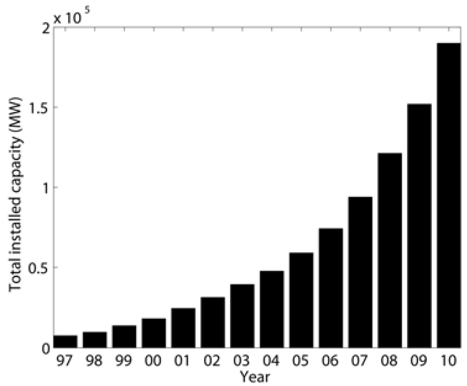
:1. Introduction


2. Methodology
2.1. The Prognostic Mesoscale Model, MM5
2.2. The CALMET Diagnostic Meteorological Model
2.3. Model validation
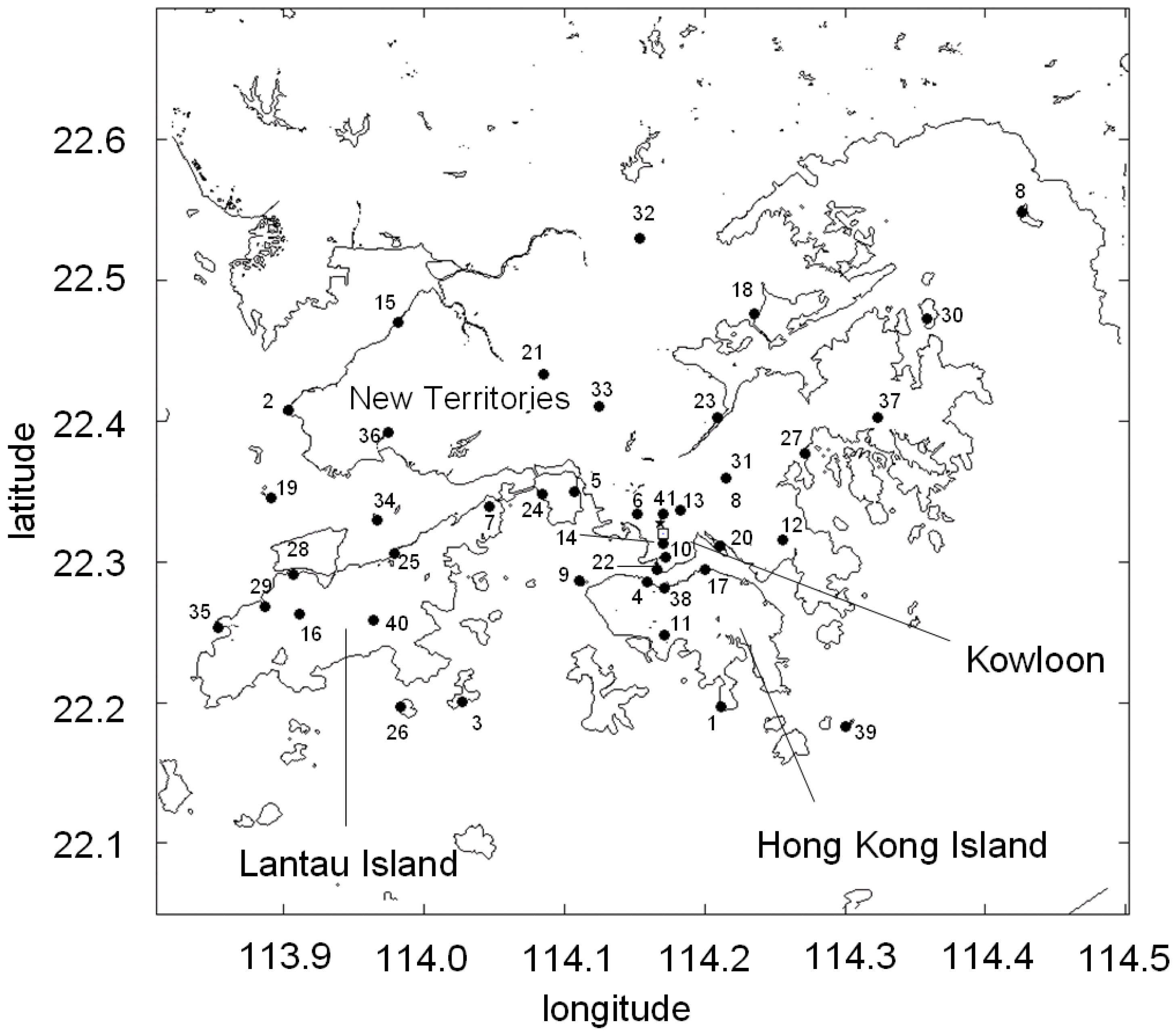
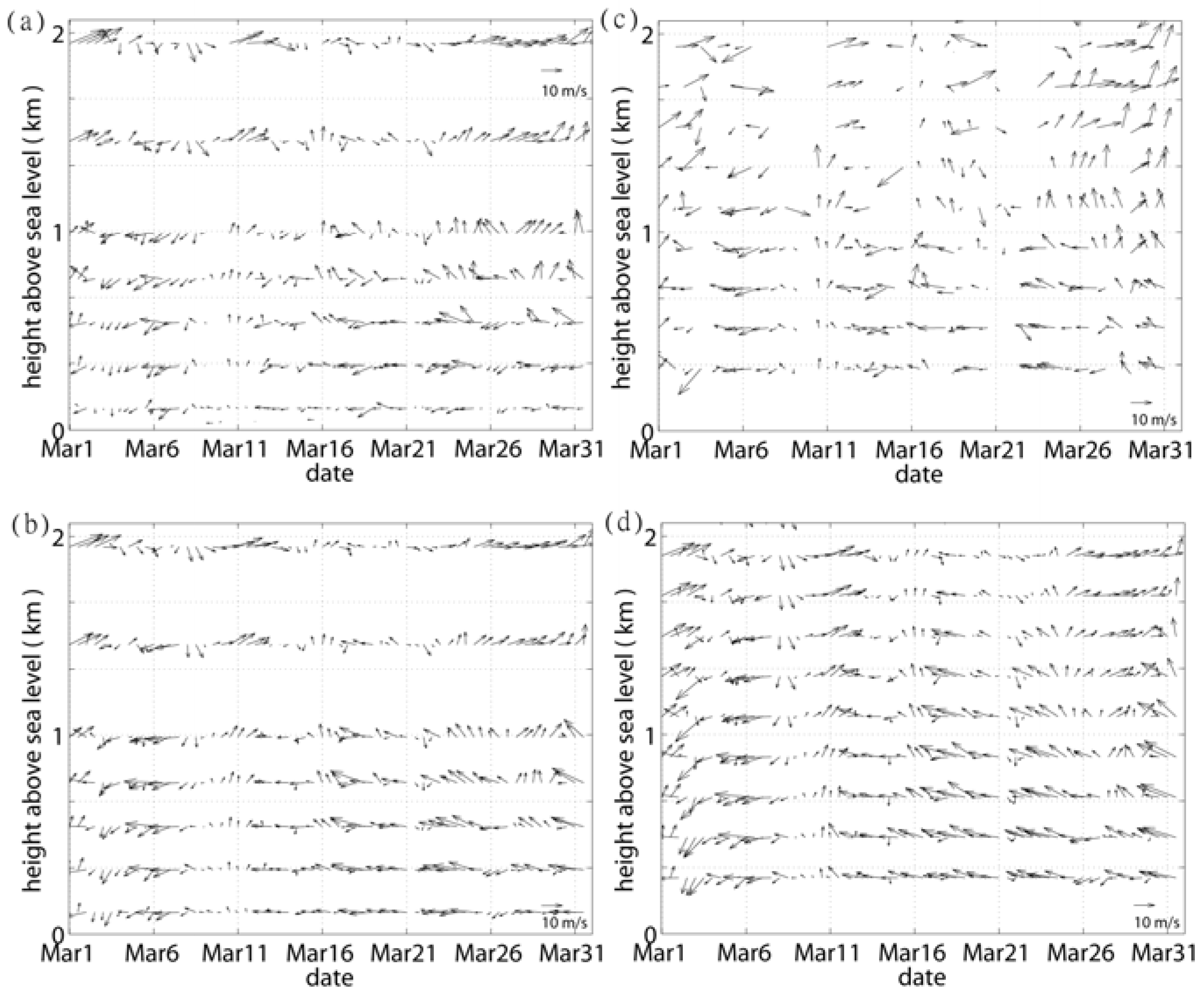
2.3.1. Comparison of Surface Stations and Upper Sounding Data


| Station name | Observed Mean Speed (m/s) | Model Mean Speed (m/s) | Observed SD | Model Result SD | RMSE | I | % of valid data | |
|---|---|---|---|---|---|---|---|---|
| 1 | Bluff Head (BHD) | 3.67 | 3.53 | 1.98 | 1.72 | 0.41 | 0.99 | 95.3 |
| 2 | Black Point (BPT) | 3.06 | 2.92 | 2.42 | 2.04 | 0.52 | 0.99 | 93.6 |
| 3 | Cheung Chau (CCH) | 5.00 | 4.79 | 2.51 | 2.53 | 0.27 | 0.99 | 90.8 |
| 4 | Central: Star Ferry Pier (CEN) | 2.97 | 3.03 | 1.74 | 1.72 | 0.35 | 0.99 | 99.6 |
| 5 | Ching Pak House, Tsing Yi (CPH) | 3.76 | 3.26 | 1.60 | 1.47 | 0.39 | 0.98 | 99.5 |
| 6 | Cheung Sha Wan (CSW) | 2.49 | 2.63 | 1.15 | 1.21 | 0.45 | 0.96 | 99.6 |
| 7 | East Lantau (ELN) | 3.93 | 3.81 | 2.21 | 2.12 | 0.18 | 0.99 | 99.2 |
| 8 | Ping Chau (EPC) | 1.44 | 2.77 | 0.84 | 1.98 | 0.18 | 0.99 | 88.9 |
| 9 | Green Island (GI) | 6.15 | 5.83 | 3.35 | 3.23 | 0.18 | 0.99 | 96.5 |
| 10 | Hong Kong Observatory (HKO) | 2.93 | 3.35 | 1.69 | 1.91 | 0.77 | 0.95 | 99.0 |
| 11 | Wong Chuk Hang (HKS) | 2.85 | 2.67 | 1.55 | 1.44 | 0.18 | 0.99 | 99.6 |
| 12 | Tseung Kwan O (JKB) | 1.85 | 1.93 | 0.98 | 1.19 | 0.22 | 0.99 | 99.7 |
| 13 | Kowloon Tsai (KLT) | 2.46 | 2.56 | 1.13 | 1.45 | 0.86 | 0.88 | 99.1 |
| 14 | King’s Park (KP) | 3.09 | 3.73 | 1.32 | 2.21 | 1.76 | 0.76 | 79.2 |
| 15 | Lau Fau Shan (LFS) | 3.21 | 3.21 | 1.58 | 1.59 | 0.09 | 0.99 | 99.8 |
| 16 | Nei Lak Shan (NLS) | 7.14 | 6.93 | 4.03 | 3.64 | 0.79 | 0.99 | 97.7 |
| 17 | North Point (NP) | 4.09 | 3.40 | 1.80 | 1.53 | 0.76 | 0.94 | 99.9 |
| 18 | Tai Mei Tuk (PLC) | 4.05 | 3.98 | 2.07 | 2.11 | 0.21 | 0.99 | 97.6 |
| 19 | Sha Chau (SC) | 5.62 | 5.45 | 2.67 | 2.74 | 0.10 | 0.99 | 98.4 |
| 20 | Kai Tak (SE) | 3.65 | 3.01 | 1.50 | 1.33 | 0.68 | 0.94 | 94.0 |
| 21 | Shek Kong (SEK) | 3.19 | 2.73 | 1.64 | 1.40 | 0.38 | 0.98 | 98.9 |
| 22 | Star Ferry: Tsim Sha Tsui (SF) | 3.55 | 3.74 | 2.06 | 2.25 | 0.50 | 0.99 | 99.6 |
| 23 | Sha Tin (SHA) | 2.53 | 2.34 | 1.07 | 1.07 | 0.45 | 0.95 | 99.5 |
| 24 | Shell Tsing Yi Installation (SHL) | 2.52 | 2.44 | 1.59 | 1.50 | 0.16 | 0.99 | 99.3 |
| 25 | Siu Ho Wan (SHW) | 3.82 | 3.62 | 2.15 | 1.87 | 0.80 | 0.96 | 80.3 |
| 26 | Shek Kwu Chau (SKC) | 5.37 | 4.61 | 2.81 | 2.26 | 0.98 | 0.96 | 69.8 |
| 27 | Sai Kung (SKG) | 2.97 | 2.70 | 1.93 | 1.66 | 0.46 | 0.98 | 99.8 |
| 28 | Sha Lo Wan (SLW) | 3.61 | 3.57 | 2.32 | 2.28 | 0.23 | 0.99 | 98.6 |
| 29 | Sham Wat (SW) | 2.55 | 2.79 | 1.36 | 1.68 | 0.24 | 0.99 | 98.9 |
| 30 | Tap Mun (TAP) | 3.20 | 3.18 | 1.74 | 1.79 | 0.15 | 0.99 | 99.7 |
| 31 | Tate’s Cairn (TC) | 6.57 | 4.97 | 3.21 | 2.19 | 1.93 | 0.88 | 98.0 |
| 32 | Ta Kwu Ling (TKL) | 2.59 | 2.49 | 1.38 | 1.38 | 0.07 | 0.99 | 99.8 |
| 33 | Tai Mo Shan (TMS) | 5.80 | 5.99 | 3.10 | 3.05 | 0.62 | 0.99 | 99.6 |
| 34 | Tai Mo To (TMT) | 4.80 | 4.66 | 2.31 | 2.25 | 0.17 | 0.99 | 97.6 |
| 35 | Tai O (TO) | 4.46 | 4.00 | 3.54 | 3.16 | 0.23 | 0.99 | 97.4 |
| 36 | Tuen Mun (TUN) | 2.60 | 2.51 | 1.38 | 1.20 | 0.28 | 0.99 | 89.0 |
| 37 | Tsak Yue Wu (TYW) | 1.78 | 1.89 | 1.66 | 1.56 | 0.14 | 0.99 | 98.7 |
| 38 | Wan Chai (WCN) | 4.65 | 4.55 | 2.36 | 2.49 | 0.29 | 0.99 | 99.7 |
| 39 | Waglan Island (WGL) | 6.82 | 6.17 | 3.12 | 3.25 | 0.08 | 0.99 | 97.3 |
| 40 | Yi Tung Shan (YTS) | 7.16 | 6.96 | 3.63 | 3.45 | 0.68 | 0.99 | 98.4 |
| 41 | Yau Yat Chuen (YYC) | 2.81 | 3.08 | 1.90 | 1.93 | 0.85 | 0.95 | 98.7 |
| Station name | Observed Mean Speed (m/s) | Model Mean Speed (m/s) | Observed SD | Model Result SD | RMSE | I | % of valid data | |
|---|---|---|---|---|---|---|---|---|
| 1 | Tuen Mun (TUN) | 2.60 | 2.86 | 1.38 | 1.53 | 1.15 | 0.84 | 89.0 |
| 2 | Cheung Sha Wan (CSW) | 2.41 | 3.06 | 1.17 | 1.77 | 1.38 | 0.77 | 99.6 |
| 3 | Cheung Chau (CCH) | 5.02 | 4.32 | 2.51 | 2.47 | 1.30 | 0.93 | 90.8 |

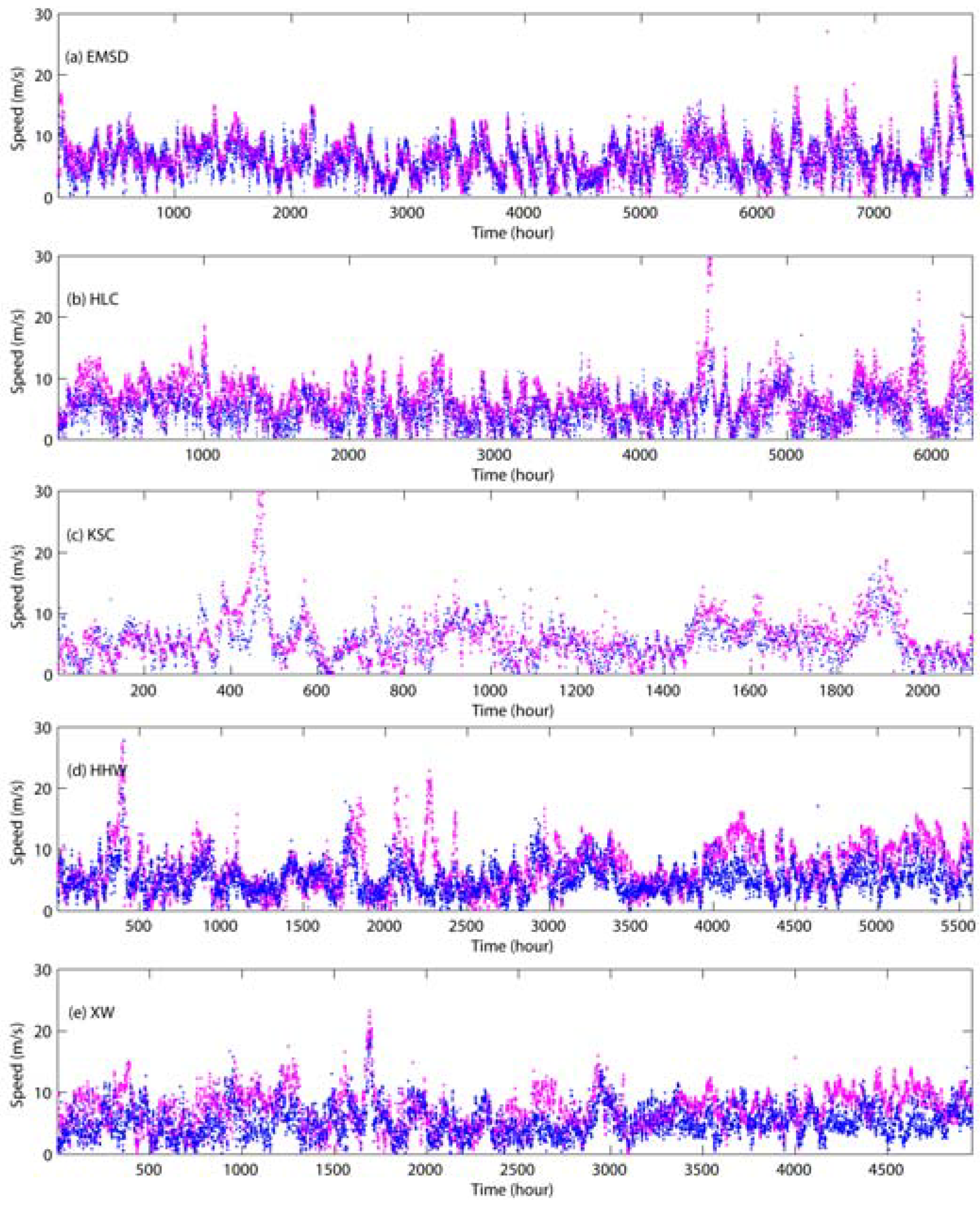
2.3.2. Comparison of Field Data
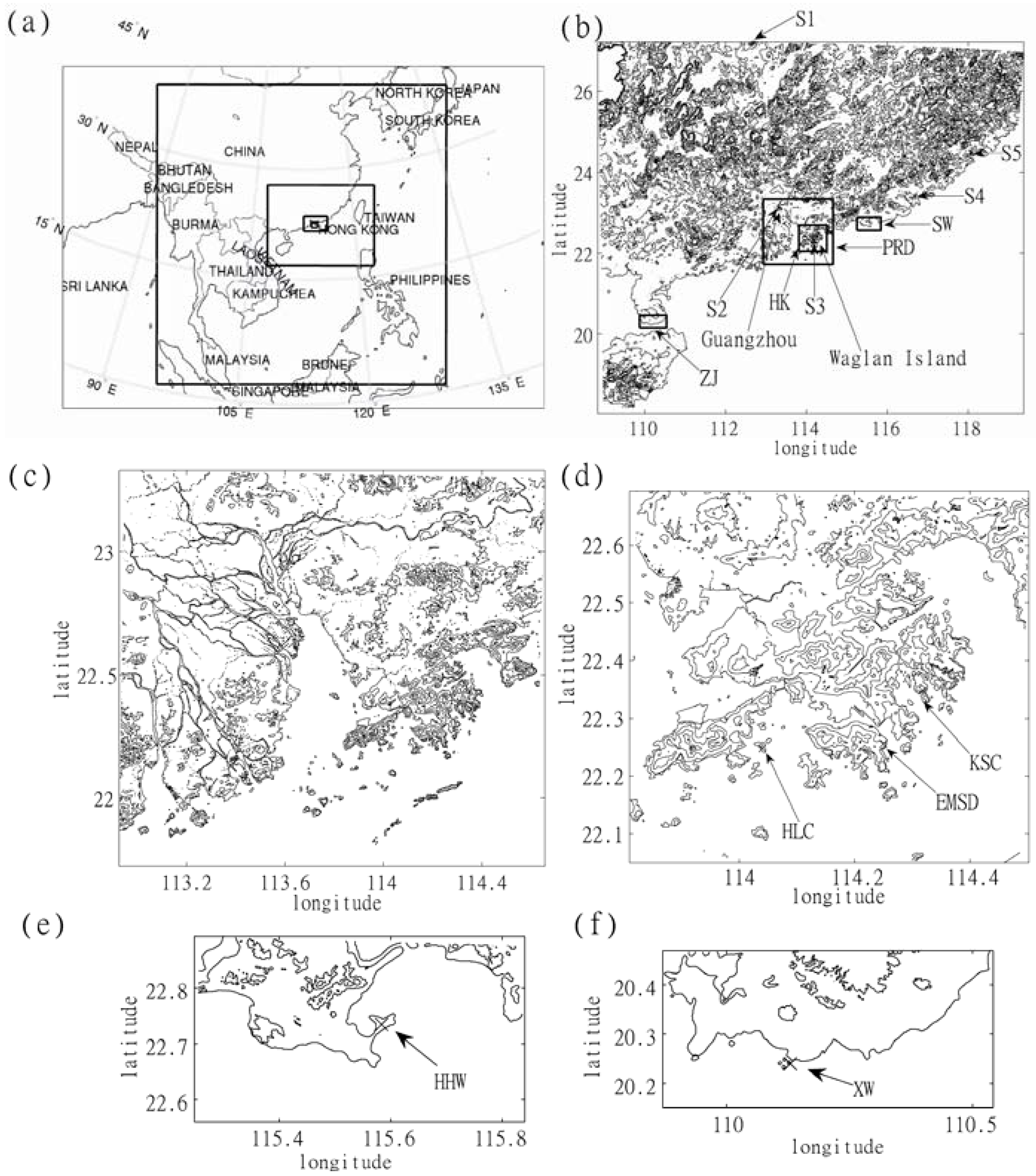
- (1)
- One station from the Electrical and Mechanical Services Department (EMSD) in HK
- (2)
- Two stations from China Light Power (CLP) in HK
- (3)
- One station in Hung Hai Wan (HHW) in Shan Wei(SW) (China)
- (4)
- One station in Xu Wen (XW) in Zhan Jiang(ZJ) (China)

| Station name | Observed Mean Speed (m/s) | Model Mean Speed (m/s) | Observed SD | Model Result SD | RMSE | I | % of valid data | |
|---|---|---|---|---|---|---|---|---|
| 1 | EMSD | 5.95 | 6.53 | 2.91 | 3.02 | 1.32 | 0.75 | 88.2 |
| 2 | Hei Ling Chau (HLC) | 4.80 | 5.46 | 2.71 | 2.41 | 1.36 | 0.70 | 97.0 |
| 3 | Kau Sai Chau (KSC) | 5.40 | 5.90 | 3.08 | 3.78 | 1.12 | 0.75 | 96.8 |
| 4 | Hung Hai Wan (HHW) | 5.25 | 6.10 | 2.57 | 3.75 | 1.47 | 0.60 | 95.5 |
| 5 | Xu Wen (XW) | 5.28 | 6.00 | 2.54 | 3.02 | 1.54 | 0.63 | 86.9 |
3. Results and Discussions
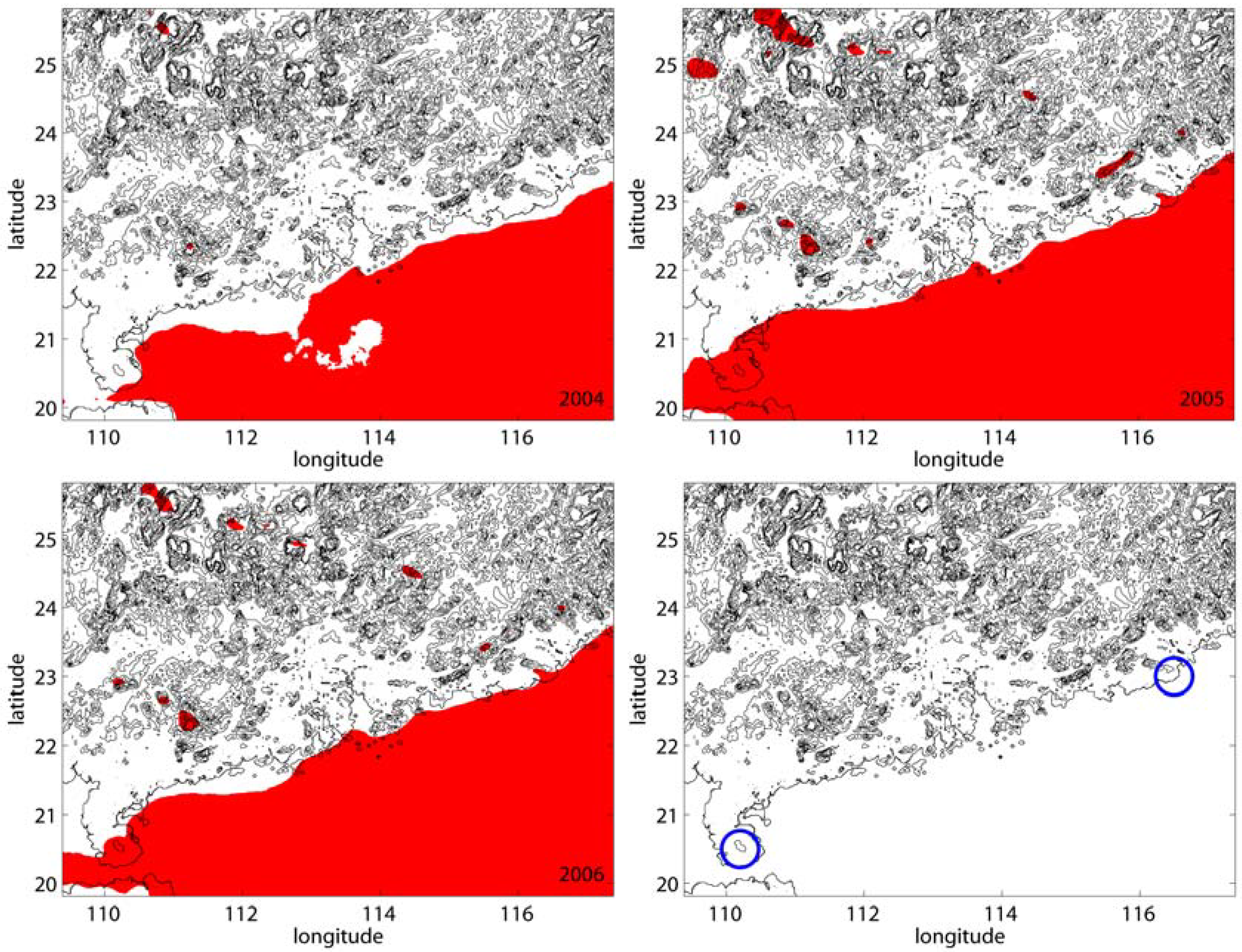
3.1 Wind Availability over Study Area


3.2. Weibull Function, Wind Map and Wind Power


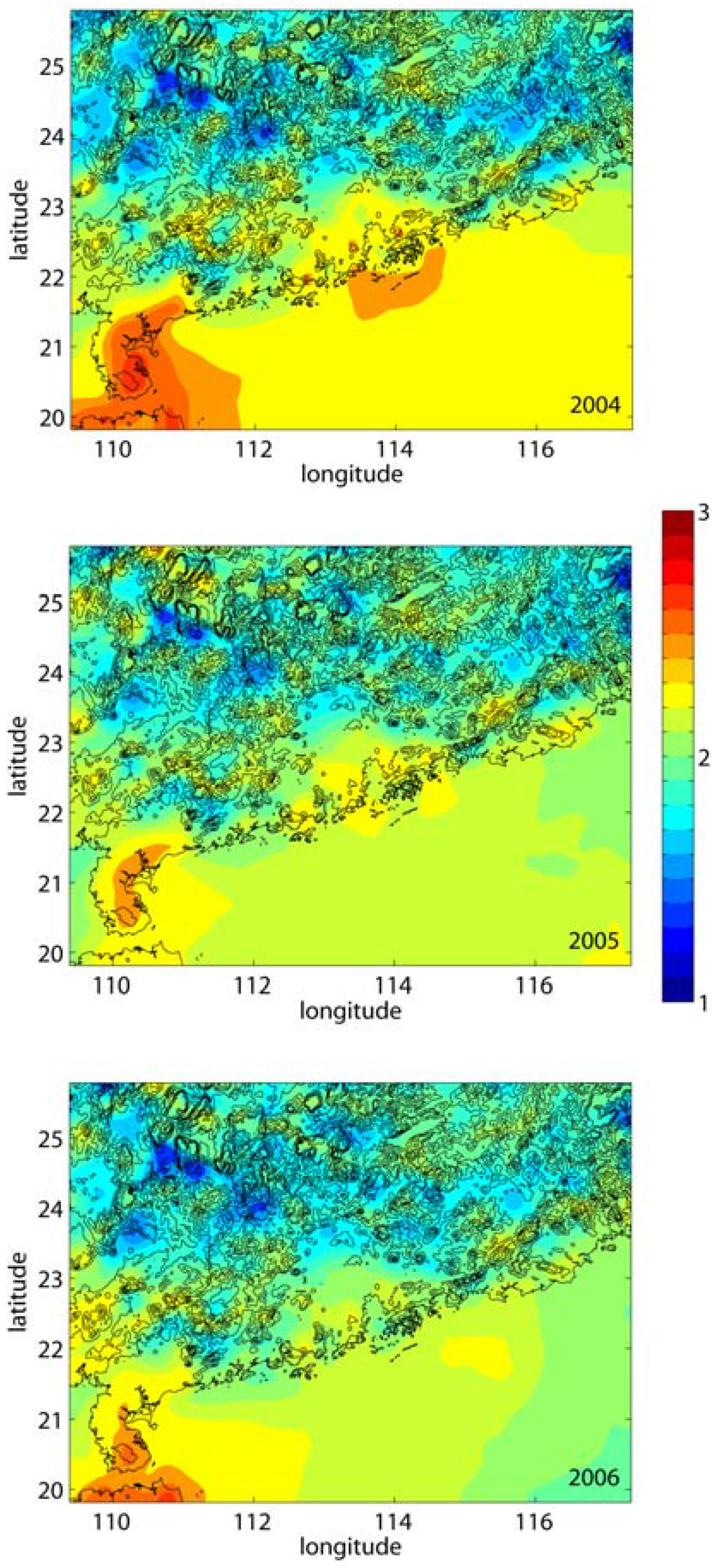
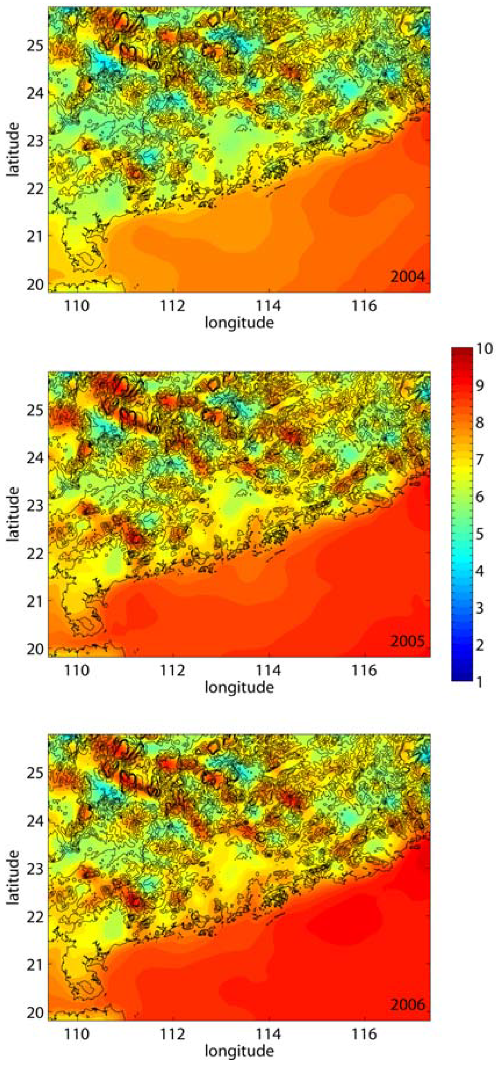
3.2.1. The Weibull Density Function in Guangdong Province


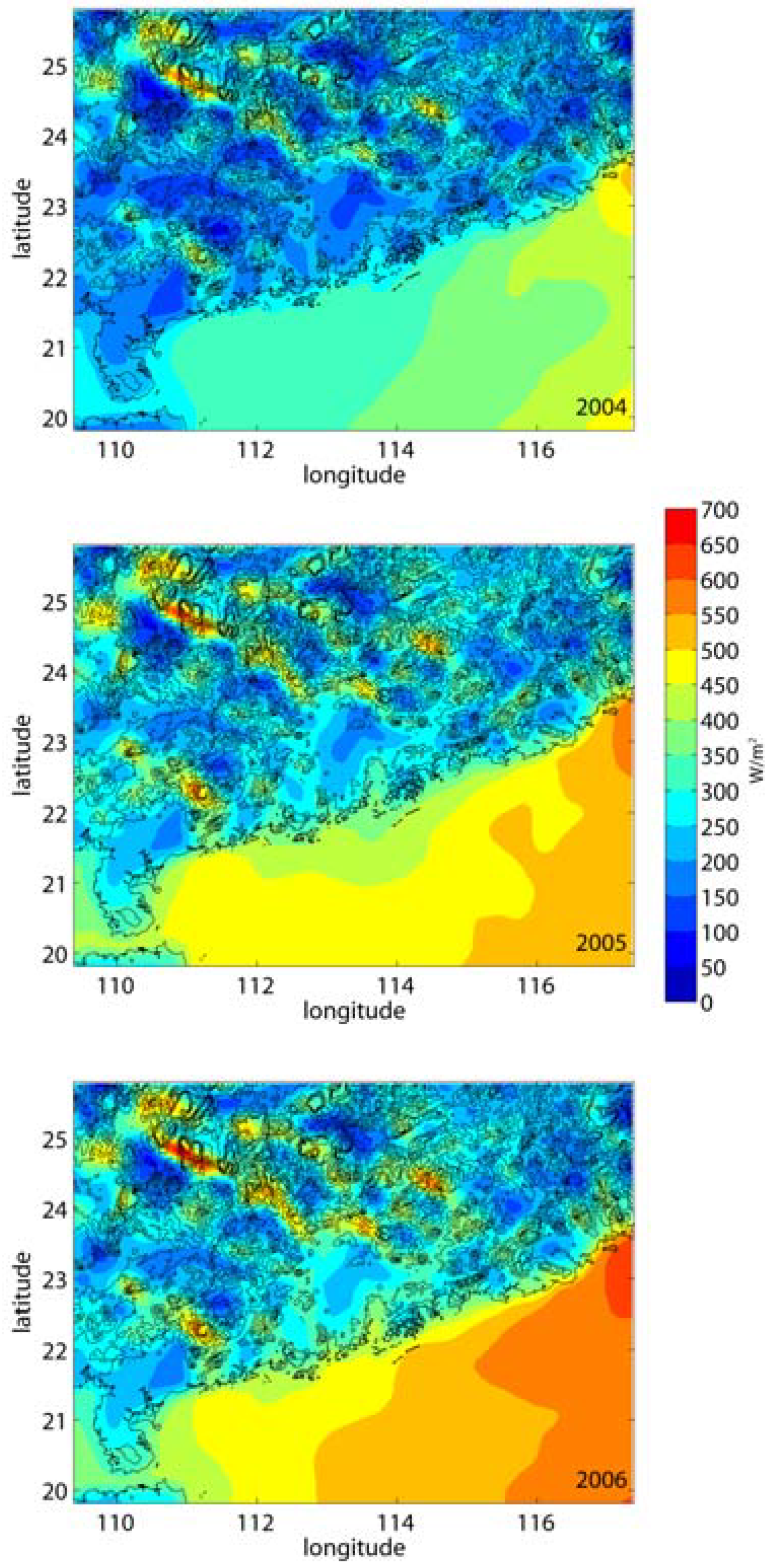
3.2.2. Annual Average Wind Power


4. Conclusions
Acknowledgements
References and Notes
- WWEA. WWEA Sustainability and Due Diligence Guidelines; World Wind Energy Association, 2005. Available online: http://www.wwindea.org/home/images/stories/pdfs/wwea_05_11-10.pdf.
- WWEA. World Wind Energy Report 2008; World Wind Energy Association, 2008; Available online: http://www.wwindea.org/home/index.php.
- GWEC. Global Wind 2008 Report; Global Wind Energy Council, 2008. Available online: http://www.gwec.net/.
- Fung, W.S. A feasibility study and engineering design of wind power in Hong Kong. Master Thesis, The Hong Kong Polytechnic University, Hong Kong, China, 1999. [Google Scholar]
- Li, G. Feasibility of large-scale offshore wind power for Hong Kong - a preliminary study. J. Renew. Energy 2000, 21, 387–402. [Google Scholar] [CrossRef]
- Lu, L.; Yang, H.X. Investigation on wind power potential on Hong Kong islands - an analysis of wind power and wind turbine characteristics. J. Renew. Energy 2002, 27, 1–12. [Google Scholar] [CrossRef]
- Zhou, W.; Yang, H.X.; Fang, Z.H. Wind power potential and characteristic analysis of the Pearl River Delta region, China. J. Renew. Energy 2006, 31, 739–753. [Google Scholar] [CrossRef]
- Dudhia, J. A nonhydrostatic version of the Penn State-NCAR Mesoscale Model: Validation tests and simulation of an Atlantic cyclone and cold front. Mon. Wea. Rev. 1993, 121, 1493–1513. [Google Scholar] [CrossRef]
- Grell, G.A.; Dudhia, J.; Stauffer, D.R. A description of the fifth generation Penn State-NCAR Mesoscale Model (MM5). NCAR Tech. Note NCAR/TN-398 +STR 1994, 138–139. [Google Scholar]
- Wang, X.M.; Lin, W.S.; YanG, L.M.; Deng, R.R.; Lin, H. A numerical study of influences of urban land-use change on ozone distribution over the Pearl River Delta region, China. Tellus B 2007, 59, 633. [Google Scholar] [CrossRef]
- Lin, C.Y.; Wang, Z.F.; Chou, C.C.K.; Chang, C.C.; Liu, S.C. A numerical study of an autumn high ozone episode over southwestern Taiwan. J. Atmos. Environ. 2007, 41, 3684–3701. [Google Scholar] [CrossRef]
- Wei, X.L.; Li, Y.S.; Lam, K.S.; Wang, A.Y.; Wang, T.J. Impact of biogenic VOC emissions on a tropical cyclone-related ozone episode in the Pearl River Delta region, China. J. Atmos. Environ. 2007, 41, 7851–7864. [Google Scholar]
- Chune, S.; Fernando, H.J.S.; Wang, Z.F.; An, X.Q.; Wu, Q.Z. Tropospheric NO2 columns over East Central China: Comparisons between SCIAMACHY measurements and nested CMAQ simulations. J. Atmos. Environ. 2008, 42, 7165–7173. [Google Scholar]
- Huang, J.P.; Fung, J.C.H.; Lau, A.K.H.; Qin, Y. Numerical simulation and process analysis of typhoon-related ozone episodes in Hong Kong. J. Geophys. Res. 2005, 110, D05301. [Google Scholar] [CrossRef]
- Huang, J.P.; Fung, J.C.H.; Lau, A.K.H. Integrated processes analysis and systematic meteorological classification of ozone episodes in Hong Kong. J. Geophys. Res. 2006, 111, D20309. [Google Scholar] [CrossRef]
- Hong, S.Y.; Pan, H.L. Nonlocal boundary layer vertical diffusion in a medium-range forecast model. Mon. Weather Rev. 1996, 124, 2322–2339. [Google Scholar] [CrossRef]
- Ding, A.; Wang, T.; Zhao, M.; Wang, T.; Li, Z. Simulation of sea-land breezes and a discussion of their implications on the transport of air pollution during a multi-day ozone episode in the Pearl River Delta of China. J. Atmos. Environ. 2004, 38, 6737–6750. [Google Scholar] [CrossRef]
- Seaman, N.L.; Stauffer, D.R.; Lario-Gibbs, A.M. A Multiscale Four- Dimensional Data Assimilation System Applied in the San Joaquin Valley during SARMAP. Part I: Modeling Design and Basic Performance Characteristics. J. Appl. Meteorol. 1995, 34, 1739–1761. [Google Scholar] [CrossRef]
- Fung, J.C.H.; Lau, A.K.H.; Lam, J.S.L.; Yuan, Z. Observational and modeling analysis of a severe air pollution episode in western Hong Kong. J. Geophys. Res. 2005, 110, D09105. [Google Scholar]
- Douglas, S.G.; Kessler, R.C. User’s guide to the diagnostic wind model (Version 1.0); Systems Applications Inc.: San Rafel, CA, USA, 1988. [Google Scholar]
- Chandrasekar, A.; Philbrick, R.; Clark, B.; Doddridge, B.; Georgopoulos, P. Evaluating the performance of a computationally efficient MM5/CALMET system for developing wind field inputs to air quality models. J. Atmos. Environ. 2003, 37, 3267–3276. [Google Scholar] [CrossRef]
- Chuang, M.T.; Fu, J.S.; Jang, C.J.; Chan, C.C.; Ni, P.C.; Lee, C.T. Simulation of long-range transport aerosols from the Asian Continent to Taiwan by a Southward Asian high-pressure system. Sci. Total Environ. 2008, 406, 168–179. [Google Scholar]
- Streets, D.G.; Fu, J.S.; Jang, C.J.; Hao, J.M.; He, K.B.; Tang, X.Y.; Zhang, Y.H.; Wang, Z.F.; Li, Z.P.; Zhang, Q.; Wang, L.T.; Wang, B.Y.; Yu, c. Air quality during the 2008 Beijing Olympic Games. J. Atmos. Environ. 2007, 41, 480–492. [Google Scholar] [CrossRef]
- Jackson, B.; Chau, D.; Gurer, K.; Kaduwela, A. Comparison of ozone simulations using MM5 and CALMET/MM5 hybrid meteorological fields for the July/August 2000 CCOS episode. J. Atmos. Environ. 2006, 40, 2812–2822. [Google Scholar] [CrossRef]
- Yim, S.H.L.; Fung, J.C.H.; Lau, A.K.H.; Kot, S.C. Developing a high-resolution wind map for a complex terrain with a coupled MM5/CALMET system. J. Geophys. Res. 2007, 112, D05106. [Google Scholar] [CrossRef]
- Truhetz, H.; Gobiet, A.; Kirchengast, G. Evaluation of a dynamic-diagnostic modeling approach to generate highly resolved wind climatologies in the Alpine region. Meteorol. Z. 2007, 16, 191–201. [Google Scholar] [CrossRef]
- Barna, M.B.; Lamb, B.K.; O’Neill, S.M.; Westberg, H.; Figueroa-Kaminsky, C.; Otterson, S.; Bowman, C.; DeMay, J. Modeling ozone formation and transport in the Cascadia region of the Pacific Northwest. J. Appl. Meteorol. 2000, 39, 349–366. [Google Scholar] [CrossRef]
- Lu, R.; Turco, R.P.; Jacobson, M.A. An integrated air pollution modeling system for urban and regional scales: 1. Simulations for SCAQS 1987. J. Geophys. Res. 1997, 102, 6063–6079. [Google Scholar] [CrossRef]
- Barna, M.B.; Lamb, B.K. Improving ozone modeling in regions of complex terrain using observational nudging in a prognostic meteorological model. J. Atmos. Environ 2000, 34, 4889–4906. [Google Scholar] [CrossRef]
- Weisser, D. A wind energy analysis of Grenada: An estimation using the 'Weibull' density function. J. Renew. Energy 2003, 28, 1803–1812. [Google Scholar] [CrossRef]
- Mukund, R.P. Wind and Solar Power Systems, 2nd ed.; CRC Press: Boca Raton, FL, USA, 2006. [Google Scholar]
- Dupont, S.; Otte, T.; Ching, J. Simulation of meteorological fields within and above urban and rural canopies with a mesoscale model (MM5). Boundary Layer Meteorol. 2004, 113, 111–158. [Google Scholar] [CrossRef]
- Abderrazzaq, M.H. Energy production assessment of small wind farms. J. Renew. Energy 2004, 29, 2261–2272. [Google Scholar] [CrossRef]
- Walker, J.F.; Jenkins, N. Wind energy technology; John Wiley & Sons Inc: New York, NY, USA, 1997. [Google Scholar]
- Ferguson, A.R.B. Wind Power: Benefits and Limitations. In Biofuels, Solar and Wind as Renewable Energy Systems; Springer: Dordrecht, the Netherlands, 2008; pp. 133–151. [Google Scholar]
- Tyner, G., Sr. Net Energy from Wind Power; Minnesotans for Sustainability, 2002. [Google Scholar]
© 2009 by the authors; licensee Molecular Diversity Preservation International, Basel, Switzerland. This article is an open-access article distributed under the terms and conditions of the Creative Commons Attribution license (http://creativecommons.org/licenses/by/3.0/).
Share and Cite
Yim, S.H.L.; Fung, J.C.H.; Lau, A.K.H. Mesoscale Simulation of Year-to-Year Variation of Wind Power Potential over Southern China. Energies 2009, 2, 340-361. https://doi.org/10.3390/en20200340
Yim SHL, Fung JCH, Lau AKH. Mesoscale Simulation of Year-to-Year Variation of Wind Power Potential over Southern China. Energies. 2009; 2(2):340-361. https://doi.org/10.3390/en20200340
Chicago/Turabian StyleYim, Steve H.L., Jimmy C.H. Fung, and Alexis K.H. Lau. 2009. "Mesoscale Simulation of Year-to-Year Variation of Wind Power Potential over Southern China" Energies 2, no. 2: 340-361. https://doi.org/10.3390/en20200340