Classification and Clustering of Electricity Demand Patterns in Industrial Parks

Abstract

Understanding of energy consumption patterns is extremely important for optimization of resources and application of green trends. Traditionally, analyses were performed for large environments like regions and nations. However, with the advent of Smart Grids, the study of the behavior of smaller environments has become a necessity to allow a deeper micromanagement of the energy grid. This paper presents a data processing system to analyze energy consumption patterns in industrial parks, based on the cascade application of a Self-Organizing Map (SOM) and the clustering k-means algorithm. The system is validated with real load data from an industrial park in Spain. The validation results show that the system adequately finds different behavior patterns which are meaningful, and is capable of doing so without supervision, and without any prior knowledge about the data.

1. Introduction

Electricity is an indispensable resource for global and national economies. In order to optimize its usage, both for environmental reasons and to keep prices competitive, utilities are constantly trying to adjust energy production to the actual demand. Typically, this adaptation has been performed at high, aggregated levels (nation or region-wide), but recently, the development of Smart Grids has opened the door for disaggregated control and optimization of energy production in smaller environments, such as cities or industrial parks. These localized environments can normally be considered microgrids (groups of energy producers and consumers, connected together, which can operate with a certain degree of independence) [1], which present advantages such as precise monitoring of low-level network elements (even homes, thanks to Smart Meters) and precise control of small generation and storage elements (such as small wind turbines or solar panels); hence a more precise matching of generation and demand is possible in real time, and transportation losses are reduced because generators are near consumers.

However, while global demand was relatively easy to predict and understand thanks to the aggregation of large numbers of elements across regions, forecast in disaggregated microgrids is much more difficult, because the relative contribution of each element’s behaviour to the aggregate picture is much more important and consequently, variations are much larger.

As mentioned, industrial parks, which can be considered microgrids from the energy network point of view, are very important actors in the energy market of a country. It is necessary that aggregators control and manage these spaces, trying at the same time to optimize their energy consumption and the energy rewards offered. Several tools are available to perform this optimization, such as Demand Response (DR), which means accommodating some of the demand (by means of reward reductions or direct control of smart loads with relaxed time restrictions) to the most suitable time schedule of the generators (for instance shifting demand from consumption peaks to valleys to obtain a flatter curve with a lower maximum power peak, or to accommodate some operations during periods of high wind to size wind turbines).

The importance of power management in industrial parks has been widely demonstrated in the literature, as for instance in [2,3,4,5,6]. Park [7] presents the simulation of the operation in an industrial plant with distributed metering. Zareipoor et al. [8] present a scenario of industrial plant operation based on prices, for which the management and control of the industrial parks is essential. Laboratory modeling, monitoring and control of a microgrid, extrapolated to industrial parks, is shown in [9].

DR and other optimization methods are not possible without a detailed knowledge of the behavior of the industrial park. In an industrial park different types of industries with very different electricity consumption habits normally coexist, so traditional forecasting and data analysis methods, suitable only for aggregated demand in big regions, are no longer applicable. This work presents a data analysis method for clustering daily load curves in industrial park environments, classifying days in different groups with recognizable load patterns and meaningful characteristics. This method is based on pattern recognition through a Self-Organizing Map (SOM) for classification of load curves, and then forming clusters via a k-means algorithm.

A SOM is a specific Artificial Neural Network (ANN) architecture designed to cluster data that has been used in the past for different purposes related with energy data analysis, such as classification of aggregated consumption data [10] at a regional scale, or to perform Short Term Load Forecasting (STLF) [11]. Marín et al. [12] applied SOM for load curve classification of a large area of central Spain; Mori and Itagaki [13] show a reconstruction of the groups obtained by Radial Basis Function Network (RBFN), after using SOM for data classification. SOMs have also been used to forecast electricity demand in Brazil [14], and China [15]. However, all this works deal with aggregated demand in big environments (such as regions and nations) and are not directly applicable to microgrid-size scenarios such as industrial parks.

Therefore, the aim of this paper is to present a data analysis system to cluster load curves in industrial parks based on SOM ANN, and validate it using real world data. Some initiatives roughly based on the same approach have been already reported in the literature, but with different purposes. For instance, [16,17] present load pattern analysis tools to cluster different types of clients. The main difference with the work presented here is that, while those studies were made to discriminate and group load curves generated by different entities, this work deals with discriminating different consumption patterns of a single entity which appear under different conditions in time.

After this introduction, the architecture of the system is presented in Section 2. Section 3 and Section 4 present the real world case study for validation and the results of the application of the system, respectively. Finally, Section 5 summarizes the conclusions of this work.

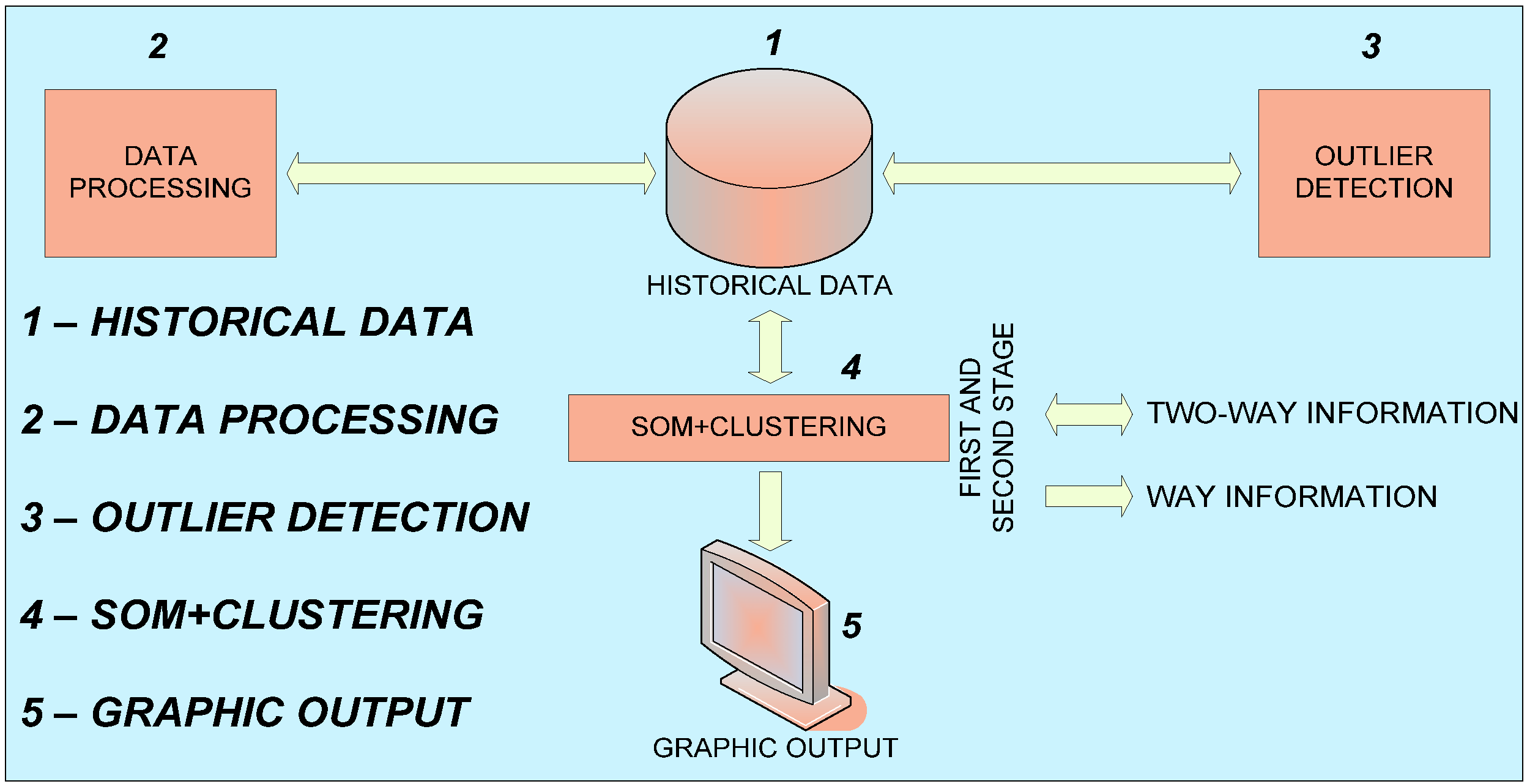
2. System Architecture

As mentioned in the introduction, the objective of the system presented along this work is to cluster the daily load curves of an industrial park in different meaningful groups. This will allow the classification of days in different groups, each of them presenting a distinct load curve pattern and a set of meaningful features. The system is comprised by a SOM to classify the load curves, followed by a clustering with the k-means algorithm. The architecture of the System is depicted in Figure 1. It comprises the following modules:

• Historical Data: the database storing the consumption data by quarter-hours, including calendar information for each sample such as day, month, year, workability and day of the week.
• Data Pre-Processing: to clean the database (removing erroneous samples or interpolating, when possible, missing data) and accommodate the format to the input of the following examples (e.g., aggregating quarter-hour samples in hourly values).
• Outlier Detection: An implementation of the Principal Component Analysis (PCA) method to identify and remove erroneous data (produced for instance due to monitoring hardware malfunctions), discriminating them from proper data which shows abnormal values (such as a bank holiday, which normally presents an abnormal load curve).
• SOM + CLUSTERING: represents the combined application of SOM and k-means.
• Graphic Output: its main task is to send the information of the results given by the previous stage, to be displayed graphically.

Figure 1. System Architecture.

Figure 1. System Architecture.

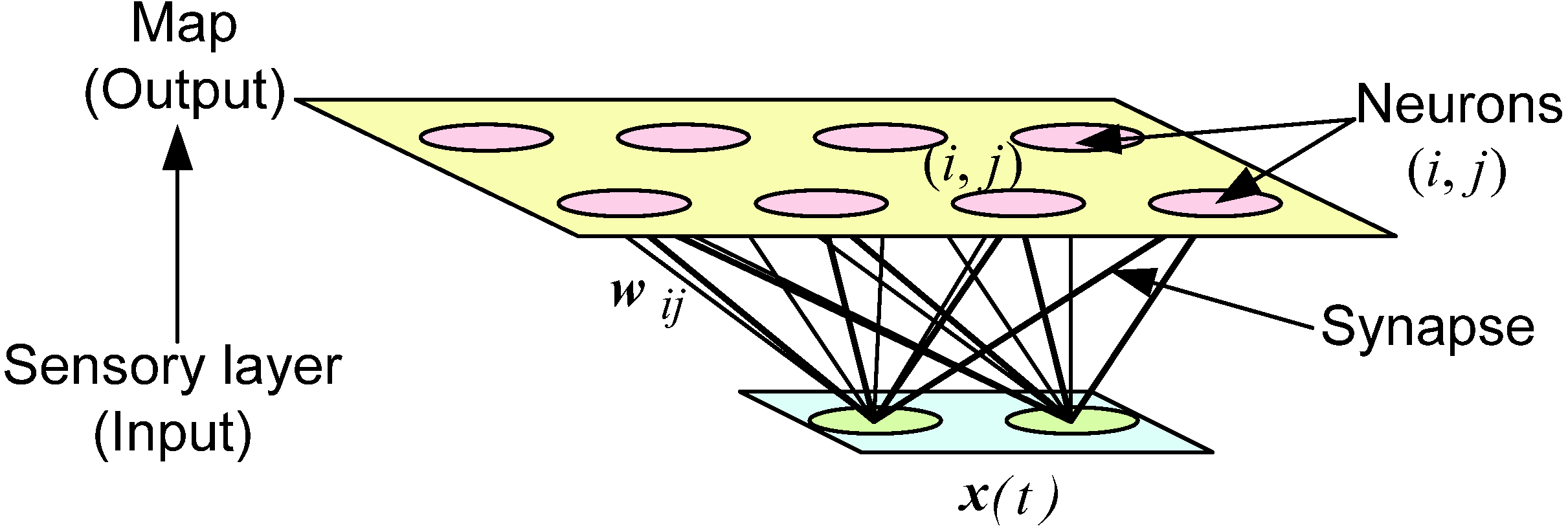
2.1. Self-Organizing Map

First described by Kohonen, SOMs are an ANN architecture designed for unsupervised classification of data into clusters [18,19,20]. The neurons are arranged in two-layer architecture. The first is the sensory or input layer, consisting of m neurons (as many neurons as input variables), whose role is to distribute information from the input space to the second layer. The second layer forms a map of features conforming a grid of nx × ny neurons operating in parallel. Input neurons are label with the index k (1 ≤ k ≤ m), and nx × ny neurons in the map with a pair of indices I ≡ (i,j) (1 ≤ I ≤ nx, 1 ≤ j ≤ ny), which determines its spatial location. Each input neuron (k) is connected to all neurons (i,j) on the map by a synaptic weight w_ij. The representation of this architecture is shown in Figure 2.

Figure 2. SOM architecture.

Figure 2. SOM architecture.

The SOM presents a competitive learning approach: when the input vector [x(t)] is presented to the network, the similarity between this vector and each neuron’s synaptic weight (w_ij) is computed. The neuron whose weight vector is most similar to the input is considered the winner. Then, the synaptic weight of the is modified to be closer to x(t), so when confronted with similar inputs in the future, the neuron will response will be even stronger. This process is repeated for all input vectors so that the different reference vectors harmonize with specific domains of the input variables, known as Voronoi domains [21].

2.2. Clustering

Clustering means partitioning a data set into a set of C clusters Q_i, I = 1,…,C; the word normally implies that this partitioning is unsupervised, i.e., done without any prior knowledge about the data structure, such as number of groups, their definition, or any sample members of the clusters. A widely adopted definition of optimal clustering is a partitioning that minimizes distances within and maximizes distances between clusters.

The k-means algorithm (detailed at [22]) is one of the simplest and most widely used unsupervised learning algorithms that solves the clustering problem. The procedure follows a simple and easy way to classify a given data set through a certain number of clusters fixed a priori. The main idea is to define k centroids, one for each cluster. Next step is to take each point belonging to a given data set and associate it to the nearest centroid. When no point is pending, the first step is completed and an early grouping is done. At this point, it is necessary to re-calculate k new centroids as barycentres of the clusters resulting from the previous step. After having these k new centroids, a new iteration of the assignation of data set points to the nearest new centroid has to be performed. The k centroids change their location step by step until they no longer move meaningfully.

2.3. Combination of Algorithms

Vesanto et al. [23] show that clustering of the SOM renders better results than clustering the data directly. The primary benefit of the two-level approach (SOM + Clustering) is the reduction of the computational cost: even with a relatively small number of samples, many clustering algorithms (especially hierarchical ones) become excessively resource intensive. For this reason, it is convenient to cluster a set of prototypes rather than proceed directly with the raw data. Another benefit is noise reduction: after SOM, the prototypes are local averages of the data and, therefore, less sensitive to random variations than the original data.

3. Case of Study

3.1. Research Data and Test Scenario

In order to validate the previously described approach, a dataset provided by Iberdrola, a Spanish utility was used. This dataset includes information from 1 January 2008 to 31 December 2010, from the “Las Casas” industrial park located in Soria (Castilla y León, Spain). The data fields provided are: day number, day of the week, month, year, workability and the load curves (24 values) for each day. The range of consumption varies from 0.3 to 7 MW, definitely much lower than values typically observed in a large, integrated environment (nation, region, big city). Therefore, they could easily model a typical disaggregated zone or microgrid.

As seen in Figure 3, the load curves of the industrial park do not present an easily recognizable pattern as opposed to a big, integrated environment, such the entire city of Soria, mainly due to their disaggregated nature: an industrial park is composed by a smaller number of agents, belonging to different types of industries, which behave differently in terms of energy consumption.

Figure 3. Load curves of (a) industrial park “Las Casas”; (b) entire city of Soria. Green curves represent working days and red curves represent not-working days (Sundays and holidays).

Figure 3. Load curves of (a) industrial park “Las Casas”; (b) entire city of Soria. Green curves represent working days and red curves represent not-working days (Sundays and holidays).

3.2. Configuration of Self-Organizing Map

There are two different ways to accomplish SOM initialization:

▪

Random: for each component x_i, the values are distributed uniformly in the range of [min(x_i),max(x_i)].

▪

Linear: eigenvalues and eigenvectors of the training data are calculated and then the map started along the largest eigenvectors of mdim, where mdim is the dimension of the network map.

The linear initialization method is employed because it improves the training time. After performing several trials with different sizes, the dimensions of the SOM are fixed as a 4 × 4 matrix of hexagonal neurons, following a heuristic approach similar to [10,24,25]. This size allows a good data dispersion, capable of discriminating important factors for this study, such as seasonality, workability or day of the week.

The neighbourhood function employed is Gaussian. For optimization of the configuration parameters of the SOM a script has been used to test the performance of the different combinations; after a hundred iterations with each combination, the optimal configuration is selected. The chosen SOM parameters are: linear reference vector initialization; batch training algorithm; map size is 4 × 4 (neurons); neighbourhood function is gaussian; inputs of network are 27.

The input variables given to the SOM for each input vector are the following:

▪

Month (January = 1, February = 2…, November = 11, December = 12).

▪

Day of the week (Sunday = 0, Monday = 1,…, Friday = 5, Saturday = 6).

▪

Workability: holiday 1 and working day 2.

▪

24 values of hourly electricity consumption, representing the daily load curve.

3.3. Configuration of k-Means Algorithm

The k-means algorithm requires the user to define the parameter k, the number of clusters to build, before its application. When there is no a-priori knowledge about the data, choosing the right value for parameter k is sometimes difficult. There are many methods documented for estimating the optimal number of clusters; in this work, different tests will be carried out with different values of the k parameter, and then each partition provided evaluated using the Davies-Boulding validity index [26], according to which the best clustering minimizes Equation (1):

$$\frac{1}{C}{\displaystyle \sum _{k=1}^C\underset{l\ne k}{max}\left\{\frac{S_c(Q_k)+S_c(Q_l)}{d_{ce}(Q_k,Q_l)}\right\}}$$

(1)

where C is the number of clusters; S_c the intra-cluster distance; and d_ce the inter-clusters distance. For each value of k between 2 and 8, the k-means algorithm has been executed five times and the mean validity index calculated.

4. Results

Along this section, the results of the application of the proposed architecture to the validation data are presented.

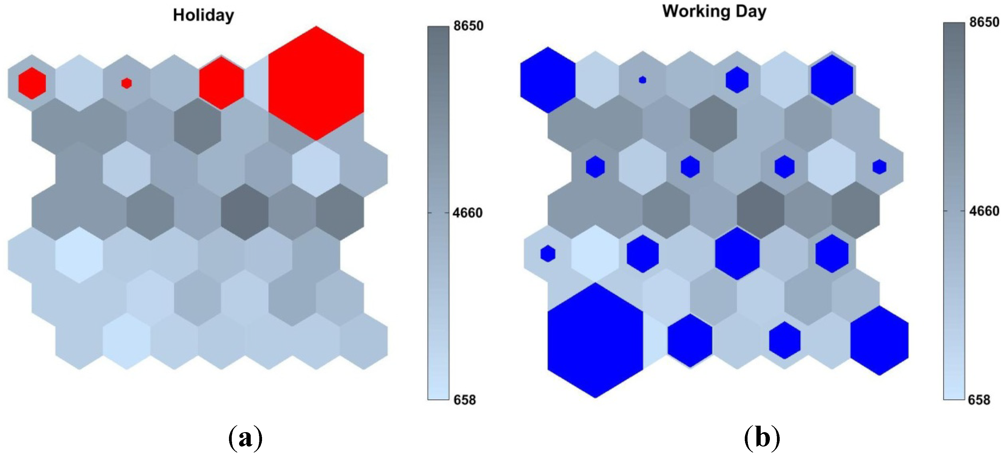
4.1. Classification with Self-Organizing Map

The SOM employed uses a 4 × 4 neuron architecture. The figures in this section (Figure 5, Figure 6 and Figure 7) represent the links among the neurons as well, so a 7 × 7 grid is presented in which each neuron cell is connected to other neuron cell by a link cell. For instance, in the top row, there are four neurons linked by three links, and the second row is populated only with the eight links binding the neurons in the first and third rows. The coloured hexagons represent the input patters that have been classified under each neuron: the bigger the coloured hexagon, the larger the number of patters assigned to that neuron.

After processing the data with the SOM, the resulting output clusters are presented in the following figures and analyzed according four different criteria for simplicity of interpretation and understanding:

• First, the clusters are shown in Figure 4 separated according the workability of the days. The left part of the image shows how non-working days were clustered, and the right part presents how working days were clustered.
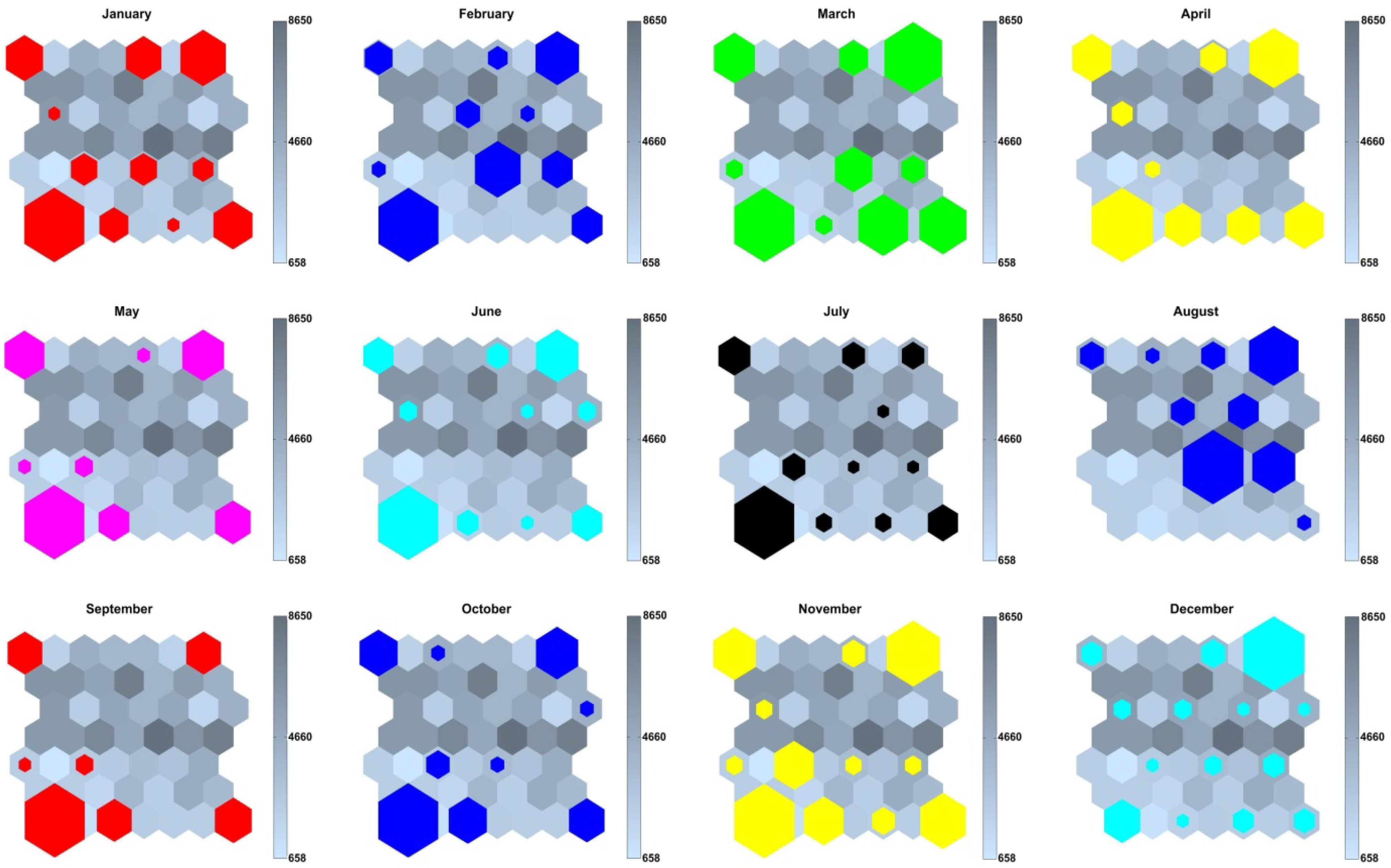
• Figure 5 shows how the days of the different months were clustered. It is easy to see that January, February and March activate similar neurons; April, May, June and July also form a group of similar activations, as September, October and November do; August and December are both of them isolated. This makes sense, as seasons are roughly outlined, together with summer holidays (August) and Christmas (December). Electricity demand is seasonally dependent, as shown by Hernández et al. [27].
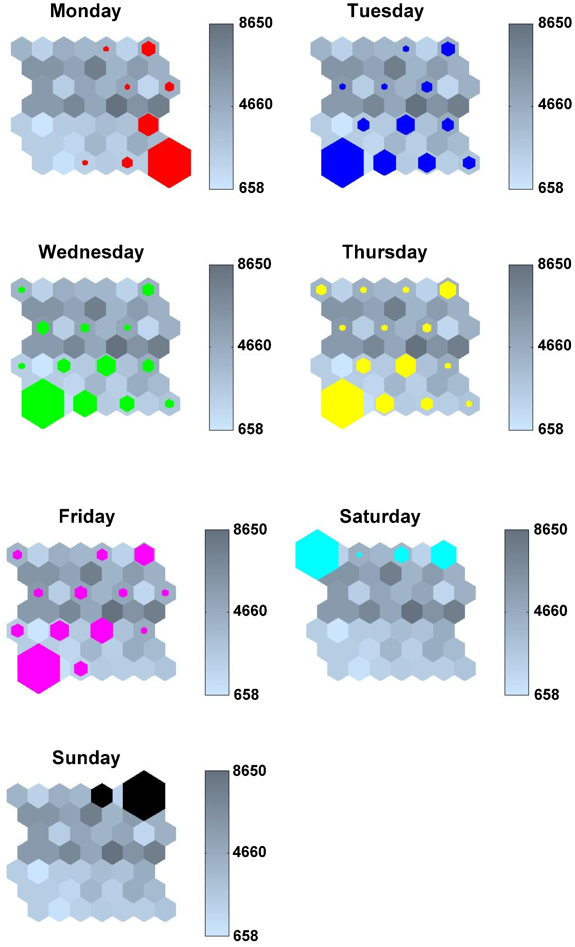
• Figure 6 presents how the different days of the week were clustered, resulting in four different patterns of activation: Mondays have their own activation pattern; Tuesday, Wednesday, Thursday and Friday have similar activation patterns; Saturdays and Sundays have again their own differentiated activation patterns.
• Finally, Figure 7 presents a combined analysis of clusters by day of the week and workability. All holidays are clustered around neurons similar to those of Sunday, except Wednesdays and Thursdays.

Figure 4. Activation map for workability: (a) non-working days; (b) working days.

Figure 4. Activation map for workability: (a) non-working days; (b) working days.

Figure 5. Activation map for months.

Figure 5. Activation map for months.

Figure 6. Activation map for weekdays.

Figure 6. Activation map for weekdays.

Figure 7. Activation map for workability and weekdays.

Figure 7. Activation map for workability and weekdays.

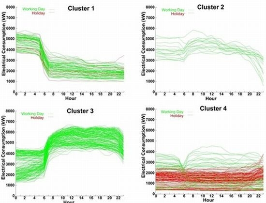
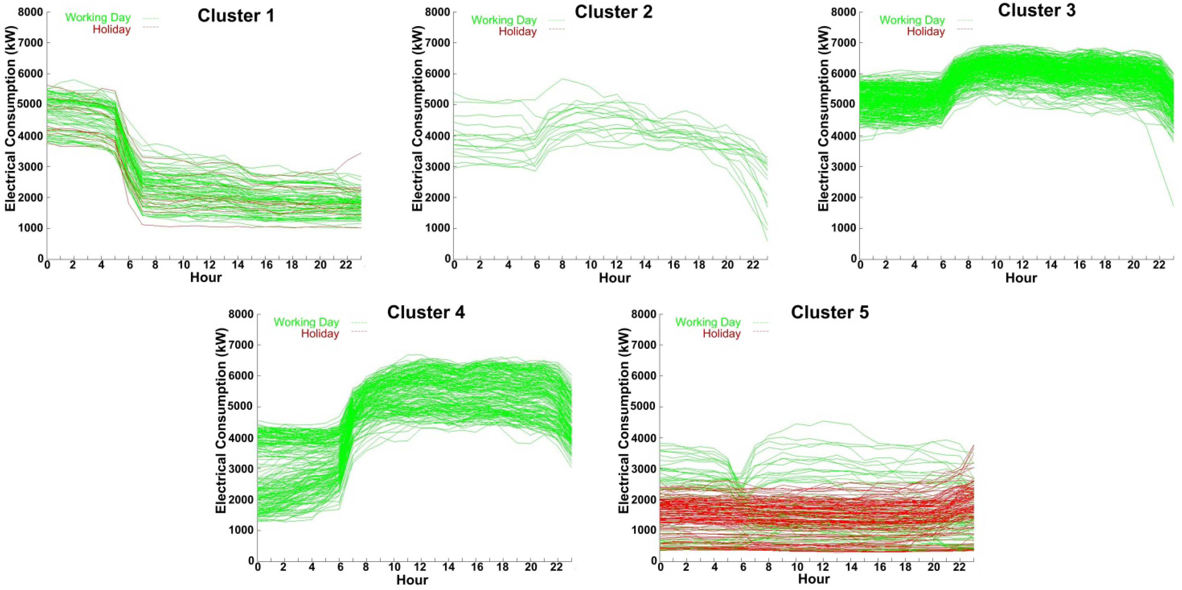
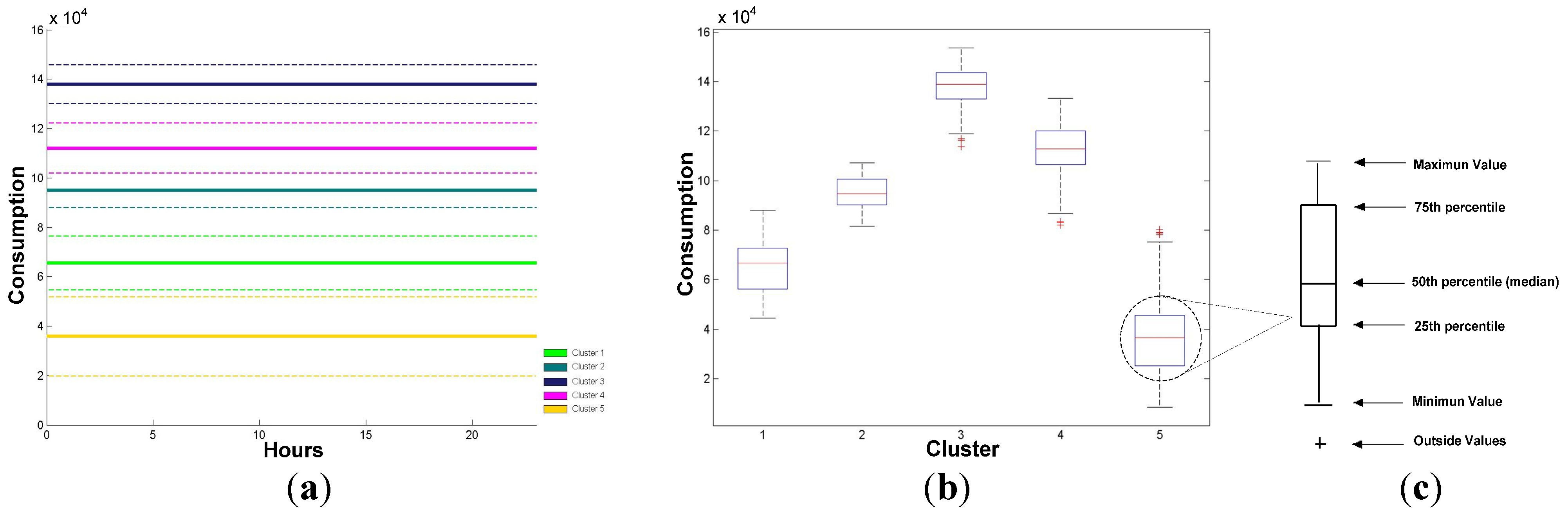
4.2. Clustering with k-Means

The results of the different evaluations of the clusters given by k-means show that the optimal number of clusters is five. Figure 8 presents all the curves belonging to each of the five clusters. It is easy to see the high similarity between curves of the same cluster, and the appreciable difference when compared with those of the other clusters.

Figure 8. Load curves for the five clusters, red curves are from holidays, and green days are working days.

Figure 8. Load curves for the five clusters, red curves are from holidays, and green days are working days.

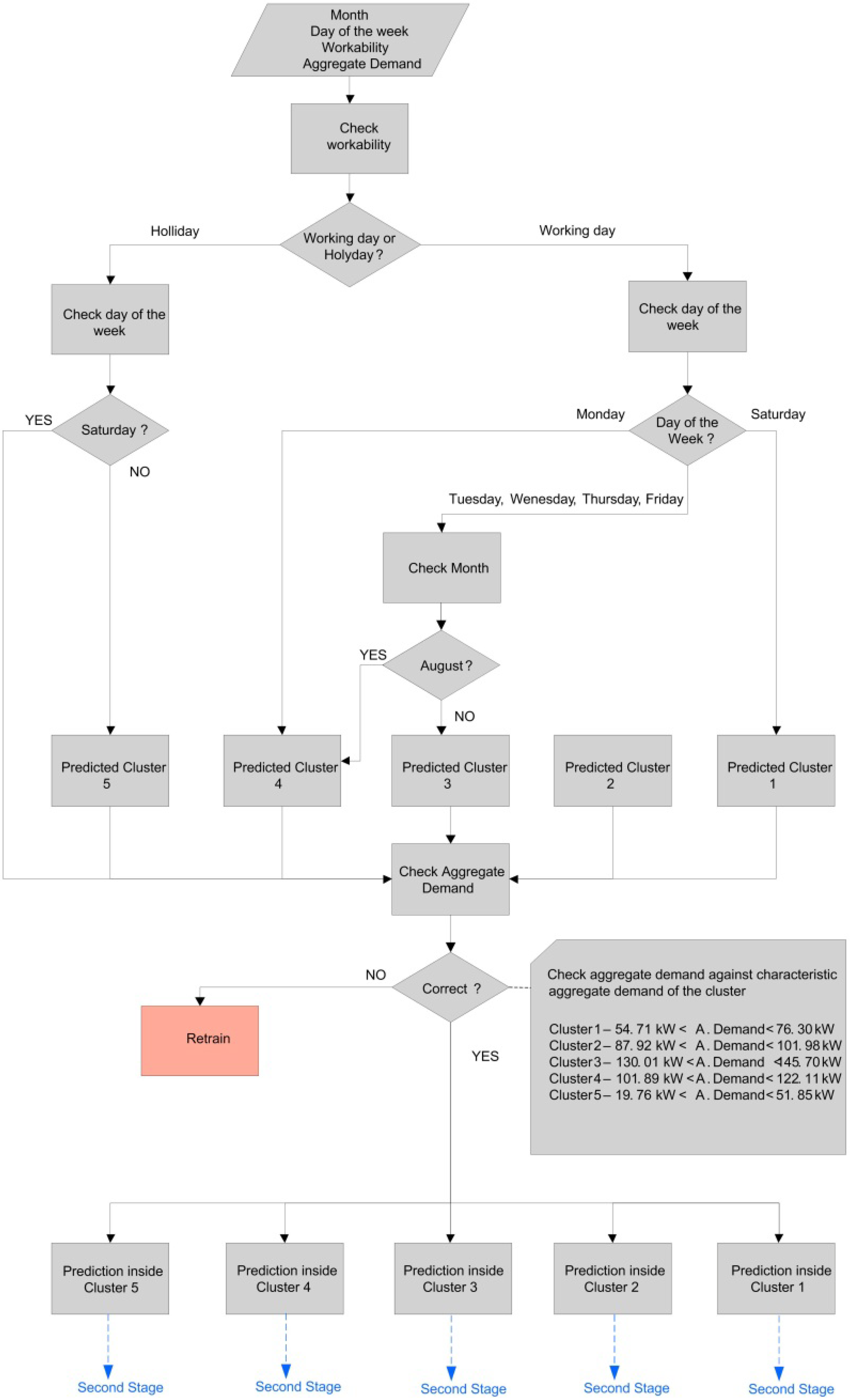
4.3. Decision Algorithm

Following the above results, Table 1 and Figure 9 present an analysis of the accumulated daily consumption per cluster.

Figure 9. (a) Average aggregate load ± standard deviation (the y-axis shows values of power consumption in W and the x-axis 24 hours per day); (b) box plot (the y-axis presents values of power consumption in W across the five clusters in the x-axis); (c) box plot legend.

Figure 9. (a) Average aggregate load ± standard deviation (the y-axis shows values of power consumption in W and the x-axis 24 hours per day); (b) box plot (the y-axis presents values of power consumption in W across the five clusters in the x-axis); (c) box plot legend.

Figure 10 shows a decision algorithm designed to control when the systems need to be retrained due to changes in the load curve behaviour. Basically, retraining is triggered when the aggregated demand for a day is outside the margins of the aggregate demand of the cluster inside it has been grouped.

Figure 10. Decision Algorithm.

Figure 10. Decision Algorithm.

Table 1. Analysis of results per cluster.

Number of cluster	Day of the week	Month	Workability	Average consumption (kW)
Cluster 1	Saturday	Indifferent	Working Day	4000 < Consumption
	Saturday		Holiday
Cluster 2	Indifferent	Indifferent	Working Day	4000
Cluster 3	Tuesday	Not August	Working Day	4000 < Consumption < 6000
	Wednesday
	Thursday
	Friday
Cluster 4	Monday	Indifferent	Working Day	1500 < Consumption < 4500
	Tuesday	August
	Wednesday
	Thursday
	Friday
Cluster 5	Monday	Indifferent	Holiday	Consumption < 4000
	Tuesday
	Wednesday
	Thursday
	Friday
	Saturday
	Sunday
	Saturday	Indifferent	Working Day	Consumption < 4000

Table 1. Analysis of results per cluster.

Number of cluster	Day of the week	Month	Workability	Average consumption (kW)
Cluster 1	Saturday	Indifferent	Working Day	4000 < Consumption
	Saturday		Holiday
Cluster 2	Indifferent	Indifferent	Working Day	4000
Cluster 3	Tuesday	Not August	Working Day	4000 < Consumption < 6000
	Wednesday
	Thursday
	Friday
Cluster 4	Monday	Indifferent	Working Day	1500 < Consumption < 4500
	Tuesday	August
	Wednesday
	Thursday
	Friday
Cluster 5	Monday	Indifferent	Holiday	Consumption < 4000
	Tuesday
	Wednesday
	Thursday
	Friday
	Saturday
	Sunday
	Saturday	Indifferent	Working Day	Consumption < 4000

5. Conclusions and Future Works

The data analysis system presented in this work has been tested and validated using real world data. In the results, the daily consumption behaviour of a real industrial park has been analyzed by clustering the different days according to their load curves, and meaningful behaviour patterns have been properly identified by the system in a completely unsupervised fashion. This shows that the system is actually capable of providing very useful information about the consumption patterns in disaggregated, small scale energy environments. As discussed, the system described represents an important step over the current state of the art in identification of patterns in demand curves, which was rich in applications over large areas (such as regions or nations), but not in microgrid-sized environments. These environments are not only a different application scenario from the typical case, but also a more difficult one due to the increased variability in the demand curve caused by a smaller aggregation with less atomic entities contributing to the curve to be studied.

References

1. Optimagrid: The Project Aims to Define, Design, Develop and Implement Intelligent Control Systems of Energy That Facilitate the Management Real-Time of a Microgrid. Available online: http://www.optimagrid.eu/ (accessed on 20 February 2012).
2. Hingorani, N.G. Introducing custom power. IEEE Spectr. 1995, 32, 41–48. [Google Scholar] [CrossRef]
3. Liserre, M.; Sauter, T.; Hung, J.Y. Future energy systems: Integrating renewable energy resources into smart power grid through industrial electronics. IEEE Ind. Electron. Mag. 2010, 4, 18–37. [Google Scholar] [CrossRef]
4. Halpin, S.M.; Smith, J.W.; Litton, C.A. Designing industrial systems with a weak utility supply. IEEE Ind. Electron. Mag. 2001, 7, 63–70. [Google Scholar] [CrossRef]
5. Xinghuo, Y.; Cecati, C.; Dillon, T.; Simoes, M.G. The new frontier of smart grids. IEEE Ind. Electron. Mag. 2011, 5, 49–63. [Google Scholar]
6. Santacana, E.; Rackliffe, G.; Tang, L.; Feng, X. Getting smart. IEEE Power Energy Mag. 2010, 8, 41–48. [Google Scholar] [CrossRef]
7. Park, J.-I. A smart factory operation method for a smart grid. In Proceedings of the 2010 40th International Conference on Computers and Industrial Engineering (CIE), Awaji City, Japan, 25–28 July 2010.
8. Zareipoor, H.; Cañizares, C.A.; Bhattacharga, K. Economic impact of electricity market price forecasting errors: A demand-side analysis. IEEE Tran. Power Syst. 2010, 25, 254–262. [Google Scholar] [CrossRef]
9. Vaccaro, A.; Popou, M.; Villacci, D.; Terzija, V. An integrated framework for smart microgrids modelling, monitoring, control, communication, and verification. Proc. IEEE 2011, 99, 119–132. [Google Scholar] [CrossRef]
10. García, J.L.; Blasco, J.A.; del Brío, M.B.; Dominguez, J.A.; Barquillas, J.; Ramirez, I.J.; Medrano, N.J. Short-term electric power load-forecasting using artificial neural networks. Part I: Self-organizing networks for classification of day types. In Proceedings of the Fourteenth IASTED International Conference Modelling, Identification and Control, Igls, Austria, 20–22 February 1995; IASTED (International Association of Science and Technology for Development): Alberta, Canada, 1995; pp. 218–222. [Google Scholar]
11. García, J.L.; Blasco, J.A.; del Brío, M.B.; Dominguez, J.A.; Barquillas, J.; Ramirez, I.J.; Medrano, N.J. Short-term electric load-forecasting using ANN. Part II: Multilayer perception for hourly electric-demand forecasting. In Proceedings of the Fourteenth IASTED International Conference Modelling, Identification and Control, Igls, Austria, 20–22 February 1995; IASTED (International Association of Science and Technology for Development): Alberta, Canada, 1995; pp. 223–227. [Google Scholar]
12. Marín, F.J.; García-Lagos, F.; Joya, G.; Sandoval, F. Global model for short-term load forecasting using artificial neural networks. IEE Proc Gener. Transmi. Distrib. 2002, 149, 121–125. [Google Scholar] [CrossRef]
13. Mori, H.; Itagaki, T. A precondition technique with reconstruction of data similarity based classification for short-term load forecasting. In Proceedings of 2004 IEEE Power Engineering Society General Meeting, Denver, CO, USA, 6–10 June 2004.
14. Carpinteiro, O.A.S.; Reis, A.J.R. A SOM-based hierarchical model to short-term load forecasting. In Proceedings of 2005 IEEE Russia Power Tech, St. Petersburg, Russia, 27–30 June 2005.
15. Wang, Z.Y. Development case-based reasoning system for short-term load forecasting. In Proceedings of 2006 IEEE Russia Power Engineering Society General Meeting, Montreal, Canada, 18–22 June 2006.
16. George, T.J.; Hatziargyriou, N.D.; Dialynas, E.N. Two-stage pattern recognition of load curves for classification of electricity customers. IEEE Trans. Power Syst. 2007, 22, 1120–1128. [Google Scholar] [CrossRef]
17. Chicco, G.; Napoli, R.; Piglione, F.; Postolache, P.; Scutariu, M.; Toader, C. Load pattern-based classification of electricity customers. IEEE Trans. Power Syst. 2004, 19, 1232–1239. [Google Scholar] [CrossRef]
18. Kohonen, T. The Self-organizing Map. Proc. IEEE 1990, 78, 1464–1480. [Google Scholar] [CrossRef]
19. Kohonen, T. Self-organized formation of topologically correct feature maps. Biol. Cybern. 1982, 43, 59–69. [Google Scholar] [CrossRef]
20. Kohonen, T. Analysis of a simple self-organizing process. Biol. Cybern. 1982, 44, 135–140. [Google Scholar] [CrossRef]
21. Kohonen, T. The neural phonetic typewriter. IEEE Comput. Mag. 1988, 21, 11–22. [Google Scholar] [CrossRef]
22. MacQueen, J.B. Some methods for classification and analysis of multivariate observations. In Proceedings of the 5th Berkeley Symposium on Mathematical Statistics and Probability, Berkeley, CA, USA, 18–21 July 1967; University of California Press: Berkeley, CA, USA, 1967; pp. 281–297. [Google Scholar]
23. Vesanto, J.; Alhoniemi, E. Clustering of the self-organizing map. IEEE Trans. Neural Netw. 2000, 11, 586–600. [Google Scholar] [CrossRef] [PubMed]
24. López, M.; Valero, S.; Senabre, C.; Aparicio, J. A SOM neural network approach to load forecasting. Meteorological and time frame influence. In Proceedings of the 2011 International Conference on Power Engineering and Electrical Drivers, Málaga, Spain, 11–13 May 2011.
25. Hsu, Y.-Y.; Yang, C.-C. Design of artificial neural networks for short-term load forecasting. Part I: Self-organising feature maps for day type identification. IEE Proc. C Gener. Transm. Distrib. 1991, 138, 407–413. [Google Scholar]
26. Davies, D.L.; Bouldin, D.W. A cluster separation measure. IEEE Trans. Pattern Anal. Mach. Intell. 1979, PAMI-1, 224–227. [Google Scholar]
27. Hernández, L.; Baladrón, C.; Aguiar, J.M.; Calavia, L.; Carro, B.; Sánchez-Esguevillas, A.; Cook, D.J.; Chinarro, D.; Gómez, J. A study of the relationship between weather variables and electric power demand inside a smart grid/smart world framework. Sensors 2012, 12, 11571–11591. [Google Scholar] [CrossRef]