A Novel Data-Driven Fast Capacity Estimation of Spent Electric Vehicle Lithium-ion Batteries

Abstract

Fast capacity estimation is a key enabling technique for second-life of lithium-ion batteries due to the hard work involved in determining the capacity of a large number of used electric vehicle (EV) batteries. This paper tries to make three contributions to the existing literature through a robust and advanced algorithm: (1) a three layer back propagation artificial neural network (BP ANN) model is developed to estimate the battery capacity. The model employs internal resistance expressing the battery’s kinetics as the model input, which can realize fast capacity estimation; (2) an estimation error model is established to investigate the relationship between the robustness coefficient and regression coefficient. It is revealed that commonly used ANN capacity estimation algorithm is flawed in providing robustness of parameter measurement uncertainties; (3) the law of large numbers is used as the basis for a proposed robust estimation approach, which optimally balances the relationship between estimation accuracy and disturbance rejection. An optimal range of the threshold for robustness coefficient is also discussed and proposed. Experimental results demonstrate the efficacy and the robustness of the BP ANN model together with the proposed identification approach, which can provide an important basis for large scale applications of second-life of batteries.

1. Introduction

The number of electric vehicles (EVs) and plug-in hybrid electric vehicles (PHEV) has been growing at a rapid rate in recent years driven by the need to curb air pollution caused by petroleum-based vehicles. As a result, it is expected that a large number of “spent” electric vehicle batteries will become available. These batteries will have capacities in the range of 70%–80% of their initial value, which may not be acceptable for electric vehicle use, but may be usable in other less demanding applications, in terms of energy density requirements, such as grid reinforcement or buffering of intermittent renewable energy sources. This could in turn help reduce the cost of power batteries used in EVs, thus paving the way for faster EV development.

In recent years, research on the re-use of spent EV, PHEV batteries has focused on reliability estimation [1], optimal use strategy [2] and economic analysis [3,4]. Mukherjee et al. [1] presented a reliability calculation method for a battery energy storage system, and designed a battery-to-grid converter topology for robust and reliable second-life batteries. Rule-based control is used to manage the charging and discharging of second-life batteries to extend their lifetime in [2], and realize commercial building peak load management and maximize cost savings. Neubauer and Pesaran [3] assessed the impact of the use of second-life batteries on the initial cost of PHEV/EV batteries to automotive consumers. They concluded that although the battery re-use is not expected to significantly affect today’s PHEV/EV prices, it has the potential to transform markets in need of cost-effective energy storage.

Most of the above papers assume that the battery parameters are known. However, significant work is needed to characterize second-life batteries. Battery parameters including Ohmic resistance, polarization impedance and available capacity are needed. The available capacity, which describes the total capacity from a battery at a specified operation condition, is a key parameter in second-life battery applications. The parameters of a second-life battery will in general depend on their usage history. Batteries used under similar operating conditions and with a similar usage history tend to generally degrade at a similar rate and hence will have similar parameters. The battery capacity distribution characters used in two EV buses run at the same route are illustrated in Figure 1. It is shown that the parameters of the spent batteries used on EV buses applied in certain routes seem to have approximately identical statistical characteristics.

Commonly used methods for estimating available capacity include the full charge-discharge method, open circuit voltage (OCV) [5], load voltage [6], internal resistance acquisition [7], extended Kalman filter (EKF)-based estimation [8,9,10,11], and statistical learning methods such as support vector machines (SVMs) [12] and artificial neural networks (ANNs) [13,14,15,16,17]. Among them, full charge-discharge measurement is an accurate and reliable method. It is however time consuming and costly, and difficult to achieve for a large number of spent EV batteries. In [5], the unique OCV-Specific gravity relation that exists in lead-acid types was used to realize an estimation of the battery remaining capacity, but this technique is not suitable for lithium-ion batteries. A unified discharge voltage characteristic was presented to estimate battery capacity in [6]. The proposed method was simple to implement, however, it required a lot of experiments to characterize battery discharge behaviors. EKF and its improved algorithm based on various lumped parameter battery models were reported in [8,9,10,11]. The method can provide accurate estimation with model inaccuracy and measurement noises. However, it is a recursive method and needs historic data to get estimate updates, which is not practical for the estimation of hundreds of battery cells. The statistical learning methods aim to learn the behavior of the studied system from a large number of examples and then find a mathematical system description [12]. Such statistical methods can be employed without knowledge of battery internal structure and usage history, so long as training data is available [18]. SVM finds the solution to the support vector based on quadratic programming, which suffers from the need for large sample training. The ANN algorithm on the other hand has an advantage of parallel processing for large scale data. When comparing the existing ANN methods for battery life estimation, we find that most of them are used for battery cells and less for battery systems containing ten to hundreds of battery cells. This study aims to investigate the viability and effectiveness of ANN for estimating the available capacity of spent second-life EV lithium ion batteries that have been used on EV buses.

Figure 1. Statistics of the battery capacity for two electric vehicle (EV) buses.

Figure 1. Statistics of the battery capacity for two electric vehicle (EV) buses.

The paper is organized as follows: in Section 1 it is demonstrated that the used battery parameters of EV buses with the same usage history have identical statistical properties, which is the basis for parameter estimation using the ANN algorithm. A back propagation artificial neural network (BP ANN) model is then introduced as a basis for capacity estimation, in which the internal resistances with various currents at particular time points are used as inputs to the model. This part is discussed in Section 2. In Section 3, the BP ANN model is trained to get an accurate estimation of the battery capacity. The robustness of the model is then discussed in detail. Taking model accuracy and robustness into consideration a robust BP ANN modeling method is proposed. The basic method and principle of choosing the robustness coefficient is also discussed. The verification of the proposed method is then presented in Section 4. The conclusions are finally summarized in Section 5.

2. Back Propagation Network Modeling of a Battery System

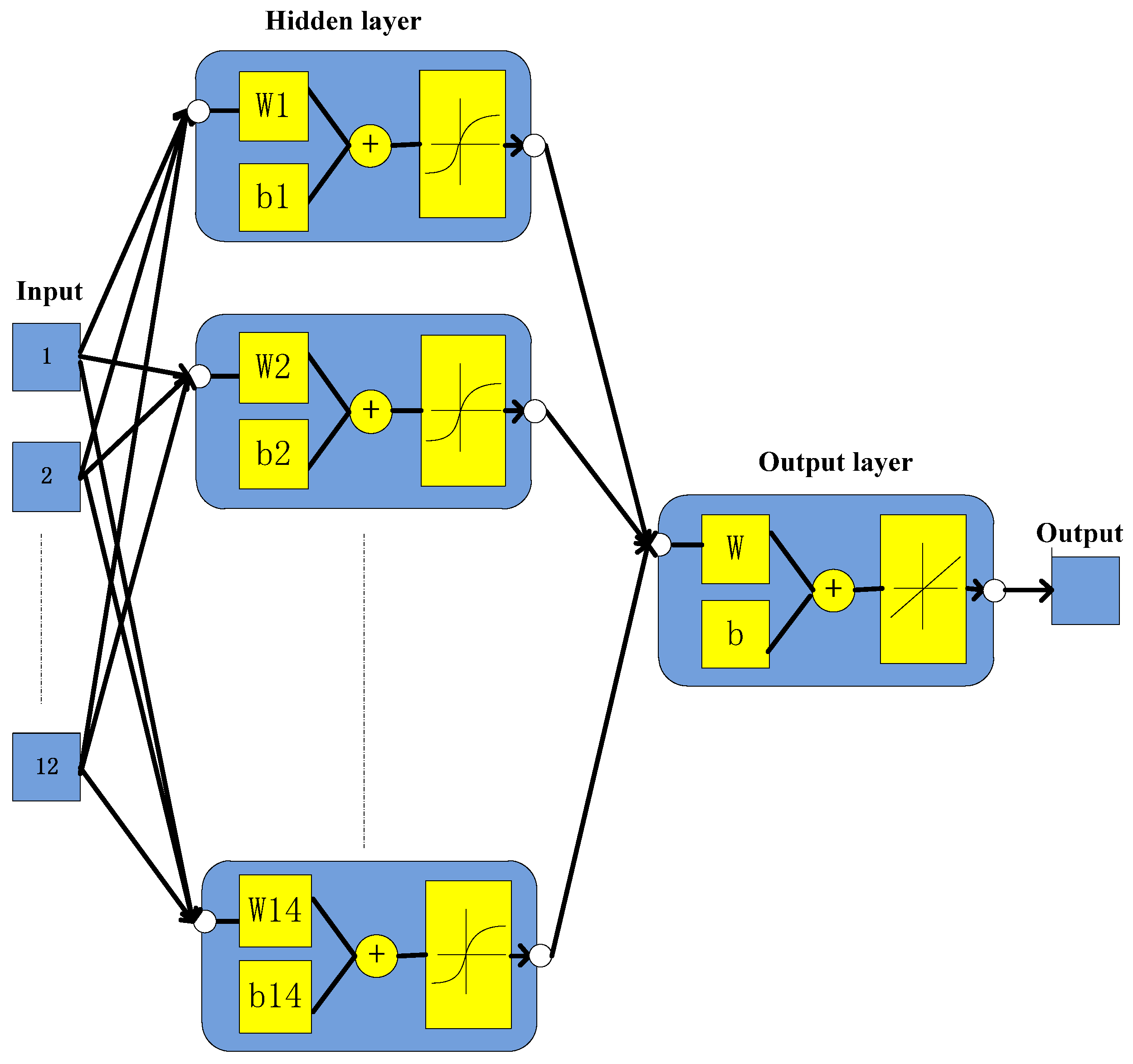
2.1. The Model Structure

The feed-forward neural networks are classical ANN architectures, of which the BP network is commonly used since it has the ability to achieve nonlinear mapping, self-learning and adaptive, and generalization [19]. We started with a popularly used BP neural network with three layers comprising one input layer, one hidden layers and one output layer. It is demonstrated that the model with three layers has acceptable accuracy. The structure of the BP network is shown in Figure 2.

Figure 2. The structure of the back propagation artificial neural network (BP ANN) model.

Figure 2. The structure of the back propagation artificial neural network (BP ANN) model.

The impedance and capacity degradation of the batteries between EV buses are relatively analogous since the battery packs were placed in the same location in the EV buses. Researchers have reported that the impedance of a lithium-ion battery is related to its state of charge (SOC) and state of health (SOH) [20,21], which are used to identify the battery aging mechanism. The internal resistance obtained from the voltage response of the battery at pulse current can in part describe the battery kinetics. This is consistent with the impedance obtained using an electrochemical impedance spectroscopy (EIS) test. It is therefore reasonable to estimate the capacity based on the internal resistance of the battery. Hence, the internal resistance, measured during pulsed current tests and at different sampling times is employed as an input to the capacity estimating neural network.

Taking the available charge/discharge currents and polarization time constant of the sample batteries into consideration, three currents and four sampling times are finally selected. The ANN model in this study therefore includes 12 training inputs, and each input is a column vector. The twelve vectors contain the batteries’ internal resistances acquired by pulse currents response of −200 A, −300 A and 100 A (discharge current is negative in this paper) at various sampling time which are 0.5, 1, 5 and 10 s. The output is the capacity of the batteries.

In the hidden layer, a bipolar sigmoid transfer function is used, since it is continuously differentiable, and in which the weights from input to hidden units can be adjusted based on backward propagation of errors learning algorithm. The bipolar sigmoid function is given by:

$$f(v)=\frac{1-{\text{e}}^{-\text{λ}v}}{1+{\text{e}}^{-\text{λ}v}}$$

(1)

where $v_i={\displaystyle \sum _{j=1}^{12}{w}_{ij}\ast p_j}+b_i$, p_j represents the jth input vector, w_ij is the weights value of the input vector p_j, b_i is biases values of the ith neuron. After analyzing the model input and output architecture, various numbers of neurons were trained; the neuron number in the hidden layer was determined to be 14 taking model accuracy and generalization abilities into account [22].

The mean square error (MSE) of the network output compared to the target is adopted as the error function. The goal is to minimize the average of the sum of the square of the errors:

$$MSE=\frac{1}{N}{\displaystyle \sum }_{i=1}^N{(Q_i^{\text{e}}-Q_i^{\text{t}})}^2$$

(2)

where $Q_i^{\text{t}}$ is the experimental capacity value of cell i, $Q_i^{\mathrm{e}}$ is the estimated value of cell i, N represents the number of batteries used to train the ANN.

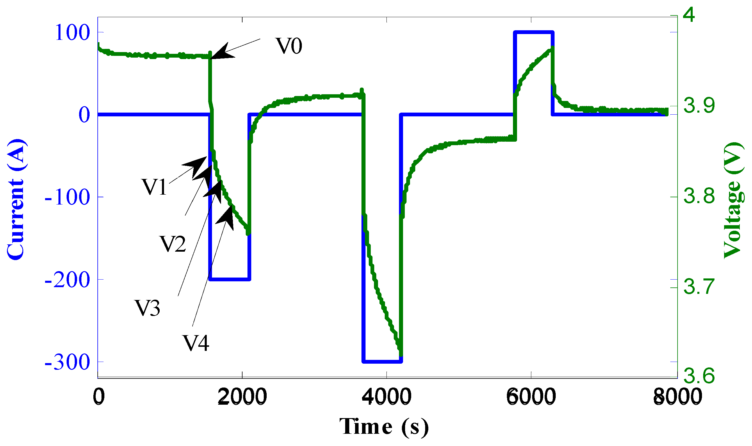
2.2. Input of the Back Propagation Model

As mentioned earlier, the battery internal resistances calculated at sampling times ranging from 0.5 to 10 s are employed as the model input since they can express battery dynamics such as Ohmic loss, activation polarization and concentration polarization. The dynamic resistance of the battery at the specified SOC and temperature can be determined experimentally based on the voltage response at the pulse current as illustrated above in Figure 3. The battery’s dynamic resistance R_i can be calculated as:

$$R_i=\frac{\left|V_i-V_0\right|}{\left|I_n\right|}$$

(3)

where I_n is the current measured at the sampling time. It is well known that the battery internal resistances in the middle region ranging from 20% to 80% SOC vary less than at both ends of the SOC [23], hence, the battery dynamic resistance in the middle range of SOC is applied in the study. Thus the kth input vector is given by:

$$R_k={[R_1,R_2,\cdots R_i,\cdots ]}^T,\begin{array}{cc}& \end{array}i=1,2,3,\cdots ,n$$

(4)

where n expresses the number of the tested batteries.

Figure 3. Voltage response at the pulse current.

Figure 3. Voltage response at the pulse current.

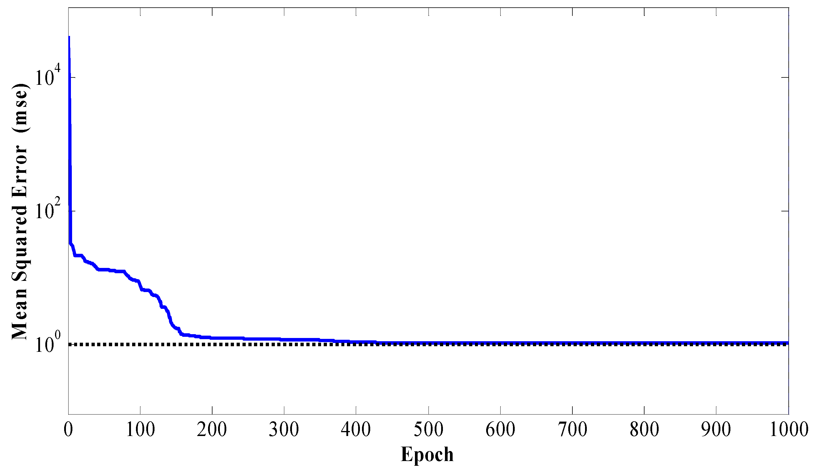
2.3. Method of Back Propagation Network Training

The basic principle of BP training relies on the gradient descent method, which can reduce the network error by altering the weights and bias values along the direction of the negative gradient [13]. In this study, the Levenberg-Marquardt (LM) algorithm, which is a variant of the gradient descent method, is used to optimize the network weight parameters. The LM method is a modification of classical Newton algorithm for optimum solution to a minimization problem, and is often described as a more stable and efficient method than a BP algorithm. It is also preferred due to its fast convergence and stability in training of ANNs [13].

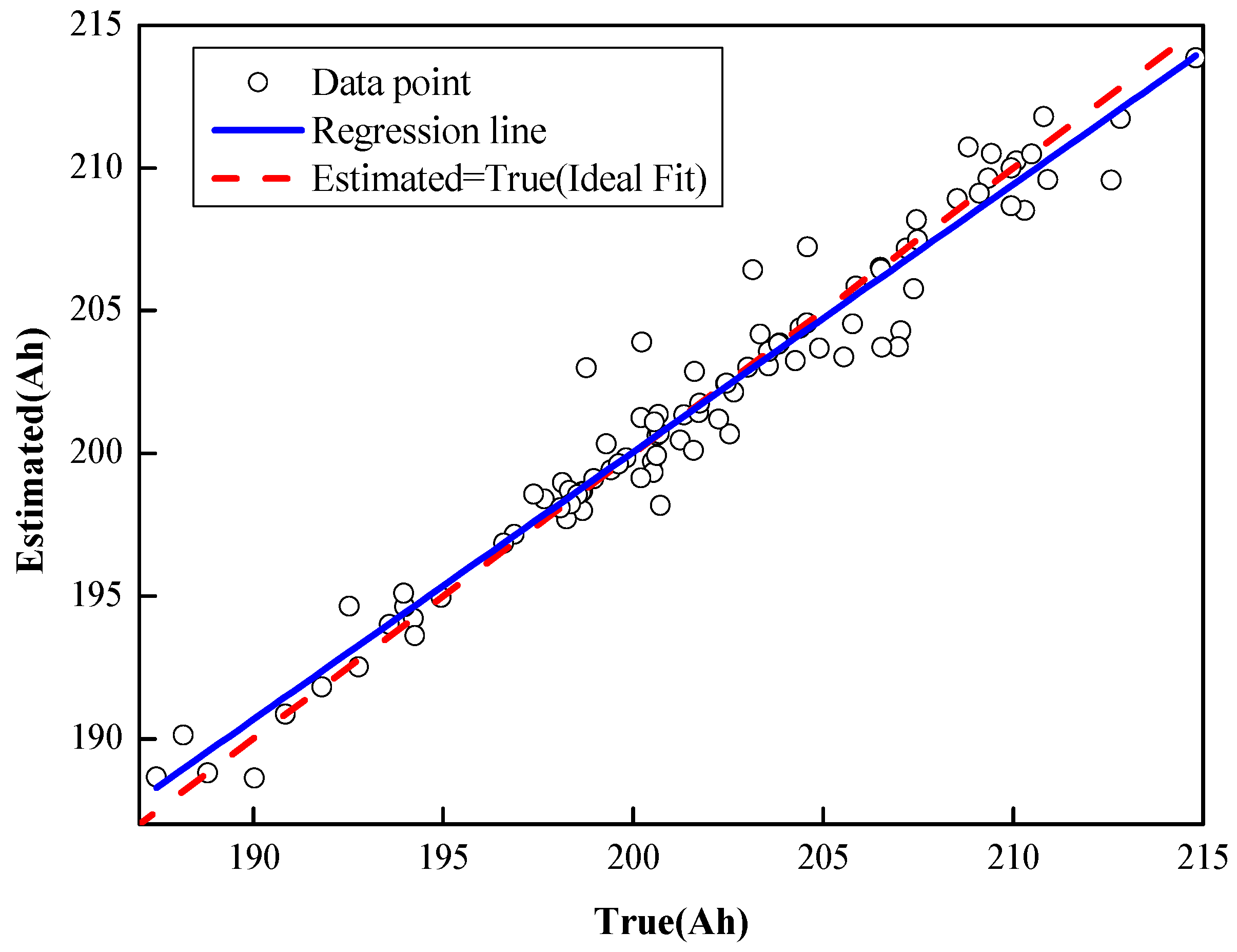
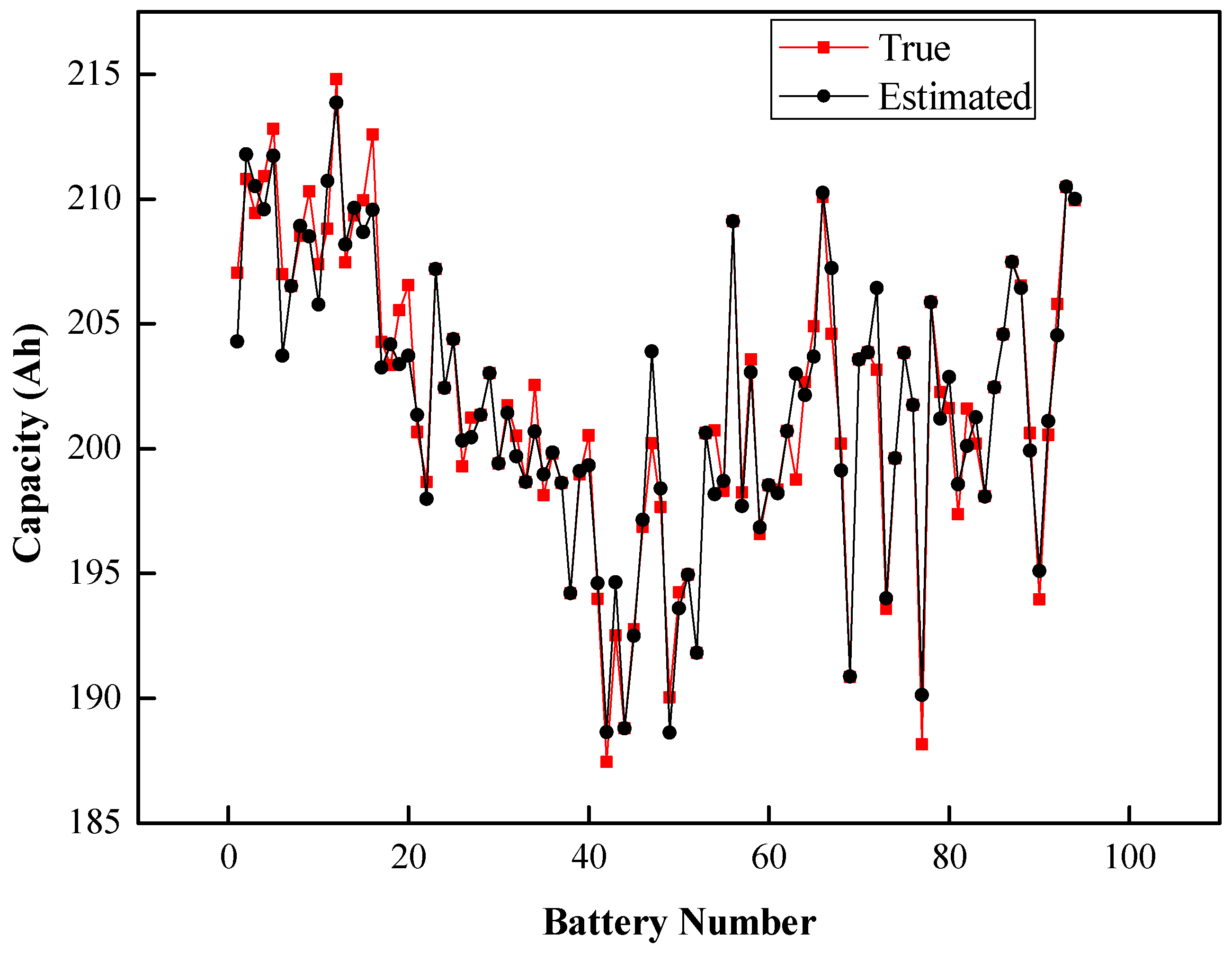
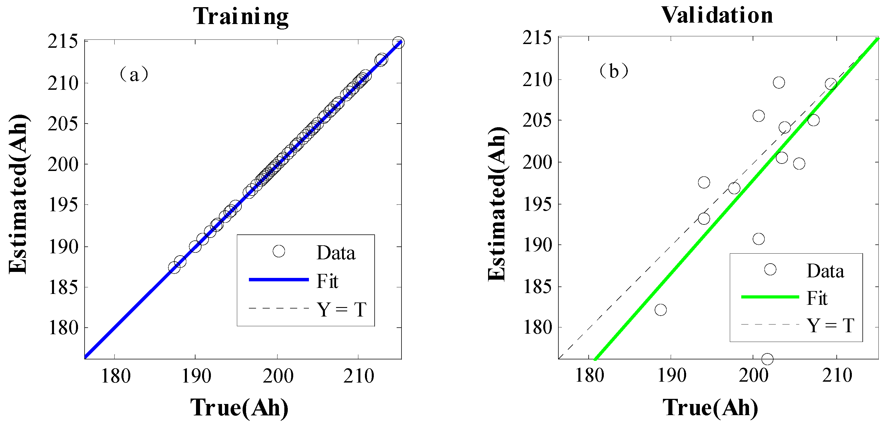
3. Available Capacity Estimation Using the Back Propagation Neural Network

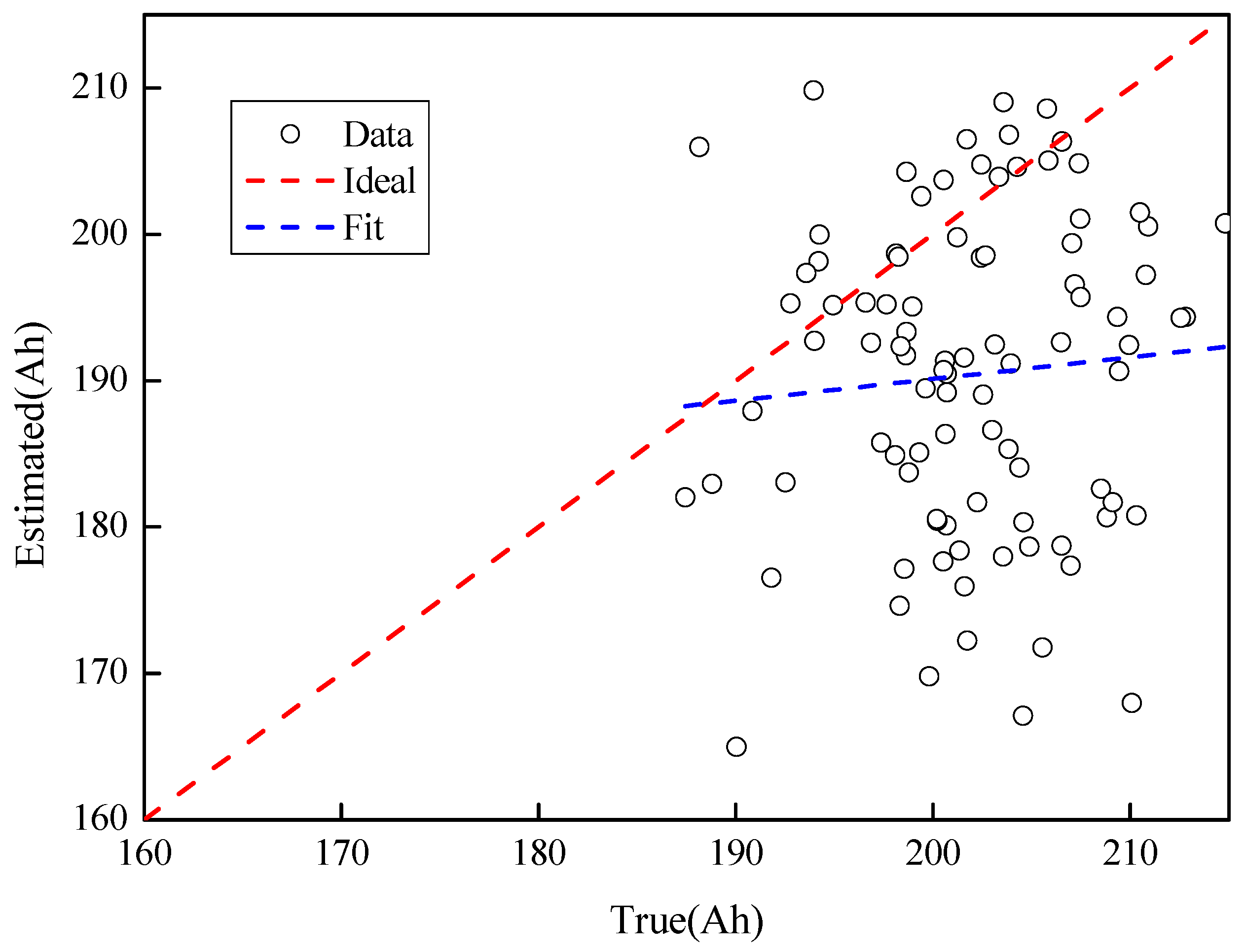
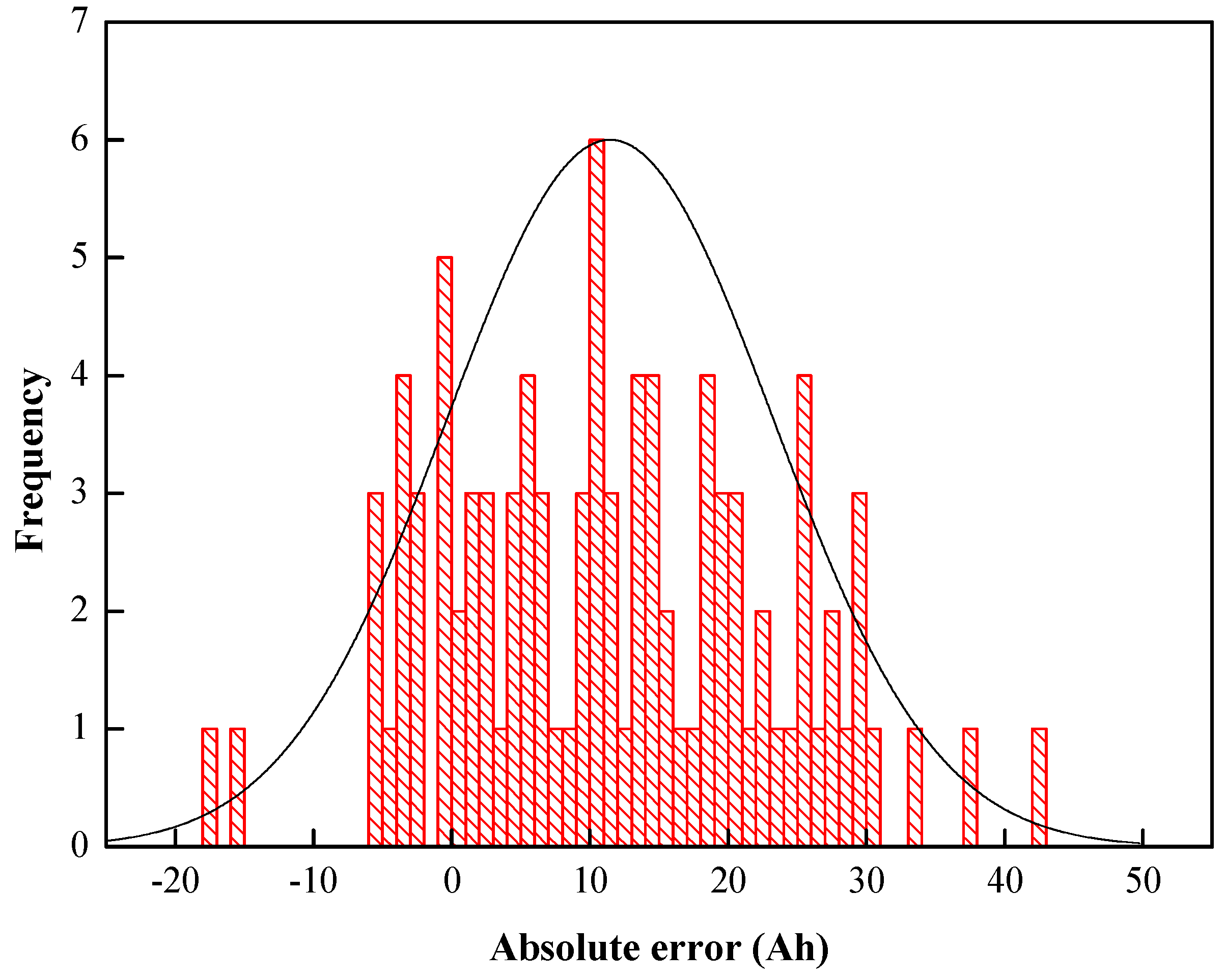
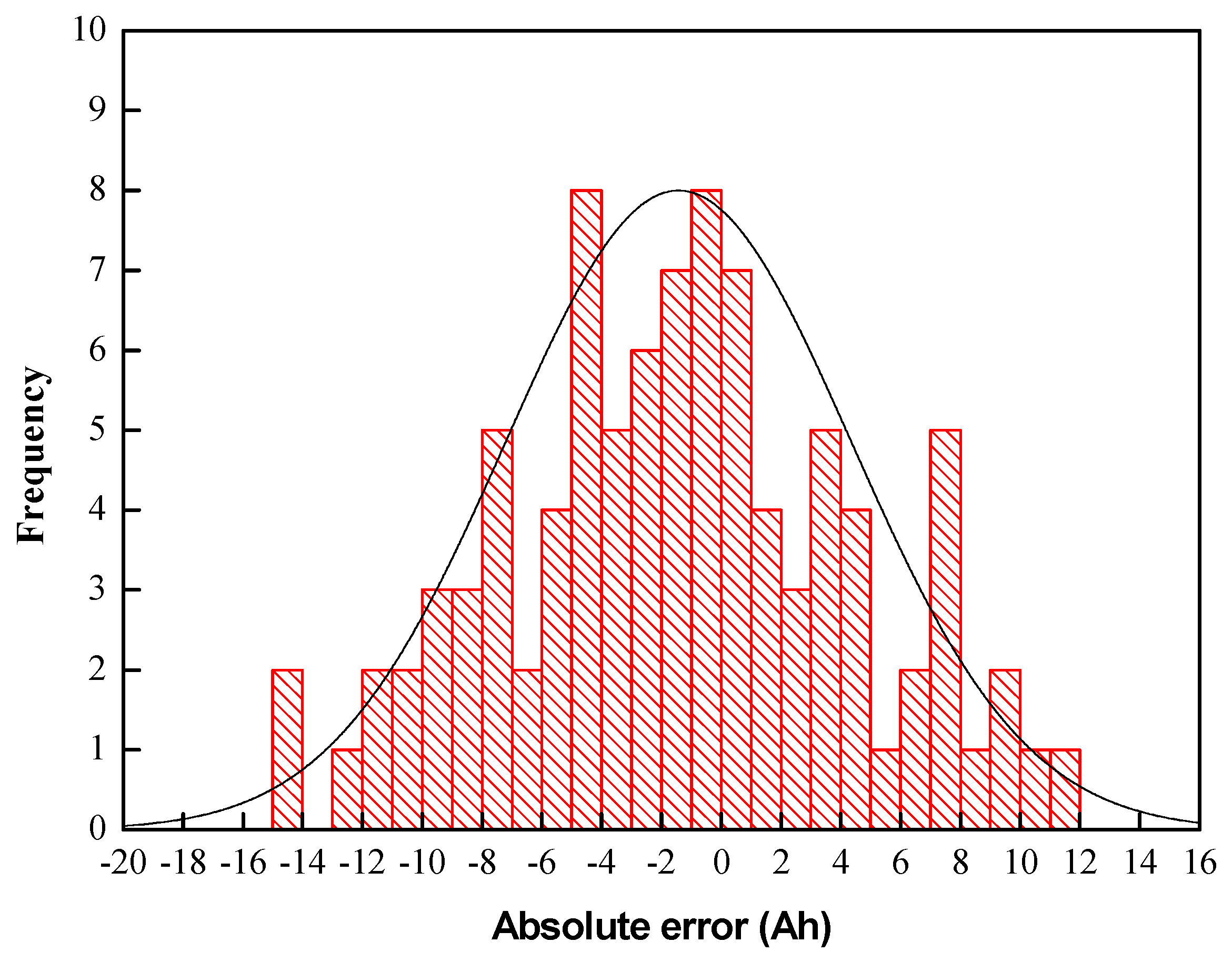
3.1. Training Result Analysis

Ninety fours batteries that were used on a Beijing Olympic EV bus were chosen as the training sample in this paper. The tested capacity of the batteries with full charge-discharge cycle ranged from 185 Ah to 215 A·h. The internal resistances, which were measured under 100 A, −200 A and −300 A pulsed current tests at 50% SOC with sampling time at 0.5, 1, 5 and 10 s, were used as inputs to the ANN, as mentioned earlier. The training parameters of the neural network model are set as target error e = 0.1, the maximum number of iterations is 1000 for once training cycle, and the initial weights and biases are random values in the [−0.1, 0.1] range.

The training error curve of the BP ANN model is shown in Figure 4. It can be seen that after 1000 iterations, the MSE does not achieve the designed target error 0.1; however, the error curve eventually becomes steady, indicating that the minimum stable MSE is approximately around 1. The error difference after training 600 times and 1000 times is negligible, therefore 600 iterations were considered sufficient to meet the BP neural network accuracy requirements.

Figure 4. Mean square error (MSE) of the model.

Figure 4. Mean square error (MSE) of the model.

To summarize the model accuracy statistics, the weights are randomized and the entire training performed 100 times. The statistics of MSE for 100 trainings is shown in Figure 5. It can be seen that the maximum MSE is around 7, suggesting that the average error is approximately 3.5%. The estimated and true values of the battery capacity and their linear regression relationship are shown in Figure 6. The true values were obtained using the full charge-discharge method. The abscissas of the data points in Figure 6 are the capacity true values (targets), and the corresponding ordinates are the capacity estimated values (model outputs). Ideally, the model output and the target values are equal to each other with all the data points falling on a straight line with slope equaling 1. The training regression coefficient is theoretically 1, which is represented by the dotted line in Figure 6. The calculated regression coefficient based on the data points is 0.968. The more accurate the model estimates, the closer the scatter of the data points to the solid regression line. In this case, the training regression line and the ideal fit line almost coincide, which suggested that the model output is consistent with the true values, and the BP neural network model is valid.

Figure 5. The MSE statistics for 100 training cycles.

Figure 5. The MSE statistics for 100 training cycles.

Figure 6. Linear regression relationship between model outputs and targets.

Figure 6. Linear regression relationship between model outputs and targets.

A comparison of estimated and true values is shown in Figure 7, and the absolute error distribution is illustrated in Figure 8, for 94 batteries. It can be seen in Figure 8 that the model absolute error approximately obeys a Gaussian distribution with an average of 0.899 A·h and a variance of 2.034 A·h. The maximum absolute error is 4.23 A·h, and the capacity estimation error is controlled within 2.5%. It indicates that the BP ANN has high estimation accuracy.

To test the model, 80% of the sample data is applied for the training model, and the remaining 20% of the data is used to validate the trained model. The comparisons of the trained and validated results are illustrated in Figure 9. It can be found that regression coefficient of validated results is around 0.91, indicating acceptable estimation accuracy.

Figure 7. Comparisons of the estimated and true values.

Figure 7. Comparisons of the estimated and true values.

Figure 8. Statistical characters of absolute errors between model outputs and targets.

Figure 8. Statistical characters of absolute errors between model outputs and targets.

Figure 9. Comparisons of the trained and validated results. (a): Trained results; (b): validated results.

Figure 9. Comparisons of the trained and validated results. (a): Trained results; (b): validated results.

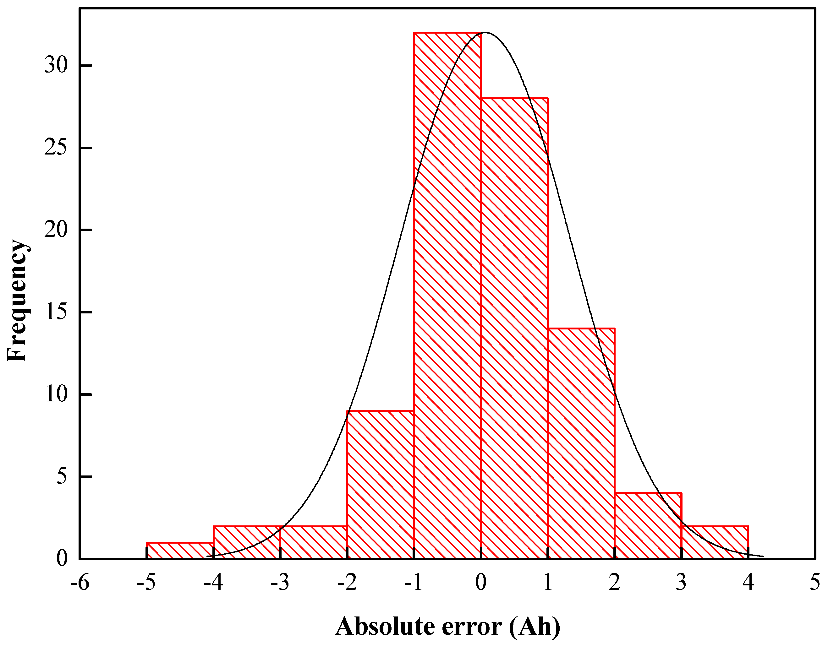
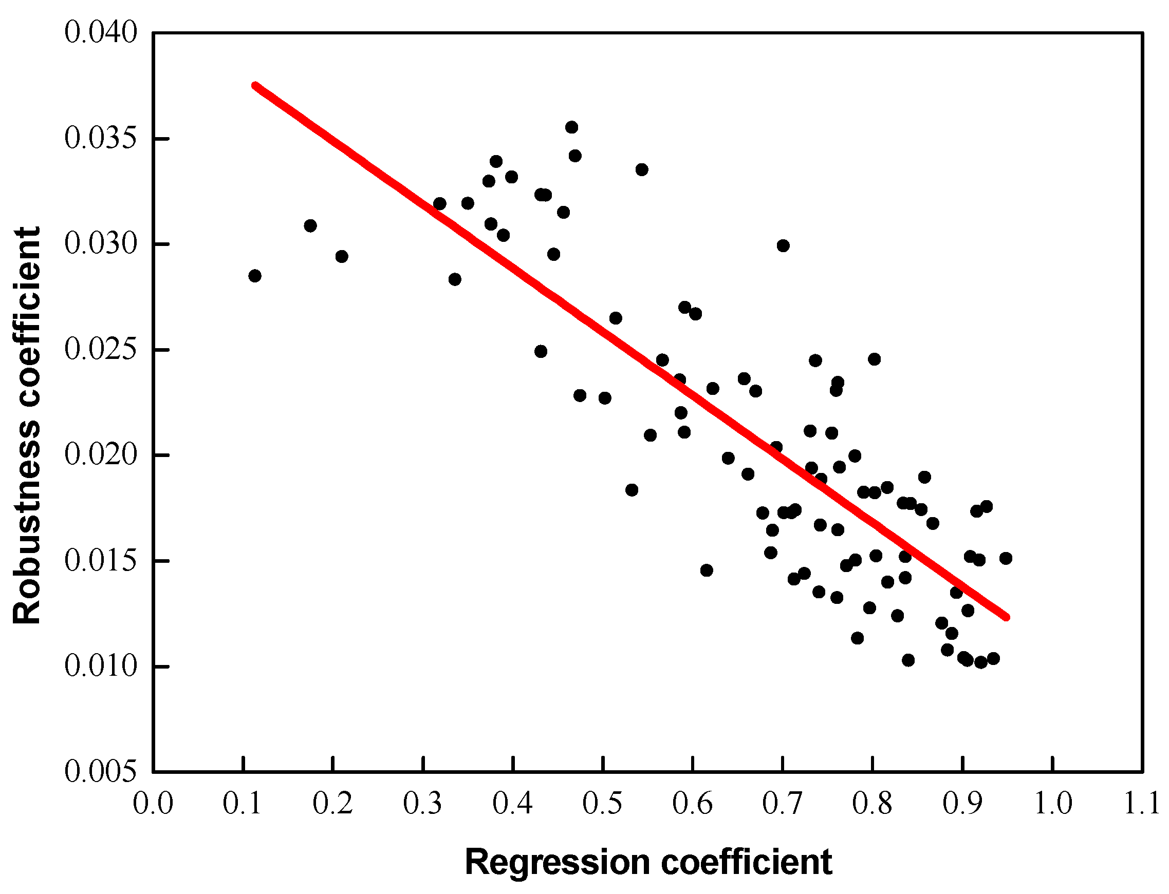
3.2. Analysis of Robustness to Noisy Data

System parameter uncertainty is often inevitable in practice. Inaccurate measurements may cause the parameters’ tested values to deviate from their true values. Robustness is a measure of a system’s ability to maintain its expected performance under some kind of disturbance, including model inaccuracy [24]. Due to the limited sensitivity and resolution of the measurements, the training data including internal resistance and capacity measurement may be different from the true value:

$$R_i^{\text{m}}=R_i^{\text{r}}+{\text{γ}}_{\text{e}}$$

(5)

where $R_i^{\text{m}}$ is the measured value; $R_i^{\text{r}}$ is the true value of the internal resistance; and γ_e is a random testing error. Ideally γ_e = 0 and $R_i^{\text{m}}=R_i^{\text{r}}$, thus ANN outputs a true estimate of the capacity $Q_i^{\text{r}}$:

$$Q_i^{\text{r}}={\text{f}}_2({\displaystyle \sum _{j=1}^{S_2}[w_{i,j}^2{Q}_i^{\text{r,1}}+b_i^2]})={\text{f}}_2\left({\displaystyle \sum _{j=1}^{S_2}\left[w_{i,j}^2\left({\text{f}}_1\left\{{\displaystyle \sum _{k=1}^{S_1}{w}_{i,k}^1{R}_i^{\text{r}}+b_i^1}\right\}\right)+b_i^2]\right]}\right)$$

(6)

$$MS{E}_1=\frac{1}{N}{\displaystyle \sum _{i=0}^N{\left(Q_i^{\text{r}}-Q_i^{\text{t}}\right)}^2}$$

(7)

where $w_{i,j}^1$ and $b_i^1$ are the weight and bias from the input layer to the hidden layer, respectively, $w_{i,j}^2$ and $b_i^2$ are the weight and bias from the hidden layer to the output layer, respectively, f(·) represents the transfer function of these layers. The total error function is calculated using the Equation (7). By using the LM gradient algorithm the mean square error of the estimation MSE₁ is reduced and eventually reaches a minimum value MSE_1,min. If however, the measured internal resistance input to the ANN has an error γ_e, then the estimated value of battery capacity and the total error MSE₂ are given by:

$$\begin{array}{l}{Q}_i^{\text{m}}={\text{f}}_2\left\{{\displaystyle \sum _{j=1}^{S_2}\left[w_{i,j}^2{Q}_i^{\text{m},1}+b_i^2\right]}\right\}\\ ={\text{f}}_2\left\{{\displaystyle \sum _{j=1}^{S_2}\left[w_{i,j}^2\left({\text{f}}_1\left({\displaystyle \sum _{k=1}^{S_1}\left[w_{i,k}^1{R}_i^{\text{m}}+b_i^1\right]}\right)\right)+b_i^2\right]}\right\}\\ ={\text{f}}_{\text{2}}\left\{{\displaystyle \sum _{j=1}^{S_2}\left[w_{i,j}^2\left({\text{f}}_1\left({\displaystyle \sum _{j=1}^{S_1}\left[w_{i,j}^1\left(R_i^{\text{r}}+{\text{γ}}_{\text{e}}\right)+b_i^1\right]}\right)\right)+b_i^2\right]}\right\}\end{array}$$

(8)

$$MS{E}_2=\frac{1}{N}{\displaystyle \sum _{i=0}^N{(Q_i^{\text{m}}-Q_i^{\text{t}})}^2}$$

(9)

The error tends to its minimum value MSE_2,min in the training process. After training, the total error in ideal situation MSE_1,min and the total error in practical situation MSE_2,min have a deviation ∆MSE, which is an estimation error resulting from measurement error of the neural network model’s input, the internal resistance:

$$\Delta MSE=\left|MS{E}_{1,\min }-MS{E}_{2,\min }\right|$$

(10)

A random error γ_e is used to imitate the estimation error ∆MSE; this random error is also called accidental error or ambiguity error. Random errors occur due to a series of small random fluctuations of the relevant factors during the test. Its characteristics can be summarized as follows: amplitudes and directions are indeterminate, immeasurable and unable to calibrate and the average of the error tends to be zero over time.

The robustness of the BP ANN is examined by adding white Gaussian noise to the tested internal resistance to imitate random errors during the measurement process. Random numbers with Gaussian distribution are produced, with an average value E(γ_e) = 0. The variance can be calculated as:

$${\text{σ}}^2=E({\text{γ}}_{\text{e}}^2)=E({(R_i^{\text{m}}-{\overline{R}}_i^{\text{m}})}^2)$$

(11)

A variance of σ² = 0.02 is set. Assignment of the initial weights of the neural network model is done randomly and BP networks with different weights can be established. The regression coefficient is taken as an indicator of ANN’s precision; the bigger the coefficient the higher accuracy the model will be. To assess the ANN’s robustness, a robustness coefficient is defined as the reciprocal of output (capacity) error variance:

$$\text{λ}=\frac{1}{{\text{σ}}_{\Delta Q_i}^2}=\frac{1}{{\text{σ}}_{(Q_i^{\text{t}}-Q_i^{\text{e}})}^2}=\frac{1}{E({(Q_i^{\text{e}}-Q_i^{\text{t}})}^2)}$$

(12)

The bigger the coefficient, the better the ANN’s robustness is. One hundred times training with different weights was executed, respectively, and the relationship between the robustness coefficient and regression coefficient of the model is illustrated in Figure 10. Correlation between the two is inspected by using Pearson related coefficient, which is given by:

$$\text{ρ}=\frac{\text{COV}(\text{ε,λ})}{\sqrt{D(\text{ε})}\sqrt{D(\text{λ})}}$$

(13)

Where COV represents the covariance of ε and λ. The Pearson related coefficient is found to be −0.805, which indicates that they have a significant negative correlation and the robustness coefficient is a decreasing function of the regression coefficient, i.e., the robustness coefficient decreases with the increase of the regression coefficient.

Figure 10. Relationship between the model regression coefficient and robustness coefficient.

Figure 10. Relationship between the model regression coefficient and robustness coefficient.

Employing the ANN established in Section 3, with a regression coefficient of 0.968, the output capacity estimated value with white noise added to the internal resistance input is illustrated in Figure 11. It can be seen that after adding the white noise to the input, the difference of the estimated and the true values increases significantly compared to Figure 7. The robustness coefficient of the model with high estimation accuracy significantly decreases. The scatter of the estimated capacity also increases significantly. The absolute estimation error statistics are illustrated in Figure 12. The maximum absolute error reaches 44 A·h, and the estimation values are reduced overall.

Figure 11. Estimated and true capacities when white noise is added to the measured internal resistance using an ANN with a regression coefficient of 0.968.

Figure 11. Estimated and true capacities when white noise is added to the measured internal resistance using an ANN with a regression coefficient of 0.968.

Figure 12. Statistical characters of absolute errors (∆e) between ANN model outputs and true value when white noise is added to the input of an ANN with a regression coefficient of 0.968.

Figure 12. Statistical characters of absolute errors (∆e) between ANN model outputs and true value when white noise is added to the input of an ANN with a regression coefficient of 0.968.

The reason for the above results is as follows: when an ANN model is highly accurate, it remembers not only the sample’s general features, but also individual characteristics (such as random noise), and thus it doesn’t have tolerance to faults in the input internal resistance acquisition.

In the remainder of this paper, a method that can balance an ANN model accuracy and robustness is developed. The model can not only satisfy the accuracy requirements, but also has fault tolerance at the same time. Reducing the accuracy and using 0.75 as the model regression coefficient of the neural network model established in Section 3.1, and inputting the internal resistance with white noise to the ANN model, we got a comparison of the output and the truth of the capacity, as shown in Figure 13, and its statistical characters of absolute errors (∆e) between ANN model outputs and true value is shown in Figure 14. Compared with Figure 11, the scatter of this ANN model’s estimated capacity is obviously smaller than the ANN model with regression coefficient of 0.968, and the maximum estimation error is 15 Ah, and 90% of the cells’ capacity estimation error is within 5%. It indicates that robustness can be improved by lowering the model’s accuracy.

Figure 13. Estimated and true capacities when white noise is added to the measured internal resistance using an ANN with a regression coefficient of 0.75 internal resistance with white noise and the true value.

Figure 13. Estimated and true capacities when white noise is added to the measured internal resistance using an ANN with a regression coefficient of 0.75 internal resistance with white noise and the true value.

Figure 14. Statistical characters of absolute errors (∆e) between ANN model outputs and true value when white noise is added to the input of an ANN with a regression coefficient of 0.75.

Figure 14. Statistical characters of absolute errors (∆e) between ANN model outputs and true value when white noise is added to the input of an ANN with a regression coefficient of 0.75.

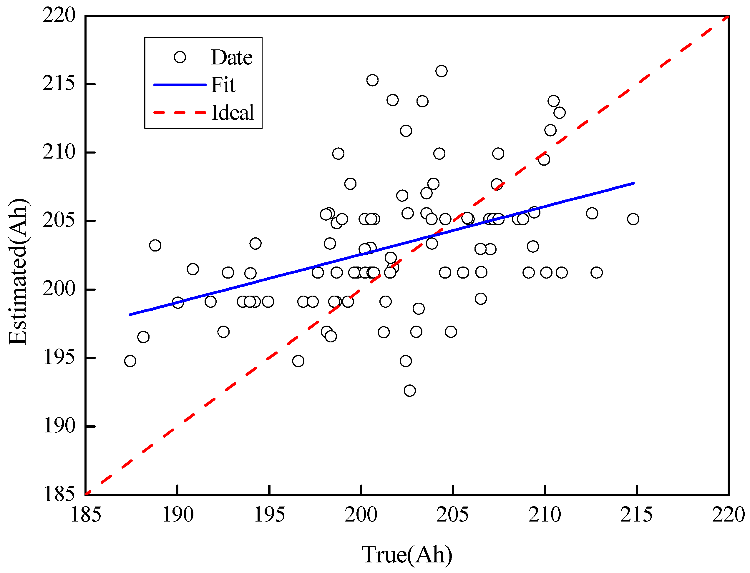
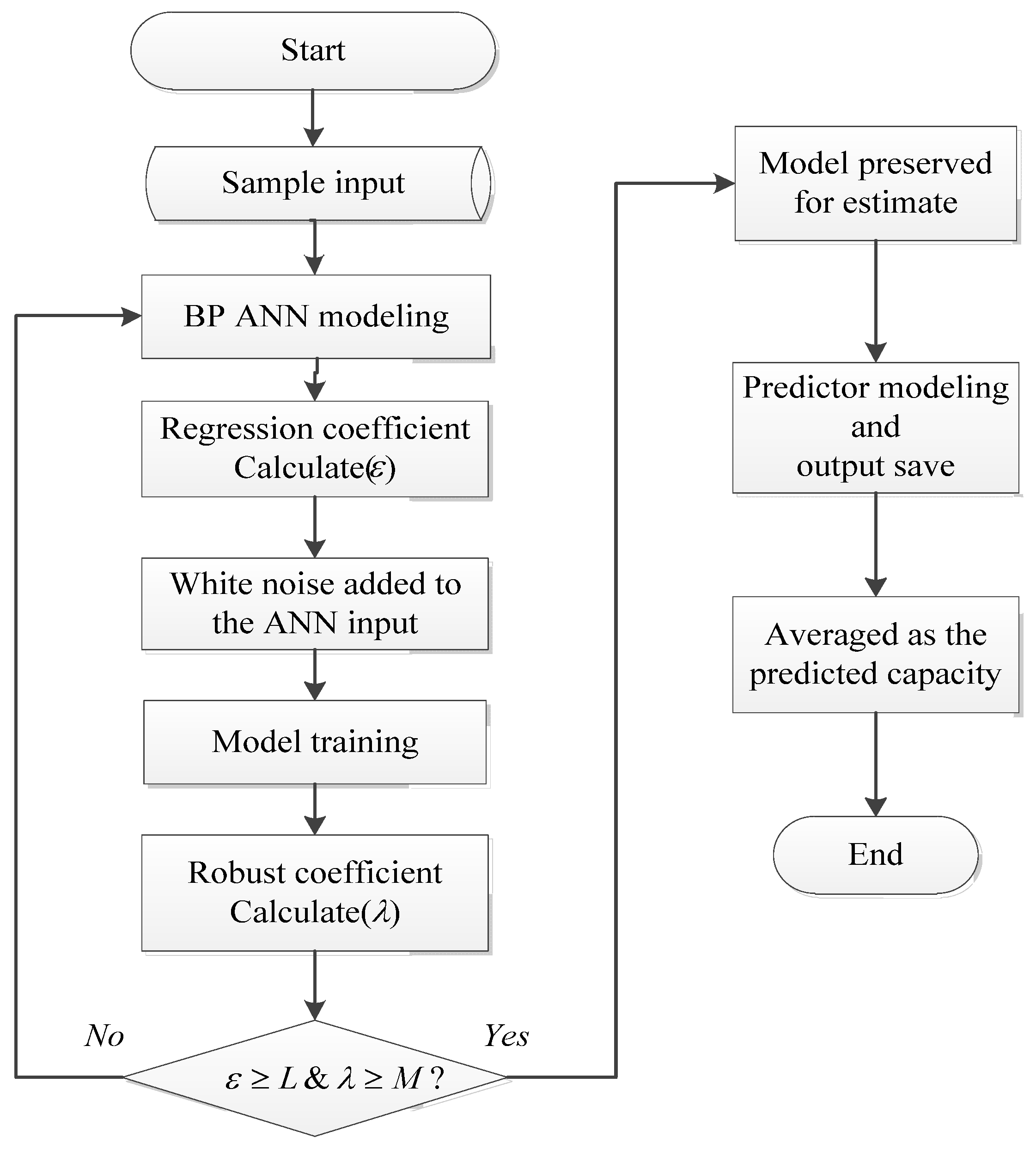
3.3. Proposed Robust Back Propagation Artificial Neural Network

The aforementioned analysis indicates that the robustness coefficient of the BP network model is correlated with the regression coefficient. Reducing the regression coefficient of the model will enhance the robustness of the estimate, but the estimation accuracy will decrease. It is necessary to find a method that optimally balances the relationship between the accuracy and robustness of the ANN capacity estimation model.

The law of large numbers is a theorem expressing the idea that the average of the results obtained from a large number of trials should be approaching the expected value, which is commonly used in noise attenuation and system identification [25,26]. The main idea is that BP ANN modeling is to repeatedly perform in the process of training. The coefficients expressing robustness and regression performance of each model are calculated, respectively. The models will be preserved for capacity prediction if both coefficients are within the set values. The training is stopped till a specified number of models are selected. In the prediction, the chosen weights and neuron biases are then used as the predictor model parameters. The average of the estimated values is regarded as the predictive output:

$$\begin{gathered} z_0=0 \\ {z}_{k+1}=\frac{k}{k+1}{z}_k+\frac{1}{k+1}{Q}_{\text{e},k+1} \\ k=0,1,2,\mathrm{...},N \end{gathered}$$

(14)

$$Q_p=z_N$$

(15)

where Q_e,k+1 represents the (k+1)th network output vector, Q_p is a vector expressing the final predicted output.

The flowchart of the proposed robust BP ANN training method for capacity prediction is illustrated in Figure 15; in which ε and L express the calculated regression coefficient and the threshold, respectively; λ and M represent calculated robustness coefficient and the threshold, respectively. The specific procedure is as follows: first, the internal resistance calculated at for variety of currents at various sampling times, and the measured capacities of the battery in one EV bus were used as training samples to build the BP ANN model. The model regression coefficient was computed to examine its estimation accuracy. Second, white noise was added to the model input, and the robustness coefficient based on Equation (12) was calculated. The ANN model (with specific weighting factors), for which both regression and robustness coefficients meet the requirements, was ultimately chosen to estimate the capacity the battery of another EV bus. Finally, those networks’ capacity estimates outputs were averaged.

The basic principle of robust coefficient selection can be summarized as follows: the regression coefficient is first determined according to model accuracy. Using the specified regression coefficient, a reasonable range of robustness coefficient can be obtained after comparing the model simulation results.

Figure 15. Flowchart of the proposed robust BP ANN training method.

Figure 15. Flowchart of the proposed robust BP ANN training method.

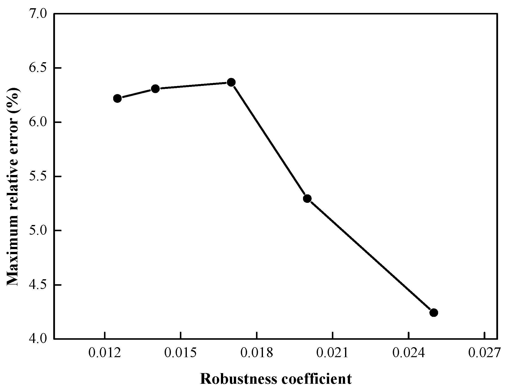
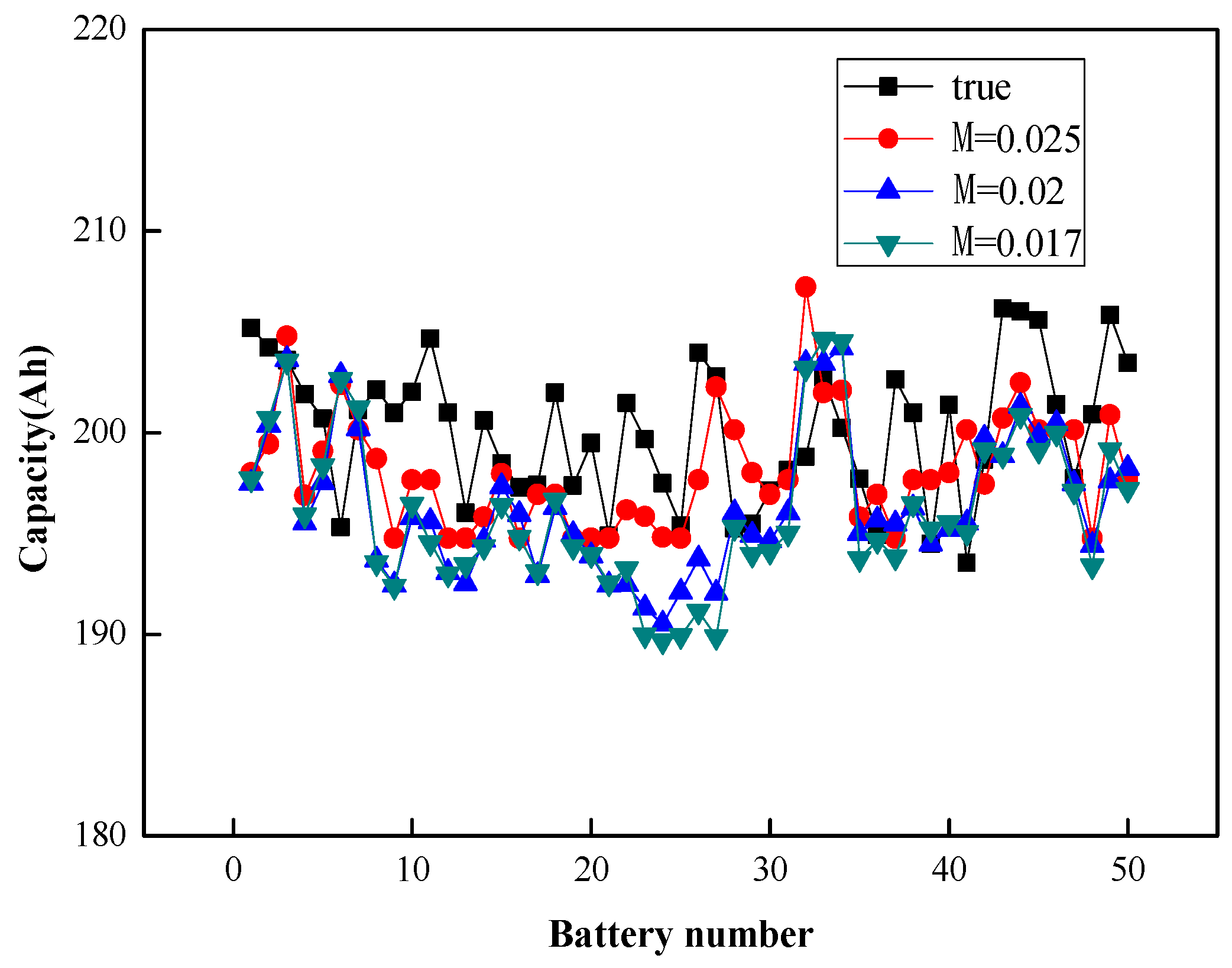
4. Results and Discussion

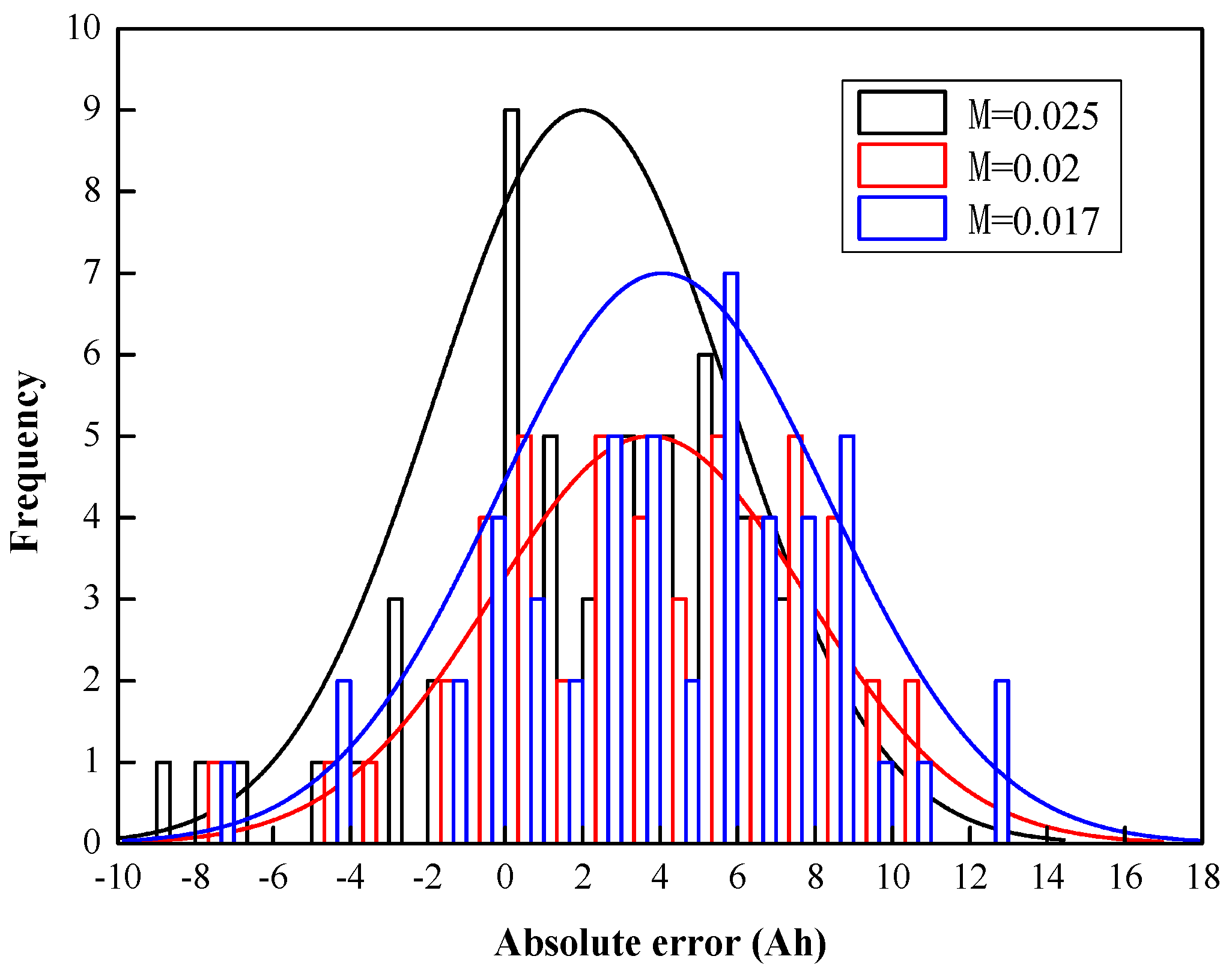
Verification of the proposed robust BP ANN modeling method was performed by testing 50 used EV bus batteries. The threshold value of the regression coefficient is set to 0.65 based on the results. The effect of different threshold values of robustness coefficient on the estimate accuracy was investigated. The maximum relative estimated error as a function of the robustness coefficient is illustrated in Figure 16. The maximum relative estimate errors remain approximately constant when the limit value of the robustness coefficient M ranges from 0.0125 to 0.017, suggesting that the fault tolerance capability of the model is poor in this range. The estimation error decreases significantly when 0.017 ≤ M ≤ 0.025, which indicates that the fault tolerance of the ANN model can improve the estimation accuracy in this range. M is rarely greater than 0.025. It is therefore concluded that a reasonable range of the liminal value of the robustness coefficient is [0.017, 0.025] at the specified limits of the regression coefficient. The true and the predicted capacity for different liminal values of the robust coefficient are shown in Figure 17, and the statistical characteristics of the prediction error are illustrated in Figure 18.

From Figure 17 and Figure 18, it is clear that the difference between the predicted value and true value decrease as the robustness coefficient increases in the specified range and the error of the mean gets closer to zero. A comparison of the predicted results for different robustness coefficients is shown in Table 1. It is suggested that the maximum prediction error is 6.8%, and 94% of the battery samples’ prediction error is controlled within 5% when M = 0.017. The maximum prediction error when M = 0.02 decreases by 1.21% compared to M = 0.017, and 96% of the samples’ prediction error is within 5%. All the battery samples’ prediction error can be controlled within 5% when M = 0.025, and the average error reduces to 1.8%.

Figure 16. The maximum relative estimate error as a function of the robustness coefficient.

Figure 16. The maximum relative estimate error as a function of the robustness coefficient.

Figure 17. The measured capacity and the predicted capacity for different liminal values of the robust coefficient.

Figure 17. The measured capacity and the predicted capacity for different liminal values of the robust coefficient.

Figure 18. The statistical characters of the prediction error for different liminal values of robustness coefficient.

Figure 18. The statistical characters of the prediction error for different liminal values of robustness coefficient.

Table 1. Comparison of predicted results for different robustness coefficients.

Liminal value of robustness coefficient	Maximum absolute prediction error (A·h)	Maximum relative prediction error (%)	Absolute average error (A·h)	Relative average error (%)	The Percentage of relative error less than 5%	MSE
M = 0.017	12.911	6.367	4.891	2.431	94	34.386
M = 0.02	10.736	5.294	4.593	2.282	96	30.146
M = 0.025	8.431	4.241	3.598	1.792	100	18.300
M = 0.03	NA	NA	NA	NA	NA	NA

Table 1. Comparison of predicted results for different robustness coefficients.

Liminal value of robustness coefficient	Maximum absolute prediction error (A·h)	Maximum relative prediction error (%)	Absolute average error (A·h)	Relative average error (%)	The Percentage of relative error less than 5%	MSE
M = 0.017	12.911	6.367	4.891	2.431	94	34.386
M = 0.02	10.736	5.294	4.593	2.282	96	30.146
M = 0.025	8.431	4.241	3.598	1.792	100	18.300
M = 0.03	NA	NA	NA	NA	NA	NA

None of the models can meet both requirements of L = 0.65 and M = 0.03. The optimal liminal value M = 0.025 of the robustness coefficient is ultimately chosen in this study. It is concluded that improving the robustness coefficient can increase the prediction accuracy over a certain range, and using the laws of large numbers can achieve better capacity prediction of the battery status. The simulation results demonstrated the efficacy of the proposed modeling method.

5. Conclusions

Recognizing that measuring the capacity of a large number of used EV batteries is time consuming, and that batteries with the same usage history should exhibit approximately identical statistical characteristics, a BP ANN capacity estimation model with three layers was developed. The internal resistance of the battery, which expresses the kinetics of the battery related to the available capacity, calculated at several sampling times during pulsed current tests is used as the ANN model input. The proposed approach can not only achieve accurate states estimates, but also it is much faster than conventional methods like the full charge-discharge one.

To optimally balance the relationship between the estimate accuracy and robustness to measurement uncertainty, a robust estimation approach is proposed in the paper. A regression coefficient and a robustness coefficient are introduced to comprehensively evaluate the ANN model’s estimate. The law of large numbers is also employed in calculating the results of the model estimate. The testing data of a battery retired from another EV bus was used to verify the proposed robust estimation approach. Experimental results demonstrate the efficacy of the BP ANN model with the proposed robust identification approach, providing foundations for large scale applications of second-life batteries.

References

1. Mukherjee, N.; Strickland, D.; Cross, A.; Hung, W. Reliability estimation of second life battery system power electronic topologies for grid frequency response applications. In Proceedings of the IET International Conference on Power Electronics, Machines and Drives, Bristol, UK, 27–29 March 2012; pp. 1–6.
2. Keeli, A.; Sharma, R.K. Optimal use of second life battery for peak load management and improving the life of the battery. In Proceedings of the IEEE International Electric Vehicle Conference, Greenville, SC, USA, 4–8 March 2012; pp. 1–6.
3. Neubauer, J.; Pesaran, A. The ability of battery second use strategies to impact plug-in electric vehicle prices and serve utility energy storage applications. J. Power Sources 2011, 196, 10351–10358. [Google Scholar] [CrossRef]
4. Viswanathan, V.V.; Meyer, M.K. Second use of transportation batteries: Maximizing the value of batteries for transportation and grid services. IEEE Trans. Veh. Technol. 2011, 60, 2963–2970. [Google Scholar] [CrossRef]
5. Aylor, J.H.; Thieme, A.; Johnso, B.W. A battery state-of-charge indicator for electric wheelchairs. IEEE Trans. Ind. Electron. 1992, 39, 398–409. [Google Scholar] [CrossRef]
6. Pascoe, P.E.; Anbuky, A.H. A unified discharge voltage characteristic for VRLA battery capacity and reserve time estimation. Energy Convers. Manag. 2004, 45, 277–302. [Google Scholar] [CrossRef]
7. Huet, F. A review of impedance measurements for determination of the SOC or state of health of secondary batteries. J. Power Sources 1998, 70, 59–69. [Google Scholar] [CrossRef]
8. Lee, S.; Kim, J.; Lee, J.; Cho, B.H. State-of-charge and capacity estimation of lithium-ion battery using a new open-circuit voltage versus state-of-charge. J. Power Sources 2008, 185, 1367–1373. [Google Scholar] [CrossRef]
9. Xiong, R.; Sun, F.; Chen, Z.; He, H. A data-driven multi-scale extended Kalman filtering based parameter and state estimation approach of lithium-ion polymer battery in electric vehicles. Appl. Energy 2014, 113, 463–476. [Google Scholar] [CrossRef]
10. Kim, J.; Lee, S.; Cho, B.H. Complementary cooperation algorithm based on DEKF combined with pattern recognition for SOC/capacity estimation and SOH prediction. IEEE Trans. Power Electron. 2012, 27, 436–451. [Google Scholar] [CrossRef]
11. Xiong, R.; He, H.; Sun, F.; Zhao, K. Evaluation on state of charge estimation of batteries with adaptive extended Kalman filter by experiment approach. IEEE Trans. Veh. Technol. 2013, 62, 108–117. [Google Scholar] [CrossRef]
12. Klass, V.; Behm, M.; Lindbergh, M. A support vector machine-based state-of-health estimation method for lithium-ion batteries under electric vehicle operation. J. Power Sources 2014, 270, 262–272. [Google Scholar] [CrossRef]
13. Weigert, T.; Tian, Q.; Lian, K. State-of-charge prediction of batteries and battery-supercapacitor hybrids using artificial neural networks. J. Power Sources 2011, 196, 4061–4066. [Google Scholar] [CrossRef]
14. Eddahech, A.; Brlat, O.; Vinassa, J.M. Adaptive voltage estimation for EV li-ion cell based on artificial neural networks state-of-charge meter. In Proceedings of the IEEE International Symposium on Industrial Electronics (ISIE), Hangzhou, Zhejiang, China, 28–31 May 2012; pp. 1318–1324.
15. Yan, Z.; Wang, J. Model predictive control of nonlinear systems with unmodeled dynamics based on feedforward and recurrent neural networks. IEEE Trans. Ind. Inform. 2012, 8, 746–756. [Google Scholar] [CrossRef]
16. Dai, S.L.; Wang, C.; Luo, F. Identification and learning control of ocean surface ship using neural networks. IEEE Trans. Ind. Inform. 2012, 8, 801–810. [Google Scholar] [CrossRef]
17. Lin, H.T.; Liang, T.J.; Chen, S.M. Estimation of battery state of health using probabilistic neural network. IEEE Trans. Ind. Inform. 2013, 9, 679–685. [Google Scholar] [CrossRef]
18. Shen, Y. Adaptive online state-of-charge determination based on neuro-controller and neural network. J. Power Sources 2010, 51, 1093–1098. [Google Scholar]
19. Xia, C.; Guo, C.; Shi, T. A Neural-network-identifier and fuzzy-controller-based algorithm for dynamic decoupling control of permanent-magnet spherical motor. IEEE Trans. Ind. Electron. 2010, 57, 2868–2878. [Google Scholar] [CrossRef]
20. Eddahech, A.; Briat, O.; Bertrand, N.; Delétage, J.Y.; Vinassa, J.-M. Behavior and state-of-health monitoring of Li-ion batteries using impedance spectroscopy and recurrent neural networks. Int. J. Electr. Power Energy Syst. 2012, 42, 487–494. [Google Scholar] [CrossRef]
21. Mingant, R.; Bernard, J.; Moynot, V.S.; Delaille, A.; Mailley, S.; Hognon, J.-L.; Huet, F. EIS measurements for determining the SOC and SOH of Li-ion batteries. ECS Trans. 2011, 33, 41–53. [Google Scholar]
22. Wilamowski, B.M. Neural network architectures and learning algorithms. IEEE Mag. Ind. Electron. 2009, 3, 56–63. [Google Scholar] [CrossRef]
23. Zhang, C.P.; Zhang, C.N.; Liu, J.Z.; Sharkh, S.M. Identification of dynamic model parameters for lithium-ion batteries used in hybrid electric vehicles. High Technol. Lett. 2009, 16, 6–12. [Google Scholar] [CrossRef]
24. Guo, L.D.; Gu, H.; Zhang, D.Q. Robust stability criteria for uncertain neutral system with interval time varying discrete delay. Asian J. Control. 2010, 12, 739–745. [Google Scholar]
25. Liu, L.Z.; Wang, L.Y.; Chen, Z.Q.; Wang, C.S.; Lin, F.; Wang, H.B. Integrated system identification and state-of-charge estimation of battery systems. IEEE Trans. Energy Convers. 2013, 28, 12–23. [Google Scholar] [CrossRef]
26. Ljung, L. System Identification: Theory for the User, 2nd ed.; Prentice-Hall: Englewood Cliffs, NJ, USA, 1999. [Google Scholar]