A Novel Quantum-Behaved Lightning Search Algorithm Approach to Improve the Fuzzy Logic Speed Controller for an Induction Motor Drive

Abstract

This paper presents a novel lightning search algorithm (LSA) using quantum mechanics theories to generate a quantum-inspired LSA (QLSA). The QLSA improves the searching of each step leader to obtain the best position for a projectile. To evaluate the reliability and efficiency of the proposed algorithm, the QLSA is tested using eighteen benchmark functions with various characteristics. The QLSA is applied to improve the design of the fuzzy logic controller (FLC) for controlling the speed response of the induction motor drive. The proposed algorithm avoids the exhaustive conventional trial-and-error procedure for obtaining membership functions (MFs). The generated adaptive input and output MFs are implemented in the fuzzy speed controller design to formulate the objective functions. Mean absolute error (MAE) of the rotor speed is the objective function of optimization controller. An optimal QLSA-based FLC (QLSAF) optimization controller is employed to tune and minimize the MAE, thereby improving the performance of the induction motor with the change in speed and mechanical load. To validate the performance of the developed controller, the results obtained with the QLSAF are compared to the results obtained with LSA, the backtracking search algorithm (BSA), the gravitational search algorithm (GSA), the particle swarm optimization (PSO) and the proportional integral derivative controllers (PID), respectively. Results show that the QLASF outperforms the other control methods in all of the tested cases in terms of damping capability and transient response under different mechanical loads and speeds.

1. Introduction

Three-phase induction motors (TIMs) are widely used in numerous applications, such as in factories, the industrial sector, air compressors, fans, railway tractions, pumps, and so on, accounting for approximately 60% of the total industrial electricity consumption [1,2]. A TIM is a dynamic control system that is difficult to represent theoretically; in several applications, the drive systems of TIMs are exposed to sudden changes in speed or mechanical load [3]. For induction motors, the scalar control (i.e., V/f control) method is one of the control techniques most commonly used by researchers because of the low cost and simple structure and design. Moreover, this method can effectively control medium to high speed, and the parameters of induction motors do no need to be considered [1,4]. A voltage source inverter (VSI) is an important part of an electronic device that is used to generate the signals that control voltage and frequency. A VSI depends on the switching control scheme supplied to six insulated-gate bipolar transistors (IGBTs), which are initiated in the inverter, to generate harmonic signals. Various switching control techniques, such as sinusoidal pulse width modulation, space-vector pulse width modulation (SVPWM), carrier-based pulse width modulation, selective harmonic-elimination pulse width modulation and harmonic-band pulse width modulation, have been reported in the literature. SVPWM is utilized to control switching inverters, because it minimizes the switching losses and harmonics of output waveforms [5,6].

Numerous types of speed controllers are available for induction motors. One example is the proportional integral derivative (PID) controller, which is widely utilized in industrial applications because of its simple design and structure. The sensitivity and stability of the controller design are determined by the PID parameters, which include proportional, integral and derivational gains [1]. In [7], a PID controller was used with an indirect field-oriented controller to regulate TIMs. A PID controller controlled the automatic voltage regulator (AVR) in [8]. However, suitable parameters are difficult to obtain for a PID controller, because of its mathematical model transfer functions and trial-and-error considerations [9,10,11].

Controllers based on artificial intelligence have been employed in numerous applications. For example, an artificial neural network (ANN) was used to implement and test the fault identification scheme for a TIM in [12]. An ANN was also employed to estimate the rotor speed in a sensorless vector-controlled induction motor drive in [13]. Adaptive neuro-fuzzy inference systems (ANFIS) are methods within an ANN with a fuzzy logic controller (FLC). In [1], ANFIS was used to regulate the speed control of a TIM. It was also used to adapt the control of a sensorless induction motor in [14]. However, these controllers are hindered by a number of disadvantages, including their huge data requirement, as well as their long learning and training time.

In recent years, techniques that employ FLC have been implemented by numerous researchers in controlling induction motor drives. FLC is easy to implement, and it does not require a mathematical model of the controlled system. FLC has been considered the better alternative compared to other controllers because it can more effectively control speed and mechanical load; as such, FLC exhibits excellent performance in terms of transient reduction and control [11,15,16,17]. FLC is used to select the appropriate timing of intervention for each distribution strategy [15]. In [9], the FLC functioned as the indirect field-oriented controller of a double-star induction machine. An FLC and a sensorless controller were used as vector controllers of an induction motor in [17]. In [18], an FLC and a PI controller were used to create a new control strategy for pitch angle control to improve the power quality and transient stability of a squirrel-cage induction generator. In [10,11,19,20], a PID controller was self-tuned with an FLC to improve its control of an induction motor. However, the process depends on the inputs and outputs of membership functions (MFs), which pertain to the number of rules and rule bases. These variables are determined by a trial-and-error procedure, which is time consuming [11,16].

Recently, optimization techniques have been employed to design the speed controller of an induction motor. Optimization techniques include the genetic algorithm (GA) and particle swarm optimization (PSO), among others. In [1,21], GA was used to select PID coefficients to control the speed of an induction motor. PSO improved the PID controller of an AVR in [8]. In [16], a differential search algorithm was used in FLC design optimization techniques to develop an FLC for photovoltaic inverters. In [22], an optimal FLC-based maximum power point tracking algorithm for photovoltaic systems is presented to improve FLC with the use of the PSO algorithm. In [23], a GA was used to enhance the fuzzy-phase plane controller for the optimal position/speed tracking control of an induction motor. The GA–PSO algorithm was applied to improve indirect vector control to find the optimal torque control [24]. In [25], PSO was utilized as a model-parameter identification method for permanent magnet synchronous motors.

At present, numerous researchers have shown interest in developing the performance of optimization methods. One of these methods is a quantum system applied to PSO by Sun et al. [26] in 2004. Quantum PSO (QPSO) has been used in several applications, such as in [27,28], because of its powerful performance. In [29,30], QPSO was improved by applying a Gaussian probability distribution; the improved QPSO was used in an economic load dispatch of a power system [31]. In [32], QPSO was used to optimize core fuel management in water-water energy reactor (WWER)-1000. The quantum system was applied to optimize the gravitational search algorithm (GSA) in [33]. In [34], quantum GSA was employed to solve the optimal power-quality monitor-placement problem in power systems. Meanwhile, it was used to solve the thermal-unit commitment problem with wind power integration in [35]. In addition, this algorithm was adopted to address another problem with wind power integration in [36]. In [37], quantum GSA was used to improve classification accuracy with an appropriate feature subset in binary problems. Binary-encoded problems were solved through GSA optimization with quantum computing in [38]. The firefly algorithm was improved using the quantum system. The quantum firefly algorithm was applied to optimize the power-quality monitor placement in a power system in [39]. In [40], the quantum firefly algorithm was used to improve the power quality and reliability of distribution systems.

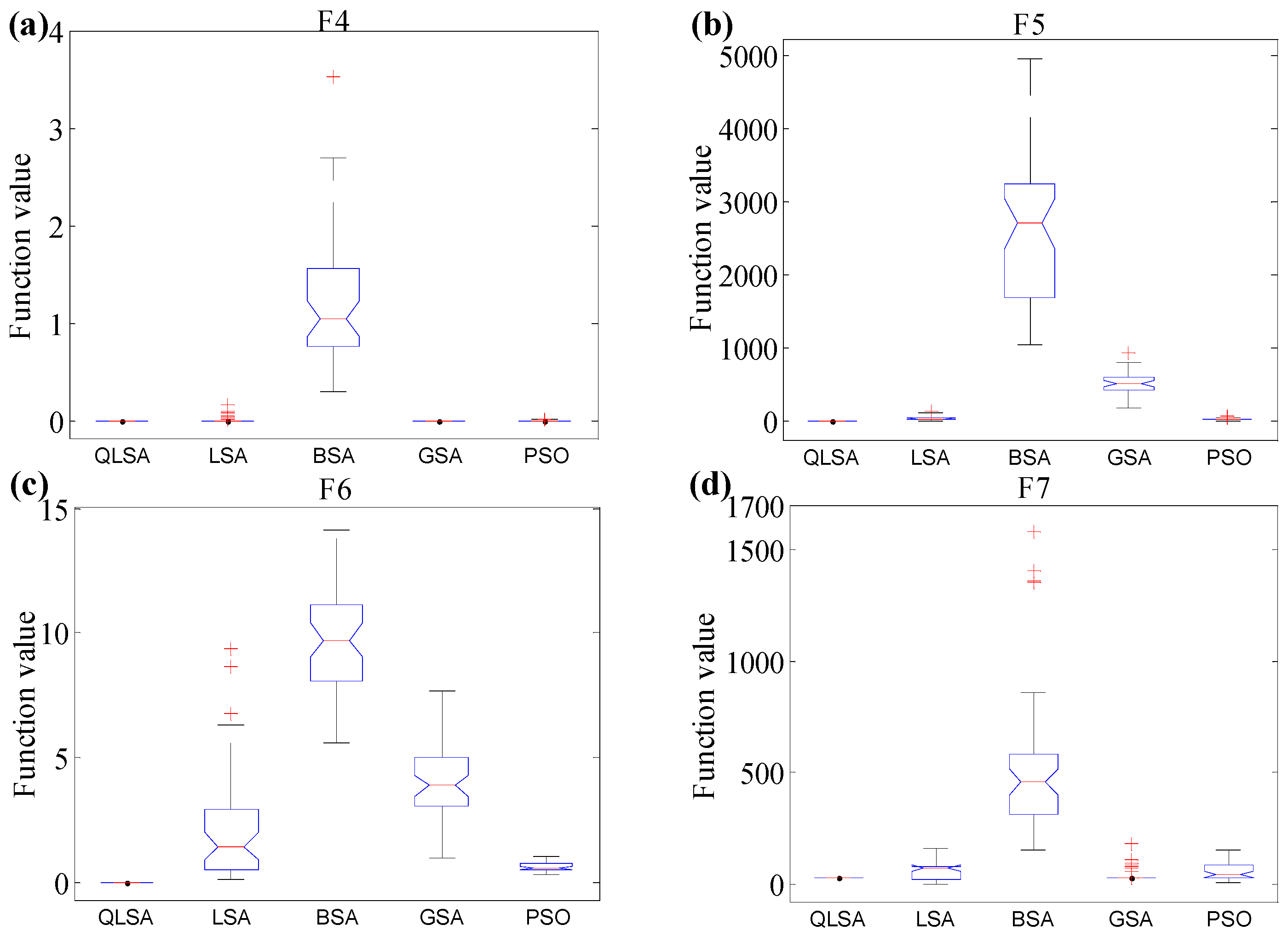
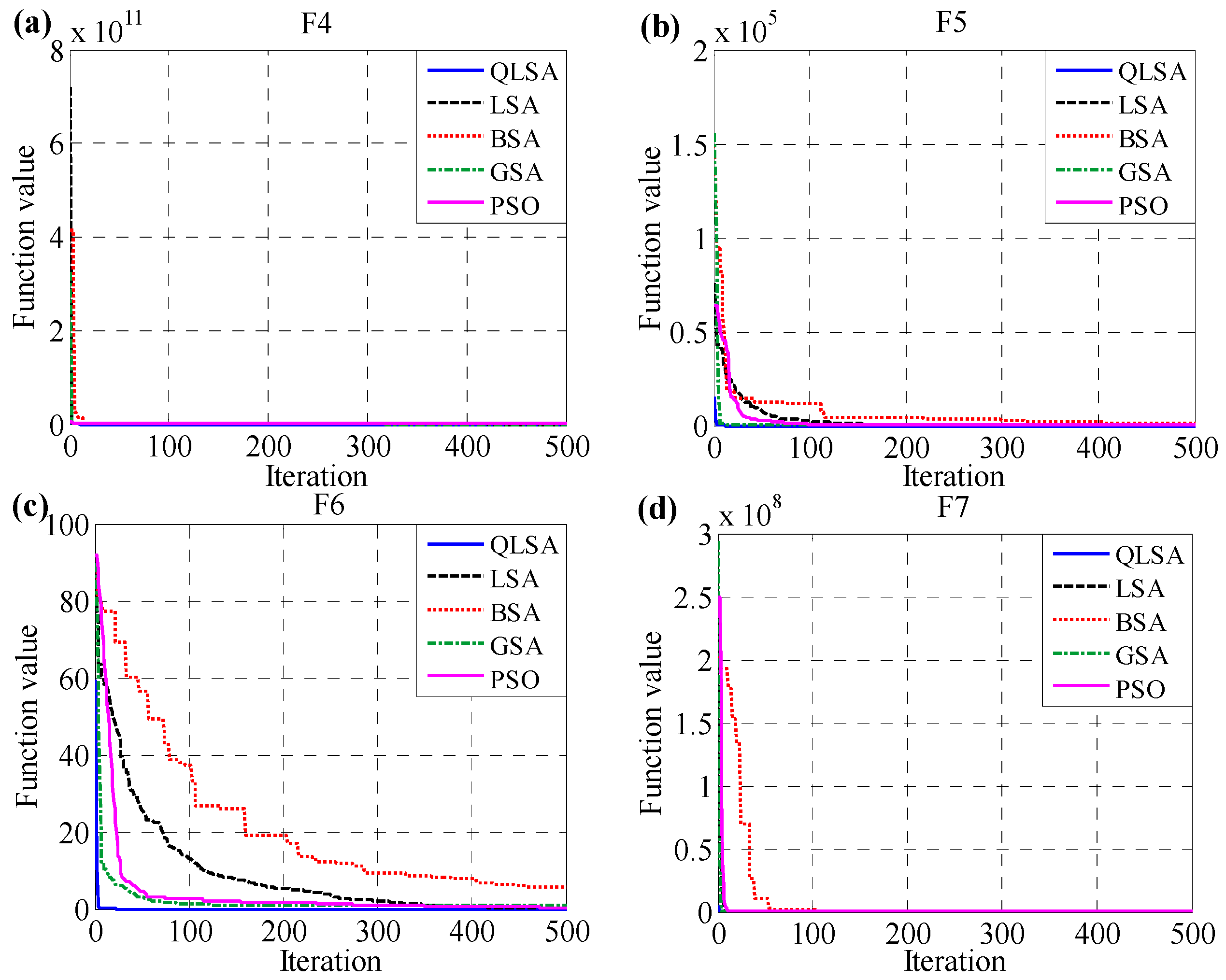
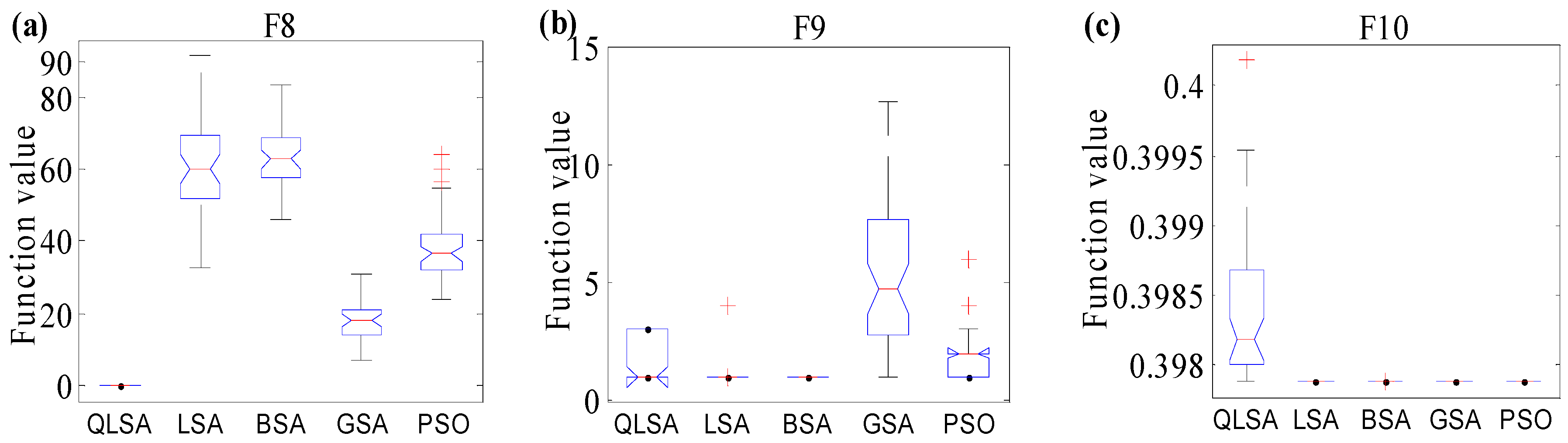
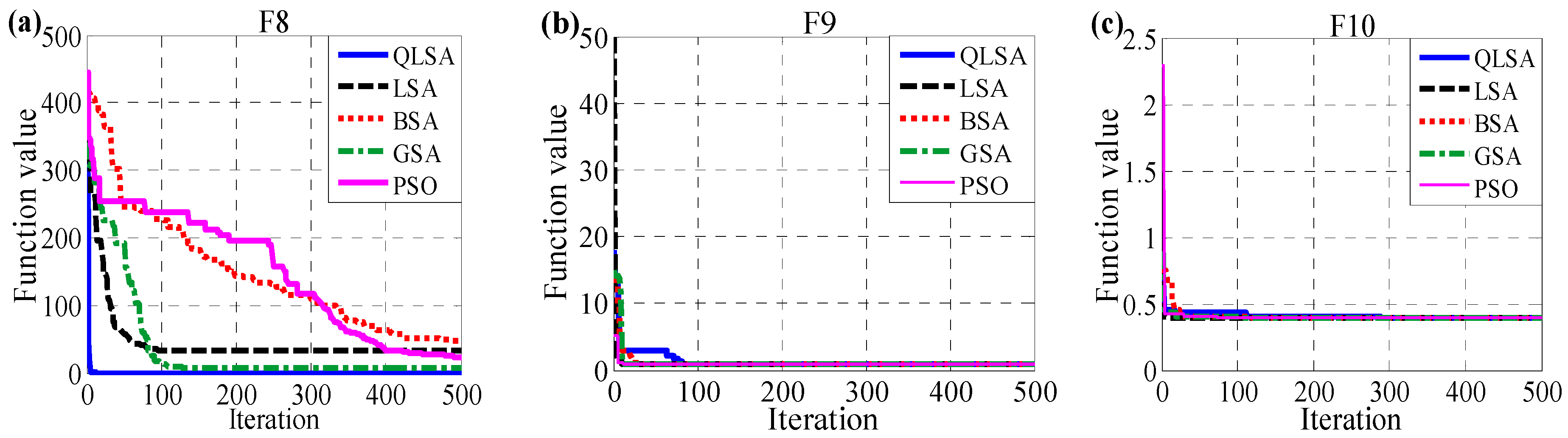
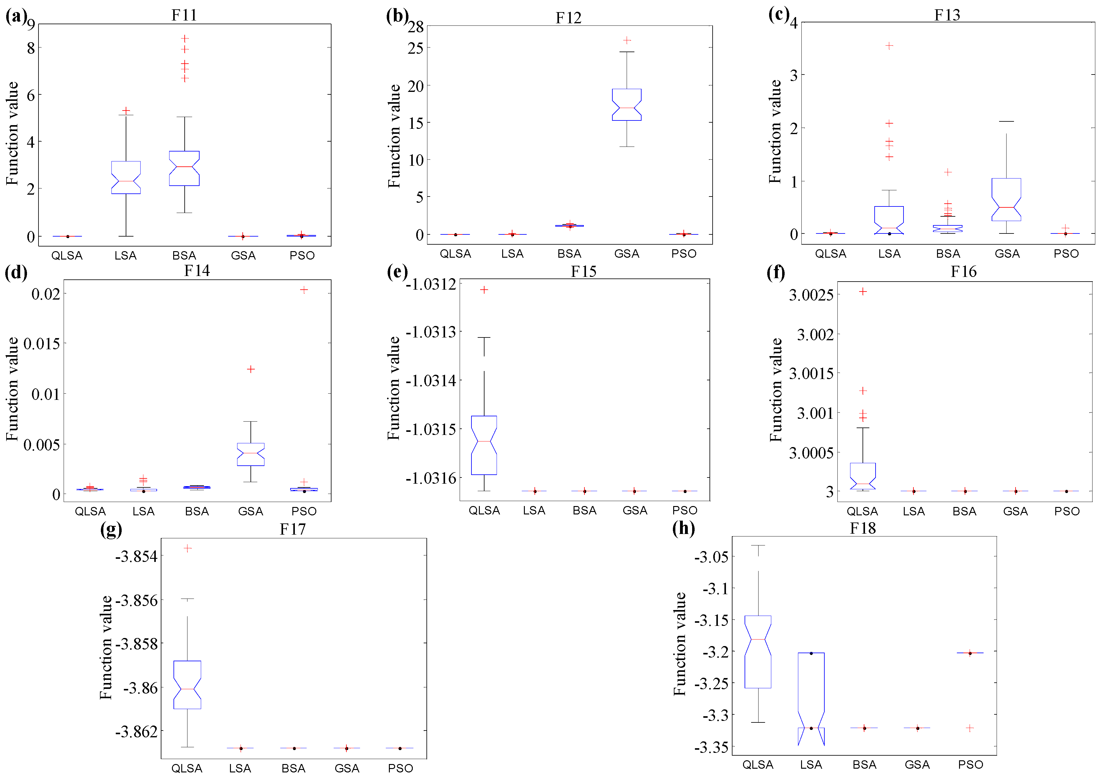
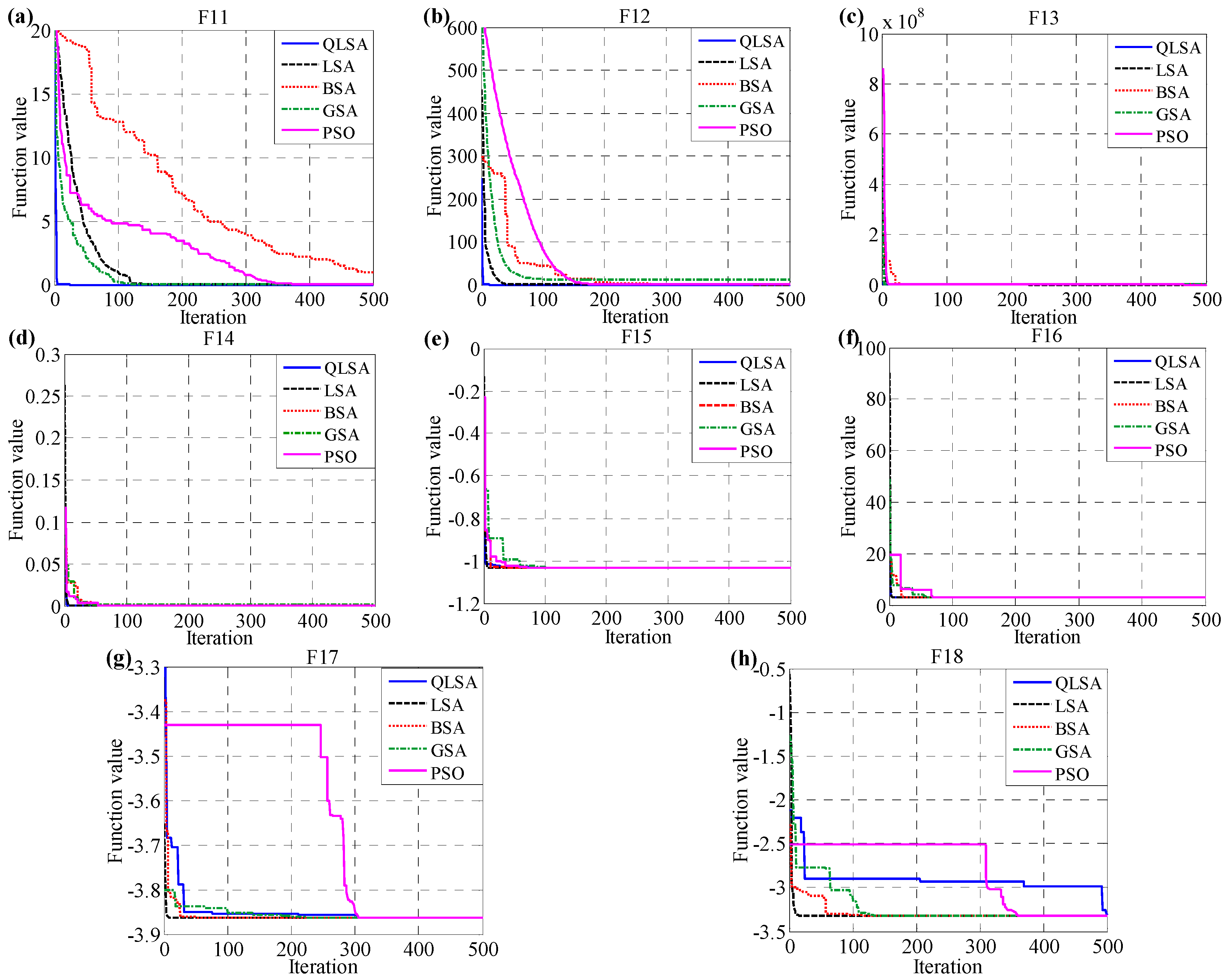
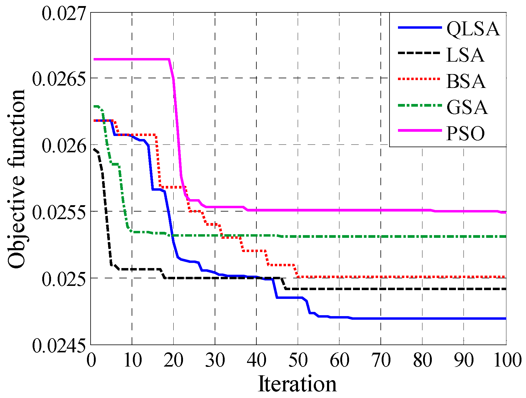
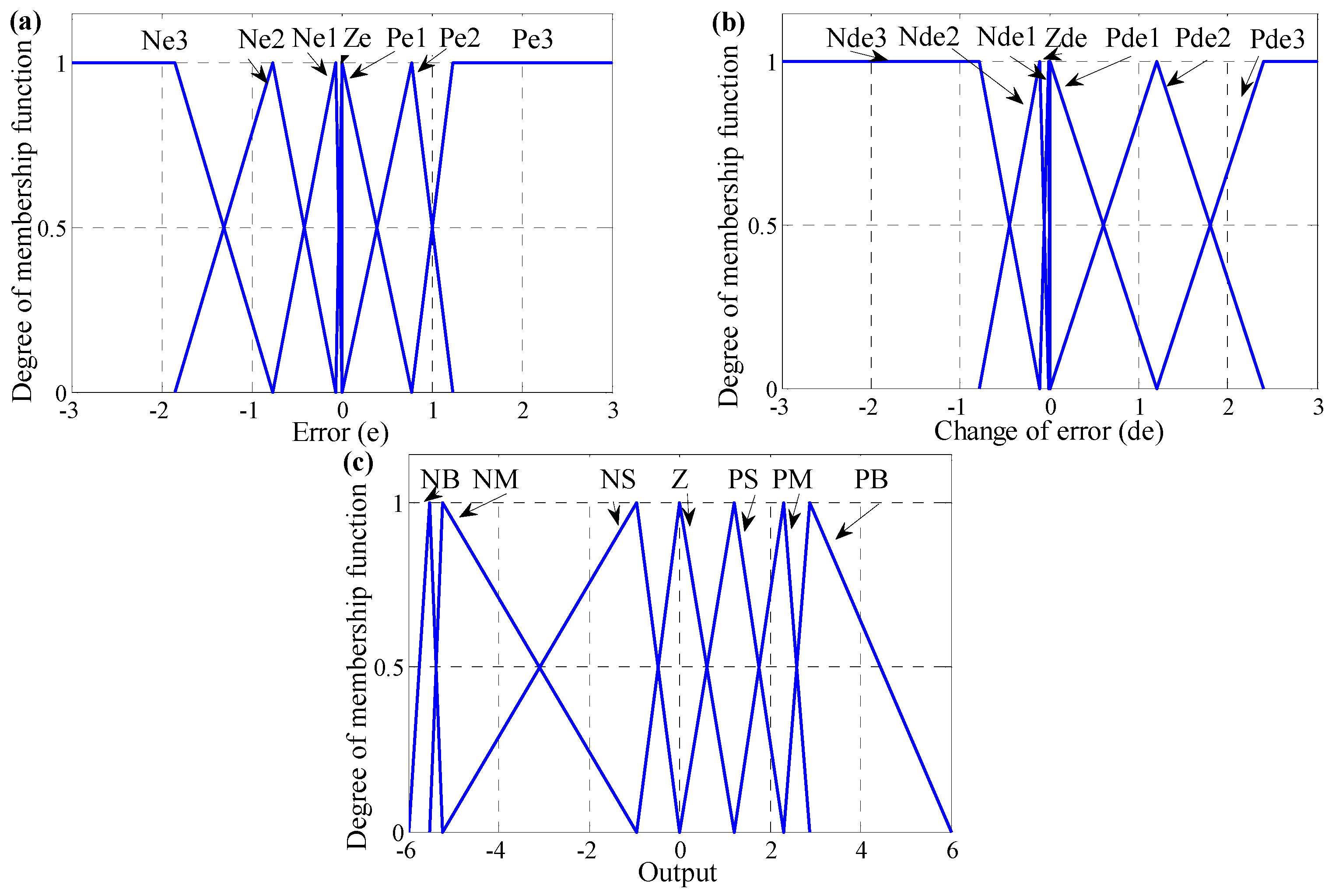
In the present study, a novel optimization method called the quantum-behaved lightning search algorithm (QLSA), is generated to solve constrained optimization problems. This method applies quantum mechanics theories with LSA to enhance the performance of LSA. This work is divided into two experiments. The first experiment comprises an application of 18 benchmark functions and a comparison with four optimization methods, namely the LSA, the backtracking search algorithm (BSA), GSA and PSO, to evaluate the reliability and efficiency of the proposed algorithm. The second experiment is developed to improve the performance of the TIM speed controller by tuning the free parameters and selecting the limits and best values for the input and output of the MFs. The results obtained from the developed QLSA-based FLC (QLSAF) have been compared to the results obtained by other controllers based on LSA, BSA, GSA, PSO and PID under sudden changes in speed and mechanical load. In addition, a high performance of MFs is achieved by minimizing the error function through the use of the mean absolute error (MAE) of the system. Moreover, SVPWM is employed with QLSAF for TIM drives.

2. Quantum-Behaved Lightning Search Algorithm (QLSA)

Numerous optimization methods are available for developing and improving system performance. These methods include GA, simulated annealing, the ant colony search algorithm, PSO, GSA, and so on. In general, optimization techniques are used to solve complex numerical optimization problems, as well as non-linear and non-differentiable systems. In recent years, researchers have focused on developing new optimization techniques that have a significant and powerful role in research development. One of the modern optimization methods is LSA, which was proposed by Shareef et al. [41] in 2015. The mechanism of this method consists of three steps: projectile and step leader propagation, projectile properties and projectile modeling and movement, as explained in [41]. This study is performed based on enhanced LSA using quantum mechanics.

The concept of QLSA involves developing the original LSA by searching for a new position for the population to obtain the best position for step leaders. At the beginning, QLSA is conducted to build memory according to the mean of the best positions of the step leaders, which are called global step leaders$(Gs{l}_{ij}^t)$. Global step leaders represent the best step leaders that can obtain the minimum value of the evaluation. QLSA achieves the attraction and convergence of each step leader with a global minimum and searches for the best position by relying on the stochastic attractor of step leaders $p_j$ as represented in the following novel created equation:

$$p_{ij}^t=\frac{a_{ij}^t.P_{ij,best}^t+b_{ij}^t.Gs{l}_{ij}^t }{c_{ij}^t.F}$$

(1)

for $i=1,2,3,\dots \dots N$, $j=1,2,3,\dots \dots D$ and $t=1,2,3,\dots \dots T$, where $N$, $D$ and $T$ are the population size, the problem dimension and the maximum number of iteration, respectively; a, b and c are three uniformly-distributed random numbers in the range (0,1) for the j-th dimension of step leaders $I$; $P_{ij,\text{best}}^t$ is the best step leader for each population; $Gs{l}_{ij}^t$ is the global step leader for each population; and $F$ is the scale factor, which is suggested to be set between four and 20. This study uses the valu$F=10$.

Suppose that LSA is a quantum system and that each step leader exhibits the quantum behavior with its quantum state formulated by a wave function$\left(\text{ψ}\right)$. ${\left|\text{ψ}\right|}^2$ is the probability density function, which depends on the potential field where the step leader lies. Each individual step leader moves in the search space with a potential on each dimension, of which its center is between points $P_{ij,\text{best}}^{\text{t}}$and$Gs{l}_{ij}^{\text{t}}$. LSA has been considered a step leader in 1D space; a Schrodinger equation solves the time dependency of the 1D potential with point $p$ as the center of potentia $\text{ δ}$. The wave function, at iteration $\left(t+1\right)$, is represented by the following equation [29,30,32]:

$$\text{ψ}\left( P_{ij}^{t+1}\right)=\frac{1}{\sqrt{L_{ij}^t}}\exp (-|P_{ij}^t-p_{ij}^t|/L_{ij}^t)$$

(2)

where $L_{ij}^t$ is the standard deviation of the double exponential distribution, varying with iteration number $t$. Thus, the probability density function $Q$ is a double exponential distribution as follows:

$$Q( P_{ij}^{t+1})={|\text{ψ}( P_{ij}^{t+1})|}^2=\frac{1}{\sqrt{L_{ij}^t}}\exp (-2\left|P_{ij}^t-p_{ij}^t\right|/L_{ij}^t)$$

(3)

In turn, the probability distribution function $M$ is:

$$M( P_{ij}^{t+1})=1-\exp (-2\left|P_{ij}^t-p_{ij}^t\right|/L_{ij}^t)$$

(4)

By using the Monte Carlo method, the j-th component of position $P_i$ at iteration$\left(t+1\right)$can be obtained as follows:

$$P_{ij}^{t+1}=p_{ij}^t\pm \frac{1}{2}{L}_{ij}^t\mathit{ln}(1/u_{ij}^{t+1})$$

(5)

where $u_{ij}^{t+1}$ is a random number uniformly distributed between (0,1). The standard deviation $(L_{ij}^t)$of each step leader is calculated through the equation below:

$$L_{ij}^t=2\text{β}|M{\text{best}}_j^t-P_{ij}^t|$$

(6)

where ${\text{MeanBest}}_j^t$, called the mean best position for step leaders, is defined as the mean value of the ${\text{P}}_{\text{ij},\text{best}}^{\text{t}}$ positions of all step leaders. ${\text{Mbest}}_j^t$ is shown in the equation below:

$${\mathrm{MeanBest}}_j^t=\frac{1}{N}{\displaystyle \sum }_{i=1}^N{P}_{ij}^t=\left(\frac{1}{N}{\displaystyle \sum }_{i=1}^N{P}_{i1}^t,\frac{1}{N}{\displaystyle \sum }_{i=1}^N{P}_{i2}^t,\frac{1}{N}{\displaystyle \sum }_{i=1}^N{P}_{i3}^t, \dots \dots , \frac{1}{N}{\displaystyle \sum }_{i=1}^N{P}_{ij}^t\right)$$

(7)

The contraction expansion coefficient $\left(\text{β}\right)$ works on the tuned contractions to control the convergence speed of the algorithms. The coefficient is calculated as follows:

$$\text{β}={\text{β}}_0+\left(T-t\right)\left({\text{β}}_1-{\text{β}}_0\right)/T$$

(8)

where ${\text{β}}_0$ represents the initial values of the contraction expansion ${\text{ β}}_1$ implies the final values of the contraction expansion, t is the current iteration number and T is the maximum number of iterations. Setting ${\text{β}}_1$ to be larger than 0.8 and smaller than 1.2 is recommended, and ${\text{β}}_0$ should be smaller than 0.6 to generate the acceptable algorithmic performance [29]. $P_{ij}^t$ is the personal best position of step leader $i$. Therefore, the position of the step leaders is updated based on the following equation:

$$P_{ij}^{t+1}=p_{ij}^t\pm \text{β}|{\text{MeanBest}}_j^t-P_{ij}^t|\ln (1/u_{ij}^{t+1})$$

(9)

QLSA has several distinctive properties when compared to the original LSA. First, QLSA explores new positions using an exponential distribution obtained through the global convergence between step leaders; second, QLSA calculates the mean best position to enhance the original LSA; moreover, each step leader in QLSA cannot approach the global best position without regarding other step leaders. The distance between step leaders and ${\text{MeanBest}}_{\text{j}}^{\text{t}}$ directs the new position distribution for each iteration, as shown in Equation (9). Suppose the global best position for a step leader is far from the other step leaders; the ${\text{MeanBest}}_j^t$may be pulled toward the global best position.

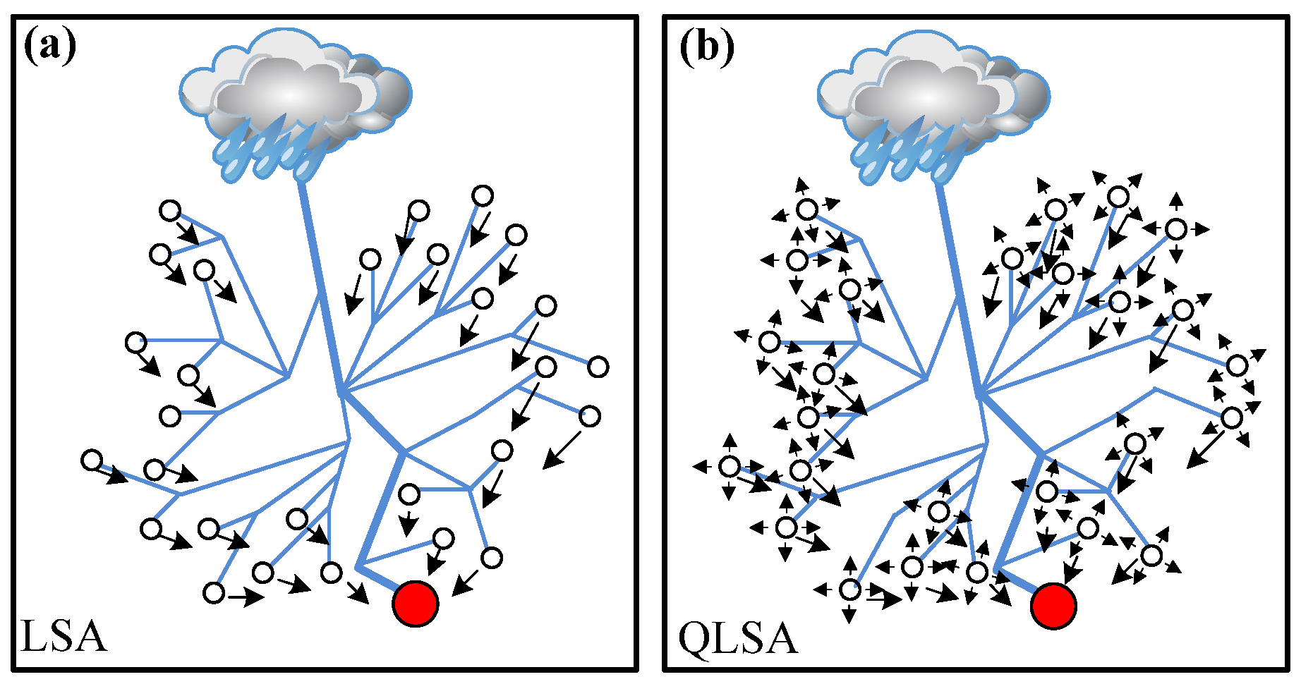
Figure 1 illustrates the spread and relationship between step leaders in the optimization method. The red circle represents the global position for a step leader. The white circles are the other step leaders. The arrows around the small white circles represent the possible directions of the step leaders. In the original LSA, each step leader focuses on the global best position and goes directly to it. The step leaders do not wait or search in space to obtain the new global best position, as presented in Figure 1a. 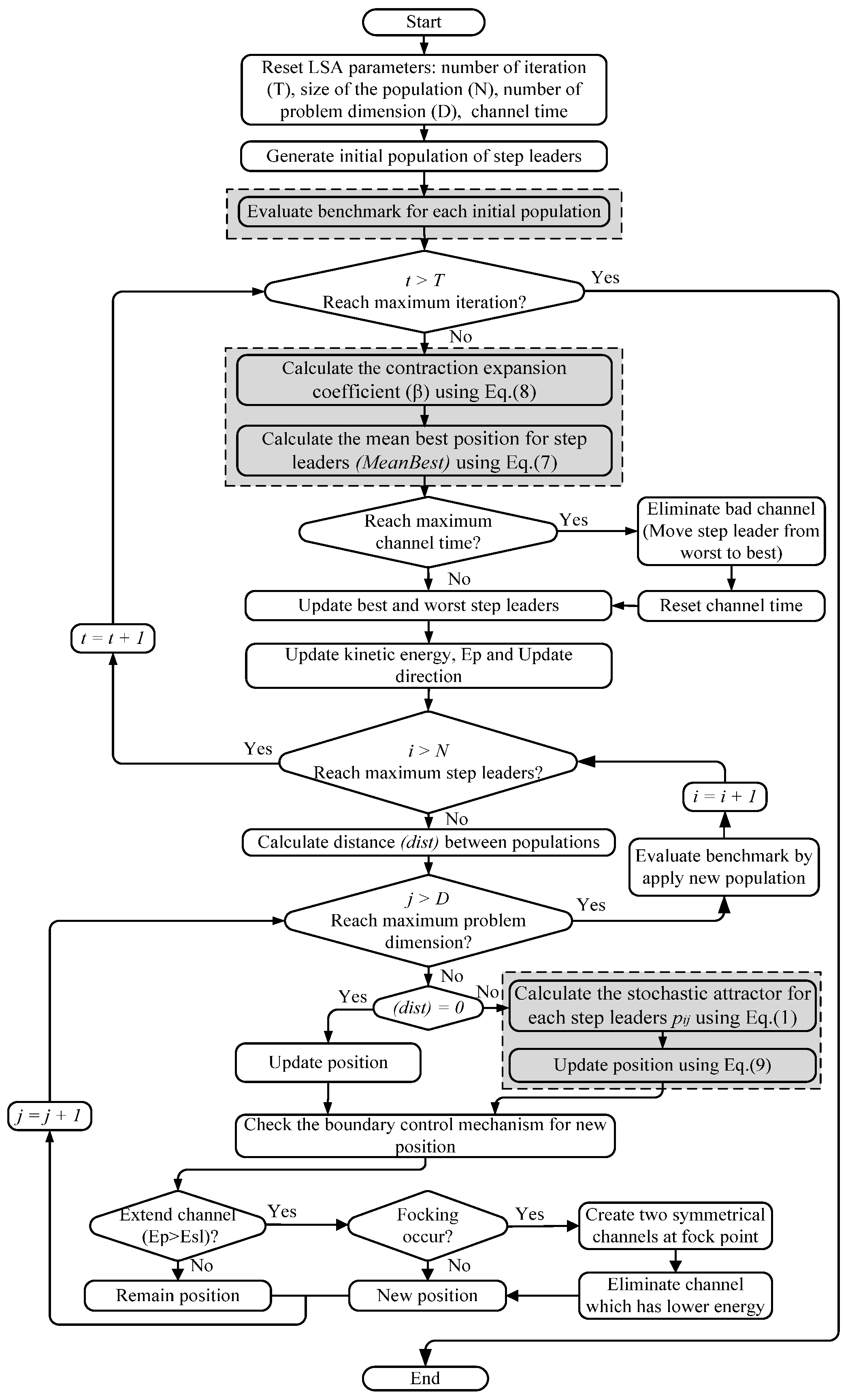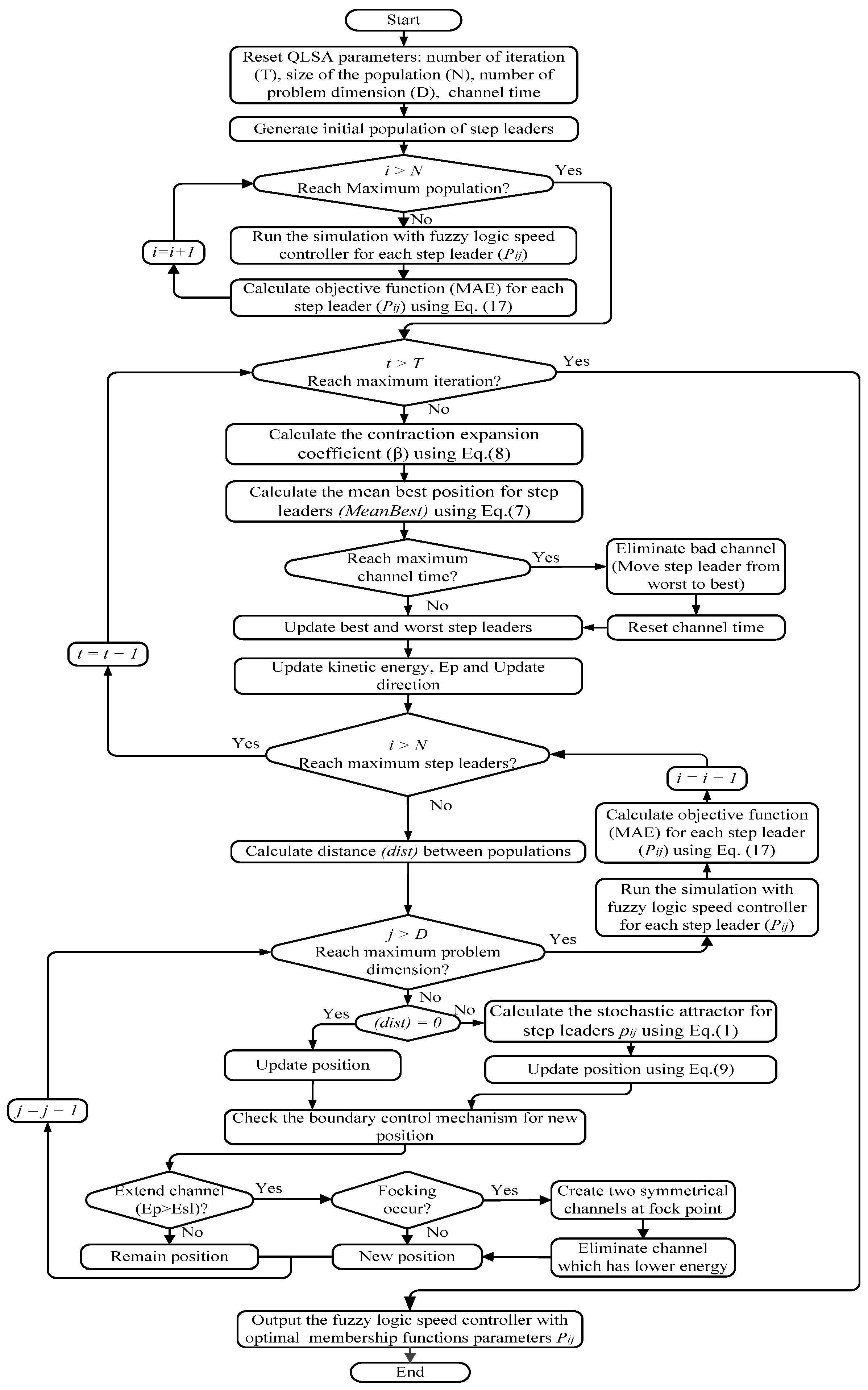By contrast, in QLSA, the step leaders around the global best position may move in any direction to obtain the best new position, as illustrated in Figure 1b. The implementation of QLSA is demonstrated in the flow diagram in Figure 2.

Figure 1. Movements of step leaders in (a) the lightning search algorithm (LSA) and (b) the quantum-behaved LSA (QLSA).

Figure 1. Movements of step leaders in (a) the lightning search algorithm (LSA) and (b) the quantum-behaved LSA (QLSA).

Figure 2. Flow diagram of the proposed QLSA algorithm.

Figure 2. Flow diagram of the proposed QLSA algorithm.

3. QLSA-Based Fuzzy Speed Controller

An FLC is designed to improve speed controller performance in TIM through new optimization techniques. The controller has been trained for all types of sudden changes that occur in a TIM, such as changes in speed and mechanical load. When these changes occur during training, the controller can achieve enhanced performance while operating under a strong control. However, the FLC design must pass through several steps.

3.1. Definition of the Module Properties

The input and output must be selected to determine the fuzzy location, which is a necessary step. The FLC in this study represents the speed controller for a TIM. The input data consist of the error (e) and the change of error (de) for the rotor speed$\left({\text{ω}}_{\text{r}}\right)$, as shown in the equations below. The output controller desired slip speed $\left({\text{ω}}_{\text{sl}}\right)$ is the output variable.

$$e\left(t\right)={\text{ω}}_{\text{r}}^{*}-{\text{ω}}_{\text{r}}\left(t\right)$$

(10)

$$de\left(t\right)=e\left(t\right)-e\left(t-1\right)$$

(11)

3.2. Fuzzification Design

The second step represents the input with a convenient linguistic value by analyzing each input in a group. This step uses a unique MF label, for example “big”, “medium” or “small”. Thus, the FLC depends on the number of MFs used in the linguistic label. The MFs of error and the change of error for the fuzzy speed controller are defined as trapezoidal and triangular MFs. Figure 3a shows that the MFs for error ${\text{μ}}_e\left(e\right)$ consist of three variable$(X_0, X_{1, } X_2)$. Figure 3b shows that the MFs for change of error ${\text{μ}}_{de}\left(de\right)$ consist of three variable$(Z_0, Z_{1 },Z_2)$. The MFs can be represented by the following equations:

$${\text{μ}}_e\left(e\right)=\{\begin{array}{c}\frac{e-X_0}{X_1-X_0} X_0\le e<X_1\\ \frac{e-X_2}{X_1-X_2} X_1\le e<X_2\end{array}$$

(12)

$${\text{μ}}_{de}\left(de\right)=\{\begin{array}{c}\frac{de-Z_0}{Z_1-Z_0} Z_0\le de<Z_1\\ \frac{de-Z_2}{Z_1-Z_2} Z_1\le de<Z_2\end{array}$$

(13)

Figure 3. Triangular representation of membership functions (MFs). (a) Error; (b) change of error.

Figure 3. Triangular representation of membership functions (MFs). (a) Error; (b) change of error.

In a conventional FLC structure, the number of MFs and the boundaries of each MF should be within a suitable range set by the designer through the trial-and-error method until the FLC provides a favorable result. However, this task is difficult to achieve, because identifying the boundaries of MFs is a challenging and time-consuming task.

3.3. Inference Engine Design

The third stage explains how the FLC decides on the TIM based on control rules and linguistic terms. In general, inference systems have two types, namely Mamdani and Takagi–Sugeno. The Mamdani method is used in this study because of its simple structure and design. The fuzzy rule consists of the if-then linguistic term, and the output MFs are operated by the fuzzy rule that is related to both the inputs $\left(e,de\right)$ and the outpu$\left({\text{ω}}_{\text{sl}}\right)$ [11,16,41]. The details of the 49 rules are shown in Table 1 and in the following equations:

Rule 1: If $e$ is “Ne3” and $de$ is “Nde3” THEN ${\mathrm{\omega }}_{sl}$ is “negative big” (NB).

Rule 2: If $e$ is “Ne3” and d$e$ is “Nde2” THEN ${\mathrm{\omega }}_{sl}$ is “NB”.

⋮

Rule 48: If $e$ is “Ne2” and $de$ is “Nde3” THEN ${\mathrm{\omega }}_{sl}$ is “positive big” (PB).

Rule 49: If $e$ is “Ne3” and $de$ is “Nde3” THEN ${\mathrm{\omega }}_{sl}$ is “PB”.

Table 1. Fuzzy rules of the three-phase induction motor (TIM) speed controller.

e		Ne3	Ne2	Ne1	Ze	Pe1	Pe2	Pe3
de	Nde3	NB	NB	NB	NB	NM	NS	Z
	Nde2	NB	NB	NB	NM	NS	Z	PS
	Nde1	NB	NB	NM	NS	Z	PS	PM
	Zde	NB	NM	NS	Z	PS	PM	PB
	Pde1	NM	NS	Z	PS	PM	PB	PB
	Pde2	NS	Z	PS	PM	PB	PB	PB
	Pde3	Z	PS	PM	PB	PB	PB	PB

NB: negative big; NM: negative medium; NS: negative small; Z: zero; PS: positive small; PM: positive medium; PB: positive big.

Table 1. Fuzzy rules of the three-phase induction motor (TIM) speed controller.

e		Ne3	Ne2	Ne1	Ze	Pe1	Pe2	Pe3
de	Nde3	NB	NB	NB	NB	NM	NS	Z
	Nde2	NB	NB	NB	NM	NS	Z	PS
	Nde1	NB	NB	NM	NS	Z	PS	PM
	Zde	NB	NM	NS	Z	PS	PM	PB
	Pde1	NM	NS	Z	PS	PM	PB	PB
	Pde2	NS	Z	PS	PM	PB	PB	PB
	Pde3	Z	PS	PM	PB	PB	PB	PB

NB: negative big; NM: negative medium; NS: negative small; Z: zero; PS: positive small; PM: positive medium; PB: positive big.

3.4. Defuzzification

Defuzzification is the final step in the FLC. This process generates the output values from the controller as crisp values. Moreover, it includes the important part of adjustment and the crisp value control of the output MFs. However, these MFs are required to select the number of MFs and boundaries. Each MF must be suitable to provide the optimized result through the trial-and-error method. In this study, an optimization method is used to find the boundaries of MFs. Several methods are employed to compute the crisp value. The center of gravity approach is considered the best among these methods, as recommended by several authors [22,41].

$$O_{\text{crisp}}=\frac{{{\displaystyle \sum }}_i^n{w}_i.u_i}{{{\displaystyle \sum }}_i^n{w}_i}$$

(14)

where $n$ is the number of rules, $u$ is the value of MFs output and $w$ is the weight coefficient. The weights are calculated through the minimum between ${\text{μ}}_e\left(e\right)$ and ${\text{μ}}_{de}\left(de\right)$, as shown in the following equation:

$$w_i=\min \left[{\text{ μ}}_e\left(e\right),{\text{μ}}_{de}\left(de\right)\right]$$

(15)

3.5. Design of QLSA for the Optimal Fuzzy Logic Speed Controller

The FLC is popular because it is simple, has a low implementation cost and can be applied to non-linear controller systems; this controller does not rely on a mathematical model [7,8]. However, the conventional FLC has a disadvantage in selecting the boundaries of the input and output of MFs [16,41]. This section explains how the improved FLC utilizes QLSA to identify the best boundaries of the input/output of MFs.

The QLSA method for optimal FLC is designed to identify and achieve three basic components, namely input information, objective function and optimization limitations. The input data for the QLSA method of the FLC are the boundary values for the input and output of MFs. The input matrix consists of columns and rows. The number of columns represents the numerical boundary values for error, change of error and output MFs. The number of rows represents the numerical boundary values for population size, as shown in the following matrix:

$$D_{ij}=\left[\begin{array}{ccc}{P}_{11}& \cdots & P_{1j}\\ ⋮& \ddots & ⋮\\ P_{i1}& \cdots & P_{ij}\end{array}\right]$$

(16)

where $D$ is input information to the optimization technique; $i=1,2,\dots \dots ,P$, $P$ is the size of the population; $j=1,2,\dots \dots ,N$, $N$ is the size of problem dimension. Figure 4 presents the 21 problem dimensions included in seven MFs for the error, the change of error and the output. A total of 30 populations is used in this study to obtain the best results.

Figure 4. MFs for: (a) error; (b) change of error; (c) output.

Figure 4. MFs for: (a) error; (b) change of error; (c) output.

QLSA requires an objective function to reduce errors. Therefore, the objective function determines the best value of the FLC output to increase system stability performance. The MAE is used as an objective function to obtain a suitable controller and to improve results. The MAE is calculated as follows:

$$\text{MAE}=\frac{1}{H}{\displaystyle \sum }_{m=1}^H\left|{\text{ω}}_{\text{r}}^{*}-{\text{ω}}_{\text{r}}\right|$$

(17)

where $H$ is the number of samples, ${\text{ω}}_{\text{r}}^{*}$ is the reference rotor speed and ${\text{ω}}_{\text{r}}$ is the rotor speed that is responsible for motor operation. The last basic component is optimization limitations for the FLC. These constraints are important to avoid overlaps between the borders of MFs. Figure 4a shows that the variable $P_{ij}^2$ should not cross the variables $P_{ij}^1$ and $P_{ij}^3$ to avoid an overlap between MFs. Imposing limitations addresses this problem, as shown in the equation below:

$$P_{ij}^{h-1}<P_{ij}^h<P_{ij}^{h+1}$$

(18)

QLSA has been applied to the FLC to select a few important parameters, such as the number of iterations$\left(T\right)$, the number of populations$\left(P\right)$ and the number of problem variables $\left(N\right)$. Figure 5 shows the flow diagram that illustrates the proposed QLSAF.

Figure 5. Proposed QLSA-based optimum fuzzy speed controller design procedure.

Figure 5. Proposed QLSA-based optimum fuzzy speed controller design procedure.

4. QLSA-Based Fuzzy Logic Speed Controller Simulation Model

The developed QLSAF simulation model for a TIM drive model is presented in Figure 6. SVPWM is utilized to control the TIM drive through V/f control and QLSAF. The TIM model is a stationary reference frame in which rotor speed is measured depending on the feedback signal. Therefore, sensor speed must be measured. All possible cases of sudden changes in speed and mechanical load are accomplished in the simulation model to create a powerful TIM controller. The developed controller is also employed to tune the parameters and to determine the best values for the MF parameters through QLSA.

Figure 6 shows that SVPWM receives three input values ($V_{an}$,$V_{bn}\text{ and }{V}_{cn})$ and generates switching signals for the inverter gate drives of the IGBTs to deliver three-phase AC voltages to the TIM. The V/f control strategy is responsible for generating the peak voltage in SVPWM. However, the QLSA-Mamdani fuzzy controller has been used for the speed controller system. This controller allows real speed to track the reference speed. The speed controller provides the required slip speed to reach the reference speed (i.e., synchronous speed). The slip speed is then added to the feedback signal of the rotor speed to achieve the required frequency for the inverter in the TIM. A V/f relationship is essential to fix the machine at its rated flux linkage.

Figure 6. Block diagram of the proposed quantum-behaved lightning search-fuzzy (QLSAF) speed controller for three-phase induction motor (TIM).

Figure 6. Block diagram of the proposed quantum-behaved lightning search-fuzzy (QLSAF) speed controller for three-phase induction motor (TIM).

5. Results and Discussion

Two tests have been conducted in this study. The first test solves specific benchmark optimization problems using QLSA. Eighteen benchmark functions have been used. The second test is a practical application of QLSA to the trial-and-error procedure for obtaining the MFs of the FLC for the induction motors.

5.1. Experiment 1

The proposed method is validated using specific tests. However, the proposed QLSA is applied to a group of 18 benchmark functions. These functions have been employed by several researchers, including Shareef et al. [41], Rashedi et al. [42], Yao [43] and Rao et al. [44], when they developed their optimization algorithms. In particular, the new algorithm is tested and validated through functional characteristics, such as dimensionality, separability and modality. The modality of a function refers to the number of vague peaks in the function surface. A function is multimodal if it has two or more vague peaks. An algorithm that encounters these peaks while searching may be trapped in one of the local minima. Separability indicates the difficulty level of various benchmark functions. In general, separable functions are easier to solve than non-separable functions, because each variable of a function is independent of other variables. Moreover, the difficulty of a problem also increases along with function dimensionality. For highly non-linear problems, dimensionality may be a significant barrier for nearly all optimization algorithms. In this study, 18 benchmark functions are classified according to modality and separability. Four tests are conducted to validate the reliability, strength and efficiency of the proposed QLSA. The proposed QLSA is then compared to four standard optimization methods, namely LSA, BSA, GSA and PSO. To ensure that the comparisons are fair, the population size for all optimization methods is set to 50. The compared optimization methods have several parameter settings, as listed in Table 2.

Table 2. Parameter settings used in quantum-behaved lightning search algorithm (QLSA), lightning search algorithm (LSA), the backtracking search algorithm (BSA), the gravitational search algorithm (GSA) and particle swarm optimization (PSO).

Parameter	QLSA	LSA	BSA	GSA	PSO
Population size	50	50	50	50	50
Maximum iteration	500	500	500	500	500
c1 and c2	-	-	-	-	2
F	-	-	3	-	-
G0 and α	-	-	-	100, 20	-
Channel time	10	10	-	-	-

Table 2. Parameter settings used in quantum-behaved lightning search algorithm (QLSA), lightning search algorithm (LSA), the backtracking search algorithm (BSA), the gravitational search algorithm (GSA) and particle swarm optimization (PSO).

Parameter	QLSA	LSA	BSA	GSA	PSO
Population size	50	50	50	50	50
Maximum iteration	500	500	500	500	500
c1 and c2	-	-	-	-	2
F	-	-	3	-	-
G0 and α	-	-	-	100, 20	-
Channel time	10	10	-	-	-

5.1.1. Test 1

This test determines the reliability, strength and efficiency of QLSA in obtaining the global minimum value when it is applied to benchmark functions with unimodal and separable characteristics. Three benchmark functions are applied in this test. The details are presented in Table 3. This test also compares QLSA with four other methods, namely LSA, BSA, GSA and PSO, for validation. Each benchmark function is tested 50 times. The results that represent the best, worst, median, average and standard deviation of the objective function for each benchmark function are indicated in Table 4. The best result for each benchmark function is written in boldface. The proposed QLSA achieves the best solution for the best global minimum for sphere (Function 1 (F1) and step (F2); for quartic (F3), the proposed method obtains a value near the global minimum. Moreover, the test confirms the powerful performance of QLSA to achieve the best solution in the best, worst, median and standard division values. This result is also observed in the box plot (Figure 7) constructed from the data obtained from the 50 tests. Figure 8 presents the convergence characteristic curves to demonstrate the comparison of the proposed QLSA with the other optimization methods. The QLSA achieves the global minimum faster than the other methods. Thus, the proposed algorithm possesses superior convergence characteristics for this type of function optimization.

Table 3. Unimodal and separable test function.

Function ID	Name	Expression		n	Search Space		Function Minimum
F1	Sphere	$f_1\left(x\right)={\displaystyle \sum _{i=1}^n{x}_i^2}$		30	${\left[-100,100\right]}^n$		0
F2	Step	$f_2\left(x\right)={\displaystyle \sum _{i=1}^n{(\lfloor x_i+0.5\rfloor )}^2}$		30	${\left[-100,100\right]}^n$		0
F3	Quartic	$f_3\left(x\right)={\displaystyle \sum _{i=1}^{n}i{x}_i^4+rand\left(0,1\right)}$		30	${\left[-1.28,1.28\right]}^n$		0

Table 3. Unimodal and separable test function.

Function ID	Name	Expression		n	Search Space		Function Minimum
F1	Sphere	$f_1\left(x\right)={\displaystyle \sum _{i=1}^n{x}_i^2}$		30	${\left[-100,100\right]}^n$		0
F2	Step	$f_2\left(x\right)={\displaystyle \sum _{i=1}^n{(\lfloor x_i+0.5\rfloor )}^2}$		30	${\left[-100,100\right]}^n$		0
F3	Quartic	$f_3\left(x\right)={\displaystyle \sum _{i=1}^{n}i{x}_i^4+rand\left(0,1\right)}$		30	${\left[-1.28,1.28\right]}^n$		0

Figure 7. Variation in global optimization results for benchmark functions in Table 2. (a) F1; (b) F2; (c) F3.

Figure 7. Variation in global optimization results for benchmark functions in Table 2. (a) F1; (b) F2; (c) F3.

Table 4. Test 1 global optimization results for benchmark functions in Table 3.

Function ID	Statistics	QLSA	LSA	BSA	GSA	PSO
F1	Best	0.000000000	7.09870 × 10−19	1.120669250	1.56570 × 10−17	2.23355 × 10−6
	Worst	0.000000000	8.64142 × 10−10	34.94283275	8.40797 × 10−17	1.61577 × 10−4
	Median	0.000000000	1.01697 × 10−15	6.626990636	3.35132 × 10−17	2.03621 × 10−5
	Average	0.000000000	2.60209 × 10−11	8.411449411	3.52547 × 10−17	2.99507 × 10−5
	Standard deviation	0.000000000	1.26772 × 10−10	6.928749822	1.06066 × 10−17	3.23395 × 10−5
F2	Best	0.000000000	0.000000000	1.000000000	0.000000000	0.000000000
	Worst	0.000000000	11.00000000	42.00000000	4.000000000	1.000000000
	Median	0.000000000	3.000000000	10.00000000	0.000000000	0.000000000
	Average	0.000000000	3.620000000	11.54000000	0.500000000	0.040000000
	Standard deviation	0.000000000	2.594263687	7.228656125	0.952976004	0.197948663
F3	Best	6.03786 × 10−7	0.036629159	0.017554364	0.008620920	1.060358160
	Worst	3.16982 × 10−4	0.227804447	0.095580649	0.077749911	119.1095239
	Median	4.23113 × 10−5	0.087547435	0.043287573	0.021583480	8.284676020
	Average	6.03238 × 10−5	0.098258947	0.048949989	0.027740445	21.27003034
	Standard deviation	6.36075 × 10−5	0.040880054	0.017746284	0.016309359	30.78542892

Table 4. Test 1 global optimization results for benchmark functions in Table 3.

Function ID	Statistics	QLSA	LSA	BSA	GSA	PSO
F1	Best	0.000000000	7.09870 × 10−19	1.120669250	1.56570 × 10−17	2.23355 × 10−6
	Worst	0.000000000	8.64142 × 10−10	34.94283275	8.40797 × 10−17	1.61577 × 10−4
	Median	0.000000000	1.01697 × 10−15	6.626990636	3.35132 × 10−17	2.03621 × 10−5
	Average	0.000000000	2.60209 × 10−11	8.411449411	3.52547 × 10−17	2.99507 × 10−5
	Standard deviation	0.000000000	1.26772 × 10−10	6.928749822	1.06066 × 10−17	3.23395 × 10−5
F2	Best	0.000000000	0.000000000	1.000000000	0.000000000	0.000000000
	Worst	0.000000000	11.00000000	42.00000000	4.000000000	1.000000000
	Median	0.000000000	3.000000000	10.00000000	0.000000000	0.000000000
	Average	0.000000000	3.620000000	11.54000000	0.500000000	0.040000000
	Standard deviation	0.000000000	2.594263687	7.228656125	0.952976004	0.197948663
F3	Best	6.03786 × 10−7	0.036629159	0.017554364	0.008620920	1.060358160
	Worst	3.16982 × 10−4	0.227804447	0.095580649	0.077749911	119.1095239
	Median	4.23113 × 10−5	0.087547435	0.043287573	0.021583480	8.284676020
	Average	6.03238 × 10−5	0.098258947	0.048949989	0.027740445	21.27003034
	Standard deviation	6.36075 × 10−5	0.040880054	0.017746284	0.016309359	30.78542892

Figure 8. Convergence characteristic curves for QLSA, LSA, BSA, GSA and PSO in: (a) F1; (b) F2; (c) F3. Backtracking search algorithm: BSA; gravitational search algorithm: GSA; particle swarm optimization: PSO.

Figure 8. Convergence characteristic curves for QLSA, LSA, BSA, GSA and PSO in: (a) F1; (b) F2; (c) F3. Backtracking search algorithm: BSA; gravitational search algorithm: GSA; particle swarm optimization: PSO.

5.1.2. Test 2

The second test is implemented in unimodal and non-separable functions to observe the performance and consistency of QLSA in solving this issue. Four benchmark functions, which are provided in Table 5, are employed in this test: Schwefel 2.22 (F4), Schwefel 1.2 (F5), Schwefel 2.21 (F6) and Rosenbrock (F7). These functions have the same dimensions $\left(n=30\right)$as those used in Test 1. However, the difficulty level is higher than that in Test 1, because these functions are non-separable. The proposed QLSA is compared to the four other optimization methods to obtain the results indicated in Table 6. The best performance for each function is written in boldface. The proposed QLSA reached the best global minimum for F4, F5 and F6. For F7, LSA identifies a better solution than QLSA. For the worst, median, average and standard deviation, QLSA achieved better results than the other methods for each benchmark function. The plot box for 50 tests is drawn for each method to evaluate the performance of QLSA, as illustrated in Figure 9. The characteristic curves obtained by various optimization methods prove that QLSA solves benchmark functions F4, F5, F6 and F7 faster than the other methods, as shown in Figure 10. QLSA can be used to solve F7, although the original LSA obtains the best results.

Table 5. Unimodal and non-separable test functions.

Function ID	Name	Expression	n	Search Space	Function Minimum
F4	Schwefel 2.22	$f_4\left(x\right)={\displaystyle \sum _{i=1}^n\left|x_i\right|}+{\displaystyle \prod _{i=1}^n\left|x_i\right|}$	30	${\left[-10, 10\right]}^n$	0
F5	Schwefel 1.2	$f_5\left(x\right)={\displaystyle \sum _{i=1}^n{\left({\displaystyle \sum _{j=1}^i{x}_j}\right)}^2}$	30	${\left[-100, 100\right]}^n$	0
F6	Schwefel 2.21	$f_6\left(x\right)=ma{x}_i \left\{\left|x_i\right| , 1\le i\le n \right\}$	30	${\left[-100, 100\right]}^n$	0
F7	Rosenbrock	$f_7\left(x\right)={\displaystyle \sum _{i=1}^{n-1}\left[100{\left(x_{i+1}-x_i^2\right)}^2+{\left(x_i-1\right)}^2\right]}$	30	${\left[-30, 30\right]}^n$	0

Table 5. Unimodal and non-separable test functions.

Function ID	Name	Expression	n	Search Space	Function Minimum
F4	Schwefel 2.22	$f_4\left(x\right)={\displaystyle \sum _{i=1}^n\left|x_i\right|}+{\displaystyle \prod _{i=1}^n\left|x_i\right|}$	30	${\left[-10, 10\right]}^n$	0
F5	Schwefel 1.2	$f_5\left(x\right)={\displaystyle \sum _{i=1}^n{\left({\displaystyle \sum _{j=1}^i{x}_j}\right)}^2}$	30	${\left[-100, 100\right]}^n$	0
F6	Schwefel 2.21	$f_6\left(x\right)=ma{x}_i \left\{\left|x_i\right| , 1\le i\le n \right\}$	30	${\left[-100, 100\right]}^n$	0
F7	Rosenbrock	$f_7\left(x\right)={\displaystyle \sum _{i=1}^{n-1}\left[100{\left(x_{i+1}-x_i^2\right)}^2+{\left(x_i-1\right)}^2\right]}$	30	${\left[-30, 30\right]}^n$	0

Table 6. Test 2 global optimization results for benchmark functions in Table 5.

Function ID	Statistics	QLSA	LSA	BSA	GSA	PSO
F4	Best	0.000000000	1.82027 × 10−7	0.302826963	2.08662 × 10−8	0.001371894
	Worst	0.000000000	0.157899025	3.520797010	4.63805 × 10−8	0.018663005
	Median	0.000000000	7.87338 × 10−4	1.017066937	3.11027 × 10−8	0.003955458
	Average	0.000000000	0.010597435	1.195271023	3.16555 × 10−8	0.005004374
	Standard deviation	0.000000000	0.028400248	0.630281571	6.06003 × 10−9	0.003532853
F5	Best	0.000000000	5.478935752	1039.968015	181.3818591	9.227013952
	Worst	0.000000000	138.8012639	4953.536427	929.1028885	65.52530245
	Median	0.000000000	38.25290737	2657.642073	515.8335840	27.62900421
	Average	0.000000000	46.19244109	2668.153461	526.0800335	27.36473672
	Standard deviation	0.000000000	30.56948822	1035.636549	165.0566862	11.30292806
F6	Best	0.000000000	0.120886090	5.596731215	0.954938142	0.316719290
	Worst	0.000000000	9.360536140	14.13244731	7.664633208	1.013009797
	Median	0.000000000	1.210138997	9.466250327	3.809147629	0.563159580
	Average	0.000000000	2.174150862	9.635753831	3.973144107	0.604233254
	Standard deviation	0.000000000	2.287297716	2.057804288	1.615648420	0.154328440
F7	Best	27.57315322	1.190409834	151.0265579	25.08961811	7.155048288
	Worst	28.95493548	162.1883669	1576.459154	182.1393968	152.6767961
	Median	28.12805156	72.13999562	456.7119696	29.49619631	39.96090973
	Average	28.40467584	54.50005251	521.1076103	37.11611644	61.38078346
	Standard deviation	0.458110857	40.06408143	318.5941011	28.10767442	39.44916900

Table 6. Test 2 global optimization results for benchmark functions in Table 5.

Function ID	Statistics	QLSA	LSA	BSA	GSA	PSO
F4	Best	0.000000000	1.82027 × 10−7	0.302826963	2.08662 × 10−8	0.001371894
	Worst	0.000000000	0.157899025	3.520797010	4.63805 × 10−8	0.018663005
	Median	0.000000000	7.87338 × 10−4	1.017066937	3.11027 × 10−8	0.003955458
	Average	0.000000000	0.010597435	1.195271023	3.16555 × 10−8	0.005004374
	Standard deviation	0.000000000	0.028400248	0.630281571	6.06003 × 10−9	0.003532853
F5	Best	0.000000000	5.478935752	1039.968015	181.3818591	9.227013952
	Worst	0.000000000	138.8012639	4953.536427	929.1028885	65.52530245
	Median	0.000000000	38.25290737	2657.642073	515.8335840	27.62900421
	Average	0.000000000	46.19244109	2668.153461	526.0800335	27.36473672
	Standard deviation	0.000000000	30.56948822	1035.636549	165.0566862	11.30292806
F6	Best	0.000000000	0.120886090	5.596731215	0.954938142	0.316719290
	Worst	0.000000000	9.360536140	14.13244731	7.664633208	1.013009797
	Median	0.000000000	1.210138997	9.466250327	3.809147629	0.563159580
	Average	0.000000000	2.174150862	9.635753831	3.973144107	0.604233254
	Standard deviation	0.000000000	2.287297716	2.057804288	1.615648420	0.154328440
F7	Best	27.57315322	1.190409834	151.0265579	25.08961811	7.155048288
	Worst	28.95493548	162.1883669	1576.459154	182.1393968	152.6767961
	Median	28.12805156	72.13999562	456.7119696	29.49619631	39.96090973
	Average	28.40467584	54.50005251	521.1076103	37.11611644	61.38078346
	Standard deviation	0.458110857	40.06408143	318.5941011	28.10767442	39.44916900

5.1.3. Test 3

The difficulty level of the optimization problem in the third test is increased by using multimodal and separable functions (Table 7). The high-dimensional problem is found in Rastrigin (F8), whereas the low-dimensional problems are in Foxholes (F9) and Branin (F10), as shown in Table 7. The experiments are conducted 50 times for each benchmark function. Table 8 shows the results of the best, worst, median, average and standard deviation of the objective functions of each benchmark function. The best result for each function is written in boldface. QLSA achieves the best global minimum for F8 and the near-global minimum for F9 and F10. QLSA exhibits the best performance among the optimization methods in obtaining the best global minimum. These results prove the capability of QLSA to achieve any local minimum, as illustrated in Figure 11. Figure 12 shows that the convergence rate of QLSA is significantly faster than those of the other methods.

Figure 9. Variation in global optimization results for benchmark functions in Table 4. (a) F4; (b) F5; (c) F6; (d) F7.

Figure 9. Variation in global optimization results for benchmark functions in Table 4. (a) F4; (b) F5; (c) F6; (d) F7.

Figure 10. Convergence characteristic curves for QLSA, LSA, BSA, GSA and PSO in: (a) F4; (b) F5; (c) F6; (d) F7.

Figure 10. Convergence characteristic curves for QLSA, LSA, BSA, GSA and PSO in: (a) F4; (b) F5; (c) F6; (d) F7.

Table 7. Multimodal and separable test functions.

Function ID	Name	Expression	n	Search Space	Function Minimum
F8	Rastrigin	${\text{f}}_8\left(x\right)={\displaystyle \sum _{i=1}^n{x}_i^2}-10\cos \left(2\pi x_i\right)+10$	30	${\left[-5.12, 5.12\right]}^n$	0
F9	Foxholes	${\text{f}}_9\left(x\right)={\left[\frac{1}{500}+{\displaystyle \sum _{j=1}^{25}\frac{1}{j+{{\displaystyle \sum }}_{i=1}^2{\left(x_i-a_{ij}\right)}^6}}\right]}^{-1}$	2	${\left[-65.53, 65.53\right]}^n$	1
F10	Branin	${\text{f}}_{10}\left(x\right)={\left(x_2-\frac{5.1}{4{\text{π}}^2}{x}_1^2+\frac{5}{\text{π}}{x}_1-6\right)}^2+10\left(1-\frac{1}{8\text{π}}\right)cos{x}_1+10$	2	$\left[-5,10\right]\text{ x }\left[0,15\right]$	0.398

Table 7. Multimodal and separable test functions.

Function ID	Name	Expression	n	Search Space	Function Minimum
F8	Rastrigin	${\text{f}}_8\left(x\right)={\displaystyle \sum _{i=1}^n{x}_i^2}-10\cos \left(2\pi x_i\right)+10$	30	${\left[-5.12, 5.12\right]}^n$	0
F9	Foxholes	${\text{f}}_9\left(x\right)={\left[\frac{1}{500}+{\displaystyle \sum _{j=1}^{25}\frac{1}{j+{{\displaystyle \sum }}_{i=1}^2{\left(x_i-a_{ij}\right)}^6}}\right]}^{-1}$	2	${\left[-65.53, 65.53\right]}^n$	1
F10	Branin	${\text{f}}_{10}\left(x\right)={\left(x_2-\frac{5.1}{4{\text{π}}^2}{x}_1^2+\frac{5}{\text{π}}{x}_1-6\right)}^2+10\left(1-\frac{1}{8\text{π}}\right)cos{x}_1+10$	2	$\left[-5,10\right]\text{ x }\left[0,15\right]$	0.398

Table 8. Test 3 global optimization results for benchmark functions in Table 7.

Function ID	Statistics	QLSA	LSA	BSA	GSA	PSO
F8	Best	0.000000000	32.83360349	46.34048533	6.964713399	23.53724665
	Worst	0.000000000	91.53599093	83.40654086	30.84370558	64.44904395
	Median	0.000000000	59.69744761	62.67504101	17.90925295	35.31624232
	Average	0.000000000	61.13016762	63.48062046	17.45157712	38.69440474
	Standard deviation	0.000000000	13.67934961	8.491075435	4.544869878	9.512522510
F9	Best	0.998003837	0.998003837	0.998003837	0.998003837	0.998003837
	Worst	2.982105159	3.968250105	0.998003837	12.67247904	5.928845125
	Median	0.998003840	0.998003837	0.998003837	4.660449301	1.992030900
	Average	1.831326393	1.116813688	0.998003837	5.310301946	1.791179860
	Standard deviation	0.989212167	0.587956279	2.03111 × 10−16	3.160586200	1.093134459
F10	Best	0.397890111	0.397887357	0.397887357	0.397887357	0.397887357
	Worst	0.400181760	0.397887357	0.397887357	0.397887357	0.397887357
	Median	0.398182078	0.397887357	0.397887357	0.397887357	0.397887357
	Average	0.398366924	0.397887357	0.397887357	0.397887357	0.397887357
	Standard deviation	4.94181 × 10−4	3.36448 × 10−16	3.35564 × 10−13	3.36448 × 10−16	3.36448 × 10−16

Table 8. Test 3 global optimization results for benchmark functions in Table 7.

Function ID	Statistics	QLSA	LSA	BSA	GSA	PSO
F8	Best	0.000000000	32.83360349	46.34048533	6.964713399	23.53724665
	Worst	0.000000000	91.53599093	83.40654086	30.84370558	64.44904395
	Median	0.000000000	59.69744761	62.67504101	17.90925295	35.31624232
	Average	0.000000000	61.13016762	63.48062046	17.45157712	38.69440474
	Standard deviation	0.000000000	13.67934961	8.491075435	4.544869878	9.512522510
F9	Best	0.998003837	0.998003837	0.998003837	0.998003837	0.998003837
	Worst	2.982105159	3.968250105	0.998003837	12.67247904	5.928845125
	Median	0.998003840	0.998003837	0.998003837	4.660449301	1.992030900
	Average	1.831326393	1.116813688	0.998003837	5.310301946	1.791179860
	Standard deviation	0.989212167	0.587956279	2.03111 × 10−16	3.160586200	1.093134459
F10	Best	0.397890111	0.397887357	0.397887357	0.397887357	0.397887357
	Worst	0.400181760	0.397887357	0.397887357	0.397887357	0.397887357
	Median	0.398182078	0.397887357	0.397887357	0.397887357	0.397887357
	Average	0.398366924	0.397887357	0.397887357	0.397887357	0.397887357
	Standard deviation	4.94181 × 10−4	3.36448 × 10−16	3.35564 × 10−13	3.36448 × 10−16	3.36448 × 10−16

Figure 11. Variation in global optimization results for benchmark functions in Table 6. (a) F8; (b) F9; (c) F10.

Figure 11. Variation in global optimization results for benchmark functions in Table 6. (a) F8; (b) F9; (c) F10.

Figure 12. Convergence characteristic curves for QLSA, LSA, BSA, GSA and PSO in: (a) F8; (b) F9; (c) F10.

Figure 12. Convergence characteristic curves for QLSA, LSA, BSA, GSA and PSO in: (a) F8; (b) F9; (c) F10.

Table 9. Multimodal and non-separable test functions.

Function ID	Name	Expression	n	Search Space	Function Minimum
F11	Ackley	${\text{f}}_{11}\left(x\right)=-20\exp \left(-0.2\sqrt{\frac{1}{n}{\displaystyle \sum _{i=1}^n{x}_i^2}}\right)-\exp \left(\frac{1}{n}{\displaystyle \sum _{i=1}^n\cos \left(2\pi x_i\right)}\right)+20+e$	30	${\left[-32, 32\right]}^n$	0
F12	Griewank	${\text{f}}_{12}\left(x\right)=\frac{1}{4000}{\displaystyle \sum _{i=1}^n{x}_i^2}-{\displaystyle \prod _{i=1}^n\cos \left(\frac{x_i}{\sqrt{i}}\right)}+1$	30	${\left[-600, 600\right]}^n$	0
F13	Penalized	${\text{f}}_{13}\left(x\right)=\frac{\mu }{n}\left\{10si{n}^2\left(\pi y_i\right)+{\displaystyle \sum }_{i=1}^{n-1}{\left(y_i-1\right)}^2\left[1+10si{n}^2\left(\pi y_{i+1}\right)\right]+{\left(y_n-1\right)}^2\right\}+{\displaystyle \sum }_{i=1}^{n}u\left(x_i,10,100,4\right)$ $y_i=1+\frac{x_i+1}{4}$, $u\left(x_i,a,k,m\right)=\{\begin{array}{c}k{\left(x_i-a\right)}^m\\ 0\\ k{\left(-x_i-a\right)}^m\end{array} \begin{array}{c}{x}_i>a\\ -a<x_i<a\\ a<x_i\end{array}$	30	${\left[-50, 50\right]}^n$	0
F14	Penalized 2	$$\begin{gathered} {\text{f}}_{14}\left(x\right)=0.1\left\{si{n}^2\left(3\pi x_1\right)+{\displaystyle \sum _{i=1}^{n-1}{\left(x_i-1\right)}^2\left[1+3si{n}^2\left(3\pi x_{i+1}\right)\right]}+{\left(x_n-1\right)}^2\left[1+si{n}^2\left(2\pi x_n\right)\right]\right\}+{\displaystyle \sum _{i=1}^{n}u\left(x_i,5,100,4\right) \\ u\left(x_i,a,k,m\right)}=\{\begin{array}{c}k{\left(x_i-a\right)}^m\\ 0\\ k{\left(-x_i-a\right)}^m\end{array} \begin{array}{c}{x}_i>a\\ -a<x_i<a\\ a<x_i\end{array} \end{gathered}$$	30	${\left[-50, 50\right]}^n$	0
F15	Kowalik	${\text{f}}_{15}\left(x\right)={\displaystyle \sum _{i=1}^{11}{\left[a_i-\frac{x_1\left(b_i^2+b_i{x}_2\right)}{b_i^2+b_i{x}_3+x_4}\right]}^2}$	4	${\left[-5, 5\right]}^n$	0.000307
F16	6-Hump camel back	${\text{f}}_{16}\left(x\right)=4x_1^2-2.1x_1^4+\frac{1}{3}{x}_1^6+x_1{x}_2-4x_2^2+4x_2^4$	2	${\left[-5, 5\right]}^n$	−1.0316285
F17	Goldstein-price	${\text{f}}_{17}\left(x\right)=1+{\left(x_1+x_2+1\right)}^2\left(19-14x_1+3x_1^2-14x_2+6x_1{x}_2+3x_2^2\right)\times \left[30+{\left(2x_1-3x_2\right)}^2\times \left(18-32x_1+12x_1^2+48x_2-36x_1{x}_2+27x_2^2\right)\right]$	2	${\left[-2,2\right]}^n$	3
F18	Hartman 3	${\text{f}}_{18}\left(x\right)=-{\displaystyle \sum _{i=1}^4{c}_{i}exp\left[a_{ij}{\left(x_j-p_{ij}\right)}^2\right]}$	4	${\left[0,1\right]}^n$	−3.86

Table 9. Multimodal and non-separable test functions.

Function ID	Name	Expression	n	Search Space	Function Minimum
F11	Ackley	${\text{f}}_{11}\left(x\right)=-20\exp \left(-0.2\sqrt{\frac{1}{n}{\displaystyle \sum _{i=1}^n{x}_i^2}}\right)-\exp \left(\frac{1}{n}{\displaystyle \sum _{i=1}^n\cos \left(2\pi x_i\right)}\right)+20+e$	30	${\left[-32, 32\right]}^n$	0
F12	Griewank	${\text{f}}_{12}\left(x\right)=\frac{1}{4000}{\displaystyle \sum _{i=1}^n{x}_i^2}-{\displaystyle \prod _{i=1}^n\cos \left(\frac{x_i}{\sqrt{i}}\right)}+1$	30	${\left[-600, 600\right]}^n$	0
F13	Penalized	${\text{f}}_{13}\left(x\right)=\frac{\mu }{n}\left\{10si{n}^2\left(\pi y_i\right)+{\displaystyle \sum }_{i=1}^{n-1}{\left(y_i-1\right)}^2\left[1+10si{n}^2\left(\pi y_{i+1}\right)\right]+{\left(y_n-1\right)}^2\right\}+{\displaystyle \sum }_{i=1}^{n}u\left(x_i,10,100,4\right)$ $y_i=1+\frac{x_i+1}{4}$, $u\left(x_i,a,k,m\right)=\{\begin{array}{c}k{\left(x_i-a\right)}^m\\ 0\\ k{\left(-x_i-a\right)}^m\end{array} \begin{array}{c}{x}_i>a\\ -a<x_i<a\\ a<x_i\end{array}$	30	${\left[-50, 50\right]}^n$	0
F14	Penalized 2	$$\begin{gathered} {\text{f}}_{14}\left(x\right)=0.1\left\{si{n}^2\left(3\pi x_1\right)+{\displaystyle \sum _{i=1}^{n-1}{\left(x_i-1\right)}^2\left[1+3si{n}^2\left(3\pi x_{i+1}\right)\right]}+{\left(x_n-1\right)}^2\left[1+si{n}^2\left(2\pi x_n\right)\right]\right\}+{\displaystyle \sum _{i=1}^{n}u\left(x_i,5,100,4\right) \\ u\left(x_i,a,k,m\right)}=\{\begin{array}{c}k{\left(x_i-a\right)}^m\\ 0\\ k{\left(-x_i-a\right)}^m\end{array} \begin{array}{c}{x}_i>a\\ -a<x_i<a\\ a<x_i\end{array} \end{gathered}$$	30	${\left[-50, 50\right]}^n$	0
F15	Kowalik	${\text{f}}_{15}\left(x\right)={\displaystyle \sum _{i=1}^{11}{\left[a_i-\frac{x_1\left(b_i^2+b_i{x}_2\right)}{b_i^2+b_i{x}_3+x_4}\right]}^2}$	4	${\left[-5, 5\right]}^n$	0.000307
F16	6-Hump camel back	${\text{f}}_{16}\left(x\right)=4x_1^2-2.1x_1^4+\frac{1}{3}{x}_1^6+x_1{x}_2-4x_2^2+4x_2^4$	2	${\left[-5, 5\right]}^n$	−1.0316285
F17	Goldstein-price	${\text{f}}_{17}\left(x\right)=1+{\left(x_1+x_2+1\right)}^2\left(19-14x_1+3x_1^2-14x_2+6x_1{x}_2+3x_2^2\right)\times \left[30+{\left(2x_1-3x_2\right)}^2\times \left(18-32x_1+12x_1^2+48x_2-36x_1{x}_2+27x_2^2\right)\right]$	2	${\left[-2,2\right]}^n$	3
F18	Hartman 3	${\text{f}}_{18}\left(x\right)=-{\displaystyle \sum _{i=1}^4{c}_{i}exp\left[a_{ij}{\left(x_j-p_{ij}\right)}^2\right]}$	4	${\left[0,1\right]}^n$	−3.86

5.1.4. Test 4

The capabilities of the proposed QLSA to explore and exploit are tested through eight multimodal and non-separable high- and low-dimensional benchmark functions. The details of all of the functions are presented in Table 9. This test is applied to these functions in a manner similar to those of the previous tests. The comparison between QLSA and the four other methods is presented in Table 10. The best result for each function is written in boldface. The QLSA reaches the best global minimum in F11 and F12, whereas the other functions reach the near-global minimum. Figure 13 shows the box plot for each optimization method. The performance of QLSA is comparatively satisfactory in most of the tested functions. The convergence characteristics curves are shown in Figure 14.

Table 10. Test 3 global optimization results for benchmark functions in Table 9.

Function ID	Statistics	QLSA		LSA		BSA		GSA	PSO
F11	Best	8.88178 × 10−16		3.64345 × 10−9		0.995397591		3.45695 × 10−9	8.90922 × 10−4
	Worst	8.88178 × 10−16		5.319336794		8.375948902		6.68617 × 10−9	0.043437712
	Median	8.88178 × 10−16		2.316161813		2.922905313		4.81967 × 10−9	0.003053435
	Average	8.88178 × 10−16		2.465444740		3.198420835		4.77382 × 10−9	0.003927735
	Standard deviation	0.000000000		1.121549616		1.735282315		6.09597 × 10−10	0.005874239
F12	Best	0.000000000		1.11022 × 10−16		0.904806697		11.65911615	1.62825 × 10−7
	Worst	0.000000000		0.031942367		1.365261133		25.95643987	0.078655565
	Median	0.000000000		0.007396040		1.096906421		16.82627141	2.99897 × 10−5
	Average	0.000000000		0.008566486		1.116238499		17.42329001	0.011796166
	Standard deviation	0.000000000		0.009219876		0.082051221		3.415560583	0.018155994
F13	Best	0.004754723		1.41869 × 10−18		0.009842130		3.22078 × 10−5	1.32277 × 10−8
	Worst	0.020247708		3.550460150		1.172647377		2.119972106	0.103669944
	Median	0.009868975		0.103669020		0.090089702		0.502477716	1.99187 × 10−7
	Average	0.009928269		0.378148584		0.151495738		0.633387890	0.012440681
	Standard deviation	0.002535644		0.684871874		0.195685896		0.513519531	0.034030477
F14	Best	3.16120 × 10−4		3.07485 × 10−4		4.41061 × 10−4		0.001182912	3.07487 × 10−4
	Worst	7.62676 × 10−4		0.001594049		8.13040 × 10−4		0.012475146	0.020363339
	Median	4.23875 × 10−4		3.16631 × 10−4		7.06902 × 10−4		0.004030443	3.60942 × 10−4
	Average	4.37709 × 10−4		5.52853 × 10−4		6.78746 × 10−4		0.004242917	8.92626 × 10−4
	Standard deviation	9.71587 × 10−5		4.21531 × 10−4		1.04481 × 10−4		0.001992115	0.002822596
F15	Best	−1.03162845		−1.03162845		−1.03162845		−1.03162845	−1.03162845
	Worst	−0.00679024		−1.03162845		−1.03162845		−1.03162845	−1.03162845
	Median	−1.03152569		−1.03162845		−1.03162845		−1.03162845	−1.03162845
	Average	−1.03151529		−1.03162845		−1.03162845		−1.03162845	−1.03162845
	Standard deviation	8.97196 × 10−5		2.43650 × 10−16		4.38388 × 10−16		4.09921 × 10−16	3.18788 × 10−16
F16	Best	3.000000000		3.000000000		3.000000000		3.000000000	3.000000000
	Worst	3.000095316		3.000000000		3.000000000		3.000000000	3.000000000
	Median	3.000095316		3.000000000		3.000000000		3.000000000	3.000000000
	Average	3.000268580		3.000000000		3.000000000		3.000000000	3.000000000
	Standard deviation	4.35295 × 10−4		1.81668 × 10−15		1.87017 × 10−15		3.0669 × 10−15	1.47560 × 10−15
F17	Best	−3.86271583		−3.86278214		−3.86278214		−3.86278214	−3.86278214
	Worst	−3.85365158		−3.86278214		−3.86278214		−3.86278214	−3.86278214
	Median	−3.86018386		−3.86278214		−3.86278214		−3.86278214	−3.86278214
	Average	−3.85985358		−3.86278214		−3.86278214		−3.86278214	−3.86278214
	Standard deviation	0.001766583		3.12347 × 10−15		2.96889 × 10−15		2.74928 × 10−15	2.96889 × 10−15
F18	Best	−3.86271583		−3.86278214		−3.86278214		−3.86278214	−3.86278214
	Worst	−3.85365158		−3.86278214		−3.86278214		−3.86278214	−3.86278214
	Median	−3.86018386		−3.86278214		−3.86278214		−3.86278214	−3.86278214
	Average	−3.85985358		−3.86278214		−3.86278214		−3.86278214	−3.86278214
	Standard deviation	0.001766583		3.12347 × 10−15		2.96889 × 10−15		2.74928 × 10−15	2.96889 × 10−15

Table 10. Test 3 global optimization results for benchmark functions in Table 9.

Function ID	Statistics	QLSA		LSA		BSA		GSA	PSO
F11	Best	8.88178 × 10−16		3.64345 × 10−9		0.995397591		3.45695 × 10−9	8.90922 × 10−4
	Worst	8.88178 × 10−16		5.319336794		8.375948902		6.68617 × 10−9	0.043437712
	Median	8.88178 × 10−16		2.316161813		2.922905313		4.81967 × 10−9	0.003053435
	Average	8.88178 × 10−16		2.465444740		3.198420835		4.77382 × 10−9	0.003927735
	Standard deviation	0.000000000		1.121549616		1.735282315		6.09597 × 10−10	0.005874239
F12	Best	0.000000000		1.11022 × 10−16		0.904806697		11.65911615	1.62825 × 10−7
	Worst	0.000000000		0.031942367		1.365261133		25.95643987	0.078655565
	Median	0.000000000		0.007396040		1.096906421		16.82627141	2.99897 × 10−5
	Average	0.000000000		0.008566486		1.116238499		17.42329001	0.011796166
	Standard deviation	0.000000000		0.009219876		0.082051221		3.415560583	0.018155994
F13	Best	0.004754723		1.41869 × 10−18		0.009842130		3.22078 × 10−5	1.32277 × 10−8
	Worst	0.020247708		3.550460150		1.172647377		2.119972106	0.103669944
	Median	0.009868975		0.103669020		0.090089702		0.502477716	1.99187 × 10−7
	Average	0.009928269		0.378148584		0.151495738		0.633387890	0.012440681
	Standard deviation	0.002535644		0.684871874		0.195685896		0.513519531	0.034030477
F14	Best	3.16120 × 10−4		3.07485 × 10−4		4.41061 × 10−4		0.001182912	3.07487 × 10−4
	Worst	7.62676 × 10−4		0.001594049		8.13040 × 10−4		0.012475146	0.020363339
	Median	4.23875 × 10−4		3.16631 × 10−4		7.06902 × 10−4		0.004030443	3.60942 × 10−4
	Average	4.37709 × 10−4		5.52853 × 10−4		6.78746 × 10−4		0.004242917	8.92626 × 10−4
	Standard deviation	9.71587 × 10−5		4.21531 × 10−4		1.04481 × 10−4		0.001992115	0.002822596
F15	Best	−1.03162845		−1.03162845		−1.03162845		−1.03162845	−1.03162845
	Worst	−0.00679024		−1.03162845		−1.03162845		−1.03162845	−1.03162845
	Median	−1.03152569		−1.03162845		−1.03162845		−1.03162845	−1.03162845
	Average	−1.03151529		−1.03162845		−1.03162845		−1.03162845	−1.03162845
	Standard deviation	8.97196 × 10−5		2.43650 × 10−16		4.38388 × 10−16		4.09921 × 10−16	3.18788 × 10−16
F16	Best	3.000000000		3.000000000		3.000000000		3.000000000	3.000000000
	Worst	3.000095316		3.000000000		3.000000000		3.000000000	3.000000000
	Median	3.000095316		3.000000000		3.000000000		3.000000000	3.000000000
	Average	3.000268580		3.000000000		3.000000000		3.000000000	3.000000000
	Standard deviation	4.35295 × 10−4		1.81668 × 10−15		1.87017 × 10−15		3.0669 × 10−15	1.47560 × 10−15
F17	Best	−3.86271583		−3.86278214		−3.86278214		−3.86278214	−3.86278214
	Worst	−3.85365158		−3.86278214		−3.86278214		−3.86278214	−3.86278214
	Median	−3.86018386		−3.86278214		−3.86278214		−3.86278214	−3.86278214
	Average	−3.85985358		−3.86278214		−3.86278214		−3.86278214	−3.86278214
	Standard deviation	0.001766583		3.12347 × 10−15		2.96889 × 10−15		2.74928 × 10−15	2.96889 × 10−15
F18	Best	−3.86271583		−3.86278214		−3.86278214		−3.86278214	−3.86278214
	Worst	−3.85365158		−3.86278214		−3.86278214		−3.86278214	−3.86278214
	Median	−3.86018386		−3.86278214		−3.86278214		−3.86278214	−3.86278214
	Average	−3.85985358		−3.86278214		−3.86278214		−3.86278214	−3.86278214
	Standard deviation	0.001766583		3.12347 × 10−15		2.96889 × 10−15		2.74928 × 10−15	2.96889 × 10−15

Figure 13. Variation in global optimization results for benchmark functions in Table 6. (a) F11; (b) F12; (c) F13; (d) F14; (e) F15; (f) F16; (g) F17; (h) F18.

Figure 13. Variation in global optimization results for benchmark functions in Table 6. (a) F11; (b) F12; (c) F13; (d) F14; (e) F15; (f) F16; (g) F17; (h) F18.

Figure 14. Convergence characteristic curves for QLSA, LSA, BSA, GSA and PSO in: (a) F11; (b) F12; (c) F13; (d) F14; (e) F15; (f) F16; (g) F17; (h) F18.

Figure 14. Convergence characteristic curves for QLSA, LSA, BSA, GSA and PSO in: (a) F11; (b) F12; (c) F13; (d) F14; (e) F15; (f) F16; (g) F17; (h) F18.

5.2. Experiment 2

The induction motor control system shown in Figure 6 is used to evaluate the proposed QLSAF. The scalar controller of the induction motor drive, along with the proposed QLSAF, was simulated in the MATLAB/Simulink environment based on the practically measured induction motor data. Figure 15 illustrates the convergence characteristics of QLSAF to find the best optimal solution for the controller system compared to the results obtained using four other methods, namely LSA-based FLC (LSAF), BSA-based FLC (BSAF), GSA-based FLC (GSAF), PSO-based FLC (PSOF) and PID control. These optimization methods are applied using the same parameters (i.e., population size, problem size and number of iterations) to ensure fair comparison. Figure 15 shows that unlike the other optimization methods, QLSA reaches the target, which is the minimum MAE. The results of the optimal membership function parameters for error, change of error and output for QLSAF are presented in Figure 16. Meanwhile, Figure 17 shows the relationship of two inputs, namely error and change of error, with QLSAF output. These results represent two test cases used to determine the effectiveness and robustness of the proposed FLC. The two cases are (1) constant torque with speed variation and (2) constant speed with torque variation.

Figure 15. Performance comparison based on QLSAF, LSAF, BSAF, GSAF and PSOF. QLSA-based FLC: QLSAF; LSA-based FLC: LSAF, BSA-based FLC: BSAF, GSA-based FLC: GSAF, PSO-based FLC: PSOF.

Figure 15. Performance comparison based on QLSAF, LSAF, BSAF, GSAF and PSOF. QLSA-based FLC: QLSAF; LSA-based FLC: LSAF, BSA-based FLC: BSAF, GSA-based FLC: GSAF, PSO-based FLC: PSOF.

Figure 16. Optimized MFs of the: (a) error; (b) change of error; (c) output.

Figure 16. Optimized MFs of the: (a) error; (b) change of error; (c) output.

Figure 17. Slip speed output surface.

Figure 17. Slip speed output surface.

5.2.1. Constant Torque with Speed Variation

The first test involves increasing or decreasing the reference speed while maintaining a fixed torque. This case study aims to evaluate the performance of the proposed FLC and to estimate the reference speed variation with the constant torque of the TIM controlled by the V/f ratio. V/f control generally exhibits weak performance in low-speed applications. However, V/f ratio controls 25%–100% of the nominal speed of the TIM. The performance of the developed FLC in terms of reference speed involves step responses.

The performance of the TIM drive during step response change is determined under the condition of a constant torque load applied on the TIM rotor shaft. By contrast, the no-load condition is applied on the TIM with variable speed in short periods, as illustrated in Figure 18. A controller is used to sustain TIM performance. This study proposes a unique robust controller structure to indicate the speed responses of QLSAF, LSAF, BSAF, GSAF, PSOF and PID with a nearly perfect speed change. The induction motor applies the reference speed change several times, as presented in Table 11. Table 11 shows the speed response, which varies based on specific durations, and the overshoot (%) values. The maximum overshoot is calculated as $\text{maximum overshoot }(\%)=\left(\frac{N_{\text{overshoot}}-N_{\text{rated}}}{N_{\text{rated}}}\right)\times 100\%$. QLSAF successfully achieves the best result compared to the other optimization algorithms in terms of maximum overshoot values and settling time. QLSAF achieves better responses than that of LSAF, BSAF, GSAF, PSOF and PID in terms of minimizing overshoot values, settling time, steady-state error and the damping ratio. After each change, QLSAF establishes excellent rapid stability during each speed change. None of these results can be obtained without a perfect controller, such as the one proposed in this study. Figure 19 shows that the stator current signal during the start-up of the TIM involves a high current pull and, subsequently, stable signals. The changes in frequency of the peak value are also fixed during the duration of sudden changes in speed based on system requirements. Controlling speed change corresponds to a change in supply frequency.

Figure 18. Speed response for constant load with speed variations in steps.

Figure 18. Speed response for constant load with speed variations in steps.

Table 11. Detailed speed response to changes in the reference speed. QLSA-based FLC: QLSAF; LSA-based FLC: LSAF, BSA-based FLC: BSAF, GSA-based FLC: GSAF, PSO-based FLC: PSOF. Proportional integral derivative: PID.

Period (s)	Reference Speed (rad/s)	Maximum Overshoot (%)
		QLSAF	LSAF	BSAF	GSAF	PSOF	PID Control
0–0.5	157	4.45	7.64	7.00	12.10	12.11	13.15
0.5–0.7	118	1.27	5.08	8.47	2.96	9.32	9.81
0.7–0.9	78	0.64	4.48	7.69	0.71	10.21	10.92
0.9–1.4	39	1.28	7.69	10.2	1.32	12.82	16.67
1.4–1.6	78	2.56	3.84	3.20	10.26	6.41	12.30
1.6–1.8	118	2.11	2.54	2.33	6.77	6.81	8.305
1.8–2	157	2.54	2.86	2.54	7.00	7.21	8.280
Period (s)	Reference Speed (rad/s)	Settling Time (s)
		QLSAF	LSAF	BSAF	GSAF	PSOF	PID Control
0–0.5	157	0.054	0.055	0.055	0.06	0.07	0.125
0.5–0.7	118	0.011	0.014	0.015	0.012	0.025	0.042
0.7–0.9	78	0.009	0.012	0.018	0.011	0.026	0.055
0.9–1.4	39	0.009	0.010	0.015	0.011	0.024	0.125
1.4–1.6	78	0.015	0.010	0.010	0.011	0.027	0.056
1.6–1.8	118	0.018	0.014	0.011	0.012	0.022	0.041
1.8–2	157	0.015	0.016	0.012	0.017	0.027	0.044

Table 11. Detailed speed response to changes in the reference speed. QLSA-based FLC: QLSAF; LSA-based FLC: LSAF, BSA-based FLC: BSAF, GSA-based FLC: GSAF, PSO-based FLC: PSOF. Proportional integral derivative: PID.

Period (s)	Reference Speed (rad/s)	Maximum Overshoot (%)
		QLSAF	LSAF	BSAF	GSAF	PSOF	PID Control
0–0.5	157	4.45	7.64	7.00	12.10	12.11	13.15
0.5–0.7	118	1.27	5.08	8.47	2.96	9.32	9.81
0.7–0.9	78	0.64	4.48	7.69	0.71	10.21	10.92
0.9–1.4	39	1.28	7.69	10.2	1.32	12.82	16.67
1.4–1.6	78	2.56	3.84	3.20	10.26	6.41	12.30
1.6–1.8	118	2.11	2.54	2.33	6.77	6.81	8.305
1.8–2	157	2.54	2.86	2.54	7.00	7.21	8.280
Period (s)	Reference Speed (rad/s)	Settling Time (s)
		QLSAF	LSAF	BSAF	GSAF	PSOF	PID Control
0–0.5	157	0.054	0.055	0.055	0.06	0.07	0.125
0.5–0.7	118	0.011	0.014	0.015	0.012	0.025	0.042
0.7–0.9	78	0.009	0.012	0.018	0.011	0.026	0.055
0.9–1.4	39	0.009	0.010	0.015	0.011	0.024	0.125
1.4–1.6	78	0.015	0.010	0.010	0.011	0.027	0.056
1.6–1.8	118	0.018	0.014	0.011	0.012	0.022	0.041
1.8–2	157	0.015	0.016	0.012	0.017	0.027	0.044

Figure 19. Stator currents with the change in the reference speed.

Figure 19. Stator currents with the change in the reference speed.

5.2.2. Constant Speed with Torque Variation

The induction motor applies a constant speed and mechanical load variations in this test. This test aims to determine system performance and robustness. The performance of the proposed controller at full rotor speed with changes in mechanical load is evaluated. The results obtained are shown in Figure 20, which also displays the speed response and its zoomed locations for each step when load changes. The estimated speed is considered consistent with the actual speed with good accuracy. In terms of the steady-state error between the reference and actual speeds and damping minimization, QLSAF obtains a better response than LSAF, BSAF, GSAF, PSOF and PID. Figure 21 presents the stator currents. Constant frequency and variable peak values are modified by step changes in mechanical load for a specific duration. Table 12 lists the mechanical load variations according to specific time durations, settling time and overshoot (%) values. QLSAF achieves the lowest overshoot values among the controllers, and these values allow for inducing the best response.

Figure 20. Full speed response with mechanical load variations.

Figure 20. Full speed response with mechanical load variations.

Figure 21. Stator currents with change in the mechanical load.

Figure 21. Stator currents with change in the mechanical load.

Table 12. Detailed speed response to changes in mechanical load.

Period (s)	Load (N·m)	Maximum Overshoot (%)						Settling Time (s)
		QLSAF	LSAF	BSAF	GSAF	PSOF	PID control	QLSAF	LSAF	BSAF	GSAF	PSOF	PID control
0–0.3	0	4.45	7.64	7.00	12.10	12.11	13.15	0.0540	0.0550	0.0550	0.0600	0.0700	0.125
0.3–0.5	1.247	0.127	0.159	0.191	0.382	0.254	1.464	0.0030	0.0032	0.0031	0.0035	0.0200	0.011
0.5–0.7	2.495	0.127	0.191	0.222	0.350	0.254	1.745	0.0032	0.0032	0.0032	0.003	0.0160	0.032
0.7–0.9	3.742	0.095	0.159	0.159	0.318	0.223	2.292	0.0045	0.0045	0.0045	0.0055	0.0200	0.063
0.9–1.2	4.990	0.159	0.178	0.192	0.286	0.224	2.484	0.0050	0.0050	0.0050	0.0050	0.0180	0.035
1.2–1.4	3.742	0.445	0.477	0.445	0.507	0.477	1.401	0.0020	0.0025	0.0025	0.0030	0.0200	0.042
1.4–1.6	2.495	0.371	0.371	0.445	0.477	0.445	1.783	0.0020	0.0045	0.0045	0.0025	0.0200	0.022
1.6–1.8	1.247	0.382	0.392	0.426	0.509	0.445	2.038	0.0020	0.0055	0.0060	0.006	0.0150	0.023
1.8–2	0	0.392	0.382	0.477	0.509	0.482	2.292	0.0020	0.0050	0.0060	0.005	0.0200	0.021

Table 12. Detailed speed response to changes in mechanical load.

Period (s)	Load (N·m)	Maximum Overshoot (%)						Settling Time (s)
		QLSAF	LSAF	BSAF	GSAF	PSOF	PID control	QLSAF	LSAF	BSAF	GSAF	PSOF	PID control
0–0.3	0	4.45	7.64	7.00	12.10	12.11	13.15	0.0540	0.0550	0.0550	0.0600	0.0700	0.125
0.3–0.5	1.247	0.127	0.159	0.191	0.382	0.254	1.464	0.0030	0.0032	0.0031	0.0035	0.0200	0.011
0.5–0.7	2.495	0.127	0.191	0.222	0.350	0.254	1.745	0.0032	0.0032	0.0032	0.003	0.0160	0.032
0.7–0.9	3.742	0.095	0.159	0.159	0.318	0.223	2.292	0.0045	0.0045	0.0045	0.0055	0.0200	0.063
0.9–1.2	4.990	0.159	0.178	0.192	0.286	0.224	2.484	0.0050	0.0050	0.0050	0.0050	0.0180	0.035
1.2–1.4	3.742	0.445	0.477	0.445	0.507	0.477	1.401	0.0020	0.0025	0.0025	0.0030	0.0200	0.042
1.4–1.6	2.495	0.371	0.371	0.445	0.477	0.445	1.783	0.0020	0.0045	0.0045	0.0025	0.0200	0.022
1.6–1.8	1.247	0.382	0.392	0.426	0.509	0.445	2.038	0.0020	0.0055	0.0060	0.006	0.0150	0.023
1.8–2	0	0.392	0.382	0.477	0.509	0.482	2.292	0.0020	0.0050	0.0060	0.005	0.0200	0.021

6. Conclusions

A novel QLSA is applied in this study to improve the fuzzy logic speed controller in the induction motor. With the utilization of the QLSA algorithm, the step leaders are searched and mutated by a quantum system to generate the new search of each step leader. The proposed algorithm is tested using eighteen benchmark functions having various characteristics to evaluate its reliability and efficiency. Furthermore, the performance of the QLSA is compared to LSA, BSA, GSA, PSO and PID, respectively. QLSA is proposed to automatically tune the MFs of the fuzzy speed controller in the induction motor. For this purpose, the objective function is developed for minimizing the MAE of the speed response at the induction motor. Moreover, the speed of the rotor responses under constrained conditions of load and speed changes are perfectly performed. The obtained results show that the QLSAF controller is better than that of LSAF, BSAF, GSAF, PSOF and PID controllers in terms of robustness, damping capability and enhancement of transient responses of the TIM. In addition, significant reductions in speed response in terms of overshoot, steady-state error and settling time indicate that the QLSAF controller enhances the performance of the TIM.

References

1. Ustun, S.V.; Demirtas, M. Modeling and control of V/f controlled induction motor using genetic-ANFIS algorithm. Energy Convers. Manag. 2009, 50, 786–791. [Google Scholar] [CrossRef]
2. Reza, C.; Islam, M.D.; Mekhilef, S. Review of reliable and energy efficient direct torque controlled induction motor drives. Renew. Sust. Energy Rev. 2014, 37, 919–932. [Google Scholar] [CrossRef]
3. Torresa, J.; Mermoud, M. Two simple and novel SISO controllers for induction motors based on adaptive passivity. ISA Trans. 2008, 47, 60–79. [Google Scholar] [CrossRef] [PubMed]
4. Akroum, H.; Kidouche, M.; Aibeche, A. A dSPACE DSP Control Platform for V/F Controlled Induction Motor Drive and Parameters Identification. Adv. Comput. Commun. Control Autom. 2011, 47, 305–312. [Google Scholar]
5. Fang, H.; Feng, X.; Song, W.; Ge, X.; Ding, R. Relationship between two-level space-vector pulse-width modulation and carrier-based pulse width modulation in the over-modulation region. IET Power Electron. 2014, 7, 189–199. [Google Scholar] [CrossRef]
6. Gopalakrishnan, K.; Narayanan, G. Space vector based modulation scheme for reducing capacitor RMS current in three-level diode-clamped inverter. Electron. Power Syst. Res. 2014, 117, 1–13. [Google Scholar] [CrossRef]
7. Hernández-Guzmán, V.M.; Santibáñez, V. A Saturated PI Velocity Controller for Voltage-Fed Induction Motors. Eur. J. Control 2012, 18, 58–68. [Google Scholar] [CrossRef]
8. Zamani, M.; Karimi-Ghartemani, M.; Sadati, N.; Parniani, M. Design of a fractional order PID controller for an AVR using particle swarm optimization. Control Eng. Pract. 2009, 17, 1380–1387. [Google Scholar] [CrossRef]
9. Lekhchine, S.; Bahi, T.; Soufi, Y. Indirect rotor field oriented control based on fuzzy logic controlled double star induction machine. Int. J. Electron. Power Energy Syst. 2014, 57, 206–211. [Google Scholar] [CrossRef]
10. Ngo, P.D.; Shin, Y.C. Gain estimation of nonlinear dynamic systems modelled by an FBFN and the maximum output scaling factor of a self-tuning PI fuzzy controller. Eng. Appl. Artif. Intell. 2015, 42, 1–15. [Google Scholar] [CrossRef]
11. Hazzab, A.; Bousserhane, I.K.; Zerbo, M.; Sicard, P. Real Time Implementation of Fuzzy Gain Scheduling of PI Controller for Induction Motor Machine Control. Neural Process. Lett. 2006, 24, 203–215. [Google Scholar] [CrossRef]
12. Kolla, S.R.; Altman, S.D. Artificial neural network based fault identification scheme implementation for a three-phase induction motor. ISA Trans. 2007, 46, 261–266. [Google Scholar] [CrossRef] [PubMed]
13. Maiti, S.; Verma, V.; Chakraborty, C.; Hori, Y. An Adaptive Speed Sensorless Induction Motor Drive With Artificial Neural Network for Stability Enhancement. IEEE Trans. Ind. Inform. 2012, 8, 757–766. [Google Scholar] [CrossRef]
14. Kowalska, T.O.; Dybkowski, M.; Szabat, K. Adaptive Sliding-Mode Neuro-Fuzzy Control of the Two-Mass Induction Motor Drive Without Mechanical Sensors. IEEE Trans. Ind. Electron. 2010, 57, 553–564. [Google Scholar] [CrossRef]
15. Park, J.; Jeong, H.; Jang, G.; Hwang, S. Torque Distribution Algorithm for an Independently Driven Electric Vehicle Using a Fuzzy Control Method. Energies 2015, 8, 8534–8561. [Google Scholar] [CrossRef]
16. Mutlag, A.H.; Shareef, H.; Mohamed, A.; Hannan, M.A.; Ali, J.A. An Improved Fuzzy Logic Controller Design for PV Inverter Utilizing Differential Search Optimization. Int. J. Photoenergy 2014, 2014. [Google Scholar] [CrossRef]
17. Luo, Y.C.; Chen, W.X. Sensorless stator field orientation controlled induction motor drive with a fuzzy speed controller. Comput. Math. Appl. 2012, 64, 6328–6349. [Google Scholar] [CrossRef]
18. Duong, M.Q.; Grimaccia, F.; Leva, S.; Mussetta, M.; Le, K.H. Improving Transient Stability in a Grid-Connected Squirrel-Cage Induction Generator Wind Turbine System Using a Fuzzy Logic Controller. Energies 2015, 8, 8534–8561. [Google Scholar] [CrossRef] [Green Version]
19. Sahu, R.K.; Panda, S.; Yegireddy, N.K. A novel hybrid DEPS optimized fuzzy PI/PID controller for load frequency control of multi-area interconnected power systems. J. Process Control 2014, 24, 1596–1608. [Google Scholar] [CrossRef]
20. Lokriti, A.; Salhi, I.; Doubabi, S.; Zidani, Y. Induction motor speed drive improvement using fuzzy IP-self-tuning controller. A real time implementation. ISA Trans. 2013, 52, 406–417. [Google Scholar] [CrossRef] [PubMed]
21. Chebre, M.; Meroufel, A.; Bendaha, Y. Speed Control of Induction Motor Using Genetic Algorithm-based PI Controller. Acta Polytech. Hung. 2011, 8, 141–153. [Google Scholar]
22. Cheng, P.C.; Peng, B.; Liu, Y.; Cheng, Y.; Huang, J. Optimization of a Fuzzy-Logic-Control-Based MPPT Algorithm Using the Particle Swarm Optimization Technique. Energies 2015, 8, 8534–8561. [Google Scholar] [CrossRef]
23. Chiang, C.L.; Su, C.T. Tracking control of induction motor using fuzzy phase plane controller with improved genetic algorithm. Electr. Power Syst. Res. 2005, 73, 239–247. [Google Scholar] [CrossRef]
24. Kim, D.H. GA–PSO based vector control of indirect three phase induction motor. Appl. Soft Comput. 2007, 7, 601–611. [Google Scholar] [CrossRef]
25. Liu, L.; Liu, W.; Cartes, D.A. Particle swarm optimization-based parameter identification applied to permanent magnet synchronous motors. Eng. Appl. Artif. Intell. 2008, 21, 1092–1100. [Google Scholar] [CrossRef]
26. Sun, J.; Feng, B.; Xu, W. Particle Swam Optimization with Particles Having Quantum Behavior. In Proceedings of the Congress on Evolutionary Computation (CEC2004), Portland, OR, USA, 19–23 June 2004.
27. Liu, J.; Sun, J.; Xu, W. Quantum-Behaved Particle Swarm Optimization with Adaptive Mutation Operator. In Advances in Natural Computation; Springer; Berlin/Heidelberg, Germany, 2006; Volume 4221, pp. 959–967. [Google Scholar]
28. Xi, M.; Sun, J.; Xu, W. An improved quantum-behaved particle swarm optimization algorithm with weighted mean best position. Appl. Math. Comput. 2008, 205, 751–759. [Google Scholar] [CrossRef]
29. Sun, J.; Fang, W.; Palade, V.; Wua, X.; Xu, W. Quantum-behaved particle swarm optimization with Gaussian distributed local attractor point. Appl. Math. Comput. 2011, 218, 3763–3775. [Google Scholar] [CrossRef]
30. Tang, D.; Cai, Y.; Cai, X. Improved Quantum-behaved Particle Swarm Optimization Algorithm with Memory and Singal Step Searching Strategy for Continuous Optimization Problems. J. Comput. Inf. Syst. 2013, 2, 4930–4501. [Google Scholar]
31. Zhisheng, Z. Quantum-behaved particle swarm optimization algorithm for economic load dispatch of power system. Expert Syst. Appl. 2010, 37, 1800–1803. [Google Scholar] [CrossRef]
32. Jamalipour, M.; Sayareh, R.; Gharib, M.; Khoshahval, F.; Karimi, M.R. Quantum behaved Particle Swarm Optimization with Differential Mutation operator applied to WWER-1000 in-core fuel management optimization. Ann. Nucl. Energy 2013, 54, 134–140. [Google Scholar] [CrossRef]
33. Soleimanpour-moghadam, M.; Nezamabadi-pour, H.; Farsangi, M.M. A quantum inspired gravitational search algorithm for numerical function optimization. Inf. Sci. 2014, 267, 83–100. [Google Scholar] [CrossRef]
34. Ibrahim, A.A.; Mohamed, A.; Shareef, H. Optimal power quality monitor placement in power systems using an adaptive quantum-inspired binary gravitational search algorithm. Int. J. Electr. Power Energy Syst. 2014, 57, 404–413. [Google Scholar] [CrossRef]
35. Ji, B.; Yuan, X.; Li, X.; Huang, Y.; Li, W. Application of quantum-inspired binary gravitational search algorithm for thermal unit commitment with wind power integration. Energy Convers. Manag. 2014, 87, 589–598. [Google Scholar] [CrossRef]
36. Ji, B.; Yuan, X.; Chen, Z.; Tian, H. Improved gravitational search algorithm for unit commitment considering uncertainty of wind power. Energy 2014, 67, 52–62. [Google Scholar] [CrossRef]
37. Han, X.H.; Quan, L.; Xiong, X.Y.; Wu, B. Facing the classification of binary problems with a hybrid system based on quantum-inspired binary gravitational search algorithm and K-NN method. Eng. Appl. Artif. Intell. 2013, 26, 2424–2430. [Google Scholar] [CrossRef]
38. Nezamabadi-pour, H. A quantum-inspired gravitational search algorithm for binary encoded optimization problems. Eng. Appl. Artif. Intell. 2015, 40, 62–75. [Google Scholar] [CrossRef]
39. Wong, L.A.; Shareef, H.; Mohamed, A.; Ibrahim, A.A. Novel quantum-inspired firefly algorithm for optimal power quality monitor placement. Front. Energy 2014, 8, 254–260. [Google Scholar] [CrossRef]
40. Shareef, H.; Ibrahim, A.A.; Salman, N.; Mohamed, A.; Wong, L.A. Power quality and reliability enhancement in distribution systems via optimum network reconfiguration by using quantum firefly algorithm. Int. J. Electr. Power Energy Syst. 2014, 58, 160–169. [Google Scholar] [CrossRef]
41. Shareef, H.; Mutlag, A.H.; Mohamed, A. A novel approach for fuzzy logic PV inverter controller optimization using lightning search algorithm. Neurocomputing 2015, 30, 435–453. [Google Scholar] [CrossRef]
42. Rashedi, E.; Nezamabadi-pour, H.; Saryazdi, S. GSA: A Gravitational Search Algorithm. Inf. Sci. 2009, 179, 2232–2248. [Google Scholar] [CrossRef]
43. Yao, X.; Liu, Y.; Lin, G. Evolutionary Programming Made Faster. IEEE Trans. Evolut. Comput. 1999, 3, 82–102. [Google Scholar] [CrossRef]
44. Rao, R.V.; Patel, V. An improved teaching-learning-based optimization algorithm for solving unconstrained optimization problems. Sci. Iran. 2013, 20, 710–720. [Google Scholar] [CrossRef]