Efficient Parallelization of the Stochastic Dual Dynamic Programming Algorithm Applied to Hydropower Scheduling

Abstract

Stochastic dual dynamic programming (SDDP) has become a popular algorithm used in practical long-term scheduling of hydropower systems. The SDDP algorithm is computationally demanding, but can be designed to take advantage of parallel processing. This paper presents a novel parallel scheme for the SDDP algorithm, where the stage-wise synchronization point traditionally used in the backward iteration of the SDDP algorithm is partially relaxed. The proposed scheme was tested on a realistic model of a Norwegian water course, proving that the synchronization point relaxation significantly improves parallel efficiency.

1. Introduction

Optimal long-term hydropower scheduling (LTHS) essentially aims at finding a production target for each individual power plant in each time stage of the planning period, so that the optimal objective is reached and all relevant physical and legislative constraints are met. The objective is typically to minimize system costs in system studies or to maximize profit for a single hydropower producer. Computing accurate production targets is of crucial importance in LTHS decision support tools, e.g., used for price forecasting, detailed operational planning and expansion planning.

The LTHS problem can be formulated as an optimization problem with three characteristic properties. Firstly, it is dynamic in time due to the ability to store water in hydro reservoirs. That is, there is a link between reservoir discharge decisions taken in a given time stage and the future cost of operating the system. Secondly, the problem is stochastic, since important variables, such as future inflow to reservoirs, wind power production, demand, etc., are not precisely known for the future. Finally, hydro systems normally comprise multiple reservoirs possibly allocated in multiple water courses. The scheduling period needs to be long enough to reflect the storage capability of the reservoirs and the time resolution fine enough to capture the basic hydro system constraints. Consequently, the problem can often be characterized as large scale in terms of the number of state variables (reservoirs), stochastic variables and time stages.

Numerous solution strategies have been applied to the LTHS problem; see e.g., [1] for a thorough review on solution methods for the optimal operation of multi-reservoir systems. Stochastic dynamic programming (SDP) has proven to be well suited for systems with relatively few reservoirs, but will suffer from the curse of dimensionality when considering realistic multi-reservoir systems. In spite of this shortcoming, models based on SDP are widely used by power market participants, e.g., in the Nordic power market. Such operative models have been documented by several authors; see, e.g., [2,3]. These models are based on some kind of reservoir aggregation and depend on heuristics to address the multi-reservoir aspect in a realistic manner.

In order to avoid the dimensionality problem of the SDP algorithm, an approach known as stochastic dual dynamic programming (SDDP) was presented in [4]. Currently, SDDP seems to be the state-of-the-art method for solving the LTHS problem in regions where hydropower is the dominant technology for producing electric power; see e.g., [5,6]. Unlike the case with SDP, there is no need to fully discretize the state space with the SDDP algorithm. SDDP is a sampling-based variant of multi-stage Benders decomposition, where an outer approximation of a convex future cost function is constructed iteratively for each time stage by adding Benders cuts. Thus, the overall optimization problem is decomposed into small linear programming (LP) problems that can be solved independently. The problem decomposition makes the SDDP algorithm well suited for parallel processing. However, the algorithm is not embarrassingly parallel due to the intuitive stage-wise synchronization of parallel workers.

A recent study in [7] presented several successful strategies for efficiently running the SDDP algorithm applied to the LTHS problem in parallel. In particular, strategies for dynamic load balancing, asynchronous grouping of Benders cuts, reduced amount of communication and customization of the communication topology to multi-core-based processors were presented. In this work, we go a step further in the search for an efficient large-scale parallelization of the SDDP algorithm. To the knowledge of the authors, parallel implementations of the SDDP algorithm applied to the LTHS problem have (at least) synchronization points between stages in both the forward and backward iterations. In this work, the presence of the stage-wise synchronization points in the backward iteration is challenged by partially relaxing it.

This paper is outlined as follows. First, a basic mathematical description of the LTHS problem and the SDDP algorithm is provided in Section 2. Subsequently, the proposed parallel processing scheme is outlined in Section 3. This scheme is tested in a case study in Section 4, before the conclusions are drawn in Section 5.

2. Model Description

2.1. General Problem Formulation

The objective of the scheduling is to minimize the expected system operation costs over the period of analysis. A typical scheduling horizon used by players in the Nordic power market is 3–5 years, using a stochastic time-resolution of one week. That is, at the beginning of a given week, the realizations of stochastic variables are known for that week. This is considered suitable for describing inflow stochasticity for the combination of reservoir sizes and regulating capability in the Nordic system. Thus, the decomposition in the SDDP algorithm is carried out on a weekly basis, considering the values of the stochastic variables given within the week. The week can be further divided into K sub-periods, which could be used to account for variations in demand or other parameters.

For a given time stage (or week) t, a vector ${\mathbf{x}}_t$ is defined, comprising all decision variables for that week, such as water releases, spillages and thermal generation, etc., except the vector of reservoir volumes ${\mathbf{v}}_t$. A cost vector ${\mathbf{c}}_t$ comprising all direct costs for the week is associated with ${\mathbf{x}}_t$. It is assumed that all costs and relationships are linear or piecewise linear. The overall objective is then to find an operating strategy to obtain:

$$minE\left\{\sum _{t=1}^T{\mathbf{c}}_t^{\text{⊺}}{\mathbf{x}}_t-\mathsf{\Psi }\left({\mathbf{v}}_{\text{T}}\right)\right\}$$

(1)

The expectation is to be taken over all stochastic variables, e.g., inflow, wind power and demand. In this presentation and in the case study, we will limit the representation of stochastic variables to inflow. The function $\mathsf{\Psi }\left({\mathbf{v}}_{\text{T}}\right)$ estimates the value of water left in the reservoirs at time T, the end of the study period. Since water left in a reservoir at the end of a week is carried over to the next week, the water balances for the reservoirs become coupled in time, making the optimization problem a dynamic one. Thus, the problem in Equation (1) is a multi-stage stochastic optimization problem, which may be efficiently solved by decomposition techniques [8]. This work uses the SDDP algorithm [4], which is a sampling-based variant of multi-stage Benders decomposition. An outer approximation of a convex future cost function is constructed for each time stage. The decomposition technique will be outlined in Section 2.4, but first, the weekly decision problem will be presented.

2.2. The Weekly Decision Problem

For a given realization of inflows, the decomposition in the SDDP algorithm leads to an LP problem for week t, described by an objective function:

$$J_t=min({\mathsf{\alpha }}_t+{\mathbf{c}}_t^{\text{⊺}}{\mathbf{x}}_t)$$

(2)

where ${\mathsf{\alpha }}_t$ denotes the future expected cost function. The objective function is subject to the constraints:

$${\mathbf{z}}_t={\mathsf{\Phi }}_t{\mathbf{z}}_{t-1}+{\xi }_t$$

(3)

$${\mathbf{v}}_t-{\mathbf{A}}_t{\mathbf{x}}_t-{\mathbf{Q}}_t{\mathbf{z}}_t={\mathbf{v}}_{t-1}+{\mathbf{m}}_t$$

(4)

$${\mathbf{B}}_t{\mathbf{x}}_t={\mathbf{d}}_t$$

(5)

$${\mathsf{\alpha }}_t+{\left({\mathsf{\kappa }}_t^r\right)}^{\text{⊺}}{\mathbf{v}}_t+{\left({\mathsf{\mu }}_t^r\right)}^{\text{⊺}}{\mathbf{z}}_t\ge b_t^r,r=1,...,R$$

(6)

where ${\mathbf{v}}_t$ is a vector of reservoir volumes at the end of week t and ${\mathbf{A}}_t$ is a matrix given by the hydro system topology. It contains zeros in the columns not associated with releases or spillages in ${\mathbf{x}}_t$. These equations are split into balances for each sub-period, so that ${\mathbf{A}}_t$ is composed of K blocks. The inflow model Equation (3) is described through a correlation matrix ${\mathsf{\Phi }}_t$ and a noise vector ${\xi }_t$. ${\mathbf{z}}_t$ is the normalized inflow vector, and this variable transformation is described in Section 2.3. ${\mathbf{m}}_t$ and ${\mathbf{Q}}_t$ denote the mean and standard deviations of the inflow for week t as a vector and diagonal matrix, respectively. Equation (4) contains the water balances for the reservoirs after Equation (9) has been substituted for the physical inflow. All volumes are in Mm${}^3$.

The system’s power balances are in the form Equation (5). ${\mathbf{B}}_t$ is a matrix containing the power balances required to meet the firm power demand ${\mathbf{d}}_t$, which has units of MWh/h. The constraints of type Equation (6) represent hyperplanes or cuts, which limit the future expected cost function at the end of week t, where ${\mathsf{\kappa }}_t^r$ and ${\mathsf{\mu }}_t^r$ are the hydro storage and inflow cut coefficients, respectively, for cut r in €/Mm${}^3$. The right-hand side constant $b_t^r$ is in units of €. Details on how to compute the cut coefficients and right-hand side can be found, e.g., in [4]. The problem is generally bounded by the limits in Equations (7) and (8).

$${\mathbf{x}}_t^{min}\le {\mathbf{x}}_t\le {\mathbf{x}}_t^{max}$$

(7)

$${\mathbf{v}}_t^{min}\le {\mathbf{v}}_t\le {\mathbf{v}}_t^{max}$$

(8)

The above formulation of the weekly decision problem is general and does not include all details normally found in an operational model. It should be noted that penalty variables are used to avoid infeasible solutions and, thus, assure relatively complete recourse. Other features, such as power flow constraints and linearized start-up costs on thermal units, can, e.g., be modeled as in [9].

2.3. Inflow Model

One of the key challenges in solving the LTHS problem is to efficiently and accurately represent inflow stochasticity in an unbiased manner. In the SDDP context, it is also important that the inflow model preserves convexity. In the presented model, the physical inflows ${\mathbf{q}}_t$ were normalized to eliminate seasonal variations.

$${\mathbf{z}}_t=\frac{{\mathbf{q}}_t-{\mathbf{m}}_t}{{\mathbf{Q}}_t}$$

(9)

Assuming that the normalized inflow represents a weakly stationary process, a first-order vector autoregressive model of type Equation (3) was fitted.

Note that this inflow model may generate negative inflows, which should not be modified due to the convexity requirement of the SDDP algorithm. We have introduced artificial variables at high cost in the reservoir balances to compensate for this. For further discussions on the treatment of negative inflows in SDDP-based models, see [6,10].

2.4. Problem Decomposition

The overall optimization problem is solved by SDDP, as discussed and illustrated in this section. By using dynamic programming principles and representing the future expected cost functions by cuts, the problem is broken down to solving an LP problem for each week and with given values of inflows. The weekly decision problem objective function was formulated in Equation (2) subject to the constraint Equations (4)–(8). The algorithm builds an operating strategy (represented by cuts) iteratively. The two basic steps of a main iteration are illustrated in Figure 1 and discussed below.

Figure 1. Illustration of a main iteration in the stochastic dual dynamic programming (SDDP) algorithm. Circles indicate system states, and branches correspond to realizations of stochastic variables.

Figure 1. Illustration of a main iteration in the stochastic dual dynamic programming (SDDP) algorithm. Circles indicate system states, and branches correspond to realizations of stochastic variables.

(1)

Forward iteration: From the initial state represented by reservoir volumes $v^0$ and inflows $z^0$, the system is simulated for a set of $N_{\text{S}}$ sampled inflow scenarios. For a given scenario sample and time stage, the weekly decision problem described in Section 2.2 is solved provided that inflows are known at the beginning of that week. Subsequently, the simulated state at the end of the week is used as the initial state for the next week. The forward simulation provides an updated set of state trajectories, as illustrated by following the black (thicker) lines in Figure 1 forward in time for each scenario sample $\{s_1,s_2,s_3\}$. The forward simulation is used to obtain the upper ($J^{+}$) and lower ($J^{-}$) bounds, in Equations (10) and (11), respectively.

$$J^{+}=\sum _{t=1}^T\sum _{s=1}^{N_{\text{S}}}{\mathbf{c}}_{t\text{s}}^{\text{⊺}}{\mathbf{x}}_{t\text{s}}$$

(10)

$$J^{-}={\mathsf{\alpha }}_1+{\mathbf{c}}_1^{\text{⊺}}{\mathbf{x}}_1$$

(11)

(2)

Backward iteration: Cuts at the end of week T can be obtained from the final value function Ψ. For each state trajectory obtained in the previous forward iteration, one starts from the state at the end of week $T-1$, and for each of the $N_{\text{B}}$ sampled inflow realizations, one computes the optimal operation for week T. This is illustrated for inflow realizations $\{z_1,z_2,z_3\}$ in Figure 1. From the sensitivities of the objective function to the initial state values, new cuts at the end of week $T-1$ are obtained. These cuts are constructed by averaging contributions over the $N_B$ realizations of stochastic variables for a particular state. Thus, inflow realizations in week T for scenario sample $s_1$ in Figure 1 are used to construct one cut. If the lag-one model Equation (3) is perfectly valid for the normalized inflow, then the noise vector ${\xi }_t$ should be state independent, and thus, ${\xi }_t$ is uncorrelated from stage to stage. Therefore, the cuts constructed will be valid for all scenario samples $\{s_1,s_2,s_3\}$ at time $T-1$ in Figure 1. This is often referred to as cut sharing [11] and is of crucial importance for the computational performance of the SDDP algorithm. One then repeats the procedure for week $T-1$, and so on, to obtain an updated operating strategy.

The upper bound computed in Equation (10) is obtained from a set of $N_{\text{S}}$ samples in the stochastic tree structure and will therefore be uncertain. Convergence is declared when the lower bound found in Equation (11) is within the 95% confidence interval of the upper bound.

3. Parallel Processing

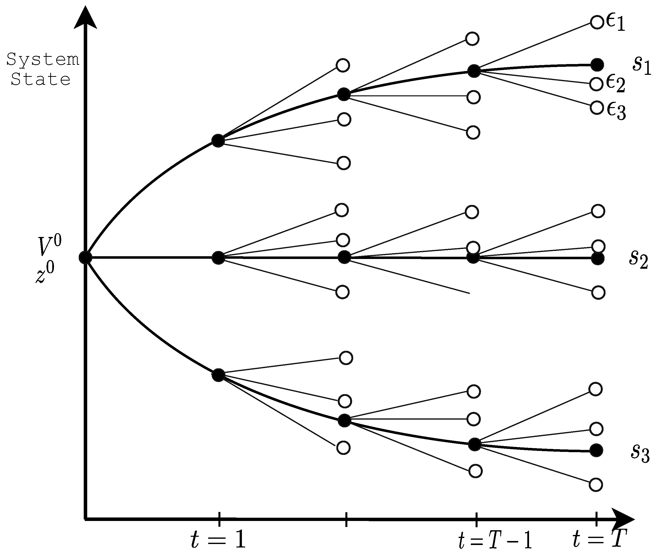
In the following, the parallel SDDP scheme used in this work is elaborated. We use a master process to designate the decomposed LP problems to a set of slave processes. In the SDDP scheme outlined in the previous section, the forward iteration is performed along $N_{\text{S}}$ forward samples. For each time stage in the backward iteration, the $N_{\text{B}}$ backward realizations are considered for each of the $N_{\text{S}}$ states obtained from the previous forward iteration. Thus, it is clear that the backward iteration is more computationally demanding, as it needs to solve $N_{\text{B}}$ as many LP problems as in the forward iteration. In other parallel implementations of SDDP applied to the LTHS problem, there seems to be (at least) two types of synchronization points; between stages in both the forward and backward iterations; see e.g., [7,12]. In this work, the presence of the synchronization points between stages in the backward iteration is challenged.

3.1. Forward Iteration

The forward iteration has to be completed before the backward cycle starts, so we get a synchronization point in between the two cycles. Furthermore, for each stage in the forward iteration along a sampled inflow scenario s, the LP problem corresponding to that stage is solved, and the resulting state variables (reservoir levels) are passed on to the next time stage to be evaluated along sample s. All of the $N_{\text{S}}$ LP problems formulated in each stage can be solved in parallel. However, due to the time-sequential coupling along scenario samples in the forward iteration, one cannot expect speedup in the forward iteration if the number of slave processors $N_P$ is greater than the number of forward scenarios $N_{\text{S}}$.

3.2. Backward Iteration

For each evaluated state in a stage t in the backward iteration, a Benders cut is created for stage $t-1$ by averaging contributions from the LP problems solved corresponding to the $N_{\text{B}}$ realizations of inflow. Each new inflow realization will in practice introduce a modest change in the right-hand side of the LP problem. Thus, the LP problem can normally be solved within a relatively low number of simplex iterations, provided that the previous solution basis is available. 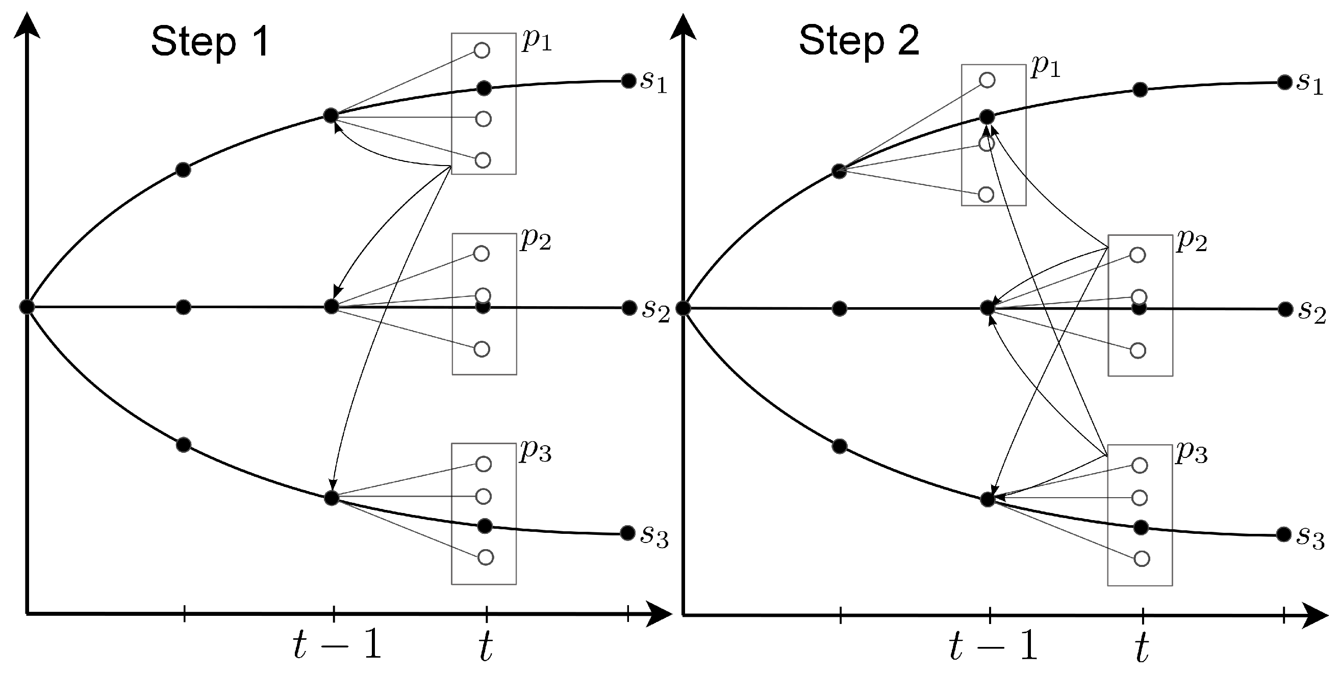In this work, the advantage of warm starting LP problems in the backward iteration was appreciated by letting a designated processor solve all $N_{\text{B}}$ problems originating from a given initial state. This is illustrated in Step 1 in Figure 2 with processors $p_1-p_3$. Allowing the $N_{\text{B}}$ realizations from a given state to be divided between different processors could add flexibility to the parallel processing scheme, but one would lose some of the warm start advantage. We have focused on limiting the communication between processors, and thus, the communication of the warm start basis was not considered.

Figure 2. Parallel processing scheme used in the backward iteration. Each of the processors $p_1-p_3$ solves $N_{\text{B}}$ linear programming (LP) problems and sends one cut to all states at stage $t-1$, as indicated by black arrows.

Figure 2. Parallel processing scheme used in the backward iteration. Each of the processors $p_1-p_3$ solves $N_{\text{B}}$ linear programming (LP) problems and sends one cut to all states at stage $t-1$, as indicated by black arrows.

The linear inflow model presented in Section 2 allows cuts to be shared among different states. This is illustrated in Step 1 in Figure 2, where the cut created for the state obtained following sample $s_1$ in stage $t-1$ is shared with the other states in that stage. Although convenient from an implementation point of view, it is not mathematically necessary to wait for all processors to create a cut for stage $t-1$ before continuing backwards in time to construct cuts for stage $t-2$; see [13] for a formal treatment of SDDP convergence properties. Each additional cut considered for stage t gives a better approximation to the future expected cost function $\mathsf{\alpha }\left(t\right)$. However, waiting for all cuts to be created forces all processors to be synchronized at each stage in the backward iteration. In the presented work, these stage-wise synchronization points in the backward iteration are relaxed, allowing each processor to wait for $N_{\text{W}}$ cuts, where $N_{\text{W}}\le N_{\text{S}}$. Let $N_{\text{W}}=1$ in Figure 2 and assume that processor $p_1$ computes its cut before $p_2$ and $p_3$ have finished. After communicating its cut to the master process, process $p_1$ is then flagged as available and will be assigned a new state at stage $t-2$ by the master process, as shown in Step 2 in Figure 2. By setting $N_W=1$, we fully relax the stage-wise synchronization points, and no processor is unused at any time during the backward phase. The cost of not waiting for all cuts may be slower convergence, as more iterations may be needed to converge.

4. Case Study

The SDDP model with the proposed parallel processing scheme was implemented in C++, using the dual simplex algorithm from the COIN-OR linear programming solver library for solving LP problems and the MPI protocol for message passing through the OpenMPI library. All simulations were carried out on a Linux cluster comprising 93 compute nodes, each with 2 × 6 core AMD processors at 2.4 GHz. The cluster operating system is CentOS 5.4.

The hydro system model used in this case study is based on a representation of the water course Nea-Nidelva in Norway comprising 12 hydro power plants with upstream reservoir capacity and with a total installed capacity of 536 MW. The reservoir sizes vary, ranging from annual to weekly storage. We estimated the stochastic inflow model from a historical inflow series for the area comprising 50 years of data, as shown in Figure 3. Inflows to individual reservoirs were scaled according to individual targets for expected annual inflow.

Normally, in a liberalized power market, a regional water course would be scheduled using exogenously-given stochastic price data, e.g., as described in [14]. However, to simplify the mathematical model, we considered it as an isolated system being scheduled together with thermal power production serving a time-varying load. Purchase of thermal power power was modeled by 70 steps, each characterized by a fixed capacity increment and a marginal cost, which is stepwise increasing. The system was created and tuned to obtain reasonable power prices and reservoir trajectories.

Figure 3. Historical inflow data used for fitting the stochastic inflow model. Values are in fractions of the maximum inflow value.

Figure 3. Historical inflow data used for fitting the stochastic inflow model. Values are in fractions of the maximum inflow value.

The system was simulated for 156 weeks, using a weekly stochastic time resolution and with seven sub-periods within each week. The decomposed LP problems have on average 777 variables and 98 constraints (excluding cuts). We tested the proposed parallelization scheme using two different combinations of forward samples $N_{\text{S}}$ and backward realizations $N_{\text{B}}$, as shown in Table 1. These settings are similar to those being used in many operational models. For both cases, we experimented with different numbers of processors ($N_{\text{P}}$) and cuts to wait for in the backward iteration ($N_{\text{W}}$). To ensure that the forward iteration did not become a bottleneck for parallel efficiency, the maximum number of slave processors was kept lower than or equal to the number of forward samples in both of the cases.

Table 1. Test case characteristics.

Cases	$N_{\text{S}}$	$N_{\text{B}}$	Max No. Processors	Serial CPU Time
Case 1	71	12	72	1 h 10 min
Case 2	200	50	144	5 h 3 min

Table 1. Test case characteristics.

Cases	$N_{\text{S}}$	$N_{\text{B}}$	Max No. Processors	Serial CPU Time
Case 1	71	12	72	1 h 10 min
Case 2	200	50	144	5 h 3 min

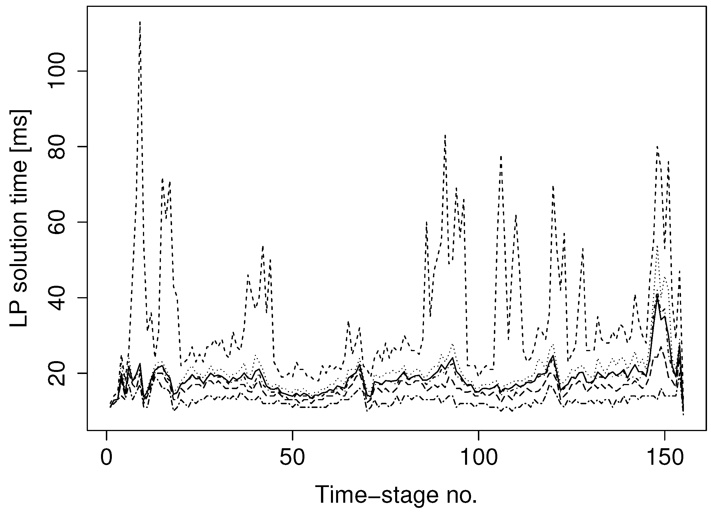
Relaxation of the stage-wise synchronization points in the backward iteration makes sense as long as LP solution times differ significantly between processors. We measured the time each processor spent solving all of its $N_{\text{B}}$ backward realizations in each time stage for a given backward iteration in Case 1. The distribution of solution times among different processors per time stage is shown in Figure 4. The figure displays the significant differences between the outliers (100 and zero percentiles) and the remaining measurements, represented by the 25, 50 and 75 percentiles. The large differences between the 100 and zero percentiles indicate that there is a potential for improving computational performance by relaxing the backward iteration stage wise synchronization points.

Figure 4. LP solution times (in milliseconds) per time stage in the backward iteration. The curves represent the 0, 25, 50, 75 and 100 percentiles.

Figure 4. LP solution times (in milliseconds) per time stage in the backward iteration. The curves represent the 0, 25, 50, 75 and 100 percentiles.

4.1. Parallel Efficiency

Generally, the gain achieved by applying parallel processing can be measured in terms of the efficiency of the parallel implementation when compared to the serial execution. Efficiency is defined as the ratio between the serial run-time on one core and the product of the parallel run-time on a number of cores divided by that number [15].

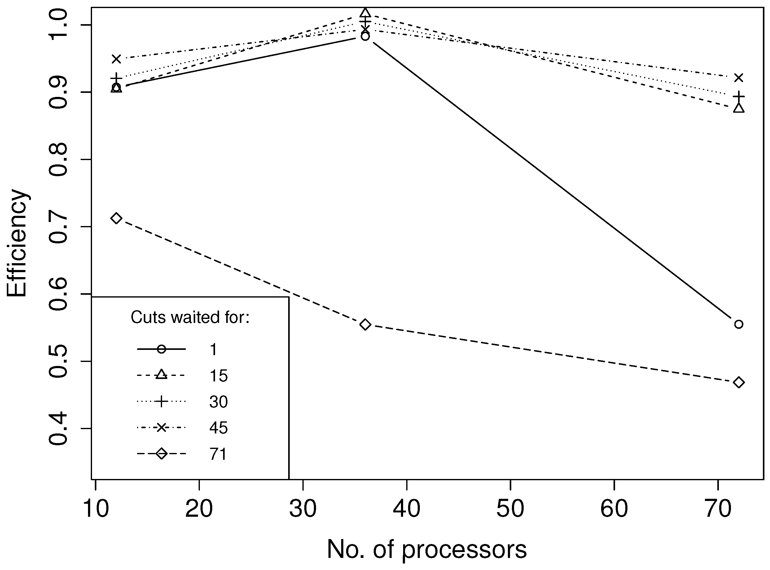
Each of the curves in Figure 5 and Figure 6 shows the parallel efficiency for different numbers of processors for a given value of $N_{\text{W}}$ for Cases 1 and 2, respectively. Waiting for all cuts, i.e., $N_{\text{W}}$ = 72 in Case 1 and $N_{\text{W}}$ = 200 in Case 2, serves as the base cases. 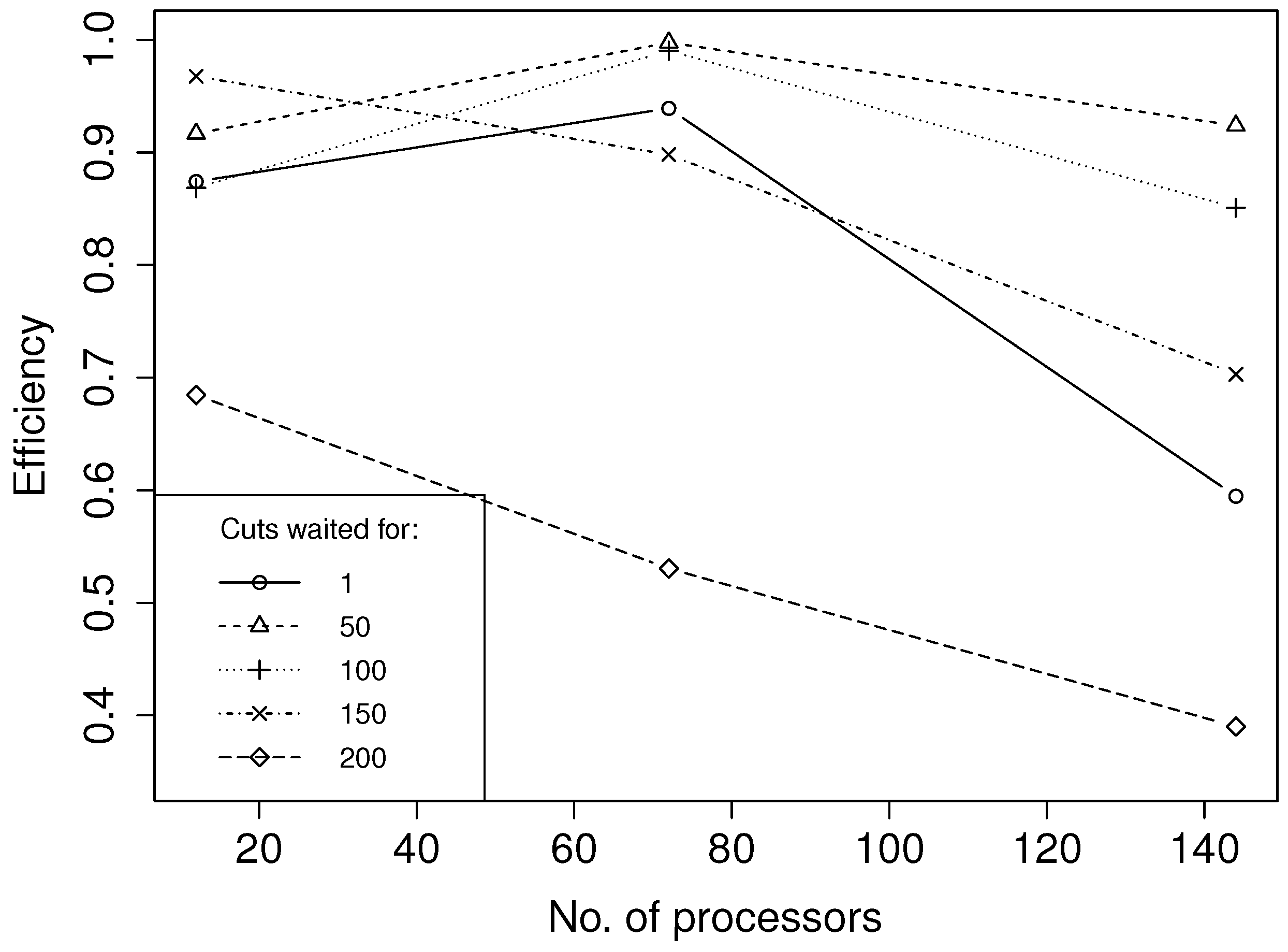Thus, we can measure the computational improvement in synchronization point relaxation against the base cases by inspecting Figure 5 and Figure 6. All data points represent averages of 10 independent runs. Results from both cases indicate that optimal parallel efficiency is obtained when partially relaxing the backward iteration stage-wise synchronization points. By keeping the synchronization points, we experienced a decreasing parallel efficiency with increasing number of processors. When partially relaxing the synchronization points, the parallel efficiency is maintained at a higher level with an increasing number of processors. Note that the low parallel efficiency shown in both cases when running at a maximum number of processors and with $N_{\text{W}}$ = 1 is due to the additional computation time caused by the slower convergence when only waiting for one cut.

Figure 5. Parallel efficiency as a function of the number of processors for Case 1. Each line corresponds to a separate choice of $N_{\text{W}}$.

Figure 5. Parallel efficiency as a function of the number of processors for Case 1. Each line corresponds to a separate choice of $N_{\text{W}}$.

Figure 6. Parallel efficiency as a function of the number of processors for Case 2. Each line corresponds to a separate choice of $N_{\text{W}}$.

Figure 6. Parallel efficiency as a function of the number of processors for Case 2. Each line corresponds to a separate choice of $N_{\text{W}}$.

4.2. Convergence

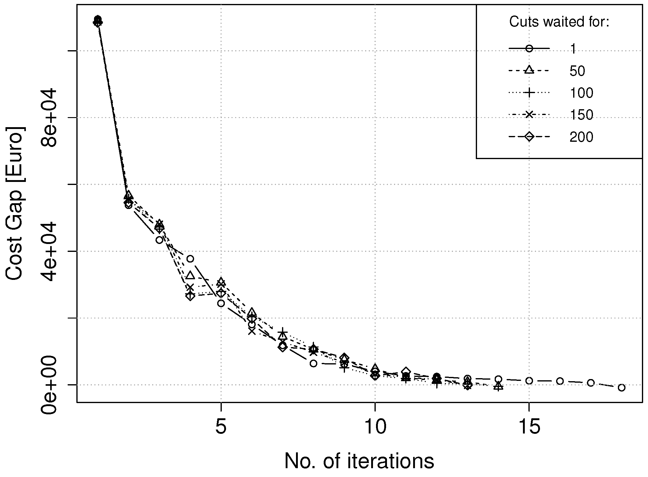
The increase in efficiency when relaxing the synchronization points implies that the convergence properties of the algorithm have not been dramatically changed. This implication is verified by looking at the cost gaps for Case 2 in Figure 7. Generally, lower values of $N_{\text{W}}$ result in higher numbers of iterations until the convergence criteria are met. This was as expected, since by decreasing $N_{\text{W}}$, each processor may have less cuts available at each stage and is therefore likely to have a less precise approximation of the future expected cost function. However, for the cases we have studied, the numbers of additional iterations needed when relaxing the synchronization points were modest.

Figure 7. Cost gap as a function of the number of iterations in the SDDP algorithm. The data are from Case 2, with $N_{\text{P}}=144$ and with different values of $N_{\text{W}}$.

Figure 7. Cost gap as a function of the number of iterations in the SDDP algorithm. The data are from Case 2, with $N_{\text{P}}=144$ and with different values of $N_{\text{W}}$.

5. Conclusions

A parallel processing scheme for the SDDP algorithm applied to the LTHS problem was presented. In contrast to traditional parallel schemes used with the SDDP algorithm, the stage-wise synchronization points in the backward iteration are relaxed. Thus, each processor does not need to wait for all processors to complete their jobs before starting a new job. Since the expected generator schedules should not be affected by the synchronization point relaxation, the sole benefit of introducing the relaxation can be measured in terms of improved computational performance.

A case study based on a Norwegian watercourse was established for the purpose of testing the parallel processing scheme. The test results show that the parallel efficiency significantly improves when partially relaxing the backward iteration synchronization points. In between synchronization and full relaxation, the optimal number of processors to wait for balances the trade-off between a precise approximation of the future expected cost function and processor waiting time. Results from two different test cases show that the optimal number of cuts to wait for is case dependent.

The case study reflect a simplified version of operational data, both in terms of system size and physical details being modeled. However, we believe that the presented case study results demonstrate a significant potential for improvement in the parallel efficiency of operational SDDP models.