Representational Learning for Fault Diagnosis of Wind Turbine Equipment: A Multi-Layered Extreme Learning Machines Approach ^†

Abstract

Reliable and quick response fault diagnosis is crucial for the wind turbine generator system (WTGS) to avoid unplanned interruption and to reduce the maintenance cost. However, the conditional data generated from WTGS operating in a tough environment is always dynamical and high-dimensional. To address these challenges, we propose a new fault diagnosis scheme which is composed of multiple extreme learning machines (ELM) in a hierarchical structure, where a forwarding list of ELM layers is concatenated and each of them is processed independently for its corresponding role. The framework enables both representational feature learning and fault classification. The multi-layered ELM based representational learning covers functions including data preprocessing, feature extraction and dimension reduction. An ELM based autoencoder is trained to generate a hidden layer output weight matrix, which is then used to transform the input dataset into a new feature representation. Compared with the traditional feature extraction methods which may empirically wipe off some “insignificant’ feature information that in fact conveys certain undiscovered important knowledge, the introduced representational learning method could overcome the loss of information content. The computed output weight matrix projects the high dimensional input vector into a compressed and orthogonally weighted distribution. The last single layer of ELM is applied for fault classification. Unlike the greedy layer wise learning method adopted in back propagation based deep learning (DL), the proposed framework does not need iterative fine-tuning of parameters. To evaluate its experimental performance, comparison tests are carried out on a wind turbine generator simulator. The results show that the proposed diagnostic framework achieves the best performance among the compared approaches in terms of accuracy and efficiency in multiple faults detection of wind turbines.

1. Introduction

Wind turbine generator systems (WTGS) are the fastest-growing applications in renewable power industry. The structure of WTGS is complex, its reliability becomes an important issue. As wind power generators are widely mounted on high mountains or offshore islands, it is costly for routine maintenance [1]. Continuously condition monitoring and fault diagnosis technologies are therefore necessary so as to reduce unnecessary maintenance cost and keep system working reliably without unexpected shutdown. 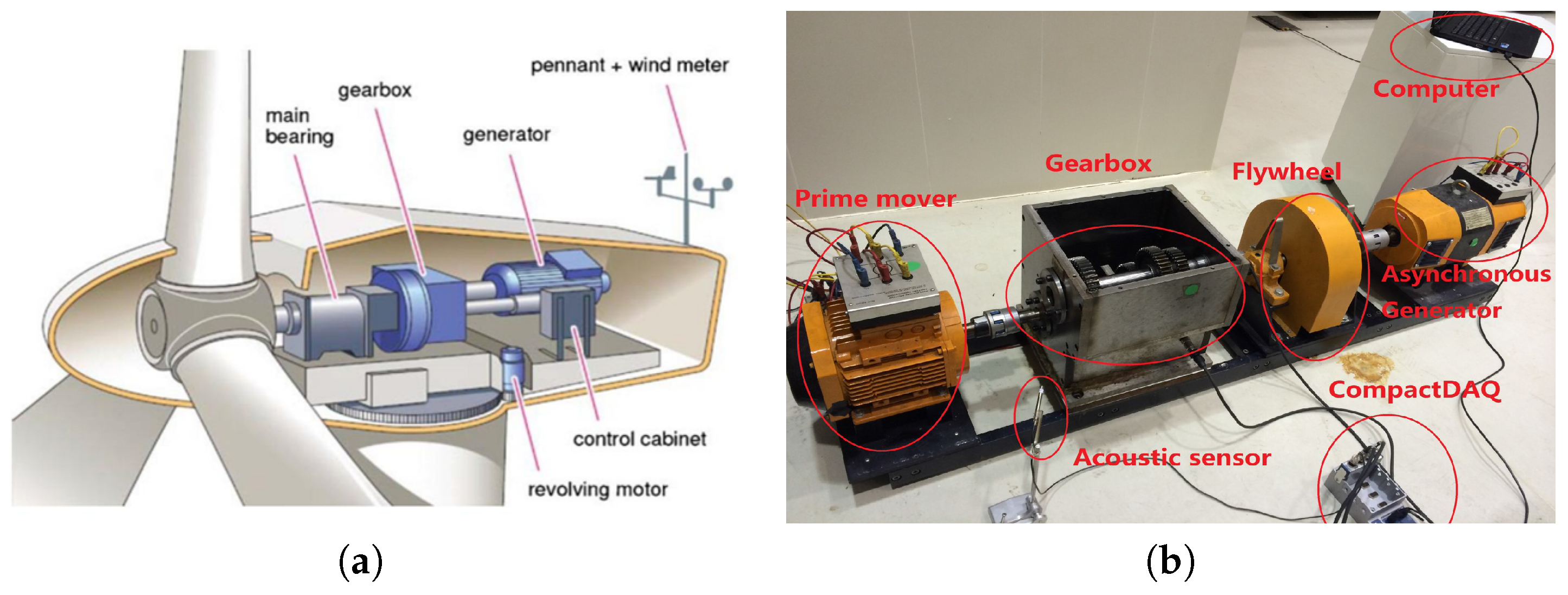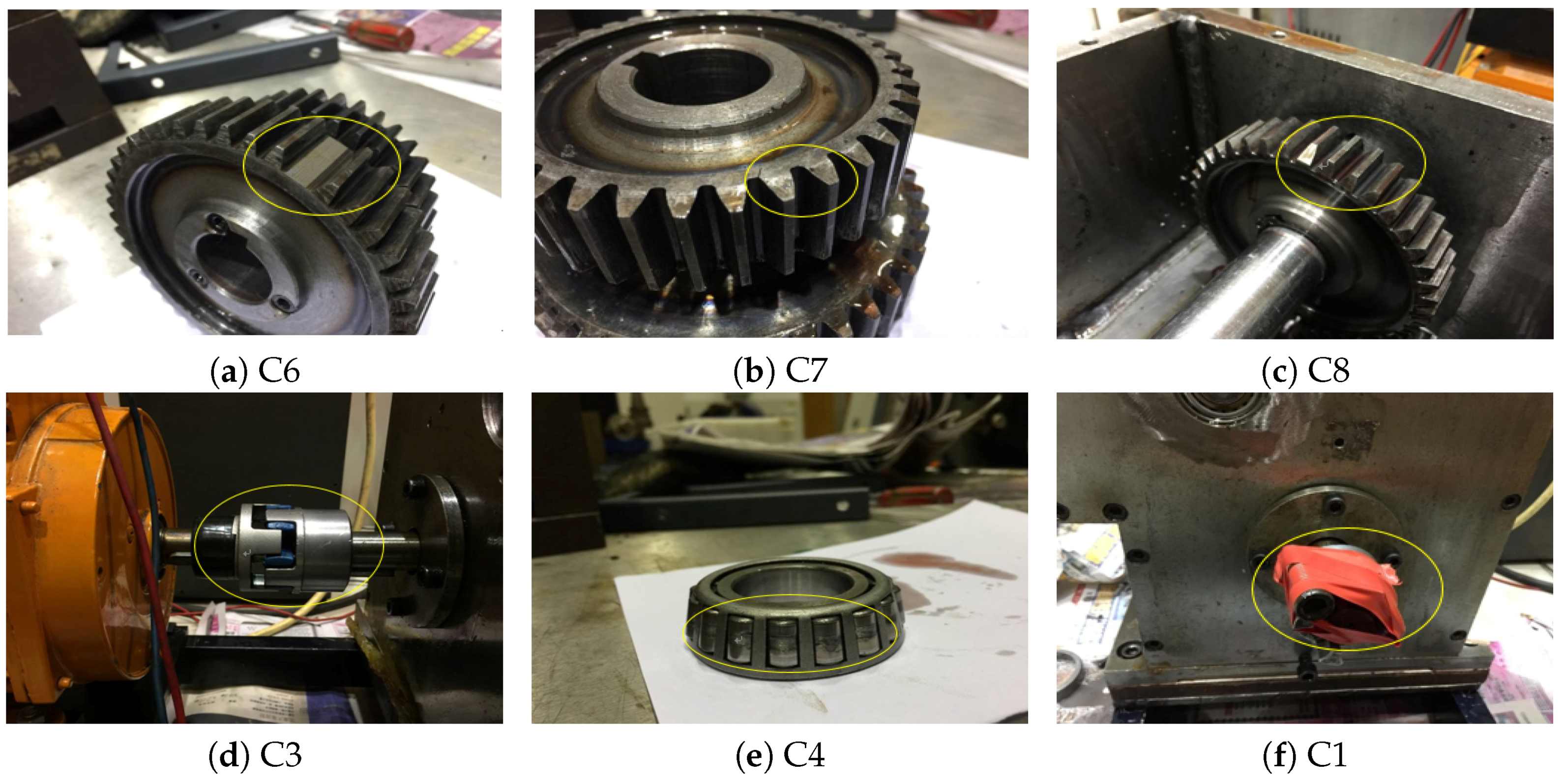A typical WTGS includes gearbox, power generator, control cabinet and rotary motor, etc., (as shown in Figure 1a), where the gearbox is statistically more vulnerable compared with other components. It shed light upon the importance of the condition monitoring of gearbox. More specifically, the faults of gearbox mainly results from two major components: gears and bearings, which include broken tooth, chipped tooth, wear-off of outer race or rolling elements of bearing, etc. [2]. Real-time monitoring and fault diagnosis aim to detect and identify any potential abnormalities and faults, so as to take corresponding actions to avoid serious component damage or system disaster.

Nowadays, a large body of research shows that fault detection based on a machine learning-based approach is feasible. Machine learning methods, such as neural networks (NNs), support vector machine (SVM) and deep learning (DL) may be promising solutions to classify the normal and abnormal patterns. A brief workflow of machine learning methods for fault diagnosis includes analog signal acquisition, data pre-processing and pattern recognition. Regarding the feature information sources (e.g., vibration signals, acoustic and temperature signals), the vibration signals are often adopted for their ease of acquisition and sensitivity to a wide range of faults. Moreover, intelligent fault diagnosis of WTGS relies on the effectiveness of signal processing and classification methods. The raw vibration signals contain high-dimensional information and abundant noise (includes irrelevant and redundant signals), which cannot be feasibly fed into the fault diagnostic system directly [3]. Many studies focus on the improvement of data pre-processing and feature extraction from the raw vibration signals [4,5]. Generally, a good intermediate representation method is required to retain the information of its original input, while at the same time being consistent to a given form (i.e., a real-valued vector of a given size in case of an autoencoder) [6]. Therefore, it is essential to extract the compact feature information from raw vibration signals. The data processing method simplifies the computational expense and benefits the improvement of the generation performance. Some typical feature extraction methods, such as wavelet packet transform (WPT) [7,8,9,10], empirical mode decomposition (EMD) [11], time-domain statistical features (TDSF) [12,13] and independent component analysis (ICA) [14,15,16,17] have been proved to be equivalent to a large-scale matrix factorization problem (i.e., there may be still some irrelevant or redundant noise in the extracted features) [18]. In order to resolve this problem, a feature selection method could be employed to wipe off irrelevant and redundant information so that the dimension of extracted feature is reduced. Typical feature selection approaches include compensation distance evaluation technique (CDET) [19], principal component analysis (PCA) and kernel principal component analysis (KPCA) [16,20,21] and the genetic algorithm (GA) based methods [22,23,24]. However, these linear methods have a common shortcoming in an attempt to extract nonlinear characteristics, which may result in a weak performance in the downstream pattern recognition process.

The raw vibration signals obtained from WTGS are characterized with high dimensional and nonlinear patterns, which is difficult for direct classification. In order to extract the features from the raw vibration signals, this paper introduces the concept of autoencoder and explores its application. Unlike PCA and its variants, autoencoder does not impose the dictionary elements be orthogonal, which makes it flexible to be adapted to the fluctuation in data representation [18]. In the structure of autoencoder, each layer in the stack architecture can be treated as an independent module [25]. The procedure shows briefly as follows. Each layer is firstly trained to produce a new (hidden) representation of the observed patterns (input data). It optimizes a local supervised criterion based on its received input representation from forehead layer. Each layer $L_i$ produces a new representation that is more abstract than the previous level $L_{i-1}$ [6]. After representational learning for a feature mapping that produces a high level intermediate representations (e.g., a high-dimensional intermediate matrix) of the input pattern, whereas, it is still complex and hard to compute directly. Therefore, it is necessary to decode the high-dimensional representations into a relatively low-dimensional and simple representations. Currently, there are only very limited algorithms that could work well for this purpose: restricted boltzmann machines (RBMs) [26,27,28] trained with contrastive divergence on one hand, and various types of autoencoders on the other. Regarding algorithms for classification, artificial neural networks (ANN) and multi-layer perception (MLP), are widely used for fault diagnosis of rotating machinery [3,29,30]. However, MLP has inevitable drawbacks which mainly reflects in local minima, time-consuming and over-fitting. Additionally, most classifiers are designed for binary classification. Regarding multiclass classification, the common methods actually employ a combination of binary classifiers with one-versus-all (1va) or one-versus-one (1v1) strategies [3]. Obviously, the combination with many binary classifiers increases computational burden and training time. Nowadays, researches show that SVM works well at recognizing the rotating equipment faults [31,32]. Compared with early machine learning methods, global optimum and relatively high generalization performance are the obvious advantages of SVM, while it has the same demerits with MLP, namely, time-consuming and local minimal. Considering that more than one type of fault may co-exist at the same time, it may be significant to propose a classifier which could offer the probabilities of all possible faults. In order to realize this assumption, the probabilistic neural network (PNN) [33,34] is employed as a probabilistic classifier. It is testified that the performance of PNN is superior to the SVM based method [29]. It trained a probabilistic classifier with a model using the Bayesian framework. However, the work [29] failed to explain clearly the principle of decision threshold. The value of decision threshold depends on some specific validation datasets and is not generally applicable for other areas.

Recent studies show that extreme learning machines (ELM) has better scalability and achieves much faster learning speed than SVM [35,36]. From the structural point of view, ELM is a multi-input and multi-output or single-output structure with single-hidden layer feedforward networks (SLFNs). Thus, ELM algorithm is more appropriate to multiclass classification. This paper extends the capability of ELM to the scope of feature learning, and proposes a multi-layered ELM network for feature learning and fault diagnosis. This paper proposes an ELM based autoencoder for feature mapping, and then the new representations are fed into the ELM based classifier for multi-label recognition. The proposed multi-layered ELM network consists of an ELM based autoencoder, dimension transformation, and supervised feature recognition. The autoencoder and dimension transform reconstruct the raw data into three types of representation (i.e., compressed, equal and sparse dimension). The original ELM classifier is applied for the final decision making.

The paper is organized as follows. Section 2 presents the structure of the proposed fault diagnostic framework and the involved algorithms. Experimental rig setup and signals sample data acquisition with a simulated WTGS are implemented in Section 3. Section 4 discusses the experimental results of the framework and its comparisons with other methods including SVM and ML-ELM. Section 5 concludes the study.

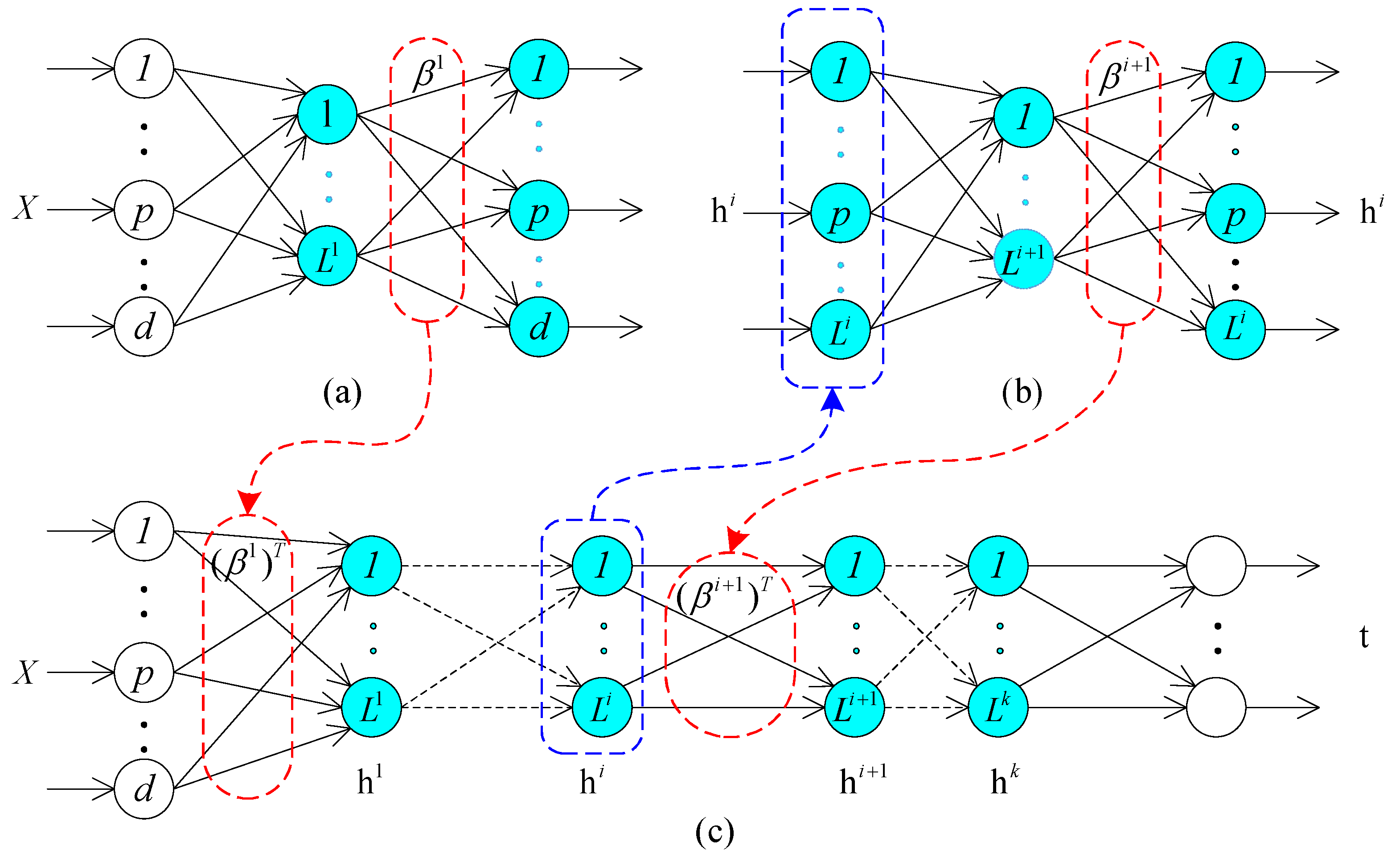
2. The Proposed Fault Diagnostic Framework

As shown in Figure 2, the proposed fault diagnosis framework is divided into three submodules: (a) ELM based autoencoder for feature extraction; (b) Matrix compression for dimension reduction; and (c) ELM based classifier for fault classification. The ELM based autoencoder enables three scales of data transformations and representations. Firstly, the raw dataset, which is usually in the form of a high-dimensional matrix, is fed into autoencoder. The autocoder network could be trained using multi-layered ELM networks, each of which is set with a different number of hidden layer nodes L. The dimension of the output layer is set to equal with the input dataset. The output weight vector $\mathsf{\beta }$ is calculated in the ELM output mapping. Secondly, the dimensional transformation compresses the output of autoencoder with a simple matrix transform. The raw dataset is thus converted into a low-dimensioned feature matrix, which is described in detail in Section 2.2. In order to optimize the number of hidden-layer nodes L, a method using multiple sets of contrast tests is introduced in Section 3.2. Finally, one classic ELM classification slice is applied for the final decision making with the input of the converted feature matrix. It is notable that the number of hidden-layer nodes is the only adjustable parameter in the proposed method. The two weighting vectors $\mathsf{\beta }$ and $\mathsf{\delta }$ are independent in two ELM networks (ELM-based autoencoder and ELM classifier). The former one is applied for regression, while the later is used for classification.

2.1. Extreme Learning Machines Based Autoencoder

ELM is a recently prevailing machine learning method that has been successfully adopted for various applications [37,38]. ELM is characterized with its single hidden layer structure, of which the parameters are initialized randomly. The parameters of the hidden layer are independent upon the target function and the training dataset [39,40]. The output weights which link the hidden layer to output layer are determined analytically through a Moore-Penrose generalized inverse [37,41]. Benefited from its simple structure and efficient learning algorithm, ELM owns very good generalization capability superior to the traditional ANN and SVM. The basics of ELM is summarized as follows:

$$\begin{array}{c}{f}_L(\mathbf{x})={\displaystyle \sum _{i=1}^L}{\mathsf{\beta }}_i{h}_i(\mathbf{x})=\mathbf{h}(\mathbf{x})\mathsf{\beta }\hfill \\ \left\{\begin{array}{c}\mathsf{\beta }={\left[{\mathsf{\beta }}_1,...,{\mathsf{\beta }}_L\right]}^{\mathrm{T}}\hfill \\ h(\mathbf{x})=[g_1(\mathbf{x}),...,g_L(\mathbf{x})]\hfill \end{array}\right.\hfill \end{array}$$

(1)

where ${\mathsf{\beta }}_i$ is the output weight vector between the hidden nodes and the output nodes. $h(\mathbf{x})$ is the hidden nodes output for the input $\mathbf{x}$ and $g_i(\mathbf{x})$ is the i-th hidden node activation function.

Given the N training samples ${\left\{(x_i,t_i)\right\}}_{i=1}^N$, the ELM is to resolve the follow problems:

$$\mathbf{H}\mathsf{\beta }=\mathbf{T}$$

(2)

where $\mathbf{T}={[t_1,...,t_N]}^{\mathrm{T}}$ is the target labels, the matrix $\mathbf{H}={[{\mathbf{h}}^{\mathrm{T}}(x_1),...,{\mathbf{h}}^{\mathrm{T}}(x_N)]}^{\mathrm{T}}$ is the hidden nodes output.

The output weight vector $\mathsf{\beta }$ can be calculated by Equation (3),

$$\mathsf{\beta }={\mathbf{H}}^{†}\mathbf{T}$$

(3)

where ${\mathbf{H}}^{†}$ is the Moore-Penrose generalized inverse of matrix $\mathbf{H}$.

In order to obtain better generalization performance and to make the solution more robust, a positive constraint parameter $\frac{1}{C}$ is added to the diagonal of ${\mathbf{H}}^{\mathbf{T}}\mathbf{H}$ in the calculation of the output weight, as shown in Equation (4).

$$\mathsf{\beta }={(\frac{1}{C}+{\mathbf{H}}^{\mathbf{T}}\mathbf{H})}^{-1}{\mathbf{H}}^{\mathbf{T}}\mathbf{T}$$

(4)

To perform autoencoding and feature representation, the ELM algorithm is modified as follows: the target matrix is set equally to the input data, namely, $\mathbf{t}=\mathbf{x}$. The random assigned input weights and biases of the hidden nodes are chosen to be orthogonal. Widrow [42] introduced a Least Mean Square (LMS) method implementation for ELM and a corresponding ELM based autoencoder in which non-orthogonal random hidden parameters (i.e., weights and biases) are used. However, orthogonalization of randomly generated hidden parameters tends to improve the generalization performance of ELM autoencoder. Generally, the objective of ELM based autoencoder is to represent the input features meaningfully in the following three optional representations:

(1)

Compressed representation: represent features from a high dimensional input data space to a low dimensional feature space;

(2)

Sparse representation: represent features from a low dimensional input data space to a high dimensional feature space;

(3)

Equal representation: represent features from an input data space dimension equal to feature space dimension.

Figure 3 shows the structure of random feature mapping. In an ELM based autoencoder, the orthogonal random weight matrix and biases of the hidden nodes project the input data to a different or equal dimensional space as shown by Johnson-Lindenstrauss Lemma and calculated by Equation (5):

$$\begin{array}{c}\mathbf{h}=g(\mathbf{a}\mathbf{x}+\mathbf{b}),{\mathbf{a}}^{\mathrm{T}}\mathbf{a}=\mathbf{I},{\mathbf{b}}^{\mathrm{T}}\mathbf{b}=1\hfill \end{array}$$

(5)

where $\mathbf{a}={[{\mathbf{a}}_1,...,{\mathbf{a}}_L]}^{\mathrm{T}}$ are the orthogonal weight vector and $\mathbf{b}={[{\mathbf{b}}_1,...,{\mathbf{b}}_L]}^{\mathrm{T}}$ is the orthogonal random bias vector between the input layer and hidden layer.

The output weight $\mathsf{\beta }$ of ELM based autoencoder is applied for learning the transformation from input dataset to the feature space. For sparse and compressed representation, output weight $\mathsf{\beta }$ is calculated by Equation (6),

$$\mathsf{\beta }={(\frac{1}{\mathbf{C}}+{\mathbf{H}}^{\mathrm{T}}\mathbf{H})}^{-1}{\mathbf{H}}^{\mathrm{T}}\mathbf{X}$$

(6)

where the vector $\mathbf{X}={[{\mathbf{x}}_1,...,{\mathbf{x}}_N]}^{\mathrm{T}}$ is the input data and output data, the input data equals to the output in proposed autoencoder.

For equal dimension representations, the output weight $\mathsf{\beta }$ is calculated by Equation (7),

$$\begin{array}{c}\mathsf{\beta }={\mathbf{H}}^{-1}\mathbf{X}and{\mathsf{\beta }}^{\mathrm{T}}\mathsf{\beta }=\mathbf{I}\hfill \end{array}$$

(7)

2.2. Dimension Compression

This paper adopts the regression method to train the parameters of the autoencoder. However, the above transform is not enough for the data preprocessing, because the dimension of input data does not decrease (see Equation (2) and let $\mathbf{t}=\mathbf{x}$). The output data with equal dimension of input data cannot reduce the complexity of the post classifier. After all the parameters of autoencoder are identified, this paper applies a transform to represent the input data. The eventual representation vector shows in Equation (8),

$$Y_L(\mathbf{x})={(\mathsf{\beta }{f}_L(\mathbf{x}))}^{\mathrm{T}}={(\mathsf{\beta }\mathbf{X})}^{\mathrm{T}}$$

(8)

where $Y_L(\mathbf{x})$ is the final output of autoencoder. The dimension of $Y_L(\mathbf{x})$ is shown as Equation (9). The subscripts N and L represent the number of input samples and hidden layer nodes, respectively.

$$Y_L(\mathbf{x})=\left[\begin{array}{ccc}{Y}_1(\mathbf{x})& \dots & Y_L(\mathbf{x})\end{array}\right]=\left[\begin{array}{ccc}{Y}_1(x_1)& \dots & Y_L(x_1)\\ ⋮& ⋮& ⋮\\ Y_1(x_N)& \dots & Y_L(x_N)\end{array}\right]$$

(9)

From the Equations (8) and (9), the procedure from the high-dimensional vector to the low-dimensional vector can be explained that each element in sample data ${\mathbf{x}}_{i(i\in N)}$ has relationship with $\mathsf{\beta }$, in other words, $\mathsf{\beta }$ can be seen as a weight distribution of ${\mathbf{x}}_{i(i\in N)}$. The procedure from ${\mathbf{x}}_{i(i\in N)}$ to $Y_L(\mathbf{x})$ is an unsupervised learning as the parameters have been identified in the first part as shown in Figure 2.

Unlike the concept of DL-based autoencoder, the proposed ELM-based autoencoder shows differences at the following four aspects:

(1)

The proposed autoencoder is a ELM based network composing of a set of single-hidden-layer slice, whereas the DL-based autoencoder is a multiple hidden layers network.

(2)

DL tends to adopt BP algorithm to train all parameters of autoencoder, differently, this paper employs the ELM to configure the network with supervised learning (i.e., Let the output data equal to input data, $\mathbf{t}=\mathbf{x}$). We can get the final output weight $\mathsf{\beta }$ so as to transform input data into a new representation through Equation (8). The dimension of converted data is much smaller than the raw input data.

(3)

The DL-based autoencoder tends to map the input dataset into high-dimensional sparse features. While this research applies a compressed representation of the input data.

(4)

The DL-based autoencoder trained with BP algorithm is a really time-consuming process as it requires intensive parameters setting and iterative tuning. On the contrary, each ELM slice in the multi-layered ELM based autocoder can be seen as an independent feature extractor, which relies only on the feature output of its previous hidden layer. The weights or parameters of the current hidden layer could be assigned randomly.

2.3. ELM for Classification

Regarding the binary classification problems, the decision function of ELM is:

$$f_L(\mathbf{x})=\mathbf{sign}[\mathbf{h}(\mathbf{x})\mathsf{\delta }]$$

(10)

Unlike other learning algorithms, ELM tends to reach not only the smallest training error but also the smallest norm of output weights. Bartlett’s theory [7,43] mentioned that if a neural network is used for a pattern recognition problem, the smaller size of weights brings a smaller square error during the training process, and then realizes a better generalization performance, which doesn’t relate directly to the number of nodes. In order to reach smaller training error, the smaller the norms of weights tend to have a better generalization performance. For a m-label classification case, ELM aims to minimize the training error as well as the norm of the output weights. The problem can be summarized as:

$$\mathbf{Minimize}:||\mathbf{H}\mathsf{\delta }-T|{|}^{2}and||\mathsf{\delta }||$$

(11)

where $\mathsf{\delta }={\left[{\mathsf{\delta }}_1,...,{\mathsf{\delta }}_l\right]}^{\mathrm{T}}$ is the vector of the output weight between the hidden layer of l-nodes and the output nodes.

$$\mathbf{H}=\left[\begin{array}{c}\mathbf{h}({\mathbf{x}}_1)\\ ⋮\\ \mathbf{h}({\mathbf{x}}_N)\end{array}\right]=\left[\begin{array}{ccc}{h}_1({\mathbf{x}}_1)& \dots & h_l({\mathbf{x}}_1)\\ ⋮& ⋮& ⋮\\ h_1({\mathbf{x}}_N)& \dots & h_l({\mathbf{x}}_N)\end{array}\right]$$

(12)

where $\mathbf{h}\left(\mathbf{x}\right)={\left[h_1\left(\mathbf{x}\right),...,h_l\left(\mathbf{x}\right)\right]}^{\mathrm{T}}$ is the output vector of the hidden layer which maps the data from the d-dimensional input space to the l-dimensional hidden-layer space $\mathbf{H}$ , $\mathbf{T}$ is the training data target matrix.

$$\mathbf{T}=\left[\begin{array}{c}{\mathbf{t}}_1^{\mathrm{T}}\\ ⋮\\ {\mathbf{t}}_N^{\mathrm{T}}\end{array}\right]=\left[\begin{array}{ccc}{t}_{11}& \dots & t_{1m}\\ ⋮& ⋮& ⋮\\ t_{N1}& \dots & t_{Nm}\end{array}\right]$$

(13)

In the binary classification case, ELM has just a single output node. The optimal output value is chosen as the predicted output label. However, for a multiclass identification problem, this binary classification method could not be applied directly. There are two conditions for multilabel classification:

(1)

If the ELM only has a single-output node, among the multiclass labels, ELM selects the most closed value as the target label. In this case, the ELM solution to the binary classification case becomes a specific case of multiclass solution.

(2)

If the ELM has multi-output nodes, the index of the output node with the highest output value is considered as the label of the input data.

According to the conclusion of study [35], the single-output node classification can be considered a specific case of multi-output nodes classification when the number of output nodes is set to 1. This paper discuss only the multi-output case.

If the original number of class labels is P, the expected output vector of the M-output nodes is ${\mathbf{t}}_i={[0,...,0,\stackrel{P}{1},...,\stackrel{M}{0}]}^{\mathrm{T}}$. In this case, only the P-th elements of ${\mathbf{t}}_i={[t_{i,1},...,t_{i,M}]}^{\mathrm{T}}$ is set to 1, while the rest is set to 0. The classification problem (see Equation (11)) for ELM with multi-output nodes can be formulated as Equation (14),

$$\begin{array}{c}\mathbf{Minimize}:L_{P_{\text{ELM}}}=\frac{1}{2}{||\mathsf{\delta }||}^2+C\frac{1}{2}\sum _{i=1}^N||{\xi }_i|{|}^2\hfill \\ \mathbf{s}.\mathbf{t}.\mathbf{h}({\mathbf{x}}_i)\mathsf{\delta }={\mathbf{t}}_i^{\mathrm{T}}-{\xi }_i^{\mathrm{T}},\left(i=1,...,N\right)\hfill \end{array}$$

(14)

where ${\xi }_i={[{\xi }_{i,1},...,{\xi }_{i,M}]}^{\mathrm{T}}$ is the training error vector of the M-output nodes with respect to the training sample ${\mathbf{x}}_i$.

Based on the Karush-Kuhn-Tucker (KKT) theorem, to train ELM is equivalent to solve the following dual optimization problem:

$$L_{D_{\text{ELM}}}=\frac{1}{2}{||\mathsf{\delta }||}^2+C\frac{1}{2}\sum _{i=1}^N||{\xi }_i|{|}^2-\sum _{i=1}^N\sum _{j=1}^M{\mathsf{\alpha }}_{i,j}(\mathbf{h}({\mathbf{x}}_i){\mathsf{\delta }}_j-t_{i,j}+{\xi }_{i,j})$$

(15)

We can have the KKT corresponding optimality conditions as follows:

$$\frac{\partial L_{D_{\text{ELM}}}}{\partial {\mathsf{\beta }}_j}=0\to {\mathsf{\delta }}_j=\sum _{i=1}^N{\mathsf{\alpha }}_{i,j}(\mathbf{h}{({\mathbf{x}}_i)}^{\mathrm{T}}\to \mathsf{\delta }={\mathbf{H}}^{\mathrm{T}}a$$

(16)

$$\frac{\partial L_{D_{\text{ELM}}}}{\partial {\xi }_i}=0\to {\mathsf{\alpha }}_i=C{\xi }_i,i=1,...,N$$

(17)

$$\frac{\partial L_{D_{\text{ELM}}}}{\partial {\mathsf{\alpha }}_i}=0\to \mathbf{h}({\mathbf{x}}_i)\mathsf{\delta }-t_i^T+{\xi }_i^{\mathrm{T}},i=1,...,N$$

(18)

where ${\mathbf{a}}_i={[{\mathsf{\alpha }}_{i,1},...,{\mathsf{\alpha }}_{i,M}]}^{\mathrm{T}}$. In this case, by substituting Equations (16) and (17) into Equation (18), the aforementioned equations can be equivalently written as:

$$(\frac{1}{C}+\mathbf{H}{\mathbf{H}}^{\mathrm{T}})\mathsf{\alpha }=\mathbf{T}$$

(19)

From Equations (16)–(19), we have:

$$\mathsf{\delta }={\mathbf{H}}^{\mathrm{T}}{(\frac{1}{C}+\mathbf{H}{\mathbf{H}}^{\mathrm{T}})}^{-1}\mathbf{X}$$

(20)

The output function of ELM classifier shows:

$$\mathbf{f}(\mathbf{x})=\mathbf{h}(\mathbf{x})\mathsf{\delta }=\mathbf{h}(\mathbf{x}){\mathbf{H}}^{\mathrm{T}}{\left(\frac{1}{C}+\mathbf{H}{\mathbf{H}}^{\mathrm{T}}\right)}^{-1}\mathbf{T}$$

(21)

For multiclass cases, the predicted class label of a given testing sample is the index number of the output node which has the highest output value for the given testing sample. Let $f_j(\mathbf{x})$ denoted the output function of the j-th output node (i.e., $f_j(\mathbf{x})={[f_1(\mathbf{x}),...,f_M(\mathbf{x})]}^{\mathrm{T}}$), and then the predicted class label of sample $\mathbf{x}$ is:

$$\mathbf{Label}(\mathbf{x})=arg\underset{i\in \{1,...,M\}}{max}{f}_i(\mathbf{x})$$

(22)

In short, there are very few parameters required to set in ELM algorithm. If the feature mapping $\mathbf{h}(\mathbf{x})$ is already known, only one parameter C needs to be specified. The generalization performance of ELM is not sensitive to the dimensionality l of the feature space (i.e., the number of hidden nodes) as long as l is not set to be too small. Different from SVM which usually requests to specify two parameters (C,$\mathsf{\gamma }$), single-parameter setting makes ELM easy and efficient in the computation for feature representation.

2.4. General Workflow

Table 1. The ELM training algorithm.

The ELM Training Algorithm
Step1, Initializing the hidden nodes L;
Step2, Randomly assign input weight $\mathsf{\omega }$ and bias $\mathbf{b}$;
Step3, Calculate the hidden layer output matrix $\mathbf{H}$;
Step4, Calculate the output weight vector $\mathsf{\beta }$;
Step5, Calculate the matrix $Y_L(x_N)$ (as shown in eqs (8) and (9));
Step6, Initializing the hidden nodes l;
Step7, Randomly assign input weight $\widehat{\mathsf{\omega }}$ and bias $\widehat{\mathbf{b}}$;
Step8, Calculate the hidden layer output matrix $\widehat{\mathbf{H}}$;
Step9, Calculate the output weight matrix $\mathsf{\delta }$.

summarizes the ELM training algorithm. The flowchart of the proposed fault diagnostic system for WTGS shows in Figure 4. It consists of three components, namely, (a) signal acquisition module; (b) feature extraction module; (c) fault identification module. For the signal acquisition module, the real-time dataset ${\mathbf{x}}_{\text{new}}$ acquisition model uses accelerometers to record the vibration signals of the WTGS. Two tri-axial accelerometers are mounted on the outboard of the gearbox along with the shaft transmission, in order to acquire the vibration signals along the horizontal and vertical directions respectively. The training dataset $D_{\text{train}}$ and testing dataset $D_{\text{test}}$ are recorded from experiment by accelerometers. In this paper, the real-time signal is processed by the data pre-processing approaches (i.e., ${\mathbf{x}}_{\text{new}}$ is converted into ${\mathbf{x}}_{\text{proc}}$), which is identified by the simultaneous fault diagnostic model. In feature extraction module, ELM based autoencoder is employed to generate the most important information ($D_{\text{AE\_train}}$ and $D_{\text{AE\_test}}$) of the input dataset ($D_{\text{train}}$ and $D_{\text{test}}$). In order to avoid domination of largest feature values, $D_{\text{AE\_train}}$ and $D_{\text{AE\_test}}$ are normalized into $D_{\text{nor\_train}}$ and $D_{\text{nor\_test}}$ which are within [0, 1]. After feature extraction and normalization, the datasets $D_{\text{nor\_train}}$ and $D_{\text{nor\_test}}$ are sent into classifier for fault recognition. Regarding the real application of this method, the proposed scheme can be seen as a fault pattern indicator in the whole wind forms protection system. First, the real-time vibration signals are collected by accelerators installed on transmission case, and then the vibrations signals are converted into voltage signals and sent into sampling unit. The sampling unit modulates these signals and sends the processed signals into recognition unit. Compared with the proposed scheme, the functions of vibration signals acquisition unit and sampling unit equal to the module (a) in Figure 4. Second, the pattern recognition unit extracts the input signals and classifies them into different labels, and then outputs single or multilabels to the decision making unit. The function of pattern recognition unit equals to the modules (b) and (c) in Figure 4.

3. Case Study and Experimental Setup

To verify the effectiveness of the proposed fault diagnostic framework for WTGS, experimental test rig is constructed to acquire representative sample data for model construction and analysis. The details of the experiments are discussed in the following subsections, followed by the corresponding results and comparisons. All the proposed methods mentioned are implemented with MATLAB R2015b and executed on a computer with an Intel Core i7-930CPU@ 2.8GHz/12GB RAM.

3.1. Test Rig and Signals Acquisition

The experiments are implemented on a test rig as shown in Figure 1b, which is constructed as the simulation platform of WTGS. The simulator is consisted of a prime mover, a gearbox, a flywheel and an asynchronous generator. Because of the high complexity in real WTGS, it is infeasible for the fault diagnostic system to detect all of the real-time states for all components in the simulation platform. As described in the first section, the gearbox is the core component of the whole WTGS. The gearbox of the test rig is selected in this case study as the valuable component for fault detection. Two tri-axial accelerometers are mounted on the outboard of the gearbox along with the shaft transmission, in order to acquire the vibration signals along the horizontal and vertical directions respectively. A computer is connected with data acquisition board for data analysis. The test rig can simulate both systematic malfunctions, such as unbalance, mechanical misalignment, and looseness, and component faults in terms of periodic patterns and irregular models, including gear crack, broken tooth, chipped tooth, wearing of bearing (as shown in Figure 5).

Table 2. Sample single-faults and simultaneous-fault.

Case No.	Condition	Fault Description
C0	Normal	Normal
C1	Single fault	Unbalance
C2		Looseness
C3		Mechanical misalignment
C4		Wear of cage and rolling elements of bearing
C5		Wear of outer race of bearing
C6		Gear tooth broken
C7		Gear crack
C8		Chipped tooth
C9	Simultaneous fault	Gear tooth broken and chipped tooth
C10		Chipped tooth and wear of outer race of bearing
C11		Gear tooth broken and wear of cage and rolling elements of bearing
C12		Gear tooth broken and wear of cage and rolling elements of bearing and wear of outer race of bearing

presents a total of 13 cases (including normal case, eight single-fault cases and four simultaneous-fault cases) that can be simulated in the test rig for acquisition of dataset for training and test. It should be noted that some cases can be realized by specific tools, For example, the mechanical misalignment of the gearbox is simulated by adjusting height of the gearbox with shims, and the mechanical unbalance case is simulated by adding one eccentric mass on the output shaft. For data acquisition, as the vibration signal along the axial direction is not obvious for the fault detection compared with the other direction, the vibration signal along the axial direction is ignored in the test rig. In the diagnostic model, each simulated single fault is repeated two hundred times and one hundred times for each simultaneous-fault under various random electric loads. Each time, vibration signals in a two second window are recorded with a sampling frequency at 10240 Hz. From a feasible data requisition point of view, the sample frequency must be much higher than the gear meshing frequency, which can ensure no missing signals during the process of sampling. In other words, each sampling dataset records 40,960 points (2 accelerometers × 2 s × 10,240) in each 2 s time window.

Table 3. Division of the sample dataset into different subsets.

Dataset	Type of Dataset	Single Fault	Simultaneous Fault
Raw sample data	Training dataset	$D_{{\text{train}}_1}$ (1600)	$D_{{\text{train}}_s}$ (200)
	Test dataset	$D_{{\text{test}}_1}$ (200)	$D_{{\text{test}}_s}$ (80)
Feature extraction (SAE)	Training dataset	$D_{{\text{proctrain}}_1}$ (1600)	$D_{{\text{proctrain}}_s}$ (200)
	Test dataset	$D_{{\text{proctest}}_1}$ (200)	$D_{{\text{proctest}}_s}$ (80)

presents that there are 1800 sample dataset (i.e., (1 normal care + 8 kinds of single-fault cases) × 200 samples) and 280 simultaneous-fault sample data (i.e., four kinds of simultaneous-fault data × 100 samples). Table 3 gives the description of the volume of different kinds of data. Some samples for single-fault and simultaneous-fault patterns are shown in Figure 5 and Figure 6, respectively. Figure 6 shows that the signal waveforms of simultaneous-faults are very similar.

3.2. Feature Extraction and Dimension Reduction

The procedure of autoencoder for features extraction and dimension reduction shows in Figure 2. According to the parameters involved in Table 3, the structure of autoencoder in this paper is set as 40,960 × L × 40,960 and 40,960 × L . The output of the first part equals to dimension representation of the input matrix, it is a supervised learning. In the second part, this study applies an unsupervised learning for dimension-reduced transform. Furthermore, statistic feature indicators are extracted from the original signal as they are important in analyzing the vibration signals. This paper employs 10 types of statistic features as shown in

Table 4. Definition of the selected statistical features for acoustic signal. (Note: $x_i$ represents a signal series for $i=1,...N$. where N is the number of data points of a raw signal.)

Features	Equation	Features	Equation
Mean	$x_m=\frac{1}{N}{\displaystyle \sum _{i=1}^N}{x}_i$	Kurtosis	$x_{\text{kur}}=\frac{{\displaystyle \sum _{i=1}^N}{(x_i-x_m)}^4}{(N-1)x_{\text{std}}^4}$
Standard deviation	$x_{\text{std}}=\sqrt{\frac{{\displaystyle \sum _{i=1}^N}{(x_i-x_m)}^2}{N-1}}$	Crest factor	$CF=\frac{x_{\text{pk}}}{x_{\text{rms}}}$
Root mean square	$x_{\text{rms}}=\sqrt{\frac{1}{N}{\displaystyle \sum _{i=1}^N}{x}_i^2}$	Clearance factor	$CLF=\frac{x_{\text{pk}}}{{(\frac{1}{N}{\displaystyle \sum _{i=1}^N}\sqrt{\left|x_i\right|})}^2}$
Peak	$x_{\text{pk}}=max\left|x_i\right|$	Shape factor	$SF=\frac{x_{\text{rms}}}{\frac{1}{N}{\displaystyle \sum _{i=1}^N}\left|x_i\right|}$
Skewness	$x_{\text{ske}}=\frac{{\displaystyle \sum _{i=1}^N}{(x_i-x_m)}^3}{(N-1)x_{\text{std}}^3}$	Impulse factor	$IF=\frac{x_{\text{pk}}}{\frac{1}{N}{\displaystyle \sum _{i=1}^N}\left|x_i\right|}$

.

To ensure that all the features have even contribution, all reduced features should go through normalization. The interval of normalization is restrained in [0, 1]. Each extracted feature is normalized by Equation (23):

$$y=\frac{\left(x-x_{min}\right)}{\left(x_{max}-x_{min}\right)}$$

(23)

where x is the output feature, y is the result after normalization.

After normalization, a processed dataset $D_{\text{porc}}$ is obtained. The classifier can be trained by using $D_{\text{porc\_train}}$.

4. Experimental Results and Discussion

In order to verify the effectiveness of the proposed scheme, this paper applies various combinations of methods to realize the contrast experiments. Testing accuracy and testing time are introduced to evaluate the prediction performance of the classifier. As suggested in Section 3, the ELM based autoencoder can convert the input data space into three types of output data space. In this paper, we choose the compressed dimensional representation and use the ELM learning method to train the parameters. The function of autoencoder is to get an optimal matrix $\mathsf{\beta }$, and the function of matrix transform is to reduce the dimension of input $\mathbf{X}$. Before the experiments, it is not clear how many dimensions it is appropriate to cut down. In other words, the model needs proper values of L and $\mathsf{\beta }$ to improve the testing accuracies. In order to get a set of optimal parameters (i.e., hidden layer nodes L in autoencoder, hidden layer nodes l in classifier), $D_{\text{train}}$ ($D_{\text{train}}$ includes dataset $D_{\text{train}\_l}$ and $D_{\text{train}\_s}$) is applied to train the networks. 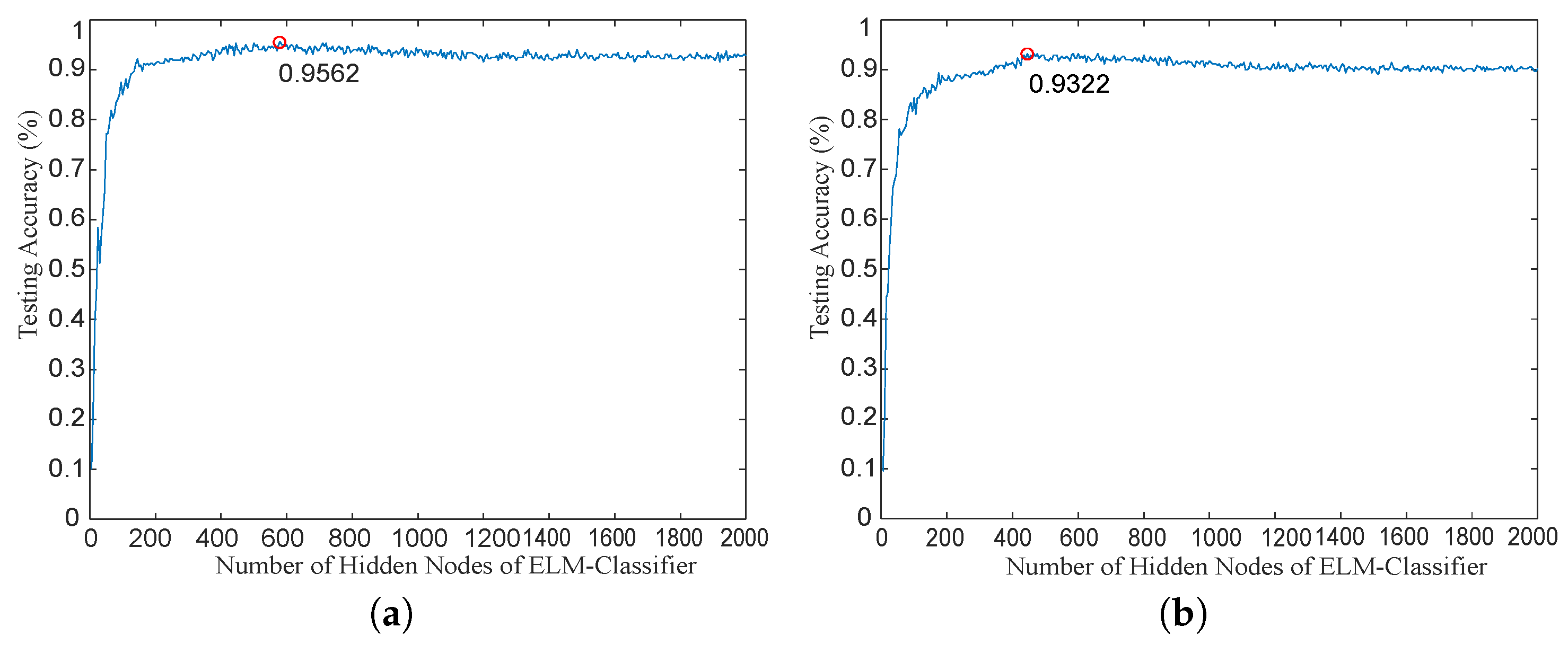As shown in Figure 7a,b,we set the number of hidden layer nodes $L=800$, when the number of hidden layer nodes l increase from 1 to 2000 at 10 interval, the largest accuracy is 95.62% at single fault condition and 93.22% simultaneous-fault condition, respectively. The optimal hidden layer nodes in the classifier is set as $l=600$.

As suggested in

Table 5. Evaluation of different combinations of methods using the optimal model parameters. Wavelet packet transform: WPT; time-domain statistical features: TDSF; kernel principal component analysis: KPCA; empirical mode decomposition: EMD.

Feature Extraction	Classifier	Accuracies for Test Case (%)
		Single-Fault	Simultaneous-Fault	Overall Fault
WPT+TDSF+KPCA	PNN	83.64	83.64	83.76
	RVM	82.99	74.64	81.21
	SVM	92.88	89.73	90.78
	ELM	91.29	89.72	90.89
EMD+TDSF	PNN	85.64	84.64	84.52
	RVM	83.99	77.64	83.21
	SVM	95.83	92.87	94.35
	ELM	96.20	92.44	94.32
LMD+TDSF	PNN	85.64	84.64	84.52
	RVM	83.99	77.64	83.21
	SVM	95.25	92.87	93.27
	ELM	95.83	93.04	94.44
ELM-AE	PNN	85.64	84.64	84.52
	RVM	83.99	77.64	83.21
	SVM	95.83	92.87	93.27
	ELM	95.62	93.22	94.42

, a total of 16 kinds of combinations of method are implemented to compare the generation performance. According to the feature extraction, this paper takes three kinds of methods as references. They are WPT+TDSF+KPCA combination, EMD+SVD combination and LMD+TDSF combination, respectively. This paper takes the Db4 (Daubechies) wavelet as the mother wavelet and sets the level of decomposition at the range from 3 to 5. The radial basis function (RBF) acts as kernel function for KPCA. In order to reduce the number of trials, the hyperparameter R of RBF based on $2^v$ is tried for v ranged from – 3 to 3. In the KPCA processing, this paper selects the polynomial kernel with $d=4$ and the RBF kernel with $R=2$. After dimension reduction, a total of 80 principal components are obtained. After feature extraction, the next step is to optimize parameters of classifiers. This paper takes four kinds of methods, namely PNN, RVM, SVM and ELM. As mentioned previously, probabilistic based classifiers have their own hyperparameters for tuning. PNN uses spread s and RVM employs width $\mathsf{\omega }$. In this case study, the value of s is set from 1 to 3 at an interval of 0.5, and the values of $\mathsf{\omega }$ is selected from 1 to 8 at an interval of 0.5. In order to find the optimal decision threshold, this paper sets the search region at the range from 0 to 1 at an interval of 0.01. For the configuration of ELM, this paper takes the sigmoid function as the activation function and sets the number of hidden modes l as 600 for a trial. According to the experimental results in Table 4, a total of 80 components are obtained from the feature extractor. It is clear that the accuracies with autoencoder are higher than those with WPT+TDSF+KPCA. The results can be explained because the ELM based autoencoder holds all information of the input data during the representational learning. However, KPCA tends to hold the important information and inevitably lose some unimportant information.

In order to compare the performances of classifiers, this paper sets the contrast experiments with the same ELM based autoencoder and different classifiers. As shown in Table 5, the number of hidden nodes L in autoencoder is 800, the last dimensions of training data $D_{\text{train}}$ and testing data $D_{\text{test}}$ are 1800×800 and 280×800, respectively. As suggested in Figure 7, this optimal value of l is 600. According to the experimental results not listed here, SVM employed polynomial kernel with $C=10$ and $d^{*}$ = 4 show the best accuracy.

Table 6. Evaluation of methods using ELM or SVM with ELM based autoencoder (Note: Dimension reduction from 20,480 to 80).

Feature Extraction	Fault Type	Accuracies for Test Case (%)		Time for Test Case (ms)
		SVM	ELM	SVM	ELM
ELM-AE	Single-fault	95.72 ± 2.25	95.62 ± 2.25	156 ± 0.9	18 ± 0.8
	Simultaneous-fault	92.98 ± 1.25	93.22 ± 3.25	158 ± 0.8	20 ± 0.5
	Overall fault	93.55 ± 3.15	94.42 ± 2.75	157 ± 0.4	20 ± 0.75

shows that the fault detection accuracy of ELM is similar to that of SVM, while the fault identification time of ELM and SVM take 20 ms and 157 ms respectively. The performance of ELM is much faster than SVM. Quick recognition is necessary for real-time fault diagnosis system. In actual WTGS application, the real-time fault diagnostic system is required to analyze signals for 24 hours per day. In terms of fault identification time, ELM is faster than SVM by 88.46%. The test results show that ELM and SVM have relatively high testing accuracies, but the advantage of ELM is embodied in testing time, which is very significant in real situation because a practical real-time WTGS diagnostic system will analyze more sensor signals than the two sensor signals used in this case study.

5. Conclusions

This paper proposes a new application of ELM to the real-time fault diagnostic system for rotating machinery. The framework is successfully applied on recognizing fault patterns coming from the WTGS. At the stage of data preprocessing, this study applies an ELM based autoencoder for data representational learning, which train a network of ELM slices to acquire the feature reconstruction, and then the ELM network generates a new low-dimensional representation. Unlike the well adopted data preprocessing methods using a combination of WPT, TDSF and KPCA, the proposed ELM based autoencoder could leverage the down-streamed classification accuracy in around 5%–10% for different corresponding classifiers. Compared with the widely-applied classifiers (e.g., SVM and RVM), ELM algorithm searches optimal solution from the feature space without any other constraints. Therefore, ELM network is superior to SVM at producing lightly higher diagnostic accuracy. Besides, ELM aims to generate a smaller weights and norms, and then gets a faster generalization performance than SVM. This study makes contributions at the following four aspects: (1) It is the first research to analyze the ELM based autoencoder as a tool for compressed representation; (2) It is the first application of ELM based autoencoder to the fault diagnosis for rotating machinery; (3) It is the original application of the proposed scheme to fault diagnosis of WTGS; (4) It is the first study to solely use ELM method as a combination of two different training processes in terms of regression and classification, to realize autoencoding and classification respectively. Since the proposed framework for fault diagnosis of wind turbine equipment is general, it is suitable to apply to other industrial problems.

References

1. Amirat, Y.; Benbouzid, M.E.H.; Al-Ahmar, E.; Bensaker, B.; Turri, S. A brief status on condition monitoring and fault diagnosis in wind energy conversion systems. Renew. Sustain. Energy Rev. 2009, 13, 2629–2636. [Google Scholar] [CrossRef] [Green Version]
2. Yin, S.; Luo, H.; Ding, S.X. Real-time implementation of fault-tolerant control systems with performance optimization. IEEE Trans. Ind. Electron. 2014, 61, 2402–2411. [Google Scholar] [CrossRef]
3. Wong, P.K.; Yang, Z.; Vong, C.M.; Zhong, J. Real-time fault diagnosis for gas turbine generator systems using extreme learning machine. Neurocomputing 2014, 128, 249–257. [Google Scholar] [CrossRef]
4. Yan, R.; Gao, R.X.; Chen, X. Wavelets for fault diagnosis of rotary machines: A review with applications. Signal Process. 2014, 96, 1–15. [Google Scholar] [CrossRef]
5. Fan, W.; Cai, G.; Zhu, Z.; Shen, C.; Huang, W.; Shang, L. Sparse representation of transients in wavelet basis and its application in gearbox fault feature extraction. Mech. Syst. Signal Process. 2015, 56, 230–245. [Google Scholar] [CrossRef]
6. Vincent, P.; Larochelle, H.; Bengio, Y.; Manzagol, P.A. Extracting and composing robust features with denoising autoencoders. In Proceedings of the 25th International Conference on Machine Learning, Helsinki, Finland, 5–9 July 2008; pp. 1096–1103.
7. Bianchi, D.; Mayrhofer, E.; Gröschl, M.; Betz, G.; Vernes, A. Wavelet packet transform for detection of single events in acoustic emission signals. Mech. Syst. Signal Process. 2015. [Google Scholar] [CrossRef]
8. Keskes, H.; Braham, A.; Lachiri, Z. Broken rotor bar diagnosis in induction machines through stationary wavelet packet transform and multiclass wavelet SVM. Electric Power Syst. Res. 2013, 97, 151–157. [Google Scholar] [CrossRef]
9. Li, N.; Zhou, R.; Hu, Q.; Liu, X. Mechanical fault diagnosis based on redundant second generation wavelet packet transform, neighborhood rough set and support vector machine. Mech. Syst. Signal Process. 2012, 28, 608–621. [Google Scholar] [CrossRef]
10. Wang, Y.; Xu, G.; Liang, L.; Jiang, K. Detection of weak transient signals based on wavelet packet transform and manifold learning for rolling element bearing fault diagnosis. Mech. Syst. Signal Process. 2015, 54, 259–276. [Google Scholar] [CrossRef]
11. Ebrahimi, F.; Setarehdan, S.K.; Ayala-Moyeda, J.; Nazeran, H. Automatic sleep staging using empirical mode decomposition, discrete wavelet transform, time-domain, and nonlinear dynamics features of heart rate variability signals. Comput. Methods Prog. Biomed. 2013, 112, 47–57. [Google Scholar] [CrossRef] [PubMed]
12. Khorshidtalab, A.; Salami, M.J.E.; Hamedi, M. Robust classification of motor imagery EEG signals using statistical time–domain features. Physiol. Meas. 2013, 34. [Google Scholar] [CrossRef] [PubMed]
13. Li, W.; Zhu, Z.; Jiang, F.; Zhou, G.; Chen, G. Fault diagnosis of rotating machinery with a novel statistical feature extraction and evaluation method. Mech. Syst. Signal Process. 2015, 50, 414–426. [Google Scholar] [CrossRef]
14. Allen, E.A.; Erhardt, E.B.; Wei, Y.; Eichele, T.; Calhoun, V.D. Capturing inter-subject variability with group independent component analysis of fMRI data: a simulation study. Neuroimage 2012, 59, 4141–4159. [Google Scholar] [CrossRef] [PubMed]
15. Du, K.L.; Swamy, M. Independent component analysis. In Neural Networks and Statistical Learning; Springer: New York, NY, USA, 2014; pp. 419–450. [Google Scholar]
16. Shlens, J. A tutorial on principal component analysis. Available online: http://arxiv.org/pdf/1404.1100v1.pdf (accessed on 7 April 2014).
17. Waldmann, I.P.; Tinetti, G.; Deroo, P.; Hollis, M.D.; Yurchenko, S.N.; Tennyson, J. Blind extraction of an exoplanetary spectrum through independent component analysis. Astrophys. J. 2013, 766. [Google Scholar] [CrossRef]
18. Mairal, J.; Bach, F.; Ponce, J. Task-driven dictionary learning. IEEE Trans. Pattern Anal. Mach. Intell. 2012, 34, 791–804. [Google Scholar] [CrossRef] [PubMed]
19. Lei, Y.; He, Z.; Zi, Y.; Chen, X. New clustering algorithm-based fault diagnosis using compensation distance evaluation technique. Mech. Syst. Signal Process. 2008, 22, 419–435. [Google Scholar] [CrossRef]
20. Bro, R.; Smilde, A.K. Principal component analysis. Anal. Methods 2014, 6, 2812–2831. [Google Scholar] [CrossRef]
21. Xanthopoulos, P.; Pardalos, P.M.; Trafalis, T.B. Principal component analysis. In Robust Data Mining; Springer: New York, NY, USA, 2013; pp. 21–26. [Google Scholar]
22. Hoque, M.S.; Mukit, M.; Bikas, M.; Naser, A. An implementation of intrusion detection system using genetic algorithm. Int. J. Netw. Secur. 2012, 4, 109–120. [Google Scholar]
23. Johnson, P.; Vandewater, L.; Wilson, W.; Maruff, P.; Savage, G.; Graham, P.; Macaulay, L.S.; Ellis, K.A.; Szoeke, C.; Martins, R.N. Genetic algorithm with logistic regression for prediction of progression to Alzheimer’s disease. BMC Bioinform. 2014, 15. [Google Scholar] [CrossRef] [PubMed]
24. Whitley, D. An executable model of a simple genetic algorithm. Found. Genet. Algorithms 2014, 2, 45–62. [Google Scholar]
25. Tang, J.; Deng, C.; Huang, G.B. Extreme Learning Machine for Multilayer Perceptron. IEEE Trans. Neural Netw. Learn. Syst. 2015, 27, 809–821. [Google Scholar] [CrossRef] [PubMed]
26. Hinton, G.E. A practical guide to training restricted boltzmann machines. In Neural Networks: Tricks of the Trade; Springer: Lake Tahoe, NV, USA, 2012; pp. 599–619. [Google Scholar]
27. Srivastava, N.; Salakhutdinov, R.R. Multimodal learning with deep boltzmann machines. In Advances in Neural Information Processing Systems; Springer: Lake Tahoe, NV, USA, 2012; pp. 2222–2230. [Google Scholar]
28. Fischer, A.; Igel, C. An introduction to restricted Boltzmann machines. In Progress in Pattern Recognition, Image Analysis, Computer Vision, and Applications; Springer: Buenos Aires, Argentina, 2012; pp. 14–36. [Google Scholar]
29. Yang, Z.; Wong, P.K.; Vong, C.M.; Zhong, J.; Liang, J. Simultaneous-fault diagnosis of gas turbine generator systems using a pairwise-coupled probabilistic classifier. Math. Probl. Eng. 2013, 2013. [Google Scholar] [CrossRef]
30. Vong, C.M.; Wong, P.K. Engine ignition signal diagnosis with wavelet packet transform and multi-class least squares support vector machines. Expert Syst. Appl. 2011, 38, 8563–8570. [Google Scholar] [CrossRef]
31. Abbasion, S.; Rafsanjani, A.; Farshidianfar, A.; Irani, N. Rolling element bearings multi-fault classification based on the wavelet denoising and support vector machine. Mech. Syst. Signal Process. 2007, 21, 2933–2945. [Google Scholar] [CrossRef]
32. Widodo, A.; Yang, B.S. Application of nonlinear feature extraction and support vector machines for fault diagnosis of induction motors. Expert Syst. Appl. 2007, 33, 241–250. [Google Scholar] [CrossRef]
33. Sankari, Z.; Adeli, H. Probabilistic neural networks for diagnosis of Alzheimer’s disease using conventional and wavelet coherence. J. Neurosci. Methods 2011, 197, 165–170. [Google Scholar] [CrossRef] [PubMed]
34. Othman, M.F.; Basri, M.A.M. Probabilistic neural network for brain tumor classification. In Proceedings of the 2011 Second International Conference on Intelligent Systems, Modelling and Simulation (ISMS), Kuala Lumpur, Malaysia, 25–27 January 2011; pp. 136–138.
35. Huang, G.B.; Zhou, H.; Ding, X.; Zhang, R. Extreme learning machine for regression and multiclass classification. IEEE Trans. Syst. Man Cybern. Part B Cybern. 2012, 42, 513–529. [Google Scholar] [CrossRef] [PubMed]
36. Huang, G.B.; Ding, X.; Zhou, H. Optimization method based extreme learning machine for classification. Neurocomputing 2010, 74, 155–163. [Google Scholar] [CrossRef]
37. Huang, G.B.; Zhu, Q.Y.; Siew, C.K. Extreme learning machine: theory and applications. Neurocomputing 2006, 70, 489–501. [Google Scholar] [CrossRef]
38. Huang, G.B. What are Extreme Learning Machines? Filling the Gap Between Frank Rosenblatt’s Dream and John von Neumann’s Puzzle. Cognit. Comput. 2015, 7, 263–278. [Google Scholar] [CrossRef]
39. Wong, P.K.; Wong, K.I.; Vong, C.M.; Cheung, C.S. Modeling and optimization of biodiesel engine performance using kernel-based extreme learning machine and cuckoo search. Renew. Energy 2015, 74, 640–647. [Google Scholar] [CrossRef]
40. Luo, J.; Vong, C.M.; Wong, P.K. Sparse bayesian extreme learning machine for multi-classification. IEEE Trans. Neural Netw. Learn. Syst. 2014, 25, 836–843. [Google Scholar] [PubMed]
41. Cambria, E.; Huang, G.B.; Kasun, L.L.C.; Zhou, H.; Vong, C.M.; Lin, J.; Yin, J.; Cai, Z.; Liu, Q.; Li, K.; et al. Extreme learning machines [trends and controversies]. IEEE Intell. Syst. 2013, 28, 30–59. [Google Scholar] [CrossRef]
42. Widrow, B.; Greenblatt, A.; Kim, Y.; Park, D. The No-Prop algorithm: A new learning algorithm for multilayer neural networks. Neural Netw. 2013, 37, 182–188. [Google Scholar] [CrossRef] [PubMed]
43. Bartlett, P.L. The Sample Complexity of Pattern Classification with Neural Networks: The Size of the Weights is More Important than the Size of the Network. IEEE Trans. Inf. Theory 1998, 44, 525–536. [Google Scholar] [CrossRef] [Green Version]
Figure 1. Diagram and fault simulator for wind turbine generator system (WTGS). (a) The diagram of WTGS; (b) the simulation platform of WTGS.
Energies 09 00379 g001
Figure 2. The proposed fault diagnostic framework using an extreme learning machine (ELM) based autoencoder and classifier. (a) ELM-autoencoder (AE) output weights β 1 with respect to input data x are the 1st layer weights of Multilayered (ML)-ELM; (b) The output weights β i + 1 of ELM-AE, with respect to i t h hidden layer output hi of ML-ELM are the i + 1 t h layer weights of Multilayered-ELM; (c) The Multilayered-ELM output layer weights are calculated using regularized least squares.
Energies 09 00379 g002
Figure 3. ELM orthogonal random feature mapping.
Energies 09 00379 g003
Figure 4. The proposed real-time fault diagnostic scheme for WTGS.
Energies 09 00379 g004
Figure 5. Singular Component Failure in WTGS. (a) Gear tooth broken fault; (b) gear crack fault; (c) chipped tooth fault; (d) mechanical misalignment fault; (e) wear of cage and rolling elements of bearing; (f) Unbalance.
Energies 09 00379 g005
Figure 6. Sample normalized simultaneous-fault patterns of WTGS. (a) Gear tooth broken and chipped tooth; (b) chipped tooth and wear of outer race of bearing; (c) gear tooth broken and wear of cage and rolling elements of bearing; (d) gear tooth broken and wear of cage and rolling elements of bearing and wear of outer race of bearing.
Energies 09 00379 g006
Figure 7. Testing accuracy in l subspace for the multi-layered ELM when L = 800. (a) Testing accuracy of single-fault; (b) Testing accuracy of simultaneous-fault.
Energies 09 00379 g007