The Impact of Renewable Energy Policies on the Adoption of Anaerobic Digesters with Farm-Fed Wastes in Great Britain

Abstract

This paper explores the effects of the feed-in tariff (FiT) and renewable heat incentive (RHI) schemes on the adoption of anaerobic digesters (AD), and the potential energy generation from farm-fed wastes in Great Britain. This paper adopts a linear programming model, developed in the International Energy Agency (IEA) TIMES platform, aiming to quantify the degree of adoption of AD and the type of energy generation technologies that can be driven by digester biogas to reduce farm energy costs. The results show that the adoption of AD is cost-beneficial for all farms, but different rates of the FiT and RHI schemes will influence the competitiveness between the implementation of combined heat and power (CHP) systems and the utilisation of biogas to only generate heat. The choice of technology is further dependent on the electricity/heat use ratio of the farms and the energy content of the feedstock. The results show that pig farms will more readily adopt CHP, because of its relatively higher electricity-to-heat use ratio, compared to other types of farms, which will favour biogas boilers.

1. Introduction

1.1. Context

The Food and Agriculture Organisation (FAO) of the United Nations has expressed concerns over global food security particularly due to the projected increase in population, urbanisation, diet diversification and climate change. These concerns arise mainly from issues surrounding the use of available resources to satisfy increasing food demand, the high dependency of food production on depleting and price-inflated fossil-fuels, and the associated effects on the climate [1]. Additionally, the UK Climate Change Act 2008 has set an ambitious target to reduce the greenhouse gas (GHG) emissions by 80% in 2050, as well as generating 15% of the energy from renewable sources by 2020 [2], compared to 1990 levels. In line with both food security concerns and the UK GHG emissions reduction targets, agriculture represents a significant sector that needs attention in order to address future food and energy issues. In 2011, the UK agri-food sector was found to contribute about 32% to the overall GHG emissions generated by the country, with agriculture representing the largest share with approximately 30% of the total agri-food sector emissions [3,4]. In order to tackle the 9% agricultural GHG emissions share of the total UK GHG emissions, the UK has identified solutions revolving around enhancing livestock efficiency, improving fertiliser use and manure management, and altering demand for livestock products [5]. Currently, with respect to the total agriculture emissions, it is estimated that fertiliser use contributes 53%, enteric fermentation 30%, combustion processes 9%, and manure management 8% [5]. With regards to livestock management and enteric fermentation, principal approaches to reducing emissions involve selective breeding, improved livestock management and modifying livestock diet. Additionally, it was identified that anaerobic digestion (AD) can make a significant contribution to the simultaneous reduction of emissions from fertiliser use, manure management and combustion [6]. AD refers to the breakdown of biodegradable organic material by bacteria in the absence of oxygen, to produce biogas and a nutrient-rich digestate/fertiliser. By using the large amount of manure and slurries generated by farms, which are currently stored and/or spread on lands, in AD plants to produce biogas and biofertiliser, would replace fossil fuels and replace inorganic fertilisers with AD digestate. AD would also benefit farmers with reduced costs and additional income-generation (from the export of energy or fertiliser), employment creation, odour reduction and control of diffuse pollution through improved waste management. Furthermore, compared with other renewable energy technologies such as wind, solar and tidal, AD can provide a continuous, controllable and scalable energy generation, adaptable to different organic feedstocks [7].

1.2. State of Application of Anaerobic Digestionin British Farms

In 2014, the number of AD plants in Great Britain (GB) reached 147 [8]. This number is however small compared to other countries such as Germany with 7850 systems in 2013 [9] or Sweden with 173 plants in 2011 [6]. The distribution of AD plants is shown in Figure 1, where: (i) commercial plants refer to sites that import feedstock, set up as the third party contracts that mainly use food waste, crop silage and municipal solid wastes; (ii) industrial plants are sites that use effluents and industrial waste as feedstock; (iii) integrated plants employ different non-source segregated feedstocks; and (iv) on-farm plants process farm-fed slurries, manures, crops or crop residues produced on farm. For the purpose of this study, the emphasis will be on the “on-farm” plants using principally manures and slurries. Waste and Resources Action Programme (WRAP) estimates that there is currently 67 on-farm AD plants, with 47 plants employing some form of manures/slurries and 36 sites using manure as feedstock for CHP units, with the rest having boilers [8]. The aim of implementing and promoting AD plants by the government is to mainly promote the generation of both heat and electricity from the produced biogas, and/or supplement the national electricity and gas grid through the export of electricity and bio-methane from AD.

As previously mentioned, the uptake of such AD plants has been slow compared to other European countries. A study by Tranter et al. [10] found that most UK farmers consider maximising profits as their primary focus, prior to reducing pollution or carbon footprint. The study showed that farmers defined the adoption barriers for AD, in decreasing importance, to be: high capital cost; low return on investment; difficulty in obtaining planning permission; and a lack of adequate information for decision-making. In the majority of cases, reference to AD plant implies both anaerobic digestion for the production of biogas and the combustion of biogas in a combined heat and power (CHP) plant for the production of both heat and electricity. In most cases, the capital cost of establishing just the anaerobic digester represents approximately 35%–40% of the total capital cost of the plant including the electricity generation facility [11]. The electricity generation facility requiring a CHP unit, may lead to significant extra capital and maintenance costs, and additional engineering system complexity compared to plant producing only heat [12].From the surveys carried out by Tranter et al. [10], it is apparent that farmers understand the benefits of an anaerobic digester in terms of biogas and bio-fertiliser production, but have difficulties in appreciating the economics of establishing and operating a combined AD and CHP system.

1.3. UK Government Incentives for Anaerobic Digestion

In order to promote the adoption of AD systems and the generation of electricity from the biogas produced, the UK government has devised two main mechanisms: the renewable heat incentive (RHI) and the feed-in tariff (FiT). The FiT, introduced in 2010, is an incentive given to small scale renewable electricity generation technologies, including electricity generated from AD, to encourage local electricity generation. The RHI, introduced in 2011, incentivises the generation of heat or biomethane using renewable sources. It applies to biomass combustion, biogas combustion, heat pumps, solar collectors and geothermal energy. The durations of the RHI and the FiT schemes are for 20 years, and new entrants are expected to be accepted until 2021. The subsidy rates for AD are shown in Figure 2a,b below, obtained from references [13,14].

The value of the monetary incentives varies with the retail price index of the economy, and the rates for new applicants subjected to a degression factor (see Section 2.4), to account for the decrease in price of renewable energy technologies with time. It is also important to note that these incentives are quantity-based, requiring the farmer to first find the capital to invest, before they can see a return on their investment, based on the performance of their energy generation system. Figure 2a,b shows that the rates for AD have been decreasing over the years due to reduction in costs and the degression rates applied by the UK government. These reductions are accounted for in this study, and the rates beyond 2020 are assumed constant.

In addition to monetary incentives, the government introduced a quality protocol in 2010, whereby the digestate produced using farm-feedstocks (such as manures, slurries and crops) is not considered as waste, provided adequate storage and use practices are maintained, and therefore does not have to undergo waste management operations before being used as fertiliser [15,16].

1.4. Objective

The aim of this paper is to determine the extent to which the monetary based government incentives will have an influence on the adoption rate of AD systems, and corresponding energy generation technologies employing AD biogas. The study employs a macroeconomic approach to modelling AD plants in a whole-farm context, in order to determine the plausible contribution of AD plants to the energy consumption of farms towards 2050. The study does not aim to determine ways of optimising current technologies, but rather to examine the optimisation of available technology mix towards 2050, and identify possible drawbacks of energy policies to limiting the implementation of AD and energy generation systems on farms.

2. Methodology

2.1. Review of Existing Modelling Approach

In 2007, Mistry and Smith [17] studied, on behalf of the UK Department of Environment, Food and Rural Affairs (DEFRA), the economics of AD-CHP plants in the UK using livestock and other wastes as feedstock. The model employed the internal rate of return (IRR) as an indicator of the efficiency of the investment, whereby the project is valuable if the return is greater than the plant’s capital cost. The model used simple capital cost correlations based on a limited quantity of available data and different subsidy rate scenarios, and concluded that currently only 3.5% of UK dairy livestock would be financially benefit from using on-farm AD-CHP plants. In order to increase this proportion to a potential 18% of dairy farms, a significant reduction of capital costs or a doubling of the FiT rate would be required. Similarly, Dolan et al. [18] employed an IRR approach to quantify the economic viability of general wet mesophilic AD-CHP plants in the UK using source segregated organic waste, whereby the conclusion was that under the government’s energy incentives, selling excess heat and electricity from AD-CHP plants doubles the IRR, compared to only injecting Biomethane to the grid. Zglobisz et al. [19] also employed the IRR approach to examine the impact of UK policies on the deployment of AD plants using food waste as the primary feedstock. Their model showed that doubling the electricity incentive subsidy rates, in conjunction with RHI, would significantly improve the IRR of AD-CHP plants.

Various case studies (see [12]) have shown that the implementation of AD plants in farms varies with respect to the capital cost, types of feedstock, biogas use and farm activities. Furthermore, the small number of on-farm AD plants and the lack of empirical data on such plants pose uncertainties on the viability of AD plants on farms. In this regard, the National Non-Food Crops Centre (NNFCC) AD calculator evaluation tool [20] has been developed to aid potential operators of AD-CHP plants to assess the viability and potential returns on their investment based on different FiT and RHI rates. Previous studies, although not extensive in numbers, have focused mainly on using IRR to determine the economic viability of AD plants in the UK, considering the plant as a stand-alone investment. However as alluded in Section 1.2, farms have complex structures. Farmers are more interested in maximising returns for the farm as a whole, as opposed to only considering the IRR of AD-CHP plants when deciding to invest in such plants. As such, because the FiT and RHI schemes promote energy generation from AD plants, farms will also assess the competitiveness and return from different energy generation technologies as opposed to solely CHP, in an attempt to minimise overall farm costs.

2.2. Modelling Approach

This study employs the linear programming technique to analyse the viability of AD in Great Britain (GB) farms. Linear programming techniques have been widely used in modelling farm management decisions such as: [7,21,22,23], where the objective function—total costs or net profit margins—can either be minimised or maximised, subject to technical, economic, environmental and resource constraints. The IEA-ETSAP (Energy Technology Systems Analysis Program) TIMES (The Integrated MARKAL-EFOM System) model generator is used here to link the technologies, energy and cost structures of farms in a partial equilibrium model, and together with a technology-rich foundation, it allows the estimation of energy dynamics over a long-term horizon [24]. TIMES uses a linear optimisation objective function which determines the least-cost pathway by minimising the total discounted system costs in order to satisfy the farm’s energy demands, subject to technical, economic, environmental and resource constraints. Through the use of a partial equilibrium solution strategy, the model does not provide feedback on other sector changes, and assumes perfect foresight as decisions are made with full knowledge of future policy, technical, economic developments and available resources [25].

The linkages between the inputs and outputs for each technology and the overall energy structure in GB farms are shown in Figure 3. The analysis aims to encompass the onsite farm energy in its entirety, considering the electricity, fuel and fertiliser demands. Fertiliser demand is considered as the digestate produced from AD can be used as biofertiliser, thus representing an additional opportunity benefit from AD, which incentivises the implementation of AD systems on farms. Figure 3 shows that the energy technologies considered: gas/biogas boilers, biomass boilers, CHP system, AD, grid supply of electricity, purchased fuel, and purchased fertiliser. The schematic shows that in order to satisfy its energy demand and benefit from government incentives, farms can employ: (i) the biogas from AD via a CHP to produce electricity and heat, and benefit from both the FiT and RHI; (ii) export the electricity and benefit from additional FiT export revenues; (iii) the biogas in a boiler and benefit from RHI; (iv) purify and export biogas (converted to biomethane) to the grid, and benefit from the RHI; or (v) avoid the AD and dry the biomass, to be used in a biomass boiler. A further avenue for income would be to sell the biofertiliser, which is not considered in this study, as there are currently no government incentives for biofertiliser export, whereby farms tend to use all biofertiliser produced [16]. The simultaneous consideration of these various technologies allows the determination of the real performance of the energy incentives, as it accounts for the price competitiveness of other technologies compared to AD or CHP, as opposed to using the internal IRR which considers the technologies in isolation. Thus, this methodology provides an optimal solution in terms of the combination/interaction of different technologies. The base year for the simulation is 2013.

2.3. Farm Characteristics

Table 1. AD feedstock characteristics from animal manure/slurry [27].

Animals	Manure/Slurry Yield (t/Month)	Housing Occupancy (%)	Biogas Yield (m3/t Feedstock)
1 Calf	0.21	60%	25
1 Dairy cow	1.31	100%	25
1 Beef	0.90	60%	35
1 Bull	0.78	50%	25
1 Lamb	0.05	50%	35
1 Sheep	0.13	10%	35
1 Goat	0.10	10%	35
1 Weaner pig	0.04	71%	44
1 Grower pig	0.14	88%	44
1 Finisher pig	0.20	86%	44
1 Sow	0.33	100%	44
1 Breeding boar	0.21	100%	44
1000 Young chickens (<25 weeks)	1.10	89%	80
1000 Full grown chicken/broilers	3.50	97%	80
1000 Turkey	3.75	89%	80
1000 Ducks	2.50	83%	80

shows the characteristics of manure/slurry produced by different animals, as well as the housing occupancy period used in the model [2], whilst

Table 2. Biogas Yield from crop feedstocks to AD [26]. NPK: nitrogen, phosphorus and potassium.

Crops	Average NPK Requirements (kg/ha)	Biogas Yield (m3/t Feedstock)
Winter wheat	113.3	185.0
Barley	106.7	505.5
Other cereals	106.7	250.0
Oilseed rape	96.7	340.0
Peas and beans	30.0	390.0
Potatoes	206.7	338.0
Sugar beet	75.0	308.5
Other crops including horticultural crops	110.0	242.0
Fallow and arable fodder crops	111.7	213.0

shows the biogas yield from crop feedstock [26]. For the purpose of this study, as the nutrient content of AD digestate typically varies in the range of nitrogen-N (2.3–1.2 kg of nutrient/tonne of digestate), phosphorus-P (0.2–1.5 kg of nutrient/tonne of digestate) and potassium-K (1.3–5.2 kg of nutrient/tonne of digestate) according to feedstock [15], which is within the range required by the crops defined in Table 2 [10], the AD digestate is assumed to directly replace conventional inorganic fertilisers [7]. In the UK, animal farms are generally classified as dairy, lowland, less-favourable area (LFA), specialist pig and specialist poultry farms [27], where, in all cases, the animals being reared and crops grown vary, as shown in

Table 3. Annual dairy farm input and output characteristics [27]. LPG: liquefied petroleum gas.

Commodity	Low-Performing Farms	Medium-Performing Farms	High-Performing Farms
Crops grown (with respect to total farm area by performance band)
Winter wheat	6%	7%	5%
Winter barley	2%	1%	1%
Spring barley	4%	3%	4%
Other cereals	0%	1%	0%
Oilseed rape	2%	0%	1%
Fallow and arable fodder crops	16%	17%	12%
Total utilised farm area (ha)	127.4	151.2	156.9
Animals produced (with respect to total farm animals by performance band)
Dairy cows	35%	44%	40%
Beef cows	0%	0%	0%
Calves and other cattle	32%	39%	38%
Ewes	15%	8%	4%
Sheeps	16%	8%	9%
Pigs	0%	1%	9%
Poultry	2%	0%	0%
Total animals per farm (units)	347	397	479
Energy used (GJ/animal) (by performance band)
Electricity	3.13	3.85	3.80
Kerosene	0.04	0.05	0.05
LPG	0.02	0.02	0.02
Natural gas	0.00	0.00	0.00
Other fuels (fuel oil, coal, gas oil)	0.20	0.24	0.24
Electricity to heat use ratio	12.0	12.4	12.3

,

Table 4. Annual Lowland farm input and output characteristics [27].

Commodity	Low-Performing Farms	Medium-Performing Farms	High-Performing Farms
Crops grown (with respect to total farm area by performance band)
Winter wheat	0%	1%	2%
Winter barley	2%	1%	1%
Spring barley	1%	3%	2%
Other cereals	1%	0%	1%
Oilseed rape	0%	0%	0%
Fallow andarable fodder crops	2%	3%	4%
Total utilised farm area (ha)	58.7	92.1	134.8
Animals produced (with respect to total farm animals by performance band)
Dairy cows	0%	0%	0%
Beef cows	6%	5%	4%
Calves and other cattle	13%	19%	19%
Ewes	39%	34%	38%
Sheeps	38%	38%	38%
Pigs	1%	0%	0%
Poultry	2%	2%	1%
Total animals per farm (units)	284	425	589
Energy used (GJ/animal) (by performance band)
Electricity	0.16	0.18	0.19
Kerosene	0.05	0.06	0.06
LPG	0.00	0.01	0.01
Natural gas	0.00	0.00	0.00
Other Fuels (fuel oil, coal, gas oil)	0.01	0.01	0.01
Electricity to heat use ratio	2.7	2.3	2.4

,

Table 5. Annual less-favourable area (LFA) farm input and output characteristics [27].

Commodity	Low-Performing Farms	Medium-Performing Farms	High-Performing Farms
Crops grown (with respect to total farm area by performance band)
Winter wheat	0%	0%	0%
Winter barley	0%	0%	0%
Spring barley	0%	1%	0%
Other cereals	0%	0%	0%
Oilseed rape	0%	0%	0%
Fallow and arable fodder crops	0%	0%	0%
Total utilised farm area (ha)	73.2	138.2	223.5
Animals produced (with respect to total farm animals by performance band)
Dairy cows	0%	0%	0%
Beef cows	5%	3%	3%
Calves and other cattle	10%	7%	7%
Ewes	46%	46%	48%
Sheeps	38%	44%	42%
Pigs	0%	0%	0%
Poultry	0%	0%	0%
Total animals per farm (units)	418	877	939
Energy used (GJ/animal) (by performance band)
Electricity	0.05	0.05	0.07
Kerosene	0.02	0.02	0.02
LPG	0.00	0.00	0.00
Natural Gas	0.00	0.00	0.00
Other fuels (fuel oil, coal, gas oil)	0.00	0.00	0.00
Electricity to heat use ratio	2.5	2.5	3.5

,

Table 6. Annual specialist pig farm input and output characteristics [27].

Commodity	Medium-Performing Farms	High-Performing Farms
Crops grown (with respect to total farm area by performance band)
Winter wheat	19%	10%
Winter barley	7%	3%
Spring barley	9%	4%
Other cereals	4%	0%
Oilseed rape	1%	7%
Fallow and arable fodder crops	9%	34%
Total utilised farm area (ha)	38.65	115.06
Animals produced (with respect to total farm animals by performance band)
Dairy cows	0%	0%
Beef cows	0%	0%
Calves and other cattle	0%	0%
Ewes	1%	0%
Sheeps	1%	0%
Sows	7%	7%
Other pigs	87%	93%
Poultry	3%	0%
Total animals per farm (units)	1996	7360
Energy used (GJ/animal) (by performance band)
Electricity	1.23	1.31
Kerosene	0.00	0.00
LPG	0.00	0.00
Natural Gas	0.00	0.00
Other Fuels (fuel oil, coal, gas oil)	0.01	0.01
Electricity to heat use ratio	123.0	131.0

and

Table 7. Annual specialist poultry farm input and output characteristics [27].

Commodity	Low-Performing Farms	Medium-Performing Farms	High-Performing Farms
Crops grown (with respect to total farm area by performance band)
Winter wheat	10%	9%	26%
Winter barley	0%	4%	3%
Spring barley	6%	7%	2%
Other cereals	0%	6%	0%
Oilseed rape	11%	5%	12%
Fallow and arable fodder crops	3%	2%	8%
Total utilised farm area (ha)	19.71	40.70	66.15
Animals produced (with respect to total farm animals by performance band)
Dairy cows	0%	0%	0%
Beef cows	0%	0%	0%
Calves and other cattle	0%	0%	0%
Ewes	0%	0%	0%
Sheeps	0%	0%	0%
Pigs	0%	0%	0%
Hens and pullets in lay	71%	24%	5%
Poultry	28%	76%	95%
Total animals per farm (units)	13,496	67,094	129,605
Energy used (GJ/animal) (by performance band)
Electricity	0.016	0.003	0.002
Kerosene	0.005	0.001	0.001
LPG	0.003	0.000	0.000
Natural gas	0.000	0.000	0.000
Other Fuels (fuel oil, coal, gas oil)	0.0002	0.000	0.000
Electricity to heat use ratio	2.0	3.0	2.0

. For reporting purposes of the national farm accounts, these farms are further sub-classified according to their performance levels (low, medium and high) according to [27].

The quantity of feedstock used as input to AD systems are evaluated from the data shown in Table 3, Table 4, Table 5, Table 6 and Table 7, including the fact that in order for farms to maximise the energy generation potential of AD systems with manure/slurries, a minimum amount of 30% crop material is required [28]. It should be noted that the fuels considered in Table 3, Table 4, Table 5, Table 6 and Table 7 refer only to the fuels which generate useful heat for farms, as opposed to fuels in mobile machinery.

2.3.1. Dairy Farms

Dairy farms tend to consist of a majority of maturing cows and calves which are housed indoors approximately 60% of the time, and lactating cows which are fully housed all year round (as shown in Table 1). The model therefore accounts for the generation of manure/slurries at a rate of 1.51 t/year, 6.5 t/year, 4.7 t/year and 15.7 t/year per calf, beef, bull and lactating cows, respectively. Furthermore, dairy farms also tend to comprise of other animals and crops, as well as different energy consumption levels for different performance bands, as shown in Table 3.

The AD capacity in 2013 has been estimated to be a total of 9 units in dairy farms with a total capacity of 3242 tonnes, 12,544 tonnes and 171,623 tonnes for low, medium and high performance farms, respectively. Additionally, the associated total installed CHP capacities were found to be 15 kWe (total of 3 units), 125 kWe (total of 3 units) and 3920 kWe (total of 3 units), with respect to each farm performance band [8].

2.3.2. Grazing Livestock (Lowlands) Farms

Grazing livestock lowland farms account for approximately 10% of farmed land in England and generates the lowest income per farm [29]. Such farms refer to farms with more than two-thirds of their standard output are cattle and sheep (excluding holdings classified as dairy) and with less than 50% of their area as less favoured area [29] as defined by EC1257/1999. The inputs and outputs of standard Lowland farms, divided by performance band, is shown in Table 4.

In 2013, there was an estimated 7 AD in Grazing Lowland Farms with a total capacity of 1682 tonnes, 3633 tonnes and 37,890 tonnes for low, medium and high performing farms, respectively. The associated CHP capacity was estimated to be 4 kWe (total of 1 unit), 29 kWe (total of 2 units) and 1206 kWe (total of 4 units), for the respective performance bands [8]. The total energy consumption on the farm is lower than other non-grazing farms, as most energy is used in the form of red diesel used in tractors.

2.3.3. Grazing Livestock less Favoured Area Farms

LFA grazing livestock farms are defined by the European Council regulation EC 1257/1999 as farms located in mountain areas, areas in danger of abandonment of agricultural land-use and where the conservation of the countryside is necessary, and areas affected by specific handicaps (such as continuing agriculture in order to protect coastline) [30]. LFA farms also benefit from low profitability and have undertaken diversification activity to increase income [29]. The inputs and outputs of standard LFA farms, divided by performance band, is shown in Table 5.

In 2013, there was an estimated 7 Anaerobic digesters in Grazing LFA Farms with a total capacity of 1723 tonnes, 3461 tonnes and 40,610 tonnes for low, medium and high performing farms, respectively. The associated CHP capacity was estimated to be 4 kWe (total of 1 unit), 27 kWe (total of 2 units) and 1294 kWe (total of 4 units), for the respective performance bands [8].

2.3.4. Specialist Pig Farms

Although pig farms tend to mainly produce pigs, the outputs are not exclusively pigs, especially for smaller scale farms. As shown in Table 1, pigs are housed for 71%–100% of the year depending on the age of the animal, and hence the energy consumed by such farms tends to be higher compared to the grazing farms due to building conditioning requirements. The input and output characteristics of specialist pig farms can be found in Table 6 (note that DEFRA does not account for low-performing pig farms [27]).

In 2013, AD plants were estimated at a capacity of 70,815 tonnes, only for high performing farms, with an associated CHP capacity of 3400 kWe (total of 4 units) [8].

2.3.5. Specialist Poultry Farms

In poultry farms, the animals are housed for long periods during the year typically 97% (refer to Table 1—of which approximately 94% of poultry production consists of broiler chickens [31]). Hence, similar to pig farms, the energy consumed by the conditioning of poultry enclosures, accounts for a large ratio of energy use. The input and output characteristics of specialist poultry farms can be found in Table 7.

In 2013, it was estimated that only medium and high performance farms had adopted AD plants: a total capacity of 16,700 tonnes and 14,200 tonnes for medium and high performance farms, respectively, with an associated total CHP capacity of 750 kWe and 730 kWe, respectively [31].

2.4. Technology Specifications

The technologies considered in this study, depicted in Figure 3, focus on the generation of heat and/or electricity. The aim of adopting these technologies is to primarily produce useful heat/electricity for usage on farms, and subsequently export any excesses.

Table 8. Characteristics of technologies used in this study [7,12,26].

Technology	Size	Capital Costs	Operating and Maintenance Costs	Lifetime
AD + CHP	50 kWe	7144.00 £/kWe	607.00 £/kWe	25 years
	100 kWe	6728.00 £/kWe	571.00 £/kWe	25 years
	200 kWe	5967.00 £/kWe	507.00 £/kWe	25 years
	300 kWe	5292.00 £/kWe	449.00 £/kWe	25 years
	400 kWe	4694.00 £/kWe	398.00 £/kWe	25 years
	500 kWe	4163.00 £/kWe	353.00 £/kWe	25 years
	1000 kWe	2285.00 £/kWe	194.00 £/kWe	25 years
AD	All	17.13 £/ton	1.20 £/ton	15 years
Fuel-oil/Gas oil boiler	All	120.00 £/kWth	3.60 £/kWth	25 years
Biomass boiler	All	190.00 £/kWth	5.70 £/kWth	25 years
Biogas boiler	All	40.00 £/kWth	1.20 £/kWth	25 years
Biomass dryer	All	40.33 £/ton	1.18 £/ton	25 years
Storage tank	All	6.10 £/ton	0.50 £/ton	25 years
Export of biogas (grid is currently not adequate)	-	-	-	-

shows the cost characteristics of technologies supplied to the model, in order to produce the optimal least-cost pathway. It should be noted that this study does not intend to generate specific primary technological data for the different technologies, but rather, it has extensively surveyed academic, grey and industry literature to assign realistic values to the energy and cost performance of each technology.

The “AD only” costs comprise of the cost of the AD plant and storage unit required for the plant, estimated at around 35% of the total average “AD + CHP” plant [11]. Furthermore, with regards to UK farms, 24% of the system capacity are thermophilic, whilst 75% are mesophilic [16]. The digestate production is estimated at 85% of feedstock mass [16] and the amount of biogas is obtained from Table 1, according to the combination of feedstock used. Mesophilic AD, operating at lower temperatures was estimated to consume 0.01% and 7% of heat and electricity, respectively, relative to the amount of embedded energy in the produced biogas [32], whilst thermophilic AD was estimated to consume 25% and 4% of heat and electricity respectively, relative to the amount of embedded energy in the produced biogas [32]. The “AD + CHP” costs consist of the total cost to construct and operate the AD plant, the CHP system and the feedstock storage unit. These costs have been determined from information derived from references [7,8,12]. The reduction in unit price for increasing sizes, shown in Table 8, is due the reduction in CHP costs because of economies of scale, calculated linearly according to the electricity capacity of the CHP unit. The overall efficiency of the CHP unit is 75%, with a heat-to-power ratio of 1.3:1 [32], based on the commonly used reciprocating CHP type [33].The boilers described in Table 8 were assigned an efficiency of 80%, as per the suggestion of the Carbon trust [34]. The storage tanks were assumed to have no leakage. As the costs of technologies are expected to reduce with time, a degression rate of 15% was assigned to the capital costs of boilers [35] and 10% to AD [36], whilst the generic baseline UK degression rate of 5% was assigned to all other technologies [37].

Figure 4 shows the energy and fertiliser prices used in the model. It should be noted that fuel here refers to an average of kerosene and gas oil, which are most commonly used in farms—natural gas is not employed (as shown in Table 3, Table 4, Table 5, Table 6 and Table 7) due to farms being generally situated away from the gas grid. Projections in energy prices were obtained from data considering future economic growth, population and employment assumptions from the UK Department of Energy and Climate Change (DECC) [38]. However, because these projections are only available until 2035, Figure 4 also shows different extrapolations of possible changes in price after 2035 which are investigated in this study. Fuel prices have been linearly extrapolated following the clear trend prior to 2035, whilst the electricity prices also assumed to an increasing trend—as suggested by the UK Department for Business, Energy and Industrial Strategy (BEIS), the new entity replacing the UK DECC—due to the projected investment in more expensive nuclear and renewable technologies [38]. Fertiliser prices are projected from data obtained from the World Bank price forecasts [39]. Fertiliser prices are an average of nitrogen, potash and phosphate and as the World Bank only projects until a limited period (until 2025), the fertiliser prices until 2050 are extrapolated using the clear trend prior to the final data-year.

Figure 5 shows the projected quantities of local animal production used in this study, obtained from the FAPRI-UK project [40]. The FAPRI project considers the effect of the Common Agricultural Policy (CAP) in the EU in its projection of future animal production in GB. This report [40] however only provides projections until 2021, whereby for the purpose of this study, these projections were extrapolated according to the population growth rate until 2050. This embeds the assumption that the ratio of local production to imports (mainly European imports) of animals is maintained at year-2021 levels for the entire simulation horizon, and that meat consumption per capita will also stay constant at 2021 levels. Referring to Figure 5, it can be seen that production output from dairy farms stays relatively constant over the time-horizon, whilst the other farms increases in output. Furthermore, it was also observed that poultry and pig production increased by the highest percentages, 11.5% and 12%, respectively, over the time-horizon. Note that the relative quantities and type of animals are assumed constant over the time-horizon as described in Table 3, Table 4, Table 5, Table 6 and Table 7.

3. Results

The adoption rate of AD in different animal farms with respect to different FiT and RHI rates is quantified by the amount of biogas generated and consumed on the farms, while the self-sufficiency rate is portrayed by the reduction in grid electricity and fuel consumed by the farms. The results are portrayed according to the variations of the FiT and RHI Tariffs rates, with respect to the base rates. The base cases for all farm types refer to the current rates of FiT and RHI, which changes along the time-horizon according to the technology degression rates and the projected retail price index of the technologies, as mentioned in Section 2.4. The simulations are run for the base/current rate, for twice the base rates, and for quadruple the base rates, as well as combinations of the different rates. The key for Figure 6, Figure 7, Figure 8, Figure 9, Figure 10, Figure 11, Figure 12, Figure 13, Figure 14, Figure 15, Figure 16, Figure 17, Figure 18, Figure 19 and Figure 20 refer to the base rates “Base”; base RHI and doubled/quadrupled base FiT “FiT*2” and “FiT*4”, respectively; base FiT and doubled/quadrupled base RHI “RHI*2” and “RHI*4”, respectively; and multiples of both the base rates.

3.1. Dairy Farms

The energy mix in dairy farms for different tariff rates are shown in Figure 6, Figure 7 and Figure 8.The results depict that for the “Base”, “FiT*2–RHI*2”, “RHI*4” and RHI*2” cases, the energy mix shows a gradual increase in biogas energy until 2021, followed by a constant production until 2043 and reduced thereafter. The use of grid-electricity is relatively constant over the time-horizon. Nonetheless, it is observed that for the cases of “FiT*2”, “FiT*4” and “FiT*4–RHI*4”, biogas production is maintained even after the end of the FiT and RHI tariffs in 2040. This is due to the fact that high electricity prices after 2035 further favours the adoption of local electricity generation technologies such as CHP. Hence in these latter cases, the model determined that the total discounted cost over the time-horizon is lowest with dairy farms investing in both CHP systems and biogas boilers. In these cases, it was observed that in addition to simply using biogas to replace the use of fuels for producing heat, biogas is also used to produce electricity through CHP units. Under an FiT of twice the base rate, local electricity is solely produced to reduce the farm grid-electricity demand, whilst at the higher rates of FiT*4 during the period before 2045, part (varying from 90% for the period before 2031, decreasing to 0% in 2041) of the electricity produced from CHP units are exported to the grid to benefit from the additional high electricity export FiTs. After the end of the FiT incentive, 100% of the electricity generated from CHP is used on dairy farms to displace the high grid-electricity prices. The RHI is not seen to influence the adoption of CHP technologies in dairy farms.

3.2. Lowlands Farms

Figure 9, Figure 10 and Figure 11 show that the trends in grid-electricity, grid-fuel and biogas production/use in lowlands farms. Similar to dairy farms, it was observed that the use of grid fuel gradually reduces from 2013 until it is completely eliminated in 2037. The heating demand of the farms is then completely satisfied by biogas produced from AD which is used in biogas boilers. Grid-electricity demand is seen to increase over the entire time-horizon due to the increase in lowlands animal production, as shown in Figure 5. In all cases, the model determined that the implementation of additional CHP capacity in lowlands farms would increase the overall farms costs, and hence there are no further investments in CHP in such farms. For the cases of “FiT*4” and “RHI*4–FiT*4”, the initial increase in grid-electricity demand is higher than the average case as the models determined that the overall farm costs would be minimised by the farms actually exporting the locally generated electricity from the current 2013 CHP capacity to the grid, and re-purchasing the grid electricity at a relatively cheaper price. In general, in comparison to dairy farms where the electricity demand is much higher than the heating demand by a mean factor of 12.3, lowlands farms consume relatively similar amount of heat at a factor of 2.8. This grossly implies that it is more cost-effective for lowlands farms to invest in low-cost heating technology and maximise on RHI as opposed to investing in relatively higher-cost electricity generating CHP technology. Hence, lowlands farms only invest in AD and biogas boilers to replace grid-fuel boilers to produce heat, but consistently consume grid-electricity over the entire time-horizon.

3.3. Less-Favourable Area Farms

The energy mix in LFA farms is shown in Figure 12, Figure 13 and Figure 14. Figure 12, Figure 13 and Figure 14 show that similar to dairy and Lowlands farms, most trends for LFA farms are rather similar, especially when compared to dairy and pig farms, except for the few exceptions elaborated below. In general, it is observed that grid-fuel used in boilers gradually reduces in all cases from 2013 to 2037 where its use is completely eliminated. The heat requirements of the farm are then completely replaced with biogas generated from farm AD units and employed in biogas boilers. On the other hand, the grid-electricity level is seen to increase over the time-horizon for several cases, including the base case, due to the projected increase in animal production from LFA farms shown in Figure 5. For the case of high FiT rates of “FiT*4” and “FiT*4–RHI*4”, it was observed that the initial increase in grid-electricity is higher than the average cases, due to the fact that the high tariff induces current owners (in 2013) of CHP units in LFA farms to export the locally produced electricity to the grid and benefit from higher returns, and satisfy their electricity need by re-purchasing grid-electricity at a relatively cheaper rate.

For a high electricity-price scenario, the initial progression of the energies is similar until 2039, nearing the end of the FiT and RHI and just after the shift in electricity price. For the case of “RHI*2”, the results show that in order to reduce the total discounted cost over the entire time-horizon, LFA farms should invest in CHP units in 2041 in order to partially satisfy their electricity demand and avoid high grid-electricity prices. This is different from the other tariff cases, especially for higher FiT and RHI rates, where it is more beneficial for LFA farms to invest in biogas boilers prior to 2021 and benefit from the RHI rates until 2045. When compared to the “RHI*2” case, the other cases then leave a residual boiler capacity in 2041 which makes it unbeneficial to invest in new CHP capacity in the later years after 2041, as this would increase the total costs in farms. The FiT rates have a slightly lower impact on LFA farms compared to RHI, as both heat and electricity demand are similar (see Table 5) and overall, the technologies tend to produce heat more efficiently than electricity, hence allowing for more returns from heat production rather than electricity production.

3.4. Specialist Pig Farms

Figure 15, Figure 16 and Figure 17 show that the energy mix for specialist pig farms. Biogas, grid-fuel and grid-electricity trends are similar to other farms during the period prior to 2041, the end of last payments for both the FiT and RHI. At high FiT rates, particularly at quadruple the base rate, the increase in grid-electricity demand before 2021 increases at a faster rate and higher level due to farmers displacing locally generated CHP electricity with grid electricity to benefit from higher FiT export tariffs. Grid-fuel use, as in other farm cases, is seen to gradually reduce from 2013 until completely eliminated in 2037 as farmers replace grid-fuel heat with heat generated from biogas boilers. Biogas use trends are also similar to other farm cases whereby there is a gradually increase in output from 2013 to 2021 where farms maximises on AD capacity in order to benefit from the FiT and RHI incentives following 2021. In all cases, the heat demand is satisfied through a combination of biogas boilers and CHP, while electricity is satisfied from CHP and grid-electricity.

The major differences in trends occur after 2041, which is mainly influenced with the technologies and capacities installed in the previous period, particularly the period prior to 2021 where most of the investments occur. At all rates of “FiT*2” with any RHI rate, “FiT*4” with any RHI rate and “RHI*2”, we observe that it is beneficial for pig farms to invest in CHP technology to primarily consume the electricity generated, except at high “FiT*4” rates where most electricity is exported during 2015–2037. Pig farms have the highest electricity-heat consumption ratio per animal as shown in Table 6, hence the higher benefit of investing in CHP technology to displace high grid electricity prices. It is even beneficial to invest in additional CHP capacity even after the subsidy period, particularly in 2047.

3.5. Specialist Poultry Farms

Figure 18, Figure 19 and Figure 20 show the energy mix for specialist poultry farms. Figure 18, Figure 19 and Figure 20 show that grid-fuel use decreases from the 2013 level to being completely eliminated in 2037, replaced by heat from biogas sources, similar to the other farms. Biogas-use trends are also observed to be similar to other farms as its production and use increases at a fast rate in the period of 2013–2021, followed by a slower rate of increase during 2021–2043 and decreasing towards the end of the 2050. However, the use of biogas is more biased towards the use in CHP units as opposed to biogas boilers, to generate electricity to be used on farms and for export, as depicted by the reduction in use of grid electricity over the period 2013–2037 for most cases except high RHI rates. In these high RHI rate cases, farms are better off by maximising on the RHI tariff by generating heat from the biogas and purchasing electricity from the grid.

In all cases, it was observed anomalies in grid electricity trends after 2037. This is mainly due to the fact that because poultry farms are very suited to adopting CHP (because of high calorific content of poultry litter and high electricity demand) and does so earlier than other farms, part of the CHP capacity installed prior to 2021 now reaches the end-life. Hence all the capacity associated with CHP units installed between 2013 and 2021 reaches the end of their lifetime around the period of 2037–2045. Therefore, within the period of 2037–2045, in order to satisfy the electricity and heat demands, poultry farms invest in combinations of biogas boilers and auxiliary CHP units to compensate for the lost capacity from 2013 to 2021. In doing so, it was observed that particularly for high FiT rates, the grid-electricity demand peaks during 2037–2045 are lower than other cases due to the relatively higher CHP capacity installed previously. Furthermore, we also see that all FiT and RHI rates and cases ultimately favour the implementation of CHP after 2045 mainly because as depicted in Figure 20, the primary biogas energy production potential is well beyond the energy demand of poultry farms.

4. Discussions

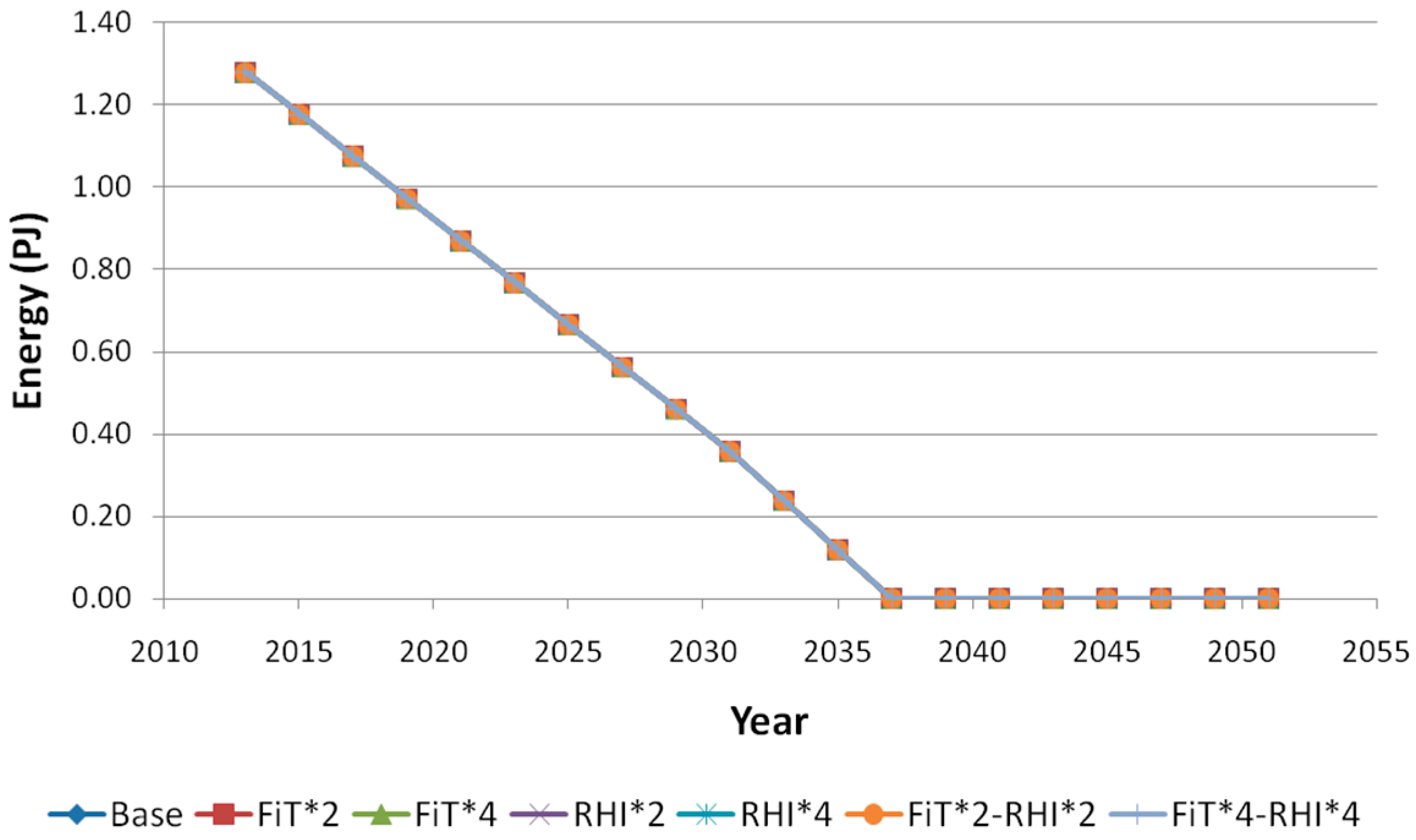
The model results show that in all cases and farm types, the production and use of biogas will increase in the period up to 2021. This is due to a combination of the price of electricity increasing over this period, but also a financial benefit for farmers to employ resources that would otherwise be wasted. The results show that the rates of FiT or RHI do not have any effects on the production rate of biogas, because irrespective of the rate, it is cost-beneficial for farmers to generate as much biogas as possible in order to benefit from the tariffs. Rather, these incentives influence the technology used to convert this biogas into useful energy, whether relatively more expensive CHP or cheaper boilers. In this regard, it was observed that in all cases, farmers invest substantially in biogas production to ensure the maximum use of the feedstocks generated on farms until 2021, after which the tariffs do not apply for new investments. This biogas is then used to either generate heat or electricity and heat, depending on the technology invested by the farms. Hence, we see that grid-fuel usage reduces gradually from 2013 until it is completely reduced in 2037. The fact that the use of all grid-fuel boilers is completely eliminated by 2037 shows that farms will not invest in such boilers from the start of the period, and instead use the residual grid-fuel boilers already in operation until the end of their lifetime of 25 years. This is the most economical way farms can proceed in all cases.

Although the trends for the period of 2013–2021 are generally similar for different rates and farm types, respectively, this period is most consequential for the later energy mix in the simulation. Depending on the electricity/heat use ratio, the energy content of the feedstock, and the tariffs’ rates, farms will determine the type of technology which is most cost-beneficial and what capacity should be installed. These technologies are then used to maximise on the returns from the tariff rates during the period 2021–2045. This is because during this latter period, the tariffs are not valid for new investments, but only for investments in technology installed before 2021, hence the relatively faster pace of most farmers to install the AD technologies prior to 2021. The capacities of the installed technologies are then used during 2021–2045 or until the end of their respective lifetimes, and thus also influence the energy mix close to 2050.

For dairy farms, it was observed that farms will only adopt CHP technologies for “FiT*2”, “FiT*4” and “FiT*4–RHI*4” cases, where the returns generated from adopting CHP technologies are adequate enough to overcome the investment and operating costs, and reduce the overall energy cost of the farms. In the case of “FiT*4”, part of the electricity generated is also exported to the grid. In the other tariff cases, investments are mainly in biogas boilers, with the electricity demand satisfied from grid-electricity supply. However, we also see from Figure 7 that dairy farms will always need to partly depend on the grid for energy supply, as the energy potential from biogas is less than the total energy requirement of such farms.

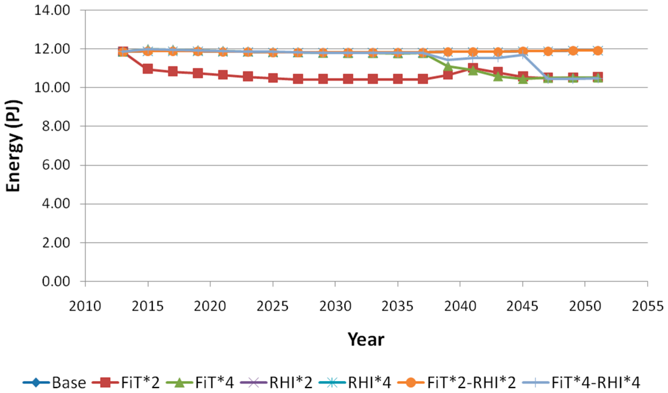
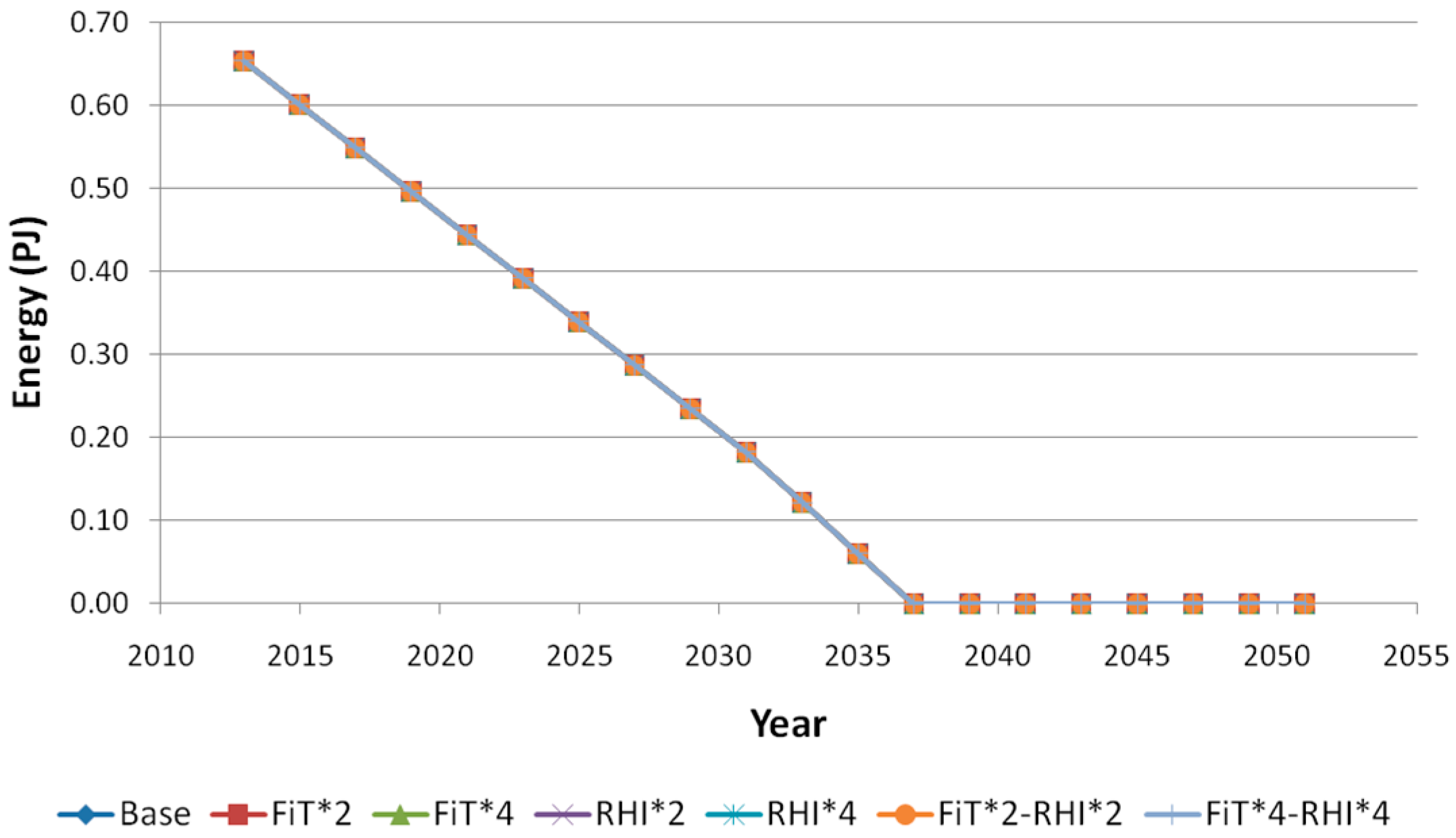
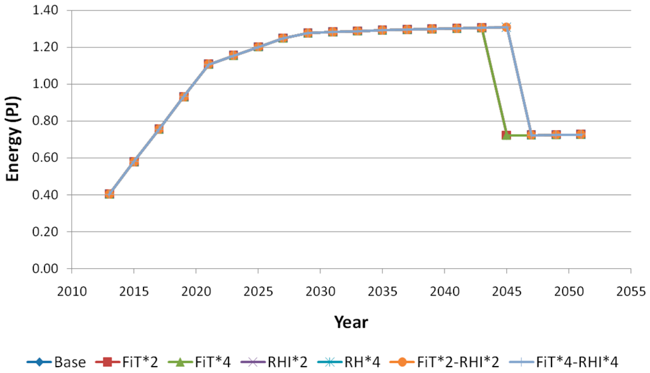
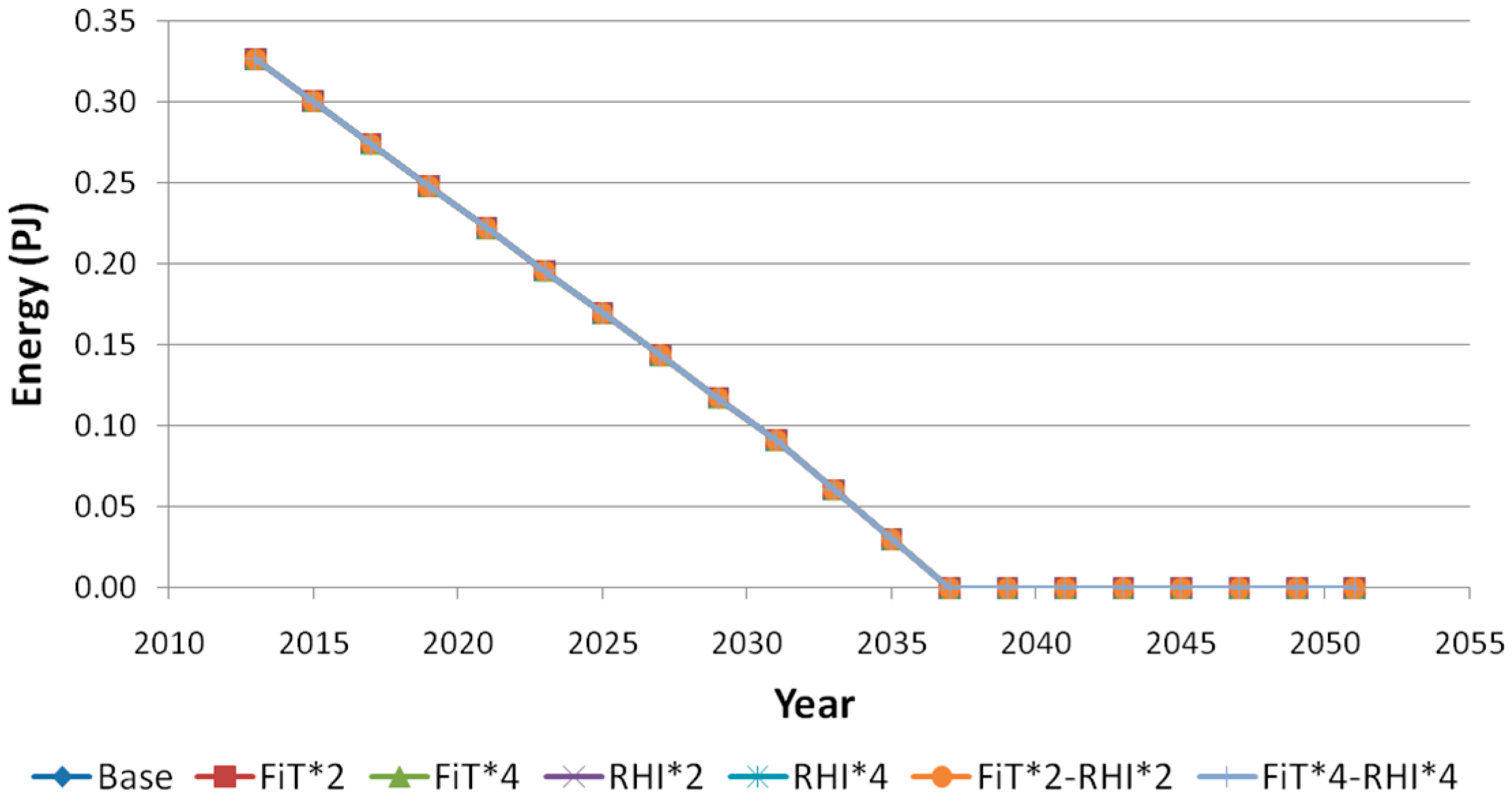
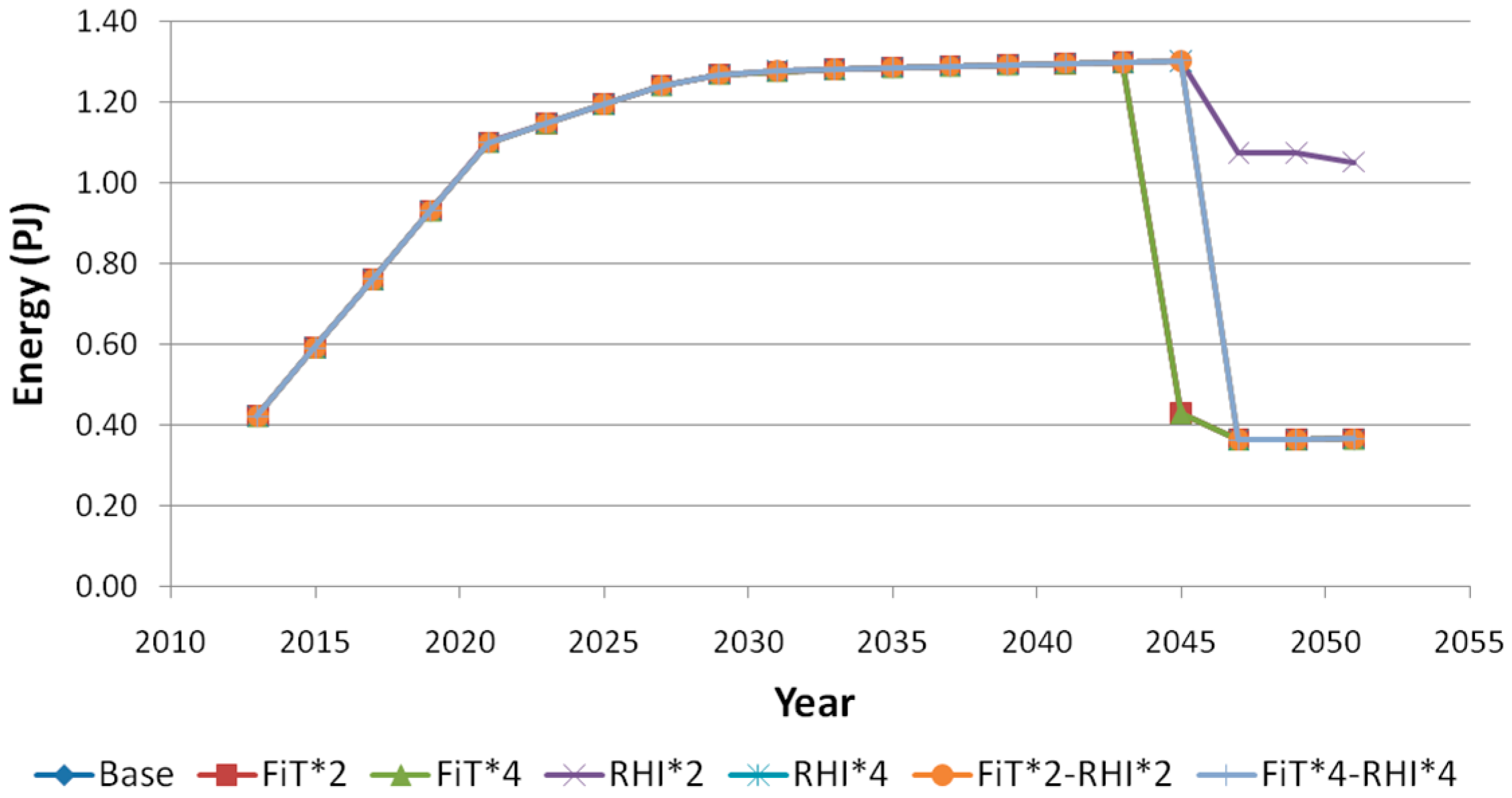
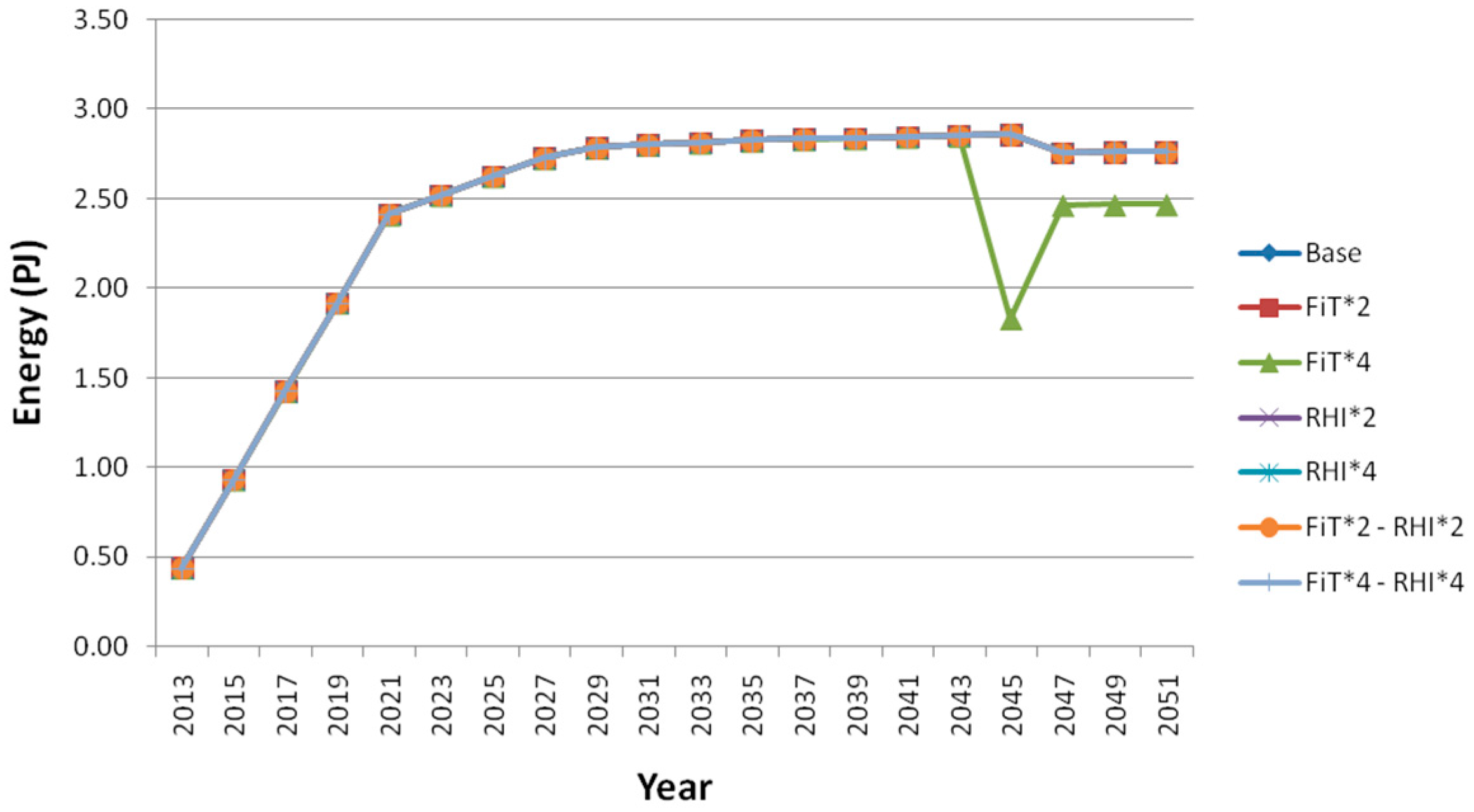
Lowlands farms, although having a pre-existing installed CHP capacity in 2013, is unlikely to sustain any further investments in CHP technology at any FiT or RHI rates. This is partly due to the relatively low electricity-heat ratio of 2.4 compared to other farms, and due to the relatively low energy content of feedstock generated mainly manure from ruminant animals (Table 1). For this farm type, the results show that it is more cost-beneficial to use the biogas generated to produce heat from biogas boilers, and satisfy electricity demand from grid supply over the entire time-horizon. A similar situation is observed for LFA farms whereby it is generally beneficial for LFA farmers to employ the biogas generated to generate heat with biogas boilers, instead of CHP. 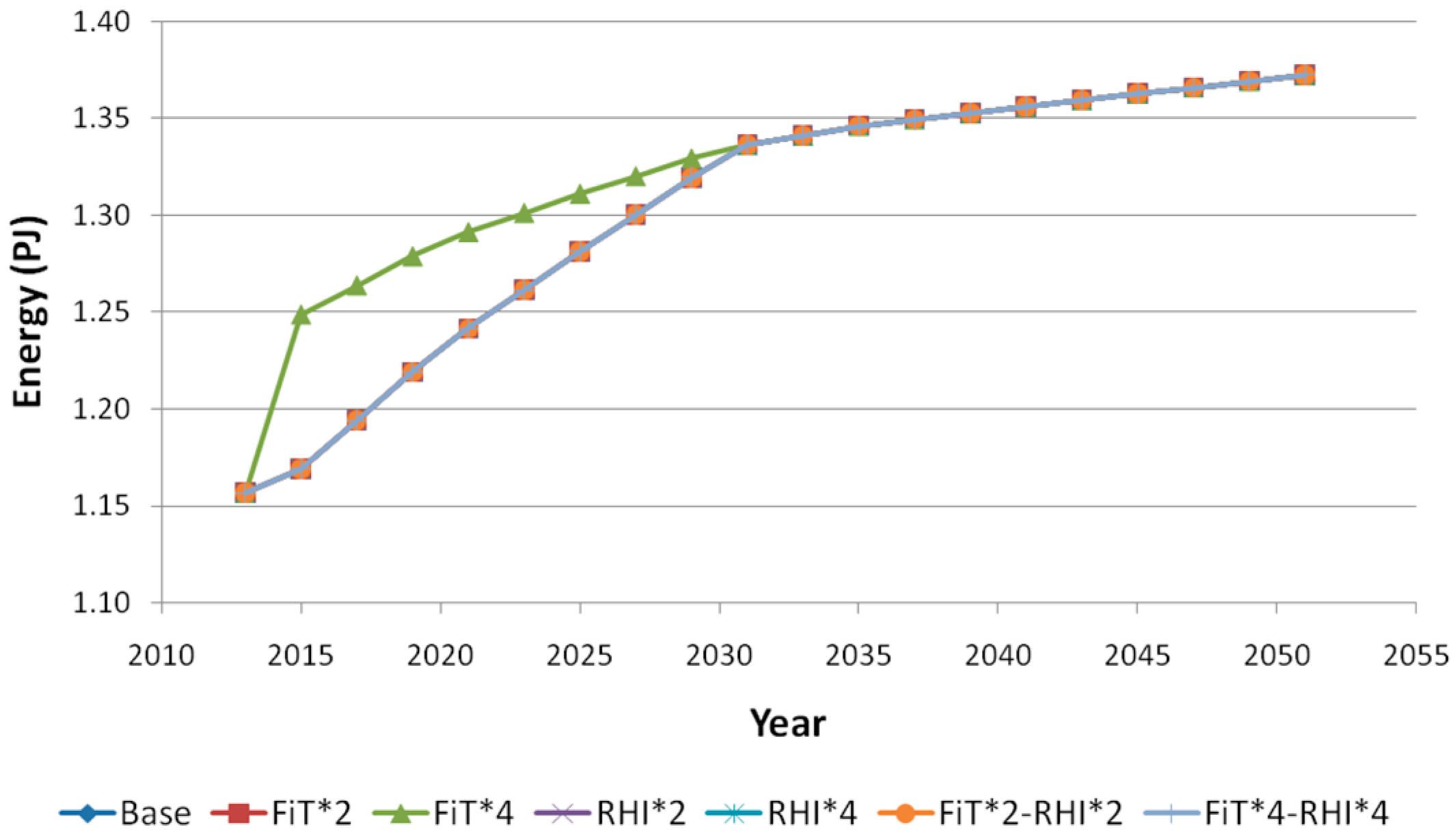The only exception is the case of “RHI*2” (see Figure 13). For this scenario, we observe partial investments in CHP technology which mitigate the demand for grid-electricity in the latter portion of the time-horizon. For LFA farms, because the electricity/heat demand ratio is also relatively low at 2.8, compared to other farms, the RHI rate has a more pronounced effect on the adoption of CHP, as opposed to FiT, as reciprocating CHP technologies produce 1.3 times more heat than electricity which enables farms to have higher return based on the generation of more heat. LFA farms, as opposed to lowlands farms, has the ability to meet its energy requirements from biogas as shown in Figure 12, Figure 13 and Figure 14, where the embedded energy in biogas generated is higher than the total energy demand of LFA farms.

Pig farms were found to have erratic trends with respect to the different FiT and RHI rates studied. These farms have the highest electricity/heat ratio at 127, and for all cases, investing in CHP units will reduce the energy costs of pig farms. The electricity generated will be primarily consumed on-site, although at high “FiT*4” rates, approximately 50%–90% is exported during the period of 2015–2037, to maximise on returns from the tariff. In general, it is beneficial for pig farms to invest in CHP technologies even without any subsidy, however as shown in Figure 16 and Figure 17, under the current high energy demands for electricity and heat, it is impossible for pig farms to become self-sufficient in energy without significant process-efficiency improvement measures.

Poultry farms were found to be more prone to adopting biogas for generating electricity from CHP instead of heat from biogas boilers. Grid electricity demand is seen to reduce to its lowest in 2021, displaced by electricity from CHP, whilst heat demand is satisfied through combinations of biogas boilers and heat generated from CHP. The only exceptions occur at high RHI rates where investments in biogas boilers are more prominent up to 2037, enabling farms to maximise on returns from RHI. Ultimately, however, all FiT and RHI rates favour investments in CHP technology mainly because of the disparity in energy generation potential from biogas (due to high energy content in poultry litter) and the energy demand of farms, and hence the high potential of poultry farms to benefit from the RHI and FiT schemes.

In general, high electricity prices will promote the use of CHP in farms but the degree of adoption will vary depending on the farm type. Farms with high electricity/heat ratio will more easily implement such technologies, whilst other farms may need higher incentives. However, as shown in the cases of pig, poultry, LFA and dairy farms, increasing the FiT rate to high level may lead to the maximisation of generation and export of electricity to the grid, and re-purchasing grid electricity at a relatively cheaper price. The RHI scheme is seen to mainly influence and enhance the competitiveness of biogas boilers, which are already a cheaper investment and operates a higher heat-generating efficiency than CHP technologies. The model generally portrays that the RHI is the main driver behind the adoption of AD in farms and the use of the generated biogas for the production of heat in biogas boilers. In many cases, the heat generation potential is higher than the heat demand of the farm and because of the attractiveness of the incentive; more heat can be generated than is needed. With the unavailability of opportunities to export either heat or biomethane to the grid due to the remote nature of UK farms, the excess heat is wasted and this represents a drawback of the current RHI policy, particularly for farms where the embedded AD feedstock energy may well exceed the energy requirements of the farms, resulting in incentive payments for wasted heat.

5. Conclusions and Policy Implications

The results of this study show that the impact of different rates of the RHI and FiT schemes on different farm types can vary according to the electricity/heat use ratio and the energy content of the feedstock. The analysis showed that for all cases investigated, the adoption of AD can generally be economically attractive to farms. The different rates of the schemes do not consequentially influence the generation of biogas directly, but rather impacts on the competitiveness between the adoption of CHP units and biogas boilers to generate useful energy from the produced biogas. Pig farms which have high electricity/heat ratios will tend to more easily adopt CHP technologies which generate both electricity and heat, whilst other farms will be more inclined towards implementing a mix of technologies, from which biogas boilers will predominate. Although the FiT rates are currently relatively higher per unit energy generated than the RHI, the RHI scheme will generally be more attractive for most farms during the period when the incentives are paying returns. This is due to the cheaper capital and operating costs, as well as the higher heat generation efficiency of boilers compared to CHP, which makes boilers a more cost-competitive technology.

As expected, increasing the FiT rate favours the implementation of CHP units, but excessively high values of four times the current rate may lead to farmers to instead export the generated electricity and re-purchase cheaper electricity from the grid. The higher projected BEIS (former DECC) electricity price will also favour CHP. Increasing the RHI rate simply promotes an already cheap and effective biogas boiler, and is likely to increase heat wastage due to the non-possibility of heat/biomethane export to the grid. Furthermore, even though the schemes are set to end for new applications in 2021, the inertia of their residual effects will be felt until 2041, the end of the tariffs’ lifetime. The type and capacity of technology installed prior to 2021 will likely influence later re-investments by farms between the periods of 2041 and 2050, and therefore impact the energy mix in 2050.

References

1. Energy-Smart Food for People and Climate; Food and Agriculture Organisation (FAO): Roma, Italy, 2011.
2. Renewable Energy Roadmap; URN 11D/698; Department of Energy and Climate Change (DECC): London, UK, 2011.
3. Food Statistics Pocketbook; Department for Environment, Food and Rural Affairs (DEFRA): London, UK, 2013.
4. UK Greenhouse Gas Emissions: Final Figures–Statistical Release; Department of Energy and Climate Change (DECC): London, UK, 2014.
5. Emissions from Livestock; Parliamentary Office of Science and Technology (POST): London, UK, 2014.
6. Anaerobic Digestion; Parliamentary Office of Science and Technology (POST): London, UK, 2011.
7. Jones, P.; Salter, A. Modelling the economics of farm-based anaerobic digestion in a UK whole-farm context. Energy Policy 2013, 62, 215–225. [Google Scholar] [CrossRef]
8. Operational AD Sites; Waste and Resources Action Programme (WRAP): Banbury, UK, 2015.
9. German Biogas; German Biogas Association: Freising, Germany, 2015.
10. Tranter, R.B.; Swinbank, A.; Jones, P.J.; Banks, C.J.; Salter, A.M. Assessing the potential for the uptake of on-farm anaerobic digestion for energy production in England. Energy Policy 2011, 39, 2424–2430. [Google Scholar] [CrossRef]
11. Energypedia. Available online: https://energypedia.info/wiki/Costs_of_a_Biogas_Plant#Capital_Costs (accessed on 1 May 2015).
12. Bywater, A.M. A Review of Anaerobic Digestion Plants on UK Farms-Barriers, Benefitsand Case Studies; Royal Agricultural Society of England: Warwickshire, UK, 2011. [Google Scholar]
13. Feed-in Tariff Payment Rate Table for Non-Photovoltaic Eligible Installations for FIT Year 4; Ofgem: London, UK, 2015.
14. Tariff That Apply for Non-Domestic RHI for Great Britain; Ofgem: London, UK, 2015.
15. Anaerobic Digestate: End of Waste Criteria for the Production and Use of Quality Outputs from Anaerobic Digestion of Source-Segregated Biodegradable Waste; Waste and Resources Action Programme (WRAP): Banbury, UK; Environment Agency: Bristol, UK, 2014.
16. A Survey of the UK Anaerobic Digestion Industry in 2013; Waste and Resources Action Programme (WRAP): Banbury, UK, 2013.
17. Mistry, P.; Smith, I. Bringing small scale AD to UK farmers—The challenge. In Proceedings of the European Bioenergy Expo and Conference, Warwickshire, UK, 6–7 October 2010.
18. Dolan, T.; Cook, M.B.; Angus, A.J. Financial appraisal of wet mesophilic AD technology as a renewable energy and waste management technology. Sci. Total Environ. 2011, 409, 2460–2466. [Google Scholar] [CrossRef] [PubMed]
19. Zglobisz, N.; Castillo-Castillo, A.; Grimes, S.; Jones, P. Influence of UK energy policy on the deployment of anaerobic digestion. Energy Policy 2010, 38, 5988–5999. [Google Scholar] [CrossRef]
20. AD Cost Calculator: Economic Assessment of Anaerobic Digestion Technology & its Suitability to UK Farming & Waste Systems (Tool), NNFCC 10-010; National Non-Food Crops Centre (NNFCC): York, UK; The Andersons Centre: Leicestershire, UK, 2013.
21. Kassier, W.E. An application of linear programming to farm planning. S. Afr. J. Econ. 1963, 31, 118–126. [Google Scholar] [CrossRef]
22. Ballarin, A.; Vecchiato, D.; Tempesta, T.; Marangon, F.; Troiano, S. Biomass energy production in agriculture: A weighted goal programming analysis. Energy Policy 2011, 39, 1123–1131. [Google Scholar] [CrossRef]
23. Jablonski, S.; Strachan, N.; Brand, C.; Bauen, A. The role of bioenergy in the UK’s energy future formulation and modelling of long-term UK bioenergy scenarios. Energy Policy 2010, 38, 5799–5816. [Google Scholar] [CrossRef]
24. Seck, G.S.; Guerassimoff, G.; Maizi, N. Heat recovery with heat pumps in non-energy intensive industry: A detailed bottom-up model analysis in the French food & drink industry. Appl. Energy 2013, 111, 489–504. [Google Scholar]
25. Loulou, R.; Goldstein, G.; Noble, K. Documentation for the MARKAL Family of Modelss; Energy Technology System Analysis Programme (ETSAP): Paris, France, 2004. [Google Scholar]
26. Anaerobic Digestion. Feedstocks. Available online: http://www.biogas-info.co.uk/about/feedstocks/#crops (accessed on 5 October 2015).
27. Farm Accounts in England 2013/2014; Department for Environment, Food and Rural Affairs (DEFRA): London, UK, 2014.
28. Hopwood, L. Farm-Scale Anaerobic Digestion Plant Efficiency; National Non-Food Crops Centre (NNFCC): York, UK, 2011. [Google Scholar]
29. Fogerty, M.; Soffe, R.; Robbins, K. Farm Business Survey—2011/2012—Lowland Grazing Livestock Production in England; Royal Agricultural Society of England (RASE): Kenilworth, UK, 2012. [Google Scholar]
30. European Commission. Available online: http://ec.europa.eu/agriculture/rurdev/lfa/index_en.htm (accessed on 23 July 2015).
31. Average Number of Poultry Slaughtered Per Week in the UK; Department for Environment, Food and Rural Affairs (DEFRA): London, UK, 2015.
32. Gowreesunker, B.L.; Tassou, S.A. Energy generation potential of anaerobic digestion from the food and farming wastes of the UK food chain. Renew. Bioresour. 2014, 2, 4. [Google Scholar] [CrossRef]
33. Clarke-Energy. Available online: http://www.clarke-energy.com/2013/chp-cogen-efficiency-biogas/ (accessed on 3 August 2015).
34. Steam and High Temperature Hot Water Boilers—CTV 052; The Carbon Trust: London, UK, 2012.
35. ICAX. Available online: http://www.icax.co.uk/RHI_Tariff_Degression.html (accessed on 20 August 2015).
36. Marches Biogas. Available online: http://www.marchesbiogas.com/ad_explained (accessed on 20 August 2015).
37. Yougen. Available online: http://www.yougen.co.uk/feed-in-tariff/ (accessed on 20 August 2015).
38. Updated Energy and Emissions Projections: 2015—Annex M: Growth Assumptions and Prices; Department of Energy and Climate Change (DECC): London, UK, 2014.
39. Baffes, J.; Cosic, D.; Kshirsagarm, V. Commodity Market Outlook; World Bank Group: Washington, DC, USA, 2014. [Google Scholar]
40. Patton, M.; Feng, S.; Davis, J.; Binfield, J. Impact of CAP Post-2013 Reforms on Agriculture in the UK: FAPRI Project Report; Department for Environment, Food & Rural Affairs (DEFRA): London, UK, 2013.
Figure 1. Sectors employing anaerobic digesters (AD) units in Great Britain (GB) [8].
Energies 09 01038 g001
Figure 2. (a) Feed-in tariff (FiT) and (b) renewable heat incentive (RHI) rates trend for AD.
Energies 09 01038 g002
Figure 3. Technical information flow and applied incentives in GB farms. CHP: combined heat and power.
Energies 09 01038 g003
Figure 4. (a) Projected electricity prices; (b) projected fuel prices (kerosene/gas-oil); and (c) projected fertiliser prices (average of nitrogen, potash and phosphate based fertilisers).
Energies 09 01038 g004
Figure 5. Total animal projections in farms.
Energies 09 01038 g005
Figure 6. Dairy farms—fuel consumption.
Energies 09 01038 g006
Figure 7. Dairy farms—grid electricity consumption.
Energies 09 01038 g007
Figure 8. Dairy farms—biogas production.
Energies 09 01038 g008
Figure 9. Lowlands farms—fuel consumption.
Energies 09 01038 g009
Figure 10. Lowlands farms—grid electricity consumption.
Energies 09 01038 g010
Figure 11. Lowlands farms—biogas production.
Energies 09 01038 g011
Figure 12. Less-favourable area farms (LFA) farms—fuel consumption.
Energies 09 01038 g012
Figure 13. LFA farms—grid electricity consumption.
Energies 09 01038 g013
Figure 14. LFA farms—biogas production.
Energies 09 01038 g014
Figure 15. Specialist pig farms—fuel consumption.
Energies 09 01038 g015
Figure 16. Specialist pig farms—grid electricity consumption.
Energies 09 01038 g016
Figure 17. Specialist pig farms—biogas production.
Energies 09 01038 g017
Figure 18. Specialist poultry farms—fuel consumption.
Energies 09 01038 g018
Figure 19. Specialist poultry farms—grid electricity consumption.
Energies 09 01038 g019
Figure 20. Specialist poultry farms—biogas production.
Energies 09 01038 g020