
Physical Background, Computations and Practical Issues of the Magnetohydrodynamic Pressure Drop in a Fusion Liquid Metal Blanket


Department of Mechanical and Aerospace Engineering, University of California, Los Angeles, CA 90095, USA
Fluids 2021, 6(3), 110; https://doi.org/10.3390/fluids6030110
Submission received: 6 February 2021
/
Revised: 2 March 2021
/
Accepted: 4 March 2021
/
Published: 8 March 2021
(This article belongs to the Special Issue Fluids in Magnetic/Electric Fields)
Abstract
:In blankets of a fusion power reactor, liquid metal (LM) breeders, such as pure lithium or lead-lithium alloy, circulate in complex shape blanket conduits for power conversion and tritium breeding in the presence of a strong plasma-confining magnetic field. The interaction of the magnetic field with induced electric currents in the breeder results in various magnetohydrodynamic (MHD) effects on the flow. Of them, high MHD pressure losses in the LM breeder flows is one of the most important feasibility issues. To design new feasible LM breeding blankets or to improve the existing blanket concepts and designs, one needs to identify and characterize sources of high MHD pressure drop, to understand the underlying physics of MHD flows and to eventually define ways of mitigating high MHD pressure drop in the entire blanket and its sub-components. This article is a comprehensive review of earlier and recent studies of MHD pressure drop in LM blankets with a special focus on: (1) physics of LM MHD flows in typical blanket configurations, (2) development and testing of computational tools for LM MHD flows, (3) practical aspects associated with pumping of a conducting liquid breeder through a strong magnetic field, and (4) approaches to mitigation of the MHD pressure drop in a LM blanket.
1. Introduction
Development of a reliable, low-cost, and safe blanket system of a fusion power reactor that provides self-sufficient tritium breeding and efficient conversion of the extracted fusion energy to electricity, while meeting all material, design, and configuration limitations is among the most important fusion science and technology goals [1]. In the liquid metal (LM) blanket concepts, lithium-containing LMs are used to breed tritium with pure lithium (Li) and the eutectic lead-lithium alloy (PbLi) as the primary candidates. Such LMs can provide sufficient tritium breeding ratio and have high thermal conductivity (~101 W/m-K) and low viscosity (~10−7 m2/s) that make them very favorable for heat removal. PbLi is considered by many researchers as a more attractive breeder/coolant option than pure Li due to its lower chemical reactivity with water, air and concrete, but PbLi is more corrosive and has higher density and more undesirable activation products.
Among several feasibility constraints of LM blankets, magnetohydrodynamic (MHD) pressure drop is often considered as the most serious issue [2]. In a blanket, pure Li or PbLi circulates in complex-geometry circuits in presence of a strong plasma-confining magnetic field (4–10 T) to produce tritium and to remove heat generated by fusion neutrons. The flow of the electrically conducting breeder (σ ~ 106 S/m) in a strong magnetic field induces electric currents, which, in turn, interact with the magnetic field resulting in strong flow opposing electromagnetic Lorentz forces, which can be several orders of magnitude higher than viscous and inertial forces in ordinary flows. The associated MHD pressure drop is typically high (up to several MPa), and can be unacceptable, because of several reasons:
- -
- Mechanical stresses in the structural walls are above the materials limit;
- -
- High pumping power that diminishes the overall blanket efficiency;
- -
- Unavailability of high capacity LM pumps.
In accordance with the “Blanket Comparison and Selection Study” (BCSS) in the US [3], the maximum MHD pressure drop in a blanket should be limited to 2 MPa. Most of the blanket designs for which the pressure drop was demonstrated to be lower than 2 MPa meet the stress and pumping power requirements. Higher pressure drops might still be allowed but this needs to be confirmed through the thermo-mechanical analysis. Such an analysis might also require data on the pressure drop in the ancillary equipment as the entire pressure drop in the LM circuit is composed of the MHD pressure drop in the blanket and the ordinary pressure drops in the ancillary components, such as a tritium extraction system and a heat exchanger, where LM flows do not experience MHD effects but are typically turbulent.
To design new feasible LM breeding blankets or to improve the existing blanket concepts and designs, one needs to identify and characterize sources of high MHD pressure drop, to understand the underlying physics of MHD flows and to eventually define ways of mitigating high MHD pressure drops in the entire blanket and its sub-components. The corresponding analysis requires significant involvement of Magnetohydrodynamics, the discipline that studies flows of electrically conducting fluids in a magnetic field. Several monographs on liquid metal Magnetohydrodynamics [4,5,6,7,8,9,10,11,12] pay special attention to LM MHD flows in fusion applications. In particular, Ref. [12] has a dedicated chapter on “Liquid Metal Magnetohydrodynamics for Fusion Blankets” by L. Bühler. Many journal reviews of MHD flows under blanket relevant conditions were also published over last several decades [2,13,14,15,16,17,18], with significant emphasis on the pressure drop and related aspects of MHD flows. Dedicated MHD studies aimed at the evaluation of the MHD pressure drop for particular LM blanket concepts and designs were performed at different times in [19] for a self-cooled PbLi blanket, [20,21] and [22] for a DCLL blanket, [23,24] for HCLL blanket, and [25] and [26] for a WCLL blanket.
This article summarizes earlier and recent studies of MHD pressure drop in LM blankets with a special focus on (1) physics of LM MHD flows in typical blanket configurations, (2) development and testing of computational tools for LM MHD flows, (3) practical aspects associated with pumping of a conducting liquid breeder through a strong magnetic field, and (4) approaches to mitigation of the MHD pressure drop in a LM blanket.
2. Examples of LM Breeding Blankets and Their Pressure Drop
During recent decades, various LM blanket concepts were proposed and intensively studied worldwide, including self-cooled, separately cooled and dual-coolant blankets. Historically, self-cooled blanket concepts were the first to be considered. Self-cooled concepts have potential for simplifying the blanket design significantly, but studies found that the high velocity needed to cool the first wall resulted in untenable MHD effects such as large pressure drop. The high magnetohydrodynamic (MHD) pressure drop required at high flow rates resulted in pressure stresses exceeding the allowable structural material limits. Electric insulators for the first wall region (e.g., coatings) as a means of reduction of the MHD pressure drop have not been successfully developed. To solve the MHD problem, the separately cooled blankets were proposed, where the LM serves only as a breeder material while all the surface and volumetric heat is removed by a coolant like water or helium (He) gas. The separately cooled blanket concept suffers from low coolant exit temperature dictated by the maximum allowable temperature of the structural material. Additionally, the concept still suffers from some MHD effects due to magnetic field transients and the need to circulate the liquid metal for tritium recovery. A combination of both ideas led to proposing the dual-coolant blanket concept, where the surface heat flux on the first wall is removed by a He coolant, while the liquid metal is used for “self-cooling” in the breeder zone. Typical examples that illustrate these LM blanket concepts are presented below.
The US Self-cooled Lithium blanket with the vanadium alloy as the structural material [3] is a typical example of self-cooled blankets. Although this concept was ranked highest in BCSS, its further development was suspended about 30 years ago due to low tolerance of insulating coatings to cracks and other insulation defects that are likely to occur and give raise to unacceptably high MHD pressure drop. Mainly because of this reason, almost no considerations are given to this concept nowadays. In this design, a toroidal–poloidal configuration is maintained to minimize the MHD pressure drop and to provide high heat flux removal capabilities at the same time.
The design (Figure 1) is composed of slightly slanted poloidal manifolds and relatively small toroidal channels where the Li velocity can be as high as 0.5–1 m/s to provide high heat removal capability. The toroidal channels are exposed to both the surface heat flux and volumetric nuclear heating. The poloidal manifold is protected by the toroidal channels both thermally from the surface heat flux and structurally from radiation damage. A large cross-sectional area is maintained for the poloidal manifold to keep the velocity low to reduce the MHD pressure drop. Although the toroidal flows do not create significant MHD pressure drops, large pressure losses occur when the liquid changes its direction from toroidal to poloidal. As a result, the overall pressure drop may exceed the nominal pressure drop limit of 2 MPa. As a means of reducing the MHD pressure drop, thin insulating coatings were proposed but, as mentioned above, their ability to tolerate small defects in the insulation is still questionable.
The Helium-Cooled Lead Lithium (HCLL) blanket [27] belongs to the class of separately cooled blankets. In the EU, this blanket concept is considered as a possible option for implementation in DEMO reactor and future power plants. It was also planned as a test blanket module (TBM) for testing in ITER until the recent change to the Water-Cooled Lead Lithium (WCLL) blanket [28]. The HCLL concept (Figure 2) relies on available structural materials and fabrication techniques but has much lower thermal efficiency and higher tritium loss compared to the DCLL blanket. In the HCLL, PbLi serves exclusively as a breeder material circulating at a very low velocity of 0.1–1 mm/s while the entire thermal power released in the blanket is removed by a He-cooling system. The MHD pressure drop in the blanket itself is relatively low but that in the feeding ducts is expected to be high due to higher velocities compared to the blanket channels. Reference [29] reports maximum pressure drop of 0.332 MPa in outboard segment and 0.230 MPa in inboard segment of the EU DEMO HCLL blanket. Tritium permeation from PbLi into He flows is a serious safety issue for all HCLL blankets. Thus, it has to be ensured that all breading units in the HCLL have no stagnant flow regions to avoid high tritium losses.
The Dual-Coolant Lead Lithium (DCLL) blanket [30] concept promises a solution toward a high-temperature, high-efficiency blanket while using temperature-limited RAFM (Reduced Activation Ferritic/Martensitic) steel as structural material.
In this concept (Figure 3), a high-temperature PbLi alloy flows slowly (velocity ~ 10 cm/s) in large poloidal rectangular ducts (duct size ~ 20 cm) to remove the volumetric heat and produce tritium, while the pressurized He gas (typically to 8 MPa) is used to remove the surface heat flux and to cool the ferritic first wall and other blanket structures to <550 °C. A few millimeter thick, low-conductivity flow channel insert (FCI) made of SiC ceramics is used for electrical and thermal insulation. The FCI is the most critical element of the DCLL blanket concept that needs to be qualified before the FCI could be implemented in a future blanket. Several papers report the overall MHD pressure drop ΔP in a DCLL blanket around or smaller than 2 MPa. For example, the MHD pressure drop in the DCLL blanket of the US DEMO reactor was estimated at 0.4 MPa for the outboard (OB) and 1.17 MPa for the inboard (IB) blanket module [20]. Estimates in [21] for the US Fusion Nuclear Science Facility (FNSF) suggest ΔP = 0.98 MPa for the IB blanket and ΔP = 2.25 for the OB blanket. It is interesting that the total pressure drop in the OB blanket in [21] is more than two times higher compared to the IB blanket even though the magnetic field at the inboard is almost two times higher compared to the outboard. This result is different from conclusions in [20] and similar studies, where the IB pressure drop was always found to be higher than that at the OB. This surprising conclusion can be explained by combination of several factors, such as larger dimensions of the OB blanket, longer poloidal flow path, and higher neutron wall loading resulting in higher velocities in all OB blanket components.
There are two approaches to the DCLL blanket configuration as shown in Figure 4. A full segment “banana” DCLL blanket (poloidal length ~10 m) stretches all the way from the bottom to the top of the vacuum chamber as that in the US FNSF design [21]. Contrary to this, the EU DCLL DEMO design [22] has a modular structure where several modules of about 2 m each are fed from the shared manifold situated at the back of the blanket. To our best knowledge, there has been no comparison analysis of the MHD pressure drop between the “banana” and modular blanket for the same fusion reactor and operation parameters. Therefore, it is not obvious which blanket configuration is advantageous in terms of the MHD pressure drop. Although the “banana” blanket has a long poloidal flow path, in the modular blanket the flow circuit is more complex, so that higher pressure losses can be expected in the modular blanket.
The Water-Cooled Lead Lithium (WCLL) blanket [31] also belongs to the class of separately cooled blankets, similar to the HCLL concept. However, unlike the HCLL, cooling is performed with water at pressurized water reactor (PWR) conditions (water pressure 15.5 MPa, Tin/Tout = 285 °C/325 °C). Since PWR is a mature technology, many fusion researchers consider that only small extrapolation from present-day knowledge both on physical and technological aspect is needed for a feasible WCLL blanket [31]. In the EU, this blanket concept is considered for testing in ITER, and also as a likely candidate for implementation in the EU DEMO reactor. In the US, water has not been chosen as a fusion power core coolant for decades because of potential safety issues associated with hydrogen generation in case of water-lithium reactions. In the WCLL concept (Figure 5), PbLi alloy serves as breeder, neutron multiplier and tritium carrier, while “Eurofer” RAFM steel is used as structural material. The breeder slowly recirculates in the blanket making 10–50 recirculations a day (flow velocity ~ 1 mm/s). All heat generated in the blanket is removed with water flowing in numerous double-walled tubes. Since tritium can permeate through the steel wall of the water pipes into cooling water, tritium extraction is required from both PbLi and water.
The PbLi MHD pressure drop in a simplified version of the WCLL blanket was estimated in [32] using numerical computations. Due to the low PbLi velocity, the overall pressure drop of the elementary WCLL cell was found to be only 2055 Pa. This is significantly lower compared to other LM blanket concepts. Recent detailed analysis of a full WCLL blanket design in [33] suggests significantly higher MHD pressure drops, 1.609 MPa for the outboard and 2.435 MPa for the inboard module, such that insulating flow inserts or other insulating techniques may be required to reduce the MHD pressure drop, especially for the feeding/collecting pipes at the entrance/exit of the inboard module.
3. Mathematical Formulation of the Problem
3.1. Governing Equations of LM MHD Flows
A sketch in Figure 6 shows a prototypic pressure-driven LM flow configuration, featuring a complex geometry thin-walled duct, applied magnetic field , ), volumetric heating , and gravity g = (g, 0, 0). The flow can change its direction and the duct can experience variations of the cross-sectional area along its axis as shown in the figure. Such a flow induces its own magnetic field , so that the total magnetic field is a superposition of the applied and induced one: . The associated induced electric current j) interacts with the magnetic field resulting in the electromagnetic Lorentz force opposing the flow. The flow in a blanket can also be affected by buoyancy forces that arise in the liquid due to density variations caused by neutron volumetric heating. A mathematical model for such a flow can be formulated in several ways, including a few choices for main variables, various approximations and coordinate systems (see, e.g., discussion in [34]).
All mathematical models of 3D LM MHD flows include the modified Navier–Stokes equations, energy equation and electromagnetic equations, which can be deduced from Maxwell’s equations. The fluid flow equations coupled with the energy equation are written below in Cartesian coordinates x, y and z, using velocity V = (, V, W), pressure P, and temperature T as the main variables. Two basic approximations are employed. One is the so-called inductionless approximation (also known as the low magnetic Reynolds number approximation), where induced magnetic field is neglected compared to the applied one such that the Lorentz force term can be written using only applied magnetic field: . The second one is the Boussinesq approximation, in which fluid density differences are ignored except where they appear in the buoyancy force term.
The three projections of the momentum equation on the coordinate axes include the electromagnetic Lorentz force. Equation (1) for the vertical velocity component also includes a temperature dependent term associated with the buoyancy forces. The velocity field is solenoidal so that the mass conservation equation Equation (4) applies. The temperature field is described by the energy equation Equation (5) with the volumetric source term on its right-hand-side. In the energy equation, the Joule and viscous dissipation are neglected because in a LM blanket they are much smaller than the volumetric heating. The physical properties in the mathematical model are defined at the reference temperature T0: ρ is the density, ν is the kinematic viscosity, is the thermal expansion coefficient, is the specific heat, σ is the electrical conductivity and k is the thermal conductivity. Equations (1)–(5) can be used for both laminar and turbulent flows. It should be noted that the equations neglect some molecular non-equilibrium effects on the temperature and velocity filed, such as magnetization, polarization or Peltier, Thompson, Seebeck and Doufour effects, which under the blanket conditions are weak compared to others [10].
The system of Equations (1)–(5) is not closed unless electromagnetic equations are added, from which the induced electric current can be computed. An electromagnetic formulation based on the scalar electric potential as the principal electromagnetic variable is perhaps the most common one. With the help of , the induced electric current can be computed using Ohm’s law:
In turn, the electric current has to satisfy the charge conservation equation:
Equations (6) and (7) can be combined together resulting in an elliptic Poisson equation from which the electric potential and then the current density components can be computed:
Altogether, Equations (1)–(8) make a closed set of equations that need to be solved simultaneously in a multi-material domain composed of the electrically conducting liquid and a solid wall that, in general, has different physical properties than the liquid. In doing so, Equations (1)–(4) are applied to the liquid only, while Equations (5)–(8) to the entire domain. It needs to be stressed that the electric potential based formulation is valid as long as the induced magnetic field is much smaller than the applied one [8]. This in turn implies that the dimensionless magnetic Reynolds number Rem = L/νm has to remain much smaller than unity. This is typically the case in almost all liquid metal flows in a blanket due to the relatively low breeder velocities , small characteristic blanket dimension L, and high magnetic viscosity νm. One possible exception is the plasma disruption scenario [35], where the transients in the magnetic field may result in very high LM velocities of the order of ~102 m/s [36], such that Rem > 1. In such abnormal scenarios, the induced magnetic field cannot be neglected anymore, therefore the full magnetic induction formulation has to be used. The obvious advantage of the -formulation, especially in the case of numerical computations, is that only one elliptic electromagnetic equation Equation (8) is required. The utilization of the magnetic field-based formulation requires three elliptic equations to be solved in a larger computational domain that includes not only the blanket but also some surrounding space (“vacuum”), where the induced magnetic field vanishes. This implies a significant computational effort compared to the -formulation as solving elliptic equations is the most time-consuming part of the computations. When using the B-formulation, the electric current can be computed with the help of Ampèr’s law:
Several numerical examples where the B-formulation was employed are given in [37], including cases at Rem << 1, Rem ~ 1 and Rem >> 1.
In addition to the - and B-formulation, we can refer to several electromagnetic formulations of considerable use that implement the magnetic vector potential A, as well as the current vector potential T or some combinations of the above quantities, for instance A − [38]. Attempts on implementation of a formulation making use of the induced electric current j as the main electromagnetic variable are relatively recent. The equations for the induced electric current and thin wall boundary conditions were derived in [34]. The suggested formulation (denominated “j-formulation”) was then applied in the finite-difference computations of three common types of MHD wall-bounded flows: (i) high Hartmann number fully developed flows in a rectangular duct with conducting walls; (ii) quasi-two-dimensional duct flow in the entry into a magnet; and (iii) flow past a magnetic obstacle.
Once the velocity field, temperature field and electric current density are known, the pressure field can be evaluated by solving a Poissson equation for pressure, which is derived by taking a derivative of each projection of the momentum equation with respect to the corresponding coordinate and then adding all equations together:
where
The first source term on the right-hand side of Equation (10) is associated with the fluid motion. The second term is of electromagnetic nature. The third term reflects the effect of the axial temperature gradient in the fluid.
3.2. Boundary Conditions
To accomplish the mathematical formulation, boundary conditions need to be added. They are comprised of those at the solid–liquid interfaces, inlet/outlet boundary conditions and those at the outer surface of the flow-confining electrically conducting solid walls. At the liquid-solid interface, it is assumed that the viscous liquid sticks to the rigid wall so that the so-called “no-slip” condition is applied, V = 0. In rare cases, for example at the interface between the PbLi breeder and SiC ceramics, a “slip” boundary condition may serve as a more appropriate condition: V = Vs, where Vs is the “slip” velocity [39]. If there is no contact resistance between the liquid and the wall, the electrical contact is perfect. This implies the wall-normal component of the electric current and the electric potential to be continuous across the interface: and . The tangential component of the current experiences a discontinuity at the interface: because the electrical conductivity of the wall is in general different from that of liquid . When the electrically conducting wall is “thin”, i.e., the wall thickness tw is much smaller than the characteristic duct dimension L, tw << L, the so-called thin-wall boundary condition can be used [40]. Physically, the thin-wall boundary condition means that the electric current enters the thin wall from the liquid and then flows there in the tangential direction so that the electric potential does not vary across the wall to the leading order of approximation. This condition allows reducing the solution of Equation (6) to the fluid region. In the case of a “thick” conducting wall, the boundary conditions on the electric potential have to be imposed at the outer surface of the wall to enforce the wall-normal current density component to be zero. The temperature boundary conditions can be one of the three types, Dirichlet, Neumann or Robin, and can be imposed either at the liquid-solid interface or at the outer wall depending on the problem.
Entrance and exit conditions depend on the specific flow configuration and operating conditions. For substantially long ducts in a constant transverse magnetic field, a fully developed velocity and current distribution, constant temperature and zero gradient pressure can be imposed as the inlet boundary condition. At the outlet, an outflow boundary condition is often used for all quantities except for the pressure. The simplest and most commonly used outflow condition is that of a “continuative” boundary. Continuative boundary conditions consist of zero normal derivatives. This zero-derivative condition is intended to represent a smooth continuation of the flow through the outlet boundary. The pressure outlet boundary condition requires a constant pressure that can be set to zero.
3.3. Dimensionless Form of of Governing Equations and Basic Dimensionless Numbers
The governing equations of the LM MHD flow and the boundary conditions can be written in a dimensionless form, which is more tractable for order of magnitude analysis. In doing so, appropriate characteristic quantities (scales) are used: as the velocity scale, as a scale for the magnetic field, L as a characteristic dimension, and the characteristic temperature difference in the fluid is used as a temperature scale. From these basic scales, other scales can be constructed: L/ is the time scale, is the pressure scale, is the scale for the electric potential, and is the scale for the electric current density. When dividing each dimensional quantity by its scale, the governing equations take the following form:
Here, the equations are written in the compact vector form. Symbol “tilde” indicates that the corresponding quantity is made dimensionless. The dimensionless electrical and thermal conductivities and are equal to 1 within the liquid. Within the wall, and . The equations include fundamental dimensionless groups Re, Ha, N, Fr and Gr numbers that express ratios between various forces in the flow. The hydrodynamic Reynolds number is the ratio of the inertia to viscous forces. The Hartmann number squared () expresses the ratio between the electromagnetic and viscous forces. The Stuart number (also known as the interaction parameter) N = Ha2/Re is the ratio of electromagnetic to inertia forces. The Froude number is the ratio of inertia to gravity. The Grashof number is the ratio between the buoyancy and viscous forces. The characteristic temperature difference in Gr is typically defined using the so-called neutron wall load (NWL), which is the integral of over the radial depth of the blanket. For different LM blanket concept and designs, the NWL changes in the range from 0.7 MW/m2 to 2.5 MW/m2. One more dimensionless parameter, Pr = νCp/, is the Prandtl number, which is the ratio of momentum diffusivity to thermal diffusivity. Its small value in liquid metals of ~0.01 indicates that the heat diffusion in the liquid breeder dominates over the convection transport. For MHD flows in thin-walled ducts, another dimensionless parameter called “wall conductance ratio” can also be constructed that characterizes the electrical conductance of the wall in comparison with the conductance of the liquid: This parameter, which in blanket applications is typically much smaller than unity, strongly influences the MHD pressure drop in all LM blanket concepts unless the walls are electrically insulated. Typical values of the key dimensionless parameters for the blanket concepts introduced in Section 2 of this paper are shown in Table 1.
In what follows, we will consider a few particular flow geometries, including straight rectangular ducts with the cross section and circular pipes with the radius R. Unless otherwise specified, the half-width of the duct b in the direction of the applied magnetic field (“Hartmann length”) and dimension R in the case of pipe flows are used as a characteristic length in the definition of all dimensionless parameters. The mean velocity defined as (integration is performed over the cross-sectional area S) is used as the velocity scale.
4. Special Classes of MHD Flows in a LM Blanket
4.1. Fully Developed MHD Flows
If the LM carrying duct of a blanket is long enough (typically more than a few characteristic cross-sectional lengths) and the applied magnetic field does not exhibit significant variations along the flow path, as it happens for example in poloidal flows of the DCLL blanket, the flow is likely to become fully developed. In the fully developed flows, inertia forces are zero. The main forces acting on the flow are those due to viscous friction, pressure, electromagnetic interaction, and buoyancy effects. Bellow, equations for a fully developed flow in a uniform transverse magnetic field are derived from the full equations without considering buoyancy forces. The basic characteristic features of fully developed flows allow for significant simplifications of the governing equations making the MHD problem more tractable for analytical studies, including analysis of the MHD pressure drop. By definition, in the fully developed flow, the axial velocity component does not depend on the axial coordinate x: = (y,z). The other two velocity components V and W in the plane of the applied magnetic field are zero. The pressure does not vary within the duct cross-sectional area but changes linearly with the axial coordinate, such that the pressure gradient in the fluid is constant: −dP/dx = Const(x,y,z). Other flow features related to the induced magnetic field and the electric current can be easily deduced from the basic fully developed flow properties described above. The induced electric currents are closed in the cross-sectional duct area, including the liquid domain and the electrically conducting wall, such that jx = 0, jy = jy(y,z) and jz = jz(y,z). Such a 2D electric current distribution in the cross-sectional plane suggests existence of only one non-zero component of the induced magnetic field . The two electric current components can be computed from it using Ampèr’s law: and . Outside the duct, in the surrounding vacuum domain, the induced magnetic field is zero. Using these intrinsic features of the fully developed flow, and also assuming that the conditions of the inductionless approximation are met (i.e., Rem << 1), the governing equations can be written as follows:
Equation (16) applies to the LM domain, while Equation (17) to both the liquid and the wall. The boundary conditions include the no-slip velocity at the inner duct walls and zero magnetic field at the interface between the wall and the surrounding vacuum. The electromagnetic internal boundary condition on the tangential component of the electric current at the liquid-wall interface can be rewritten in terms of by using Ampèr’s law:
If the wall is thin, the derivative on the right side of Equation (16) can be substituted with a finite-difference formula, . This results in the thin wall boundary condition, which is written bellow in the dimensionless form:
The case of at cw = 0 at the liquid-wall interface corresponds to a non-conducting duct where all currents are closed in the liquid domain. Other asymptotic case of at corresponds to a duct with perfectly conducting walls, such that the electric currents induced in the liquid domain close completely through the electrically conducting wall. Equation (19) was first introduced in [41] by Shercliff. It can be considered as a particular form of the more general thin wall boundary condition proposed later by Walker in [40] for 3D MHD flows:
where denotes the component of the gradient tangential to the wall and is the electric potential at the wall. The thin wall boundary condition either in the form of Equation (19) or Equation (20) allows reducing the solution of the electromagnetic equation to the fluid region, such that a smaller total number of nodes is required in computations. It also simplifies analytical derivations in case the MHD problem for a fully developed flow is treated analytically.
A typical example of fully developed flows is the so-called Hunt flow, which is a steady MHD flow in a rectangular duct with thin electrically conducting walls in a transverse uniform magnetic field. Its characteristic features are common to many other MHD flows, including developing and complex geometry flows, providing the magnetic field has a component normal to the wall. Analytical solutions were obtained by Hunt [42] using the thin wall boundary condition Equation (19) for two particular cases of the wall electrical conductivity: (1) two perfectly conducting walls perpendicular and two thin walls of arbitrary conductivity parallel to the magnetic field, and (2) two non-conducting walls parallel and two thin walls of arbitrary conductivity perpendicular to the magnetic field. A particular case of the Hunt flow is the Shercliff flow in a duct with non-conducting walls (cw = 0), for which analytical solution was obtained independently in [43]. All solutions were derived in the form of infinite series.
Examples of the Hunt solution, including the Shercliff flow case, for a square duct, are shown in Figure 7. Shown is the velocity profile and the induced magnetic field distribution for cw = 0, cw = 0.05 and cw = 0.1 at Ha = 200. In this figure, the velocity is scaled by the mean velocity , and the induced magnetic field by In the fully developed MHD flows, the induced axial magnetic field serves as a stream function of the induced electric current, such that the magnetic field isolines plotted in the figure also depict the electric current distribution. As seen from the figure, the flow has thin boundary layers at the duct walls and a core region. The electric currents generated in the core close their circuit through the boundary layers and/or the electrically conducting walls. The current density in the boundary layers and in the electrically conducting walls (in the case of high wall electrical conductivity) is significantly higher compared to the core, where the current is distributed uniformly. The greatest changes of the velocity profile occur in the boundary layers, while the core demonstrates almost uniform velocity distribution in both conducting and non-conducting wall cases. The two primary boundary layers at the duct walls perpendicular to the applied magnetic field are known as Hartmann layers. As shown by Hunt and Shercliff, their thickness is scaled as 1/Ha.
The velocity in the Hartmann layers varies exponentially with the wall-normal coordinate, from zero at the wall to the core value. The high velocity gradients in the Hartmann layers are caused by the Lorentz forces, which accelerate the flow near the Hartmann walls and decelerate it in the core region. Such a Lorentz force distribution is also responsible for flattening the velocity profile in the core. The two boundary layers at the walls parallel to the applied magnetic field are known as side (or Shercliff) boundary layers. These are secondary boundary layers with the electric currents flowing in the magnetic field direction, so that the electromagnetic force in the side layers is almost zero. The side layers have the thickness ~1/Ha1/2, i.e., they are significantly thicker than the Hartmann layers. The most noticeable feature of the Hunt flow in a duct with electrically conducting Hartmann walls is formation of the “M-shaped” velocity profile with high velocity jets at the side walls. These jets carry a significant portion of the flow rate, especially if the wall conductance ratio is high. Unlike the Hunt flow, the Shercliff velocity profile does not exhibit the jet pattern. In the context of the main topic of the present article, the effect of magnetic field and the wall electrical conductivity on the MHD pressure drop is of particular interest. This effect is demonstrated in Figure 8 where the MHD pressure drop was computed as a function of the applied magnetic field using the Hunt and Shercliff solutions for a PbLi flow in a 10 m long square duct. In the compliance with the earlier conclusions, the pressure drop in the Shercliff flow increases linearly with the magnetic field, while in the Hunt flow it changes as a square of the magnetic field. At the highest magnetic field of 10 T that corresponds to the IB blanket, the pressure drop in the flow in the electrically conducting duct is about 1.2 MPa. The pressure drop in the case of a non-conducting duct is almost three orders of magnitude lower.
4.2. Quasi-Two-Dimensional Turbulent MHD Flows
Under certain conditions, MHD flows in a blanket become unstable and eventually turbulent [44]. For relatively simple MHD flows in a straight rectangular duct with non-conducting walls, the flow regime can be predicted with the so-called Ha−Re diagram (Figure 9), which was proposed for the first time by Smolentsev et al. in [2]. The two lines in Figure 9 subdivide the Ha-Re space into 3 sub-regions with substantially different properties. The upper straight line, Re = 200 Ha, is the laminar-to-turbulent threshold of the Hartmann boundary layers [7]. For Ha and Re above this line, the Hartmann layers are turbulent, and below are laminar. The stability and transition to turbulence of the Hartmann layers have received so far the most consideration of all studies of MHD turbulent flows as reviewed, for example, by Zikanov et al. [45]. The linear dependence of the critical Reynolds number on the Hartmann number can be explained by the fact that the ratio Re/Ha represents the Reynolds number based on the thickness of the Hartmann layer such that the instability mechanism is similar to that in ordinary boundary-layer hydrodynamics and owns its origin to the development and growth of the Tollmien–Schlichting waves [46]. The lower line in the diagram represents the instability of the side boundary layers. The stability threshold of the side layers, assuming that the Hartmann layers are stable, was derived in [47] for the case of a non-conducting duct by using energy stability analysis. The associated critical Reynolds number in the limit of a strong magnetic field is Re = 65.32 Ha1/2. As applied to the side layer, the ratio Re/Ha1/2 represents the Reynolds number based on the boundary layer thickness. In the sub-region between the two threshold lines in the Ha-Re diagram, the Hartmann layers are laminar and stable while the side layers are expected to be unstable. The primary instability mechanism is the inflectional Kelvin-Helmholtz instability associated with the inflection points in the velocity profile. The flow eventually turns to turbulence but it appears in a special form of quasi-two-dimensional (Q2D) turbulence.
In the Q2D MHD turbulent flows, the turbulent structures appear as big comparable in size with the duct dimension columnar-like vortices with their axis aligned with the magnetic field direction. Unlike ordinary turbulence, such vortices are subject to the inverse energy cascade. The vortices are essentially 2D in the core region between the two Hartmann layers. Three-dimensional features can still be observed in the Hartmann layers, where almost all Ohmic and viscous losses occur, while the influence of inertia is negligible. The Q2D vortices do not induce much electric current and thus are weakly affected by the magnetic field. They persist over many eddy turnovers, until being damped via slow dissipating processes in the Hartmann layers.
As seen in Figure 9, DCLL and self-cooled Li/V blankets fall on the region where the flows are expected to be Q2D, while the flows in HCLL and WCLL blankets are seen to be laminar. No LM blankets exhibit 3D turbulence associated with the turbulezation of the Hartmann layers.
A mathematical model for Q2D isothermal turbulent flows in a rectangular duct with non-conducting walls, often called “SM82”, was proposed by Sommeria and Moreau in 1982 [48]. The 2D governing equations in SM82 model are obtained by integrating the full 3D flow equations along the magnetic field lines, taking into account that (i) in the core region between the Hartmann layers, the flow variables do not vary along the magnetic field, (ii) within the Hartmann layers the velocity changes exponentially from zero at the wall to the core value, (iii) in the limit of a strong magnetic field the velocity component W in the direction of the applied transverse magnetic field is zero, and (iiii) the induced electric currents are closed within the cross-sectional plane inside the liquid. The result of the integration is the following:
In these equations for a Q2D MHD flow, and V represent the average of the local velocity between the two Hartmann walls. The last terms on the right-hand-side of Equations (21) and (22), which are linear in and V, are the so-called Hartmann damping terms. They appear as a result of the integration and express the effect of viscos friction in the Hartmann layers on the core flow. The parameter has dimension of time and represents a timescale for vortex damping due to Ohmic and viscous losses in the Hartmann layers. The SM82 model has limited applicability because of the assumptions of a rectangular duct with non-conducting walls and constant transverse magnetic field. In the past, there were some efforts to extend the model to electrically conducting ducts (see, e.g., discussion in [49]) but the obtained models were not able to correctly reproduce the M-shaped velocity profile. A one-equation model for Q2D MHD turbulent flows was proposed in [50] and then successfully applied to simulate the Q2D flow behavior in “MATUR” experiment [51], where large Q2D vortices were generated in a cylindrical cavity by applying simultaneously electric currents and a magnetic field. The SM82 model is based on the assumption of columnar like vortices. This is a strong idealization as real vortices, even in the asymptotic limit of a strong magnetic field, would depart from the ideal Q2D behavior, e.g., exhibiting “barrel” shapes and Ekman pumping [52]. Modifications of the SM82 model that take into account moderate inertial effects in the Hartmann layers were proposed in [53].
The Q2D turbulent flows have been intensively studied recently in computations based on the SM82 model, including purely MHD flows [54] and flows with heat transfer [55,56,57,58]. To our best knowledge, no dedicated studies of the MHD pressure drop in Q2D turbulent flows have been performed yet. However, taking into account the Q2D flow properties, it appears that under the blanket conditions, additional MHD pressure losses that might be present in the flows in long poloidal ducts due to the Q2D vortices are low compared to other pressure losses. This conclusion is not necessarily true for more complex flow conditions, such as 3D flow geometries, multi-component magnetic fields and buoyancy effects, and this needs to be verified in future studies. In particular, the asymptotic conditions required for establishing a Q2D flow might not be achieved in essentially 3D blanket components with volumetric heating. In such flows, persistence of 3D turbulence cannot be completely excluded and the associated contribution to the pressure drop can be important, especially in non-conducting ducts.
4.3. MHD Flows with Buoyancy Effects
A comprehensive review of MHD buoyant flows is given in [59]. To illustrate important characteristic features of MHD flows with buoyancy effects in long poloidal ducts of a LM blanket and to elucidate the principal effect of buoyancy forces on the pressure drop, let us consider a fully developed flow with volumetric heating, in which the LM moves upwards or downwards in a long vertical rectangular duct with thin electrically conducting walls in a uniform transverse magnetic field. The duct has a rectangular cross section 2a × 2b with the side 2b parallel to the applied magnetic field , which is in the z direction. The net flow is a superposition of the main forced flow and a buoyancy-driven flow, resulting in the mixed convection flow regime. All features of fully developed MHD flows, as discussed earlier, are also inherent to the reference mixed convection flow, so that the governing equations can be obtained from the full 3D equations in the same manner as described in Section 4.1:
The source term on the right-hand-side of the energy equation Equation (26) stands for the volumetric heating that in the blanket conditions is attributed to the interaction of the neutron flux from plasma with the breeder. It can be described with the exponential function, such that quickly drops from at the “hot” wall of the duct y = −a to at the “cold” wall y = a:
The parameter is the decay length that characterizes radial attenuation of the neutron flux in the breeder. The solution for the temperature T is sought linear in and that for the pressure P quadratic in , such that
Here, G and are two new constants. stands for the pressure head of the external pump. This constant needs to be adjusted in the course of computtions to assure that
where is a given volumetric flow rate. The constant is defined from the global energy balance , such that , where . After substituting Equations (28) and (29) into Equations (24) and (26), the momentum and the energy equation become independent of :
The set of Equations (25), (31) and (32) can be used to compute the three unknowns , and . The boundary conditions on and are the same as those defined in Section 4.1 for fully developed isothermal flows. The boundary condition on is the zero Neumann boundary condition at the liquid-wall interface to assure the adiabatic boundary.
To illustrate main features of the flow, we performed computations using a newly developed finite-difference code that extends a purely MHD code for isothermal fully developed MHD flows in [60] to the coupled MHD flow/heat transfer problem. In this particular analysis, there are three dimensionless parameters: m, Ha and Gr/Re. Figure 10 shows one computed case for the upward flow, including the velocity profile, induced magnetic field distribution and temperature distribution in a non-conducting square duct. All quantities shown in the figure are made dimensionless: the velocity is scaled by the mean velocity , the magnetic field by , and the temperature by . This characteristic temperature difference is also used in the Grashof number. The Reynolds number is built using as a characteristic velocity, and m = 1. Compared to the Shercliff flow shown in Figure 7a, the mixed convection flow at the same Hartmann number Ha = 200 exhibits significant changes in the velocity profile: higher velocity near the “hot” wall and lower velocity near the opposite “cold” wall. The magnetic field distribution in the mixed convection flow is also different. There is a pronounced asymmetry in between the “hot” and “cold” walls with higher electric current density near the “hot” wall where the velocity and the temperature are also higher.
As seen from Equation (27), in the mixed convection flows, there is an additional pressure drop . In the downward flows, this extra pressure drop stands for the work done by the flow to overcome the flow opposing buoyancy force. From this point of view, the downward flows can be considered as “buoyancy-opposed” flows. In the upwards flows, this acts in the opposite way, accelerating the liquid, and thus is responsible for additional pumping. Correspondingly, the flows can be referred to as “buoyancy assisted”. It is interesting to estimate such a compared to other pressure losses or to the entire pressure loss in the blanket. Similar to the example shown in Section 4.1, let us consider a PbLi flow in a 10 m long square duct with b = 0.1 m at = 0.1 m/s. Using = 15 MW/m3, which is typical to the DCLL blanket, was computed as 36.7 K/m and = 61 × 103 Pa. This is significantly lower than the maximum allowable blanket pressure drop of 2 MPa. Compared to the pressure drop data plotted in Figure 8 for a single duct, the of 61 × 103 Pa is much higher than the friction pressure loss in Figure 8b for a non-conducting duct but lower than the total pressure drop in Figure 8a for a conducting duct. Therefore, it can be concluded that the MHD pressure drop in a blanket caused by buoyancy forces should be taken into account, especially in the case of electrically insulated walls.
5. Origins of the MHD Pressure Drop in a Blanket
Let us consider a steady MHD flow in a thin-walled duct subject to a space varying magnetic field as shown in Figure 6. To simplify the analysis let us assume a straight duct such that the flow occurs vertically along the x axis without any changes in the flow direction. Let l be the duct length and S is the cross-sectional area (not including the duct walls). In general, S can vary along the flow path: S = S(x). The main origins of the MHD pressure drop in a blanket can be illustrated by the example of such a flow by integrating the momentum equation over the cross-sectional area of the duct. The result of integration of the projection of the momentum equation on the x axis Equation (1a) can be presented in the following form:
Here, is the pressure averaged over the cross-sectional duct area. The terms on the right side of Equation (33) includes forces of different nature in the liquid and express various effects of the flow and induced electric currents on the pressure gradient along the flow path:
Further integration of Equation (33) with respect to x from x = 0 to x = l results in the equation for the pressure drop:
Each of the pressure drop components in Equation (39) is further explained below.
is the pressure loss associated with inertial forces. In the fully developed flows, this loss is zero because does not change with x and V = W = 0. In developing flows, can be comparable with or even higher than other pressure drop components, especially if the duct has sudden changes of the cross-section or/and if the applied magnetic field exhibits significant variations along the flow path. The latter happens, for example, in a blanket supply pipe where it crosses the magnetic field lines at the exit from the vacuum chamber. The gradients of such a “fringing” magnetic field can reach very high values of ~50 T/m resulting in strong 3D electromagnetic forces localized over a short axial section of the pipe, generally much shorter than the characteristic duct length. The associated pressure drop can be described as a local pressure drop. It should be noted that the electric currents do not enter However, there is an indirect effect of the induced currents on this pressure loss through changes of the cross-sectional velocity components V and W by the Lorentz force components and . In general, analysis of involves solution of the full 3D MHD problem using numerical computations.
is related to viscous friction in the flow. Viscous friction is one of the main sources of the pressure loss in ordinary laminar and turbulent flows. Typically, it is characterized using the resistance factor , which is a dimensionless proportionality coefficient between the pressure drop and the dynamic pressure :
In MHD flows in a blanket, viscous friction is significantly higher compared to analogous ordinary flows because the MHD boundary layers are much thinner, and associated velocity gradients are much steeper. The difference in the viscous friction between ordinary and MHD flows can be demonstrated by the example of the so-called Hartmann flow [61], which is the MHD analog of a classical laminar Poiseuille flow of viscous Newtonian fluid between two infinitely long parallel plates (Figure 11).
In the Poiseuille flow, the resistance factor is . In the analogous Hartmann flow in a channel with non-conducting walls, the velocity profile is strongly affected by the applied wall-normal magnetic field resulting in the formation of the Hartmann boundary layers with the thickness ~1/Ha, where the velocity changes exponentially from zero at the wall to the core value. The associated resistance factor due to the viscous friction at the walls at high Ha (see, e.g., [8]) is:
For blanket relevant Ha numbers shown in Table 1, the resistance factor in the Hartmann flow is about 104 times higher compared to the Poiseuille flow at the same Re number. In the above formulas for the resistance factor, both Ha and Re are constructed using the channel half width b.
is the pressure loss associated with the flow opposing electromagnetic Lorentz force, which arises from the electromagnetic interaction between the induced cross-sectional currents jy and jz and the transverse component of the applied magnetic field: . The axial current component jx does not have a direct effect on . In a fully developed flow in a conduit with non-conducting walls, is zero because the electric currents close their circuit in the cross-sectional plane inside the liquid. In ducts with electrically conducting walls, the induced current is closed through the wall, such that the result of the integration of the Lorentz force term is non-zero. The associated pressure drop depends on the magnetic field strength and the wall electrical conductivity and thickness. Typically, this component of the MHD pressure drop in ducts with electrically conducting wall is very high compared to others. For example, in the Hartmann flow between two electrically conducting plates, the resistance factor associated with the pressure opposing Lorentz force (see, e.g., [6]) is:
By comparing and , it can be seen that at blanket relevant Ha and , 103. An equation showing conditions when the pressure loss related to the Lorentz forces becomes dominating over the viscous friction loss, i.e., , can be obtained from Equations (41) and (42), resulting in:
Physically, Equation (43) suggests conditions when the electric currents generated in the flow close their circuit through the electrically conducting wall rather than the Hartmann layer. Due to the dominating role of the Hartmann layers in all wall bounded MHD flows, such a simple criterion can be used even for ducts of a complex shape.
is simply a hydrostatic pressure drop.
is the pressure drop associated with buoyancy forces. In downward, buoyancy opposed flows, the buoyancy forces act against the flow resulting in pressure losses. In upward, buoyancy assisted flow, the buoyancy forces act in the flow direction and thus can be responsible for additional pumping effect.
6. 2D and 3D MHD Pressure Drop
Conventionally, the MHD flows in a blanket are viewed as either 2D or 3D. The associated pressure drops in the 2D and 3D blanket hydraulic elements are often referred to as 2D or 3D MHD pressure drop. The 2D flows occur in long straight ducts of rectangular cross-section or circular pipes in a uniform magnetic field, which do not exhibit significant variations of the cross section along the flow path, as shown in Figure 12a,b. If the liquid carrying conduit is sufficiently long, the originally 3D MHD flow in the inlet section becomes fully developed at some distance from the inlet as described in Section 4.1. Such fully developed flows are envisaged in the parallel poloidal ducts of the DCLL blanket and also in the radial supply pipes (except for the fringing magnetic field zone and short flow development sections) in almost all LM blanket concepts. The induced currents in the 2D flows close their circuit in the cross-sectional planes. When interacting with the applied transverse magnetic field such currents are responsible for the flow opposing Lorentz force. The two major pressure losses in the 2D flows are therefore those due to viscous friction and due to the flow opposing Lorentz force , such that +. As shown above by the example of the Hartmann flow, if the walls are electrically conducting such that Equation (43) applies, then >> and . Otherwise, in the case of non-conducting walls or if the insulating flow channel inserts are used, the pressure drop in a fully developed flow orinates almost exclusively from the viscous friction, so that A simple formula for the MHD pressure drop in a fully developed flow in the conduit with the walls of high electrical conductivity () can be obtained by estimating the electric current density in the core of the flow directly from Ohm’s low, , and then multiplying it by the transverse magnetic field . In such a way, the 2D MHD pressure drop is simply described as
The dimensionless coefficient depends on the shape of the conduit, the wall electrical conductivity (cw) and the magnetic field strength (Ha). This coefficient can be obtained from analytical solutions of evaluated from the experimental or numerical data.
Apart from the long pipes and rectangular ducts (Figure 12a,b), other blanket elements can demonstrate very complex geometry as shown in Figure 12c–h. In such elements as bends, ducts with sudden change of the cross-section, expansions and contractions, manifolds and U-turns, the flows are essentially 3D. Notice that any of the 2D or 3D elements shown in Figure 12 can include insulating FCIs that can also have a strong effect on the MHD pressure drop. In the 3D MHD flows, all three velocity components are important and are often of the same order of magnitude. The induced electric currents form complex 3D circuits (Figure 13) with dominating axial currents, which are responsible for electromagnetic forces acting in the directions perpendicular to the main flow. Unlike the cross-sectional currents, which close through the electrically conducting walls, the axial currents in the 3D flows form circuits closing mostly inside the liquid. Such currents and associated pressure losses cannot be reduced by insulation.
The effect of the axial currents on the pressure loss is indirect, through formation of secondary flows. Such secondary flows often appear in the form of internal shear layers. The associated 3D MHD pressure drops can be comparable or even higher than the 2D MHD pressure drop in fully developed flows. It should also be mentioned that the 3D effects can be caused by axial variations of the applied magnetic field and by sudden changes of the wall electrical conductivity (not shown in Figure 12).
In general, the 3D MHD pressure drop can include all components as shown on the right side of Equation (33). The contribution of each component, compared to others, depends on the flow and applied magnetic field. In any case, under the blanket conditions, the inertia pressure loss in the 3D MHD flows in a blanket is one of the most important components. To incorporate the inertia and electromagnetic effects, the correlations for the 3D MHD pressure drop are often constructed in the form adopted from the hydraulics of ordinary flows for local pressure losses, with the pressure drop coefficient depending on the interaction parameter:
The experimental data suggest = N, where is the empirical coefficient that depends strongly on the flow geometry. Typically, for flows with geometrical changes in a uniform magnetic field 0.2 < < 2 [63,64,65,66]. For example, = 0.625 was proposed from the numerical data obtained in [67] for the blanket inlet manifold with electrically conducting steel walls and = 0.184 for the manifold with non-conducting walls. In these studies, the interaction parameter was constructed using the half width of the expansion section and corresponding mean velocity. Equation (45) can also be applied to pipe or duct flows in a fringing magnetic field. For instance, in Ref. [20] = 0.2 was used in the analysis of the MHD pressure drop in the radial access pipes of the DCLL blanket.
7. MHD Pressure Drop in Electrically Coupled Blanket Components
Electromagnetic coupling of flow in neighboring fluid domains is another important consideration that needs to be taken into account when designing a blanket. The coupling occurs via the exchange of electric currents through common walls if the blanket ducts are not ideally electrically insulated. This can lead to modifications of the flow and cause higher pressure drops compared to those in separated channels. The increase in the MHD pressure drop in parallel ducts due to the electromagnetic coupling is known as multi-channel or Madarame effect named after H. Madarame [68]. He first suggested that the entire blanket system needs to be analyzed to reveal global current circuits and their effect on the MHD pressure drop that would not be observed if the analysis is limited to single components. As reported in [68], if there is a current leak through a shared wall, the current density in the liquid increases, and the MHD pressure drop becomes 10–100 times higher than that in the case the currents do not leak. An experimental study of MHD flows in electrically coupled bends [69] was the first experimental evidence of the Madarame effect that further showed that an electrical decoupling of radial channels can significantly reduce the pressure drop.
In the past, to characterize the electromagnetic coupling effects, fully developed MHD flows were investigated using model flow geometries of three electrically conducting channels coupled electrically at either Hartmann walls [70] or walls parallel to the magnetic field [71]. The relevance of the electromagnetic coupling effect to blanket flows is obviously more important for those concepts where the breeder velocities are low (<1 mm/s) such that electrical insulation as a means for MHD pressure drop reduction is not considered. For the HCLL blanket, numerical studies of electrically coupled flows were performed in [72] using a fully developed flow model. Coupled flows in the WCLL blanket have been simulated numerically in [25]. Both studies show a strong influence of the flow coupling effect on the MHD pressure drop. Electromagnetic coupling can also significantly affect the feasibility of a self-cooled blanket design, as shown in [3]. It was demonstrated that a large-scale toroidal-poloidal current loop establishes across common walls of the radial ducts.
Multi-channel effects and flow coupling in 3D flows were studied by Stieglitz & Molokov [69] and by Reimann et al. [19]. One of the important observations from these studies is a significant increase of the MHD pressure drop as the number of electrically coupled ducts increases. Another important conclusion is that in 3D MHD flows the coupling effect is more pronounced compared to 2D flows as seen, for example, by comparing results for multi-bends [19] against the case of connected straight ducts [71].
8. Approaches to Calculation of the MHD Pressure Drop in a Blanket
Each blanket configuration can be viewed as a nontrivial network of various connected components with a certain flow resistance. By the analogy with an electric circuit, the resistance law for each hydraulic component “i” can be written in the form similar to the electric Ohm’s law, such that , where is the pressure drop, is the volumetric flow rate, and is the hydraulic resistance (with a unit of ).
In this analogy, the flow rate is similar to the electric current and the pressure drop to the voltage. Typically, a LM blanket has many components, some of them can be parallel and some are serial. The overall resistance of the network can be expressed in terms of all particular resistances by making use of Kirchhoff’s laws: the current first law (which states that current flowing into a node must be equal to current flowing out of it), and the voltage second law (which states that the sum of all voltages around any closed loop in a circuit must equal zero). Once the overall resistance of the hydraulic circuit is known, the pressure drop of the entire blanket system can easily be calculated for a given blanket flow rate. An example of a hydraulic network for a modular IB DCLL blanket of three modules is shown in Figure 14.
Various resistances in Figure 14 are associated with MHD flows in the corresponding blanket components:
- R1 is associated with the poloidal flow in the “cold” feeding duct;
- R2—radial flow from the cold duct to a module;
- R3—flow in the expansion at the entry to a module;
- R4—poloidal (upward) flow in the front duct facing the plasma;
- R5—flow in the U-turn at the top of the module;
- R6—poloidal (downward) flow in the return duct;
- R7—flow in the contraction at the exit from the module;
- R8—radial flow from the exit of a module to the collecting “hot” duct;
- R9—poloidal flow in the “hot” collecting duct.
A formula for the overall (equivalent) resistance of the hydraulic network shown in Figure 14 has been obtained with the help of the MATLAB software by applying Kirchhoff’s laws. Due to the large number of the resistances shown in Figure 14, this formula has several tens of terms and is not shown here. However, such formulas can be easily derived and applied to the analysis of the MHD pressure drop of any blanket, providing all resistances are known. Below, we outline several approaches that can be used to evaluate resistances (pressure drops) of all elementary components that build up the hydraulic network. In general, a physical experiment or 3D computations can be used to provide such data.
8.1. Exact Analytical Solutions
Since the MHD flow equations are in general non-linear, analytical solutions have been limited to a class of fully developed flows where non-linear inertia terms are not present. Only a small number of such solutions is available. Several examples of analytical solutions for fully developed MHD flows were already shown in Section 4.1 for the Hunt and Shercliff flows, in Section 4.3 for a flow with internal heating, and in Section 5 for the Hartmann flow. Another example is a fully developed LM flow in a circular pipe with non-conducting walls. The exact analytical solution, including the MHD pressure frop, was obtained in [73] by Gold. Recently, two analytical solutions were derived in [74] for rectangular ducts with walls of arbitrary electrical conductivity and thickness. Unlike the majority of studies for electrically conducting ducts, these solutions do not use the thin conducting wall approximation. It needs to be mentioned that almost all analytical solutions were obtained in the form of infinite series, which require summation of many terms. In doing so, special care has to be taken to assure series convergence, especially at high Ha.
8.2. Asymptotic Solutions
Several approximate correlations for the MHD pressure drop have been obtained based on the asymptotic models for a fully developed flow. These models identify a few characteristic regions in the flow at high Ha with different properties. For each region, certain assumptions and simplifications can be made allowing for approximate asymptotic solutions. For example, in the case of the fully developed MHD flow in a rectangular duct under a strong transverse magnetic field, the flow at high Ha exhibits distinctive Hartmann and side boundary layers and the core region (Figure 15). There are also four corner regions (also shown in Figure 15), with the properties different from the Hartmann and side layers.
Below, several correlations are presented for a rectangular duct and a circular pipe. Rather than the dimensional pressure drop, the correlations introduce the dimensionless flow resistance coefficient λ (see Equation (40)). In the case of a rectangular duct, the formulas show λ as a function of the Hartmann number Ha, Reynolds number Re, wall conductance ratio cw, and the duct aspect ratio . In these formulas, the Hartmann and Reynolds numbers are built using the dimension b, the half width of the duct in the direction of the applied magnetic field. In the case of the pipe flow, Ha and Re are built using the inner pipe radius R.
8.2.1. Rectangular Duct with Non-Conducting Walls in a Transverse Magnetic Field
This is the most studied case, including theoretical and experimental studies. An approximate correlation that takes into account flow resistance in the Hartmann and side layers was obtained by Shercliff in [43]:
The first and the second term correspond to the Hartmann flow, while the third one takes into account the shear layers at the side walls parallel to the applied magnetic field. Per Shercliff [43], the applicability of the formula is limited to the condition . The formula has been verified in various experimental studies (see, e.g., [75]). It was shown that the formula can be used even at ≈ 5. Moreover, at the resistance coefficient can be computed from the Hartmann flow solution. In doing so, the discrepancy with the full correlation is smaller than 5%.
8.2.2. Rectangular Duct with Non-Conducting Walls in an Inclined Magnetic Field
In blanket conditions, the duct flows always experience two transverse components of the magnetic field, the large toroidal component and a smaller radial or poloidal component . Such a flow was considered in [6]. In the asymptotic limit of and also providing , the following formuala was obtained:
where and are built through and correspondingly. This formula agrees well with the theoretical study by Alty for the flow in an inclined magnetic field [76].
8.2.3. Rectangular Duct with Non-Conducting Hartmann Walls and Ideally Conducting Side Walls in a Transverse Magnetic Field
8.2.4. Rectangular Duct with Ideally Conducting Side and Hartmann Walls in a Transverse Magnetic Field
A correlation was proposed in [7] as follows:
It has to be noted, that this formula at high Ha and high approaches asymptotically the resistance law in the Hartmann flow with ideally conducting walls ( . This can be explained by the fact that the electric currents are closed through the walls, such that the flow opposing Lorentz force is uniform over the entire cross section.
8.2.5. Rectangular Duct with Thin Electrically Conducting Walls in a Transverse Magnetic Field
Asymptotic solution was obtained by Tillack [78] using the electric circuit analogy:
In this formula, the expression in the brackets on the right-hand-side corresponds to the overall resistance of the circuit. The first term accounts for the side wall in parallel with the side layer. The second term accounts for the Hartmann wall in parallel with the Hartmann layer, both in series with the core. The side and the Hartmann walls are allowed to have different wall conductance ratio: for the side wall, and for the Hartmann wall. The equation has been tested by comparing with analytical and numerical solutions, in particular with the theoretical work of Walker [40]. In that work, solutions are obtained in the limiting cases and . In these cases, the correlation proposed by Tillack agrees exactly with the results in [40].
8.2.6. Circular Pipe with Thin Electrically Conducting Walls in a Transverse Magnetic Field
Similar to rectangular ducts, the asymptotic approach can be applied to fully developed flows in a circular pipe where the flow structure of thin boundary layers and the core resembles that in the rectangular ducts. The asymptotic method was first used by Shercliff for a non-conducting circular pipe [43]. Later this technique was extended to the case of electrically conducting walls in the studies by Kulikovsky [79] and Chang and Lundgren [80]. Below is the asymptotic formula at Ha >> 1 obtained in [8] for the conducting thin-walled circular pipe:
In the case of non-conducting walls ( the results obtained with this formula agree well with the correlation obtained by Shercliff [81] based on the asymptotic flow model of the constant velocity core and gradient near-wall boundary layers:
The contribution of the second term in the parenthesis at Ha >> 1 can be neglected resulting in a very simple correlation:
8.3. Asymptotic Numerical Techniques. Core Flow Approximation
This approach is also based on the asymptotic flow model but unlike the method discussed in Section 8.2, which is limited to simple flow geometries, this one can be applied to more complex flows, which in principle do not allow a simple analytical solution. Numerical computations are thus required but they are less demanding compared to the full 3D computations due to significant simplifications of the mathematical model.
These simplifications become possible because of high Ha and N in blanket applications as seen in Table 1. High Ha allows for the inviscid approximation, the viscous term on the right-hand side of Equation (9) can be neglected. Making a use of high N allows for the inertialess approximation, the inertia terms in Equation (9) can also be omitted. When used together, these two approximations allow for a special approach, where a mathematical complexity of the original 3D problem is reduced to 2D. This asymptotic approach, which is typically referred to as “the core flow approximation” had originated from the fundamental study of Kulikovskii [79]. In the core flow model, the entire domain is subdivided into the internal core that occupies most of the flow region, and thin boundary layers, including those at the flow confining solid walls and internal shear layers. In the core, the flow is inviscid and inertia-less, resulting in a very simple momentum equation where the electromagnetic and buoyancy forces are balanced by the pressure gradient. Viscous and inertia forces may be important in the boundary layers. These considerations lead to simplifications that allow for analytical integration of the basic equations in the applied magnetic field direction (without taking into account buoyancy forces). This reduces the 3D problem to coupled 2D equations for the pressure and the wall potential. Once these 2D equations are solved, the 3D solution can be reconstructed for almost any desired duct geometry. Solving the 2D equations requires numerical computations. It should be noted that using the core flow approximation is meaningless if the goal is to access convective instabilities or MHD turbulence, where inertia forces are important. If this is not the case, the core flow approximation can be especially effective for complex flow geometries to access the pressure drop in the flow. There are many examples of successful application of the asymptotic methods to various LM blanket components, including flows in circular and rectangular ducts of constant and variable cross-section [82,83] flows in uniform and non-uniform strong magnetic fields [82,83], complex geometry flows (bends, expansions, U-turns, manifolds) [82,83,84,85] and multiple adjacent ducts [71,83,85,86,87].
8.4. Full Numerical Computations
As shown above, analytical solutions can be obtained only for fully developed flows for a limited number of cases. The asymptotic methods, both analytical and numerical, are more flexible but are also limited, including restrictions on the flow geometry and/or physical phenomena. Theoretically speaking, full numerical computations can be applied to any blanket flow, regardless its complexity. Due to the recent significant progress in the development of computational methods and especially due to the modern mesoscale computers, full numerical computations of high Ha MHD flows in blanket relevant geometries, including computations of the MHD pressure drop, have reached a high maturity level such that computing 3D MHD flows for the entire blanket system seems to be possible in the foreseeable future. In practice, full blanket computations are still challenging. This section presents a brief retrospective review of numerical computations of MHD flows with respect to LM blankets.
Historically, the Hartmann number is used as the principal metrics to judge about the computational progress as the computational time grows dramatically with Ha at the rate ~Ha2. A diagram summarizing progress in high Ha computations is shown in Figure 16. MHD computations for duct flows were pioneered in the 1970s but at that time were limited to Hartmann numbers of a few tens [88]. The computations progressed quickly over the next decades reaching Hartmann numbers on the order of hundreds in the late 1980s (e.g., [89]) and a few thousands around 2010 [90]. Significant acceleration in MHD computations can be seen at around 2005 due to development of a new consistent and conservative scheme [91]. However, the progress has been different between simple geometry flows (e.g., in a straight rectangular duct) and more complex flows in blanket-relevant geometries as also shown in Figure 16. At present, computations for simple geometry flows can be performed at any blanket relevant Hartmann numbers. Computations for complex 3D blanket components are less advanced but are rapidly progressing to the target Ha number.
All present Computational Magnetohydrodynamics (CMHD) codes used for analyses of MHD flows with heat and mass transfer in fusion LM applications subdivide into three major groups [92]. The first group is comprised of customized commercial multi-purpose CFD codes with a built-in or a user-defined MHD module. Four typical examples of such codes are FLUENT (now a part of ANSYS), CFX (also a part of ANSYS), SC/TETRA by CRADLE and FLUIDYN by TRANSOFT International. Another code, which can be added to this group, is OpenFOAM, an open-source multi-purpose CFD toolbox with a built-in electromagnetic module developed by OpenCFD Ltd. COMSOL Multiphysics also provides an MHD capability that can be utilized either through the built-in physics modules or through the user-defined equation-based module.
The second group includes massive “home-made” solvers, which are specially developed for MHD applications. Among such codes are HIMAG (USA) [93] and an MHD code called “MHD-UCAS” (China) [94]. Unlike the commercial codes, these codes do not have a convenient user interface and typically need to be modified for a particular problem. This makes such codes less attractive to the potential users compared to the commercial codes. The advantages of such codes are, however, their focus on MHD problems and flexibility compared to “black-box” commercial codes.
The third group is represented by research codes, which are typically limited to a special type of flows and/or relatively simple flow geometries. A few relevant examples are the research codes based on asymptotic techniques, which can be applied to inertialess flows (see, e.g., [82]), and 2D codes for analysis of MHD pressure drop in fully developed flows (see, e.g., [60]). Many other examples of research codes can be found elsewhere. As a matter of fact, the most of the progress on blanket design & analysis has been achieved so far using the research codes. A special group of research codes that address MHD turbulent flows includes Direct Numerical Simulation (DNS) [95] and Large Eddy Simulation (LES) [96] for simple geometries.
An important step in the development of CMHD tools is the code validation and verification (V&V). An international V&V campaign of MHD codes for fusion applications was initiated in [92]. Five test cases were proposed, including MHD fully developed, 3D flows, and flows with heat transfer. In the framework of this campaign, several comparisons between the codes were performed recently [97,98] to qualify these codes as a potential design and analysis tool for blanket applications.
Without pretending for a full review, here we would like to refer to the most interesting numerical studies of the pressure drop in MHD flows relevant to LM blankets. It should be mentioned that only a few of them have approached the target Ha numbers. Most of them are still limited to the conditions of a physical experiment, where the strongest magnetic field does not exceed ~2 T or Ha ~ 2000. To our best knowledge, there is only one computational study [67] where high Ha number computations (Ha = 1.1 × 10⁴ in the poloidal flows and Ha = 3.3 × 10⁴ in the manifold) were performed for a full blanket geometry. The most interesting conclusions from this study on the part of the MHD pressure drop are summarized below in Section 9.1.
Many computational 2D and 3D studies were performed over the last decade to access effectiveness of the insulating FCIs in rectangular duct flows with the main focus on reduction of the MHD pressure drop. First numerical studies [99,100] used a finite-difference method to solve coupled fully developed flow and induction equations for SiC FCIs with and without pressure equalization slots, using electrical and thermal conductivity of SiC as parameters at Ha = 15,900. This high Ha corresponds to 4 T magnetic field of the reference US DCLL outboard blanket of the DEMO reactor. More recent studies in 2D [22,101,102,103,104,105,106] and 3D [107,108,109,110,111] further investigated various flow features to characterize effects of the FCI on the flow. Such FCI parameters were investigated in the computations as the FCI thickness, size of the thin gap between the FCI and the steel wall, location and size of the pressure equalization openings either in the form of a slot or holes, and FCI deformations for a wide range of electrical conductivities. The most important conclusions from these studies are summarized in Section 10.1.1.
Significant amount of computational work has been done to address the 3D MHD pressure drop and its mitigation for complex geometry blanket components. There is a decent number of studies [62,112,113,114,115,116,117,118,119] of prototypical manifold-like MHD flows that varied in flow geometry (flows with expansions or contractions, and with and without the parallel channels), wall electrical conductivity (electrically conducting versus insulating walls), magnetic field direction (geometry changes are either in the plane perpendicular or parallel to the magnetic field) and range of flow parameters (various Ha and Re numbers). Additionally, there are several studies for flows in a U-bend [97,120,121,122,123]. In the full 3D computations, the Hartmann number was typically limited to several hundreds, rarely to a few thousands, while the Reynolds number was set at several thousands or less. These limitations in magnitudes of the flow parameters are due to various numerical issues of MHD flows such as the need for extremely high computational resources at high Ha and Re associated with the fine resolution of the MHD boundary layers. Many numerical studies have been performed for flows with expansions and, to our best knowledge, only two for contractions [115,118]. Higher MHD pressure drops were observed for the ducts that featured sudden geometry changes in the plane parallel to the applied magnetic field compared to the perpendicular field orientation. Additionally, much higher MHD pressure drops occur in electrically conducting ducts compared to the ducts with insulating walls.
A special category of MHD flows with a high impact on the MHD pressure drop is the flow in a fringing magnetic field. In these flows, induced 3D electrical currents are responsible for the formation of M-shaped velocity profiles and often higher, compared to fully developed flows, 3D MHD pressure drops. In blanket applications, flows in a fringing magnetic field occur in ducts or pipes of the LM supply system. 3D numerical computations for such flows were performed for rectangular ducts in [124,125,126,127,128] and circular pipes in [124,129,130,131,132,133,134]. In the computations, the main transverse component of the applied fringing magnetic field was approximated with a hyperbolic function to take into account steep variations of the magnetic field with the axial distance. The effect of two other applied magnetic field components on the flow has been discussed in [126,127,129]. These additional field components were included in the analysis in [126,127,130,131,133,134]. Comparisons between the reduced and full applied magnetic field models were performed in [129] for pipe flows. The results show a moderate, but systematic, improvement of the flow predictions compared to the experimental data if the full magnetic field model is used. The studies of the flows in a fringing magnetic field show significant similarities with MHD flows in ducts with variable cross-section in a uniform magnetic field, including a non-uniform velocity distribution with the near-wall jets, and induced electric currents with the dominating axial component. Another important observation (see, e.g., [131,132,134]) is that the effect of the 3D currents on the MHD pressure drop is not always strong. In fact, if the magnetic field gradient is not sufficiently steep, as it often happens in the experiments, the MHD pressure drop in the flow in a fringing magnetic field can be accurately predicted by using correlations for a fully developed flow, providing the dependence of the applied magnetic field of the axial coordinate is taken into account. This observation agrees well with the earlier experimental data and conclusions in [135]. However, this is not necessarily true for flows in a fringing filed under blanket conditions, where the magnetic field gradients are much steeper. To our best knowledge, the threshold values of the field gradient, have not been evaluated yet.
8.5. Experiments
The MHD pressure drop can also be obtained from experimental studies. Once the experimental data are collected, the results can be matched with either Equation (44) for ∆P in 2D flows or Equation (45) in the case of 3D flows. In doing so, the coefficients Kp (in Equation (44)) or kp in Equation (45) can be tabulated as a function of the duct and flow parameters. As a matter of fact, the experiments and analytical studies guided the development of LM magnetohydrodynamics in the earlier years. The significant increase in the drag and turbulence suppression in channel flows in the presence of a wall-normal magnetic field were first investigated in the experiments by Hartmann in Lazarus in 1937 [136]. Further experiments also demonstrated suppression of flow instabilities and turbulence as the magnetic field increases for various liquid metals, flow configurations and wall materials [7]. Later, experimental observations of high-amplitude low-frequency fluctuations in duct flows in a strong magnetic field [13] led to the development of the concept of Q2D MHD turbulence. All correlations for MHD pressure drop shown in Section 8.2 have been verified in the experimental studies. Here, we would like to refer to the experiments and analysis by Miyazaki et al. in [137] and [138] where good accuracy of simple correlations for the MHD pressure drop in rectangular duct and circular pipe flows were confirmed with the experimental data. Even now, when the numerical computations take a leading role in the blanket design and analysis, the importance of experiments as a primary validation tool is very high.
9. Examples of 3D Numerical Computations of the MHD Pressure Drop
9.1. MHD Flow Computations for a PbLi Blanket Prototype at Ha ~ 104
A computational study has been conducted internationally as a joint project between the UCLA, US and UCAS, China [67]. The computed blanket prototype (Figure 17) has all generic sub-components intrinsic to both the US DCLL blanket and Chinese dual-functional lead-lithium (DFLL) blanket [139].
In the considered blanket model, PbLi at 450 °C flows upwards in three front breeding ducts that face the plasma. At the top of the blanket, the liquid makes a U-turn and flows downwards in three return poloidal ducts. The liquid is distributed into three front poloidal ducts from the inlet manifold at the bottom. The outlet manifold that collects PbLi from the three return ducts is also located at the bottom of the module. The manifold expansion/contraction ratio in this blanket model is 6. The computations of the MHD PbLi flow in the module were performed for a high Hartmann number of 3.4 × 10⁴ in the manifold region and 1.1 × 10⁴ in the poloidal channels on a very fine mesh of ~ 320 × 106 cells to accurately capture all flow features using a finite-volume code “MHD-UCAS” [94]. As shown in Figure 17, four cases have been simulated, including: Case 1 for electrically conducting walls, Case 4 for non-conducting walls, and Cases 2 and 3 with partial electrical insulation of the blanket conduits using SiC flow channel inserts (SiC FCIs) placed at selected locations. In these four cases, the computed MHD flows were analyzed for: (1) MHD pressure drop, (2) flow distribution, (3) flows in particular blanket sub-components, (4) 3D and flow development effects, and (5) unsteady flows.
The overall pressure drop ΔP in the blanket is defined as a difference between the inlet and outlet pressures (Figure 18). As expected, the highest ΔP occurs in a conducting blanket (Case 1). Both 3D and 2D flow effects in this blanket are responsible for high MHD pressure drop of 2.33 MPa. The case with ideal electrical insulation (Case 4) has demonstrated reduction of the MHD pressure drop of almost one order of magnitude compared to Case 1, resulting in ΔP = 0.257 MPa. In the case of electrically conducting walls (Case 1), the radial supply ducts that deliver liquid breeder to the blanket module and collect the liquid at the exit of the blanket are responsible for 54% of the entire ΔP while only 33.1% occurs in the two manifolds. The contributions of other sub-components are significantly smaller. In the non-conducting blanket (Case 4), the two manifolds contribute together 93.1% of the entire pressure drop. The difference in the MHD pressure drop contributions from various components between these two cases can be explained by the relative strength of 2D and 3D currents in electrically conducting cases versus insulated ducts. In Case 1, the MHD pressure drop is dominated by strong cross-sectional currents closing through the electrically conducting walls. In Case 4, most of the MHD pressure drop comes through the 3D axial currents that close their circuits inside the liquid up and downstream of the sudden changes in mean velocity. In the present blanket design studies, the maximum allowable MHD pressure drop is considered at 2 MPa. Comparing all computed cases 1, 2, 3 and 4 suggests that partial insulation can still provide sufficient reduction of the MHD pressure drop. This conclusion is however limited to outboard blankets. Inboard blankets that experience about two times stronger magnetic fields will likely require insulation of the entire blanket to assure that the MHD pressure drop is acceptable.
9.2. Computations and Analysis of MHD Pressure Drop in the Inlet and Outlet Manifolds of the DCLL Blanket
Manifolds are the key subcomponents of a blanket as they are responsible for the distribution of the LM flow from a radial supply duct at the blanket inlet to the breeding zone (inlet manifold) and collecting the liquid from the breeding zone into the exit radial duct at the blanket outlet (outlet manifold). Though these manifolds are small in size compared to the full length of the liquid metal circuit, they are known to be the main contributors to the overall blanket pressure drop [20,21,67] due to 3D MHD effects that occur near sudden changes in the duct geometry. As a matter of fact, of all 3D blanket components, manifolds exhibit major pressure losses in the blanket. Several designs of inlet and outlet manifolds have been proposed in engineering blanket studies for the DCLL blanket. Of them, the most attractive one uses a co-axial pipe for supplying “cold” breeder to the blanket entrance through the annulus of the co-axial pipe and taking out “hot” PbLi from the blanket exit towards the ancillary equipment through the inner pipe [140]. Such a design has several potential advantages over other designs, including reduced size, lower inner steel wall temperature, and lower tritium loss from the PbLi breeder. However, this design has potential issues associated with possibly high MHD pressure drop due to electromagnetic coupling between the LM flow inside the annulus and that in the inner pipe which have not been fully resolved yet [20]. A conservative manifold design [21] relies on two separate manifolds at the blanket inlet and outlet, and correspondingly, one inlet and one outlet pipe to feed the module and to extract PbLi from the blanket. For such a manifold solution, the MHD pressure drop is expected to be lower compared to the novel design that has a co-axial pipe supply system, but the pressure drop is still expected to be high due to the 3D MHD effects and this is estimated to account for almost half of the entire pressure drop of the blanket [21].
Here, we report recent results of the MHD pressure drop analysis for the non-conducting inlet [62] and outlet manifold [141] of the same geometry. A 3D geometrical model used in the computations with the MHD solver HIMAG is shown in Figure 19. Notice that the vertical parallel channels are not included in the model as the first computations in [62] showed that they provide only a small contribution into the MHD pressure drop compared to the sudden change of the duct area. The flows corresponding to the inlet manifold feature sudden expansion, while flows in the outlet manifold experience sudden contraction. Although the flow geometry is the same, the pressure drop between the two flows is not necessarily the same because of the inertial effects.
Computations for the inlet manifold were performed first [62]. As a result of the 96 computations for 1000 < Ha < 6570, 50 < Re < 2500 and 4 < rexp < 12 accurate correlations for the 3D MHD pressure drop were established. Here, the Hartmann and Reynolds number are based on the dimension and the velocity of the large duct and rexp is the expansion ratio. In doing so, two flow regimes (originally postulated by Hunt and Leibovich [142]) were observed: (1) an inertial-electromagnetic (IE) regime characterized by the balance of inertia and Lorentz forces inside the internal boundary layer at the sudden change in duct aspect ratio, and (2) a viscous-electromagnetic (VE) regime characterized by the balance of viscous and Lorentz forces. As determined in [62], flows with Re⁄√Ha > 3 are in the IE regime while those with Re⁄√Ha < 3 are in the VE regime. Most of the blanket flows are expected to be in the IE regime where inertial forces are especially important.
The obtained correlations demonstrate promise for predicting the 3D MHD pressure drops in electrically insulated inlet manifolds, which feature sudden expansions of the duct geometry in the magnetic field direction:
Here, kve, dve, kie, and die are functions of the expansion ratio, rexp:
In more recent studies [141], the extent to which these correlations can be applied to electrically insulated outlet manifolds, which feature sudden contractions, is investigated in both VE and IE regimes for Reynolds numbers 50 < Re <1500, Hartmann numbers 2500 < Ha < 5475, and the contraction ratio of 10. As seen from Figure 20 the pressure losses between the contraction and expansion are nearly identical with slightly higher magnitudes in the contraction cases. The small discrepancy in the MHD pressure drop between contractions and expansions (<8%) suggests that the correlations Equations (54)–(59) for the 3D MHD pressure drop in a duct flow with a sudden expansion are also applicable to the duct flows with a sudden contraction. These correlations were applied to the analysis of the MHD pressure drop for the IB and OB DCLL blankets in the US FNSF design [21]. It was found that the MHD pressure drop of the two manifolds in the IB blanket design is 0.392 MPa. This is 40% of the overall pressure drop. As for the OB blanket, the contribution of the two manifolds is 0.626 MPa or 26%.
10. Practical Approaches to Mitigate the MHD Pressure Drop
Any LM blanket consists of many standard components (ducts, pipes, manifolds, bends, etc.) but their number, dimensions, constructive features and the way how they are implemented in the design with respect to the magnetic field lines and the heating sources may vary significantly between different concepts and designs. This can strongly affect the MHD pressure drop, which is one of the main optimization parameters. When doing the optimization studies, a blanket designer has to follow several design rules, which are outlined in this section. The goal of the optimization studies is two-fold. First, it needs to be proven that the blanket is designed in a right way to assure the overall MHD pressure drop to be below the 2 MPa limit. Second, the design needs to be adjusted to reduce the MHD pressure drop as much as possible without diminishing the main blanket functions and its overall efficiency. As described below, a few optimization approaches that can be utilized in the optimization studies are related to the electrical insulation, shape of the breeder carrying ducts, changes in the flow direction, cross-sectional variations of the blanket conduit, and the electromagnetic coupling between adjacent ducts.
10.1. Electrical Insulation
As discussed earlier in this article, at high Ha, the pressure drop in electrically insulating ducts and pipes increases linearly with the strength of the applied magnetic field, while in electrically conducting ducts it grows as Ha2 due to higher currents closing through the electrically conducting walls. The walls often have higher electrical conductivity than the LM breeder itself resulting in high electric current densities in the core of the flow. For example, RAFM steel has electrical conductivity about two times higher than PbLi. Electrical decoupling between the liquid breeder and the electrically conducting walls can significantly reduce the electric current density, and as a consequence, the MHD pressure drop. Taking into account high Ha in blanket applications, the reduction of the MHD pressure drop in long poloidal breeding ducts or radial supply pipes by electrical insulation can achieve, in theory, three orders of magnitude compared to the ducts without insulation. Strictly speaking, using electrical insulation in self-cooled blankets is mandatory. Otherwise, at high breeder velocities of 0.5–1 m/s in self-cooled blankets, the MHD pressure drop in the breeding zone can easily reach 10 MPa or higher. The electrical insulation is usually not considered for low breeder velocity HCLL and WCLL blankets within the breeding zone, but it might be needed inside the pipes of the supply system where the breeder velocity is significantly higher. In the DCLL blanket, the electrical insulations is mandatory for all IB blankets where the magnetic field is ~10 T. The magnetic field of OB blankets is two times lower ~5 T, such that the requirements on the electrical insulation may be mitigated, but insulating FCIs can still be needed for thermal insulation to reduce the heat leakage from the PbLi into the cooling He streams.
Several practical solutions have been proposed as electrical insulation means for LM blankets, including insulating coatings, laminated walls and flow channel inserts. However, neither of them has ever been tested in the real blanket conditions, including flowing liquid breeder in a strong magnetic field, high temperature and a neutron flux. Nevertheless, many computational studies and laboratory experiments have been performed to address the effectiveness of the electrical insulation and to formulate requirements on the physical properties, thickness and location of the insulating components. In theory, such insulating techniques, are capable to provide MHD pressure drop reduction in a blanket by a factor 10–1000. In practice, the pressure drop reduction factor is always lower because of local insulation defects and discontinuities.
10.1.1. Flow Channel Inserts
Using SiC FCIs in a DCLL blanket can reduce or even eliminate many critical blanket problems, such as high MHD pressure drop, corrosion of RAFM steel in the flowing PbLi, and high tritium permeation into the cooling He streams. FCIs can also minimize the heat loss from PbLi into He, therefore enabling high-temperature (HT) DCLL blanket designs with PbLi temperatures up to 750 °C, resulting in a high thermal efficiency > 40% [143]. The FCIs are put inside the blanket conduits with a thin ~2 mm gap between the FCI and the structural electrically conducting walls to accommodate possible thermal expansions of the FCI. The FCI may also have a pressure equalization opening (either a pressure equalization slot or holes) to possibly reduce the pressure difference between the bulk liquid inside the FCI and that in the gap. From the engineering point of view, it is not possible to fabricate one long FCI segment covering the entire blanket interior. Therefore, many shorter FCI segments 0.3–0.5 m each have to be used. To reduce the electrical current leakage through the junction between two FCIs, they have to overlap at the unction, similar to roof tiles.
SiC-based ceramics are considered to be attractive materials for fission and fusion applications [144] due to their favorable thermophysical properties, outstanding high temperature strength, creep resistance, oxidation resistance and radiation tolerance. There are two different approaches to developing SiC materials of desirable thermophysical/thermomechanical properties that could be shaped into FCIs of required configurations and dimensions. In the first approach (see, e.g., [145]), a 2D fiber reinforced SiC composite material (SiC/SiC composite) is proposed to allow for a relatively thin FCI wall of about 5 mm. In the second approach, a foam based SiC material has also been considered as a possible candidate [146]. The idea is to utilize a core of low-density SiC foam, sealed at all surfaces with a protective layer of CVD SiC. A potential advantage of this foam based SiC is that it does not require costly high-quality fibers and can have low thermal (~1 W/m-K) and electrical (~1 S/m) conductivity.
A possible alternative to a SiC FCI is the so-called “sandwich” FCI proposed earlier in [147]. Such a multi-material FCI has an internal insulating layer of Alumina protected with thin steel sheets on both sides thus providing significant electrical insulation.
In the blanket conditions, SiC materials should be able to withstand both thermal and irradiation induced stresses caused by thermal expansion and differential swelling [148]. The allowable thermal stress in the FCI is typically limited to 120 MPa, which corresponds to a maximum temperature drop across the FCI wall of about 150–200 K. These temperature limitations can be met using a conventional one layer FCI. In some cases, for example for FCIs located in the front poloidal ducts of a DCLL blanket, nested FCIs may be needed to tolerate a temperature drop greater than 200 K as proposed in [101].
The effectiveness of the FCIs as electrical insulators in LM flows was demonstrated in experiments [149] and computations [100]. The pressure drop reduction factor was computed in [100] for PbLi poloidal flows in a 4 T magnetic field based on the fully developed flow model for a 5 mm SiC FCI using electrical conductivity as a parameter. It was shown that for the FCI electrical conductivity of 1 S/m (achievable with foam-based SiC FCI) the pressure drop reduction factor is 300. In practice, providing the entire blanket is insulated with FCIs, the reduction of the MHD pressure drop would be significantly lower as shown, for example, in [67,100,107]. The main reason is the significant contribution of the 3D blanket components, for which the 3D currents cannot be reduced with the insulation. Another reason is the discontinuities in the FCI due to junctions between two FCI segments and pressure equalization openings in the FCI through which the electric currents can leak into the conducting structural wall. Experimental and theoretical studies of the flows with FCIs [150,151,152,153] predict moderate increase of the MHD pressure drop if the FCIs are not continuous. For example, experimental study [153] suggests that a thin gap between two FCI segments in a circular pipe with the radius R could be responsible for an extra 3D MHD pressure drop equivalent to a fully developed flow with the FCI with the length of 24R. The effect of overlapped FCI segments on the MHD pressure drop was also studied for a pipe flow theoretically at Ha = 14,000 in [154]. The study suggests an additional pressure drop of 0.4 MPa.
One more practical FCI issue is the development of cracks in the FCI. This is more critical to foam-based SiC FCIs rather than the composites because of the risk of liquid metal ingress into the porous bulk material through the cracks in the protective layer. As shown in the experiments and also supported by modelling in [104], such cracked FCIs will be infiltrated quickly with liquid metal. Due to high porosity such an FCI would not serve its insulating functions anymore, resulting in high MHD pressure drop, even exceeding the pressure drop of a bare duct.
10.1.2. Electroinsulating Coatings
Similar to FCIs, the 2D MHD pressure drop could be effectively reduced by applying insulating coatings directly to the electrically conducting structural walls [155]. To do their job, such coatings need to have low electrical conductivity and be thick enough to assure sufficient electrical resistance. Either oxides, such as Al2O3, CaO, MgO and Y2O3 or nitrides, such as A1N and Si3N4 were considered in the past as candidate materials. They have sufficiently low electrical conductivity such that the thickness < 0.2 mm can provide required MHD pressure drop reduction as demonstrated, for example, in [156]. However, there are many practical issues associated with the fabrication of the coatings and their stability in the harsh blanket environment. Both oxides and nitrides need to be applied onto the structural material with sufficient bonding. When doing this, it is problematic to keep the coating intact in a long run under thermal cycling conditions. The coatings are likely to suffer from the radiation effects and will experience mechanical stability issues. Their insulating properties can also degrade in time due to radiation effects. Development of cracks in the coating is one of the most serious feasibility issues as the electric current can leak through even tiny cracks of a few microns. The influence of cracks in perfectly insulating coatings on the MHD flow in a circular pipe was studied in [156] and that for a rectangular duct in [60,157]. The worst case occurs when two small line cracks are formed at the walls of the conduit parallel to the applied magnetic field. In the computed cases, the flow pattern near the crack shows a reversed flow and a more than 10 times increase of the MHD pressure drop compared to the coating with no cracks. These examples suggest that the number of cracks should not exceed a certain limit. In practice, it is hard to control the crack formation and their development, so that in spite of significant promise, utilization of thin insulating coatings in blanket applications looks questionable.
10.2. Slotted Channel Geometry
Using ducts with high aspect ratios such that the short wall of the duct is perpendicular to the applied (toroidal) magnetic field, called slotted channels, is an easy way to significantly reduce the MHD pressure drop compared to a square duct of the same cross-sectional area. The slotted channel concept was conceived at Efremov Institute, Russia (see, e.g., [158]) for reducing the MHD pressure drop in Li cooled blanket designs. This concept requires, however, the so-called anchor links, cylinders placed between the two walls for the purpose of strengthening the blanket construction. The anchor links themselves can be responsible for additional MHD pressure drop.
10.3. Poloidal, Toroidal and Radial Flows
Purely toroidal unidirectional flows are not affected by the toroidal magnetic field because such a flow does not generate an electric current since V × B0 = 0. The radial and poloidal field components can influence the flow but they are much smaller compared to the toroidal field and cannot be responsible for strong Lorentz forces. Therefore, a toroidal blanket where most of the breeder flows occur along the magnetic field lines may exhibit lesser pressure drop compared to poloidal or radial blankets. However, a purely toroidal blanker is an idealization. In practice, there are always blanket components where the flow is radial or poloidal. Moreover, strong MHD pressure losses can be expected when the flow changes its direction from radial to toroidal as it happens when the LM is redistributed at the entrance to the blanket to feed the cooling channels at the FW. This occurs in the inlet manifold, where the flow is essentially 3D resulting in high 3D MHD pressure drop. High pressure losses can also be expected in the flow in the outlet manifold where the liquid is collected before leaving the blanket.
10.4. Geometrical Discontinuities
All geometrical discontinuities, such as corners, bends, sudden cross-sectional changes (e.g., expansions and contractions) are responsible for generating 3D currents that close mostly in the liquid metal such that the pressure losses cannot be sufficiently reduced by means of wall insulation. Expansions and contractions in the direction of the magnetic field cause maximum 3D pressure drop, while changes of flow geometry in plane perpendicular to the magnetic field do not produce significant extra pressure losses compared to locally fully developed flows [78]. If possible, bends or expansions that turn the flow into the direction of the magnetic field should be avoided. In case it is not possible, optimization studies could be recommended to possibly lead to the configurations where the 3D currents are minimal. As suggested in [113], the MHD pressure drop in the flows expanding in the magnetic field direction can be reduced if the transition from a small duct to a large duct occurs gradually without sudden changes in the flow geometry.
11. Concluding Remarks
Among many potential issues associated with the development of feasible blanket designs, high MHD pressure drop remains one of the most important problems. Experimental and theoretical studies of LM MHD flows in blanket applications have been conducted for several decades attaining at present a significant progress, such that almost all physical mechanisms responsible for high pressure losses in LM flows in a blanket are understood and well characterized. This turns considerations of high MHD pressure drop in blanket flows from the fundamental level to a more practical plane, indicating the need for further development of the effective design and analysis tools that could be routinely used in the near future to design a new blanket or optimize an existing blanket. As can be seen from the discussions of various aspects of the MHD pressure drop in this article, there can be two approaches to the analysis of the MHD pressure drop.
One is based on the equivalent electric circuit as described in Section 8, from which the desired hydraulic resistance of the entire blanket module can be evaluated and the blanket pressure drop obtained as a function of the liquid breeder flow rate, which in turn depends on the selected exit temperature. This, however, requires a detailed knowledge of the hydraulic resistances of all blanket sub-components. In other words, a complete database of pressure losses is needed. As the blanket flows appear either in the form of fully developed flows in long poloidal ducts or radial pipes, or in the form of 3D flows in complex shape components as described in Section 6, the database should include both 2D and 3D MHD pressure drops. It should be admitted that such a database is far from being complete. Numerous correlations for the MHD pressure drop in fully developed flows are available as reviewed in Section 8.2, but still there are many cases of practical interest, for which pressure drop correlations do not exist. Among such cases are: ducts with the cross-sectional shape different from a rectangular duct or circular pipe, thick walls of arbitrary electrical conductivity, and space varying magnetic fields of arbitrary orientation with respect to the duct walls. To this, we can add the effects of buoyancy forces, Q2D MHD turbulence and multi-channel effects whose influence on the pressure drop is not negligible. As for the 3D components, the situation is even worse as the pressure drop correlations have been obtained only for a very few cases. The flow in the inlet/outlet manifolds of the DCLL blanket is one of the successful examples as shown in this article in Section 9.2, but even in this case the obtained correlations are limited to a particular manifold geometry, which is obviously not optimal from the point of view of the MHD pressure drop. These shortages should motivate researchers to develop new correlations through integrated studies that may include numerical computations, analytical derivations and physical experiments. This seems to be a non-trivial task as these new research cases are more complex and involve more parameters than the accomplished ones, such that obtaining new correlations may require much more resources compared to the past efforts. It is not guaranteed that such new correlations can be obtained in principal in all cases of interest.
The other approach involves 3D numerical computations of the blanket flows. With this approach the entire blanket is simulated as one system without subdividing it into separate components. In such computations, boundary conditions for each particular component are not needed. Instead, the problem formulation includes only the inlet boundary conditions at the blanket entrance and the outlet conditions at the exit of the blanket. An example of such computations is shown in this article in Section 9.1. Theoretically speaking, this approach can be applied to any blanket system of any complexity, including various 3D geometries, several materials with different thermophysical properties, buoyancy effects and MHD turbulence, and multi-component space and time-varying magnetic fields. In practice, the success of the computational approach depends on the availability of adequate computational codes and computers. Both have been drastically improved over the last decade resulting in the outstanding progress in numerical computations of 3D high Ha, high Re MHD flows as seen from the present analysis in Section 8.4 and Section 9. At present, 3D computations of LM MHD flows are routinely used by many fusion researchers to complement experimental studies, to provide assessments for blanket sub-components, and to serve as a design tool. As reviewed in this article, such codes as HIMAG, COMSOL, OpenFOAM, ANSYS CFX, ANSYS FLUENT and MHD-UCAS are promising candidates to become effective design and analysis tools. As shown, MHD flows can now be simulated in the entire blanket system at Hartmann numbers as high as ~104, a result that was not foreseen just a few years ago. However, such computations are still unique as they require effective, well-validated codes, mesoscale computers, and fine spatial resolution of large multi-material domains that need computational meshes of ~108 cells. Further code developments to possibly enable parametric computations of the MHD flows in the entire blanket and integration of the MHD codes into the multi-purpose computational suites [159] are underway such that significant progress in blanket design and analyses is immanent.
Funding
The author acknowledges financial support from the US DOE grant DE-SC0020979.
Institutional Review Board Statement
Not applicable.
Informed Consent Statement
Not applicable.
Data Availability Statement
Not applicable.
Conflicts of Interest
The author declares no conflict of interest.
References
- Abdou, M.; Morley, N.B.; Smolentsev, S.; Ying, A.; Malang, S.; Rowcliffe, A.; Ulrickson, M. Blanket/first wall challenges and required R&D on the pathway to DEMO. Fusion Eng. Des. 2015, 100, 2–43. [Google Scholar]
- Smolentsev, S.; Moreau, R.; Bühler, L.; Mistrangelo, C. MHD thermofluid issues of liquid-metal blankets: Phenomena and advances. Fusion Eng. Des. 2010, 85, 1196–1205. [Google Scholar] [CrossRef]
- Smith, D.L.; Baker, C.C.; Sze, D.K.; Morgan, G.D.; Abdou, M.A.; Piet, S.J.; Schultz, K.R.; Moir, R.W.; Gordon, J.D. Overview of the blanket comparison and selection study. Fusion Technol. 1985, 8, 10–113. [Google Scholar] [CrossRef]
- Shercliff, J.A. A Textbook of Magnetohydrodynamics; Pergamon Press: Oxford, UK, 1965. [Google Scholar]
- Roberts, P.H. An Introduction to Magnetohydrodynamics; Longmans, Green and Co.: Harlow, UK, 1967. [Google Scholar]
- Vatazhin, A.; Lyubimov, G.; Regirer, S. Magnetohydrodynamic Flows in Ducts; Nauka: Moscow, Russia, 1970. (In Russian) [Google Scholar]
- Branover, H. Magnetohydrodynamic Flows in Ducts; Halsted Press: New York, NY, USA, 1978. [Google Scholar]
- Glukhih, V.A.; Tananaev, A.V.; Kirillov, I.R. Magnetohydrodynamics in Power Engineering; Energoatomizdat: Moscow, Russia, 1987. (In Russian) [Google Scholar]
- Moreau, R. Magnetohydrodynamics; Kluwer Academic Publishers: Dordrecht, The Netherlands; Boston, MA, USA; London, UK, 1990. [Google Scholar]
- Müller, U.; Bühler, L. Magnetofluiddynamics in Channels and Containers; Springer: Berlin, Germany, 2001. [Google Scholar]
- Davidson, P.A. An Introduction to Magnetohydrodynamics; Cambridge University Press: Cambridge, UK, 2001. [Google Scholar]
- Molokov, S.; Moreau, R.; Moffatt, H.K. (Eds.) Magnetohydrodynamics. Historical Evolution and Trends; Springer: Berlin, Germany, 2007. [Google Scholar]
- Lielausis, O. Liquid-Metal Magnetohydrodynamics. At. Energy Rev. 1975, 13, 527–581. [Google Scholar]
- Malang, S.; Leroy, P.; Casini, G.; Mattas, R.; Strebkov, Y. Crucial issues on liquid metal blanket design. Fusion Eng. Des. 1991, 16, 95–109. [Google Scholar] [CrossRef]
- Kirillov, I.R.; Reed, C.B.; Barleon, L.; Miyazaki, K. Present understanding of MHD and heat transfer phenomena for liquid metal blankets. Fusion Eng. Des. 1995, 27, 553–569. [Google Scholar] [CrossRef] [Green Version]
- Morley, N.; Smolentsev, S.; Barleon, L.; Kirillov, I.; Takahashi, M. Liquid magnetohydrodynamics—Recent progress and future directions for fusion. Fusion Eng. Des. 2000, 51–52, 701–713. [Google Scholar] [CrossRef] [Green Version]
- Morley, N.B.; Malang, S.; Kirillov, I. Thermofluid magnetohydrodynamic issues for liquid breeders. Fusion Sci. Tech. 2005, 47, 488–501. [Google Scholar] [CrossRef]
- Mistrangelo, C.; Bühler, L.; Smolentsev, S.; Klüber, V.; Maione, I.; Aubert, J. MHD flow in liquid metal blankets: Major design issues, MHD guidelines and numerical analysis. Fusion Eng. Des. 2020. Submitted. [Google Scholar]
- Reimann, J.; Barleon, L.; Bühler, L.; Lenhart, L.; Malang, S.; Molokov, S.; Platnieks, I.; Stieglitz, R. Magnetohydrodynamic investigations of a self-cooled Pb-17Li blanket with poloidal-radial-toroidal ducts. Fusion Eng. Des. 1995, 27, 593–606. [Google Scholar]
- Smolentsev, S.; Wong, C.; Malang, S.; Dagher, M.; Abdou, M. MHD considerations for the DCLL inboard blanket and access ducts. Fusion Eng. Des. 2010, 85, 1007–1011. [Google Scholar] [CrossRef]
- Smolentsev, S.; Rhodes, T.; Pulugundla, G.; Courtessole, C.; Abdou, M.; Malang, S.; Tillack, M.; Kessel, C. MHD thermohydraulics analysis and supporting R&D for DCLL blanket in the FNSF. Fusion Eng. Des. 2018, 135, 314–323. [Google Scholar]
- Urgorri, F.R.; Smolentsev, S.; Fernández-Berceruelo, I.; Rapisarda, D.; Palermo, I.; Ibarra, A. Magnetohydrodynamic and thermal analysis of PbLi flows in poloidal channels with flow channel insert for the EU-DCLL blanket. Nucl. Fusion 2018, 58, 106001. [Google Scholar] [CrossRef]
- Bühler, L.; Mistrangelo, C. Theoretical studies of MHD flows in support to HCLL design. Fusion Eng. Des. 2016, 109–111, 1609–1613. [Google Scholar] [CrossRef]
- Bühler, L.; Mistrangelo, C.; Brinkmann, H.-J.; Koehly, C. Pressure distribution in MHD flows in an experimental test-section for a HCLL blanket. Fusion Eng. Des. 2018, 127, 168–172. [Google Scholar] [CrossRef]
- Bühler, L.; Mistrangelo, C. MHD flow and heat transfer in model geometries for WCLL blankets. Fusion Eng. Des. 2017, 122, 919–923. [Google Scholar] [CrossRef]
- Tassone, A.; Caruso, G.; Del Nevo, A. Influence of PbLi hydraulic path and integration layout on MHD pressure losses. Fusion Eng. Des. 2020, 155, 111517. [Google Scholar] [CrossRef]
- Rampal, G.; Li Puma, A.; Poitevin, Y.; Rigal, E.; Szczepanski, J.; Boudot, C. HCLL TBM for ITER-design studies. Fusion Eng. Des. 2005, 75–79, 917–922. [Google Scholar] [CrossRef]
- Del Nevo, A.; Arena, P.; Caruso, G.; Chiovaro, P.; Di Maio, P.A.; Eboli, M.; Edemetti, F.; Forgione, N.; Forte, R.; Froio, A.; et al. Recent progress in developing a feasible and integrated conceptual design of the WCLL BB in EUROfusion project. Fusion Eng. Des. 2019, 146, 1805–1809. [Google Scholar] [CrossRef] [Green Version]
- Aubert, J.; Aiello, G.; Arena, P.; Barret, T.; Boccaccini, L. Status of the EU DEMO HCLL breeding blanket design development. Fusion Eng. Des. 2018, 136, 1428–1432. [Google Scholar] [CrossRef]
- Smolentsev, S.; Morley, N.B.; Abdou, M.; Malang, S. Dual-Coolant Lead-Lithium (DCLL) blanket status and R&D needs. Fusion Eng. Des. 2015, 100, 44–54. [Google Scholar]
- Aubert, J.; Aiello, G.; Jonqures, N.; Li Puma, A.; Morin, A.; Rampal, G. Development of the water cooled lithium lead blanket for DEMO. Fusion Eng. Des. 2014, 89, 1386–1391. [Google Scholar] [CrossRef]
- Tassone, A.; Caruso, G.; Del Nevo, A.; Di Piazza, I. CFD simulation of the magnetohydrodynamic flow inside the WCLL breeding blanket module. Fusion Eng. Des. 2017, 124, 705–707. [Google Scholar] [CrossRef]
- Tassone, A.; Siriano, S.; Caruso, G.; Utili, M. MHD pressure drop estimate for the WCLL in-magnet PbLi loop. Fusion Eng. Des. 2020, 160, 111830. [Google Scholar] [CrossRef]
- Smolentsev, S.; Cuevas, S.; Beltrán, A. Induced electric current-based formulation in computations of low magnetic Reynolds number magnetohydrodynamic flows. J. Comput. Phys. 2010, 229, 1558–1572. [Google Scholar] [CrossRef]
- Schuller, F.C. Disruptions in tokamaks. Plasma Phys. Control. Fusion 1995, 37, A135–A162. [Google Scholar] [CrossRef]
- Blanchard, J.; Martin, C. Thermal and electromagnetic transients in liquid metal surfaces of the FNSF. Fusion Sci. Tech. 2019, 75, 918–929. [Google Scholar] [CrossRef]
- Kawczynski, C.; Smolentsev, S.; Abdou, M. Characterization of the lid-driven cavity magnetohydrodynamic flow at finite magnetic Reynolds numbers using far-field magnetic boundary conditions. Phys. Fluids 2018, 30, 067103. [Google Scholar] [CrossRef]
- Krawczyk, A.; Tegopoulos, J.A. Numerical Modelling of Eddy Currents; Clarendon Press: Oxford, UK, 1993. [Google Scholar]
- Smolentsev, S. MHD duct flows under hydrodynamic “slip” condition. Theor. Comput. Fluid Dyn. 2009, 23, 557–570. [Google Scholar] [CrossRef] [Green Version]
- Walker, J.S. Magnetohydrodynamic flows in rectangular ducts with thin conducting walls. J. Mécanique 1981, 20, 79–112. [Google Scholar]
- Shercliff, J.A. The flow of conducting fluids in circular pipes under transverse magnetic fields. J. Fluid Mech. 1956, 1, 644–666. [Google Scholar] [CrossRef]
- Hunt, J.C.R. Magnetohydrodynamic flow in rectangular ducts. J. Fluid Mech. 1965, 21, 577–590. [Google Scholar] [CrossRef]
- Shercliff, J.A. Steady motion of conducting fluids in pipes under transverse magnetic fields. Proc. Camb. Phil. Soc. 1953, 49, 136–144. [Google Scholar] [CrossRef]
- Smolentsev, S.; Vetcha, N.; Abdou, M. Effect of a magnetic field on stability and transitions in liquid breeder flows in a blanket. Fusion Eng. Des. 2013, 88, 607–610. [Google Scholar] [CrossRef]
- Zikanov, O.; Krasnov, D.; Boeck, T.; Thess, A.; Rossi, M. Laminar-turbulent transition in magnetohydrodynamic duct, pipe, and channel flows. Appl. Mech. Rev. 2014, 66, 030802. [Google Scholar] [CrossRef]
- Schlichting, H.; Gersten, K. Boundary Layer Theory, 8th ed.; Springer: Berlin, Germany, 2004. [Google Scholar]
- Pothérat, A. Quasi two-dimensional perturbations in duct flows with a transverse magnetic field. Phys. Fluids 2007, 19, 074104. [Google Scholar] [CrossRef]
- Sommeria, J.; Moreau, R. Why, how and when MHD turbulence becomes two-dimensional. J. Fluid Mech. 1982, 118, 507–518. [Google Scholar] [CrossRef]
- Smolentsev, S. Averaged model in MHD duct flow calculations. Magnetohydrodynamics 1997, 33, 42–47. [Google Scholar]
- Smolentsev, S.; Moreau, R. One-equation model for quasi-two-dimensional turbulent magnetohydrodynamic flows. Phys. Fluids 2007, 19, 078101. [Google Scholar] [CrossRef]
- Messadek, K.; Moreau, R. An experimental investigation of MHD quasi-two-dimensional turbulent shear flows. J. Fluid Mech. 2002, 456, 137–159. [Google Scholar] [CrossRef]
- Pothérat, A. Three-dimensionality in quasi-two dimensional flows: Recirculations and barrel effects. EPL 2012, 98, 64003. [Google Scholar] [CrossRef] [Green Version]
- Pothérat, A.; Sommeria, J.; Moreau, R. Numerical simulations of an effective 2d model for MHD flows. J. Fluid Mech. 2005, 534, 115–143. [Google Scholar] [CrossRef]
- Smolentsev, S.; Vetcha, N.; Moreau, R. Study of instabilities and transitions for a family of quasi-two-dimensional magnetohydrodynamic flows based on a parametric model. Phys. Fluids 2012, 24, 024101. [Google Scholar] [CrossRef]
- Vetcha, N.; Smolentsev, S.; Abdou, M.; Moreau, R. Study of instabilities and quasi-two-dimensional turbulence in volumetrically heated MHD flows in a vertical rectangular duct. Phys. Fluids 2013, 25, 024102. [Google Scholar] [CrossRef] [Green Version]
- Hamid, A.H.A.; Hussam, W.K.; Sheard, G.J. Combining an obstacle and electrically driven vortices to enhance heat transfer in a quasi-two-dimensional MHD duct flow. J. Fluid Mech. 2016, 792, 364–396. [Google Scholar] [CrossRef]
- Cassells, O.G.W.; Hussam, W.K.; Sheard, G.J. Heat transfer enhancement using rectangular vortex promoters in confined quasi-two-dimensional magnetohydrodynamic flows. Int. J. Heat Mass Transf. 2016, 93, 186–199. [Google Scholar] [CrossRef]
- Zhang, X.; Zikanov, O. Convection instability in a downward flow in a vertical duct with strong transverse magnetic field. Phys. Fluids 2018, 30, 117101. [Google Scholar] [CrossRef] [Green Version]
- Zikanov, O.; Belyaev, I.; Listratov, Y.; Frick, P.; Razuvanov, N.; Sviridov, V. Mixed Convection in Pipe and Duct Flows with Strong Magnetic Fields. Appl. Mech. Rev. 2021, 73, 010801. [Google Scholar] [CrossRef]
- Smolentsev, S.; Morley, N.; Abdou, M. Code development for analysis of MHD pressure drop reduction in a liquid metal blanket using insulation technique based on a fully developed flow model. Fusion Eng. Des. 2005, 73, 83–93. [Google Scholar] [CrossRef]
- Hartmann, J. Hg-Dynamics, I. Theory of the laminar flow of an electrically conductive liquid in a homogeneous magnetic field. Det. Kgl. Dan. Vidensk. Selskkab Mat. Fys. Med. 1937, 15, 1–28. [Google Scholar]
- Rhodes, T.; Smolentsev, S.; Abdou, M. Magnetohydrodynamic pressure drop and flow balancing of liquid metal flow in a prototypic fusion blanket manifold. Phys. Fluids 2018, 30, 057101. [Google Scholar] [CrossRef]
- Norajitra, P.; Bühler, L.; Buenaventura, A.; Diegele, E.; Fisher, U.; Gordeev, S. Conceptual Design of the Dual-Coolant Blanket within the Framework of the EU Power Plant Conceptual Study (TW2-TPR-PPCS12); Final Report FZKA 6780; Forschungszentrum Karlsruhe GmbH: Karlsruhe, Germany, 2003. [Google Scholar]
- Dem’yanenko, V.N.; Karasev, B.G.; Kolesnichenko, A.F.; Lavrent’ev, I.V.; Lielausis, O.A.; Murav’ev, E.V.; Tananaev, A.V. Liquid metal in the magnetic field of a Tokamak reactor. Magnetohydrodynamics 1988, 24, 95–114. [Google Scholar]
- Grinberg, G.K.; Kaudze, M.Z.; Lielausis, O.A. Local MHD resistance on a liquid sodium circuit with a superconducting magnet. Magnetohydrodynamics 1985, 21, 99–103. [Google Scholar]
- Tananaev, A.V.; Aitov, T.N.; Chudov, A.V.; Shmatenko, V.A. Linear approximation application limits in MHD-flow theory for strong magnetic fields. Experimental results. In Liquid Metal Magnetohydrodynamics; Lielpetris, J., Moreau, R., Eds.; Kluwer: Alphen aan den Rijn, The Netherlands, 1989; pp. 37–43. [Google Scholar]
- Chen, L.; Smolentsev, S.; Ni, M.-J. Toward full simulations for a liquid metal blanket: MHD flow computations for a PbLi blanket prototype at Ha∼ 104. Nucl. Fusion 2020, 60, 076003. [Google Scholar] [CrossRef]
- Madarame, H.; Taghavi, K.; Tillack, M.S. The influence of leakage currents on the MHD pressure drop. Fusion Technol. 1985, 8, 264–269. [Google Scholar] [CrossRef]
- Stieglitz, R.; Molokov, S. Experimental study of magnetohydrodynamic flows in electrically coupled bends. J. Fluid Mech. 1997, 343, 1–28. [Google Scholar] [CrossRef]
- McCarthy, K.A.; Abdou, M.A. Analysis of liquid metal MHD flow in multiple adjacent ducts using an iterative method to solve the core flow equations. Fusion Eng. Des. 1991, 13, 363–380. [Google Scholar] [CrossRef]
- Molokov, S. Fully developed liquid-metal flow in multiple rectangular ducts in a strong uniform magnetic field. Eur. J. Mech. B Fluids 1993, 12, 769–787. [Google Scholar]
- Mistrangelo, C.; Bühler, L. Electric flow coupling in the HCLL blanket concept. Fusion Eng. Des. 2008, 83, 1232–1237. [Google Scholar] [CrossRef]
- Gold, R.R. Magnetohydrodynamic pipe flow. Part 1. J. Fluid Mech. 1962, 13, 505–512. [Google Scholar] [CrossRef]
- Tao, Z.; Ni, M.-J. Analytical solutions for MHD flow at a rectangular duct with unsymmetrical walls of arbitrary conductivity. Sci. China Phys. Mech. Astron. 2015, 58, 1–18. [Google Scholar] [CrossRef]
- Shercliff, J.A. The Theory of Electromagnetic Flow-Measurement; Cambridge University Press: Cambridge, UK, 1962. [Google Scholar]
- Alty, C.J.N. Magnetohydrodynamic duct flow in a uniform transverse magnetic field of arbitrary orientation. J. Fluid Mech. 1971, 48, 429–461. [Google Scholar] [CrossRef]
- Hunt, J.C.R.; Stuartson, K.J. Magnetohydrodynamic flows in rectangular ducts II. J. Fluid Mech. 1965, 23, 563–581. [Google Scholar] [CrossRef]
- Tillack, M.S. MHD Flow in Rectangular Ducts. Design Equations for Pressure Drop and Flow Quantity; UCLA-FNT-35; University of California: Los Angeles, CA, USA, 1990. [Google Scholar]
- Kulikovskii, A.G. Slow steady flows of a conducting fluid at large Hartmann numbers. Fluid Dyn. 1968, 3, 1–5. [Google Scholar] [CrossRef]
- Chang, C.; Lundgren, S. Duct flow in magnetohydrodynamics. Z. Angew. Math. Phys. 1961, 12, 100–114. [Google Scholar] [CrossRef]
- Shercliff, J.A. Magnetohydrodynamic pipe flow. Part II. High Hartmann number. J. Fluid Mech. 1962, 13, 513–518. [Google Scholar] [CrossRef]
- Bühler, L. Magnetohydrodynamic flows in arbitrary geometries in strong nonuniform magnetic fields—A numerical code for the design of fusion reactor blankets. Fusion Tech. 1995, 27, 3–24. [Google Scholar] [CrossRef]
- McCarthy, K. Analysis of Liquid Metal MHD Flow Using a Core Flow Approximation with Applications to Calculating the Pressure Drop in Basic Geometric Elements of Fusion Reactor Blankets. Ph.D. Thesis, California University, Los Angeles, CA, USA, 1989. [Google Scholar]
- Molokov, S.; Bühler, L. Liquid metal flow in a U-bend in a strong uniform magnetic field. J. Fluid Mech. 1994, 267, 325–352. [Google Scholar] [CrossRef]
- Hua, T.Q.; Picologlou, B.F. Magnetohydrodynamic flow in a manifold and multiple rectangular coolant ducts of self-cooled blankets. Fusion Tech. 1991, 19, 102–112. [Google Scholar] [CrossRef]
- McCarthy, K.A.; Ying, A.Y.; Morley, N.B.; Abdou, M.A. Comparison of the core flow approximation and full solution approach for MHD flow in non-symmetric and multiple ducts. Fusion Eng. Des. 1991, 17, 209–213. [Google Scholar] [CrossRef]
- Hua, T.Q.; Walker, J.S. MHD considerations for poloidal-toroidal coolant ducts of self-cooled blankets. Fusion Tech. 1991, 19, 951–960. [Google Scholar] [CrossRef]
- Butsenieks, I.E.; Vitolin’sh, G.A.; Gel’fgat, Y.M.; Dorofeev, V.S.; Shcherbinin, E.V. Magnetohydrodynamic flow in a square tube with walls of different electrical conductivity in an oblique transverse magnetic field. Magnetohydrodynamics 1971, 3, 53–60. [Google Scholar]
- Sterl, A. Numerical simulation of liquid-metal MHD flows in rectangular ducts. J. Fluid Mech. 1990, 216, 161–191. [Google Scholar] [CrossRef]
- Morley, N.B.; Ni, M.-J.; Munipalli, R.; Huang, P.; Abdou, M.A. MHD simulations of liquid metal flow through a toroidally oriented manifold. Fusion Eng. Des. 2008, 83, 1335–1339. [Google Scholar]
- Ni, M.-J.; Munipalli, R.; Morley, N.B.; Huang, P.; Abdou, M.A. A current density conservative scheme for incompressible MHD flows at a low magnetic Reynolds number. Part I: On a rectangular collocated grid system. J. Comp. Phys. 2007, 227, 174–204. [Google Scholar] [CrossRef]
- Smolentsev, S.; Badia, S.; Bhattacharyay, R.; Bühler, L.; Chen, L.; Huang, Q.; Jin, H.-G.; Krasnov, D.; Lee, D.-W.; Mas de les Valls, E.; et al. An approach to verification and validation of MHD codes for fusion applications. Fusion Eng. Des. 2015, 100, 65–72. [Google Scholar] [CrossRef] [Green Version]
- Smolentsev, S.; Morley, N.; Abdou, M.; Munipalli, R.; Moreau, R. Current approaches to modelling MHD flows in the Dual Coolant Lead Lithium blanket. Magnetohydrodynamics 2006, 42, 225–236. [Google Scholar]
- Chen, L.; Xu, S.J.; Li, M.J.; Ni, M.J.; Zhang, N.M. Study on the impacts of pressure equalization slots on MHD flow and safety of FCI in DCLL blanket. Fusion Eng. Des. 2018, 122, 204–210. [Google Scholar] [CrossRef]
- Krasnov, D.; Zikanov, O.; Boeck, T. Numerical study of magnetohydrodynamic duct flow at high Reynolds and Hartmann numbers. J. Fluid Mech. 2012, 704, 421–446. [Google Scholar] [CrossRef] [Green Version]
- Kobayashi, H. Large eddy simulation of magnetohydrodynamic turbulent duct flows. Phys. Fluids 2008, 20, 015102. [Google Scholar] [CrossRef]
- Patel, A.; Pulugundla, G.; Smolentsev, S.; Abdou, M.; Bhattacharyay, R. Validation of numerical solvers for liquid metal flow in a complex geometry in the presence of a strong magnetic field. Theor. Comput. Fluid Dyn. 2017, 32, 165–178. [Google Scholar] [CrossRef]
- Smolentsev, S.; Rhodes, T.; Yan, Y.; Tassone, A.; Mistrangelo, C.; Bühler, L.; Urgorri, F.R. Code-to-code comparison for a PbLi mixed-convection MHD flow. Fusion Sci. Tech. 2020, 76, 653–669. [Google Scholar] [CrossRef]
- Smolentsev, S.; Abdou, M.; Morley, N.B.; Sawan, M.; Malang, S.; Wong, C. Numerical analysis of MHD flow and heat transfer in a poloidal channel of the DCLL blanket with a SiCf/SiC flow channel insert. Fusion Eng. Des. 2006, 81, 549–553. [Google Scholar] [CrossRef]
- Smolentsev, S.; Morley, N.; Abdou, M. MHD and thermal issues of the SiCf/SiC flow channel insert. Fusion Sci. Tech. 2006, 50, 107–119. [Google Scholar] [CrossRef]
- Smolentsev, S.; Malang, S. Double-layer flow channel insert for electric and thermal insulation in the dual-coolant lead-lithium blanket. Fusion Sci. Tech. 2009, 6, 201–205. [Google Scholar] [CrossRef]
- Smolentsev, S.; Xu, Z.; Pan, C.; Abdou, M. Numerical and experimental studies of MHD flow in a rectangular duct with a non-conducting flow insert. Magnetohydrodynamics 2010, 46, 99–111. [Google Scholar]
- Zhang, X.; Xu, Z.; Pan, C. Numerical analysis of MHD duct flow with a flow channel insert. Fusion Eng. Des. 2010, 85, 2090–2094. [Google Scholar] [CrossRef]
- Smolentsev, S.; Courtessole, C.; Abdou, M.; Sharafat, S.; Sahu, S.; Sketchley, T. Numerical modeling of first experiments on PbLi MHD flows in a rectangular duct with foam-based SiC flow channel insert. Fusion Eng. Des. 2016, 108, 7–20. [Google Scholar] [CrossRef] [Green Version]
- Soto, C.; Smolentsev, S.; Garsia-Rosales, C. Mitigation of MHD phenomena in DCLL blankets by flow channel inserts based on a SiC-sandwich material concept. Fusion Eng. Des. 2020, 151, 111381. [Google Scholar] [CrossRef]
- Di Giulio, D.; Suarez, D.; Batet, L.; Mas de les Valls, E.; Savoldi, L. Analysis of flow channel insert deformations influence on the liquid metal flow in DCLL blanket channels. Fusion Eng. Des. 2020, 157, 111639. [Google Scholar] [CrossRef]
- Sutevski, D.; Smolentsev, S.; Morley, N.; Abdou, M. 3D numerical study of MHD flow in a rectangular duct with a flow channel insert. Fusion Sci. Tech. 2011, 60, 513–517. [Google Scholar] [CrossRef]
- Ni, M.J.; Xu, S.J.; Wang, Z.H.; Zhang, N.M. Direct simulation of three-dimensional MHD flows in liquid metal blanket with flow channel insert. Fusion Sci. Technol. 2011, 60, 292–297. [Google Scholar] [CrossRef]
- Xu, S.J.; Zhang, N.M.; Ni, M.J. Influence of flow channel insert with pressure equalization opening on MHD flows in a rectangular duct. Fusion Eng. Des. 2013, 88, 271–275. [Google Scholar] [CrossRef]
- Sutevski, D.; Smolentsev, S.; Abdou, M. 3D Numerical study of pressure equalization in MHD flow in a rectangular duct with insulating flow channel insert. Fusion Eng. Des. 2014, 89, 1370–1374. [Google Scholar] [CrossRef]
- Chen, L.; Li, M.; Ni, M.; Zhang, N. MHD effects and heat transfer analysis in magneto-thermo-fluid-structure coupled field in DCLL blanket. Int. Com. Heat Mass Trans. 2017, 84, 110–120. [Google Scholar] [CrossRef]
- Mistrangelo, C. Three-Dimensional MHD Flow in Sudden Expansions; Wissenschaftliche BerichteFZKA 7201; Forschungszentrum Karlsruhe: Karlsruhe, Germany, 2006. [Google Scholar]
- Mistrangelo, C.; Buhler, L. Liquid metal magnetohydrodynamic flows in manifolds of dual coolant lead lithium blankets. Fusion Eng. Des. 2014, 89, 1319–1323. [Google Scholar] [CrossRef]
- Kim, C.N. Liquid metal magnetohydrodynamic flows in an electrically conducting rectangular duct with sudden expansion. Comput. Fluids 2014, 89, 232–241. [Google Scholar] [CrossRef]
- Kim, C.N. A liquid metal magnetohydrodynamic duct flow with sudden contraction in a direction perpendicular to a magnetic field. Comput. Fluids 2015, 108, 156–167. [Google Scholar] [CrossRef]
- Feng, J.; He, Q.; Chen, H.; Ye, M. Numerical investigation of magnetohydrodynamic flow through sudden expansion pipes in liquid metal blankets. Fusion Eng. Des. 2016, 109–111, 1360–1364. [Google Scholar] [CrossRef]
- Kumamaru, H. Numerical analyses on liquid-metal magnetohydrodynamic flow in sudden channel expansion. J. Nucl. Sci. Technol. 2017, 54, 242–252. [Google Scholar] [CrossRef]
- Kumamaru, H. Numerical analyses on liquid-metal magnetohydrodynamic flow in sudden channel contraction. J. Nucl. Sci. Technol. 2017, 54, 1300–1309. [Google Scholar] [CrossRef]
- Rhodes, T.J.; Smolentsev, S.; Abdou, M. Effect of the length of the poloidal ducts on flow balancing in a liquid metal blanket. Fusion Eng. Des. 2018, 136, 847–851. [Google Scholar] [CrossRef]
- Chen, L.; Li, M.; Ni, M.; Zhang, N. MHD Effects in the U-bend of DCLL Blanket. Procedia Eng. 2015, 126, 461–465. [Google Scholar] [CrossRef] [Green Version]
- He, Q.; Feng, J.; Chen, H. Numerical analysis and optimization of 3D magnetohydrodynamic flows in rectangular U-bend. Fusion Eng. Des. 2016, 109–111, 1313–1317. [Google Scholar] [CrossRef]
- Kumamaru, H.; Takagaki, N. Numerical analyses on liquid-metal magnetohydrodynamic flow in 180°-turn channel. IJMEA 2019, 7, 1–7. [Google Scholar] [CrossRef] [Green Version]
- Wang, Y.; Mao, J.; Wang, H.; Jin, M. Numerical simulation of MHD flows in a coupled U-turn rectangular duct with different wall conductance ratios. Fusion Eng. Des. 2019, 149, 111334. [Google Scholar] [CrossRef]
- Reed, C.B.; Picologlou, B.F.; Hua, T.Q.; Walker, J.S. ALEX Results—a Comparison of Measurements from a Round and a Rectangular Duct with 3-D Code Predictions. In Proceedings of the Symposium on Fusion Engineering, Monterey, CA, USA, 12–16 October 1987. [Google Scholar]
- Votyakov, E.V.; Zienicke, E.A. Numerical study of liquid metal flow in a rectangular duct under the influence of a heterogenous magnetic field. Fluid Dyn. Mater. Process. 2007, 3, 97–114. [Google Scholar]
- Moreau, R.; Smolentsev, S.; Cuevas, S. Flow in an insulated rectangular duct at the entry of a magnet. Magnetohydrodynamics 2009, 45, 3–15. [Google Scholar] [CrossRef]
- Moreau, R.; Smolentsev, S.; Cuevas, S. MHD flow in an insulating rectangular duct under a non-uniform magnetic field. PMC Phys. B 2010, 3, 3. [Google Scholar] [CrossRef] [Green Version]
- Zhou, T.; Chen, H.; Yang, Z. Effect of fringing magnetic field on magnetohydrodynamic flow in rectangular duct. Fusion Eng. Des. 2011, 86, 2352–2357. [Google Scholar] [CrossRef]
- Albets-Chico, X.; Votyakov, E.V.; Radhakrishnan, H.; Kassinos, S. Effects of the consistency of the fringing magnetic field on direct numerical simulations of liquid–metal flow. Fusion Eng. Des. 2011, 86, 5–14. [Google Scholar] [CrossRef]
- Albets-Chico, X.; Radhakrishnan, H.; Kassinos, S.; Knaepen, B. Numerical simulation of a liquid-metal flow in a poorly conducting pipe subjected to a strong fringing magnetic field. Phys. Fluids 2011, 23, 047101. [Google Scholar] [CrossRef]
- Li, F.-C.; Sutevski, D.; Smolentsev, S.; Abdou, M. Experimental and numerical studies of pressure drop in molten PbLi flows in a circular duct under non-uniform transverse magnetic field. Fusion Eng. Des. 2013, 88, 3060–3071. [Google Scholar] [CrossRef]
- Pulugundla, G.; Smolentsev, S.; Rhodes, T.; Kawczynski, C.; Abdou, M. Numerical investigation of the effect of the wall conductance ratio on MHD flow in a pipe under a transverse non-uniform magnetic field. Fusion Sci. Technol. 2015, 68, 684–689. [Google Scholar] [CrossRef]
- Li, Y.; Zikanov, O. Laminar pipe flow at the entrance into transverse magnetic field. Fusion Eng. Des. 2013, 88, 195–201. [Google Scholar] [CrossRef]
- Klüber, V.; Mistrangelo, C.; Büher, L. Numerical simulation of 3D magnetohydrodynamic liquid metal flow in a spatially varying solenoidal magnetic field. Fusion Eng. Des. 2020, 156, 111659. [Google Scholar] [CrossRef]
- Miyazaki, K.; Konishi, K.; Inoue, S. MHD pressure drop of liquid metal flow in circular duct under variable transverse magnetic field. J. Nucl. Sci. Technol. 1991, 28, 159–161. [Google Scholar] [CrossRef]
- Hartmann, J.; Lazarus, F. Hg-Dynamics II. Experimental investigations of the flow of mercury in a homogenious magnetic field. Det. Kgl. Dan. Vidensk. Selskkab Mat-Fys. Med. 1937, 15, 1–45. [Google Scholar]
- Miyazaki, K.; Kotake, S.; Yamaoka, N.; Inoue, S.; Fujii-E, Y. MHD pressure drop of NaK flow in stainless steel pipe. Nucl. Technol. Fusion 1983, 4, 447–452. [Google Scholar] [CrossRef]
- Miyazaki, K.; Inoue, S.; Yamaoka, N.; Horiba, T.; Yokomizo, K. Magneto-hydro-dynamic pressure drop of lithium flow in rectangular ducts. Fusion Tech. 1986, 10, 830–836. [Google Scholar] [CrossRef]
- Wu, Y.; FDS TEAM. Conceptual design and testing strategy of a dual functional lithium lead test blanket module for ITER and EAST. Nucl. Fus. 2007, 47, 1–7. [Google Scholar] [CrossRef]
- Abdou, M.A.; Ying, A.; Morley, N.; Gulec, K.; Smolentsev, S.; Kotschenreuther, M.; Malang, S.; Zinkle, S.; Rognlien, T.; Fogarty, P.; et al. On the exploration of innovative concepts for fusion chamber technology. Fusion Eng. Des. 2001, 54, 181–247. [Google Scholar] [CrossRef]
- Rhodes, T.; Smolentsev, S. Pressure drop in a prototypical 3D magnetohydrodynamic flow across contraction of a fusion blanket manifold. J. Nucl. Sci. Technol. 2021. Submitted. [Google Scholar] [CrossRef]
- Hunt, J.; Leibovich, S. Magnetohydrodynamic flow in channels of variable cross-section with strong transverse magnetic fields. J. Fluid Mech. 1967, 28, 241–260. [Google Scholar] [CrossRef]
- Malang, S.; Tillack, M.; Wong, C.P.C.; Morley, N.; Smolentsev, S. Development of the lead-ithium (DCLL) blanket concept. Fusion Sci. Technol. 2011, 60, 249–256. [Google Scholar] [CrossRef]
- Katoh, Y.; Snead, L.L.; Henager, C.H.; Nozawa, T.; Hinoki, T.; Iveković, A.; Novak, S.; Gonzalez de Vicente, S.M. Current status and recent research achievements in SiC/SiC composites. J. Nucl. Mater. 2014, 455, 387–397. [Google Scholar] [CrossRef] [Green Version]
- Raffray, A.R.; Jones, R.; Aiello, G.; Billone, M.; Giancarli, L.; Golfier, H.; Hasegawa, A.; Katoh, Y.; Kohyama, A.; Nishio, S.; et al. Design and material issues for high performance SiCf/SiC-based fusion power cores. Fusion Eng. Des. 2001, 55, 55–95. [Google Scholar] [CrossRef]
- Sharafat, S.; Aoyama, A.; Morley, N.; Smolentsev, S.; Katoh, Y.; Williams, B.; Ghoniem, N. Development status of a SiC-foam based flow channel insert for a U.S.-ITER DCLL TBM. Fusion Sci. Technol. 2009, 56, 883–891. [Google Scholar] [CrossRef]
- John, H.; Malang, S.; Sebening, H. (Eds.) DEMO-Relevant Test Blankets for NET/ITER. Part 1: Self-Cooled Liquid Metal Breeder Blanket; KfK4908; Kernforschugszentrum Karlsruhe: Karlsruhe, Germany, 1991. [Google Scholar]
- Katoh, Y.; Snead, L.L.; Henager, C.H.; Hasegawa, A.; Kohyama, A.; Riccardi, B.; Hegeman, J.B.J. Current status and critical issues for development of SiC composites for fusion applications. J. Nucl. Mater. 2007, 367, 659–671. [Google Scholar] [CrossRef]
- Barleon, L.; Casal, V.; Mack, K.-J.; Kreuzinger, H.; Sterl, A.; Thomauske, K. Experimental and Theoretical Work on MHD at the Kernforschungszentrum Karlsruhe—The MEKKA-Program. In Liquid Metal Magnetohydrodynamics; Lielpeteris, J., Moreau, R., Eds.; Kluwer Academic Publishers: Dordrecht, The Netherlands, 1989; pp. 55–61. [Google Scholar]
- Bühler, L.; Mistrangelo, C. Liquid metal MHD flows near non-insulated gaps between flow channel inserts in DCLL blankets. IEEE Trans. Plasma Sci. 2014, 42, 510–515. [Google Scholar] [CrossRef]
- Kim, C.N. Magnetohydrodynamic flows entering the region of a flow channel insert in a duct. Fusion Eng. Des. 2014, 89, 56–68. [Google Scholar] [CrossRef]
- Bühler, L.; Mistrangelo, C. Pressure drop and velocity changes in MHD pipe flows due to a local interruption of the insulation. Fusion Eng. Des. 2018, 127, 185–191. [Google Scholar] [CrossRef]
- Bühler, L.; Brinkmann, H.-J.; Koehly, C. Experimental study of liquid metal magnetohydrodynamic flows near gaps between flow channel inserts. Fusion Eng. Des. 2019, 146, 1399–1402. [Google Scholar] [CrossRef]
- Bühler, L. Additional magnetohydrodynamic pressure drop at junction of flow channel inserts. In Proceedings of the 17th SOFT Conference, Rome, Italy, 14–18 September 1992; pp. 1301–1305. [Google Scholar]
- Malang, S.; Borgstedt, H.U.; Farum, E.H.; Natesan, K.; Vitkovski, I.V. Development of insulating coatings for liquid metal blankets. Fusion Eng. Des. 1995, 27, 570–586. [Google Scholar] [CrossRef]
- Bühler, L. The influence of small cracks in insulating coatings on flow structure and pressure drop in MHD channel flows. Fusion Eng. Des. 1995, 27, 650–658. [Google Scholar] [CrossRef]
- Ying, A.; Gaizer, A. The effects of imperfect insulating coatings on MHD and heat transfer in rectangular ducts. Fusion Eng. Des. 1995, 27, 634–641. [Google Scholar] [CrossRef]
- Evtushenko, I.A.; Kirillov, I.R.; Reed, C.B. MHD-flow in slotted channels with conducting walls. Fusion Eng. Des. 1995, 27, 627–633. [Google Scholar] [CrossRef]
- Smolentsev, S.; Spagnuolo, G.A.; Serikov, A.; Rasmussen, J.J.; Nielsen, A.H.; Naulin, V.; Marian, J.; Coleman, M.; Malerba, L. On the role of integrated computer modelling in fusion technology. Fusion Eng. Des. 2020, 157, 111671. [Google Scholar] [CrossRef] [Green Version]
Figure 1.
The US self-cooled lithium/vanadium blanket [3].
Figure 1.
The US self-cooled lithium/vanadium blanket [3].

Figure 2.
The EU HCLL blanket. (a) general view; (b) Pbi flow path [27].
Figure 2.
The EU HCLL blanket. (a) general view; (b) Pbi flow path [27].

Figure 3.
Schematics of the DCLL blanket with poloidal channels and SiC flow channels inserts [30].
Figure 3.
Schematics of the DCLL blanket with poloidal channels and SiC flow channels inserts [30].

Figure 4.
Two possible designs of the DCLL blanket. (a) full segment “banana” blanket; and (b) modular blanket.
Figure 4.
Two possible designs of the DCLL blanket. (a) full segment “banana” blanket; and (b) modular blanket.

Figure 5.
Schematics of the WCLL blanket. Shown is the CEA WCLL design for 2012 EU DEMO [31].
Figure 5.
Schematics of the WCLL blanket. Shown is the CEA WCLL design for 2012 EU DEMO [31].

Figure 6.
Sketch of a pressure driven LM flow in a complex geometry thin-walled duct with applied magnetic field and volumetric heating in the presence of gravity forces.
Figure 6.
Sketch of a pressure driven LM flow in a complex geometry thin-walled duct with applied magnetic field and volumetric heating in the presence of gravity forces.

Figure 7.
Velocity profiles (top) and induced magnetic field distributions (bottom) in the MHD flow in a square duct with electrically conducting Hartmann walls and non-conducting side walls (Hunt flow) at Ha = 200: (a) cw = 0, (b) cw = 0.05, and (c) cw = 0.1. The applied magnetic field is along the z axis.

Figure 8.
Effect of the magnetic field on the MHD pressure drop in the PbLi flow in a square duct at b = 0.1 m, l = 10 m, and = 0.1 m/s: thin steel Hartmann walls with tw = 5 mm (Hunt solution 2), and all walls are non-conducting (Shercliff flow).
Figure 8.
Effect of the magnetic field on the MHD pressure drop in the PbLi flow in a square duct at b = 0.1 m, l = 10 m, and = 0.1 m/s: thin steel Hartmann walls with tw = 5 mm (Hunt solution 2), and all walls are non-conducting (Shercliff flow).

Figure 9.
Ha-Re diagram for MHD flow in a non-conducting rectangular duct.

Figure 10.
Computed MHD fully developed upward (buoyancy-assisted) mixed convection flow of PbLi in a non-conducting square duct with volumetric heating at Ha = 200, Re/Gr = 103 and m = 1: (a) velocity distribution, (b) induced magnetic field, and (c) temperature.
Figure 10.
Computed MHD fully developed upward (buoyancy-assisted) mixed convection flow of PbLi in a non-conducting square duct with volumetric heating at Ha = 200, Re/Gr = 103 and m = 1: (a) velocity distribution, (b) induced magnetic field, and (c) temperature.

Figure 11.
Sketch of a fully developed flow of electrically conducting viscous fluid between two infinitely long parallel plates. Without a magnetic field the velocity profile is parabolic (Poiseuille flow). With the magnetic field, the velocity profile has a uniform core and thin boundary layers with the thickness scaled as 1/Ha (Hartmann flow).

Figure 12.
Basic 2D [(a) and (b)] and 3D [(c)–(h)] hydraulic elements of LM blankets: (a) circular pipe, (b) rectangular duct, (c) single-channel bend, (d) multi-channel bend, (e) sudden change of cross-section, (f) expansions and contractions, (g) manifold, (h) U-turn. All 2D and 3D elements can include FCIs to reduce the MHD pressure drop.

Figure 13.
Example of induced 3D electric currents in the flow with sudden expansion computed in [62] at Ha = 1465 and Re = 50. The liquid moves from left to right. The magnetic field is in the transverse direction along the longest duct wall. Near the inlet inside the small duct, and also at the exit inside the larger duct, the currents are 2D. The 3D current circuits are clearly seen right upstream and downstream of the expansion.

Figure 14.
Schematics of modular IB DCLL blanket of three modules and an equivalent hydraulic network.
Figure 14.
Schematics of modular IB DCLL blanket of three modules and an equivalent hydraulic network.

Figure 15.
Asymptotic structure of a dully developed MHD flow in a rectangular duct with either conducting or non-conducting walls in a transverse magnetic field.
Figure 15.
Asymptotic structure of a dully developed MHD flow in a rectangular duct with either conducting or non-conducting walls in a transverse magnetic field.

Figure 16.
Progress in numerical computations of MHD flows.

Figure 17.
The PbLi blanket prototype with radial supply ducts, inlet and outlet manifolds, poloidal channels and a U-turn section at the top [67]. Four cases of electrical insulation 1–4 have been considered.
Figure 17.
The PbLi blanket prototype with radial supply ducts, inlet and outlet manifolds, poloidal channels and a U-turn section at the top [67]. Four cases of electrical insulation 1–4 have been considered.

Figure 18.
Pressure drop along the module centerline (left) and the summary of the MHD pressure drop for the four insulation cases (right).
Figure 18.
Pressure drop along the module centerline (left) and the summary of the MHD pressure drop for the four insulation cases (right).

Figure 19.
The simulation geometry is a duct with a sudden expansion or contraction depending on the flow direction. The flow in the inlet manifold features expansion (the flow direction is from left to right), while the flow in the outlet manifold (the flow direction is from right to left) experiences contraction.

Figure 20.
Dimensionless 3D MHD pressure drop P* scaled by the dynamic head in a LM duct flow with sudden expansion or contraction. (a) Effect of the Reynolds number. (b) Effect of the Hartmann number.
Figure 20.
Dimensionless 3D MHD pressure drop P* scaled by the dynamic head in a LM duct flow with sudden expansion or contraction. (a) Effect of the Reynolds number. (b) Effect of the Hartmann number.


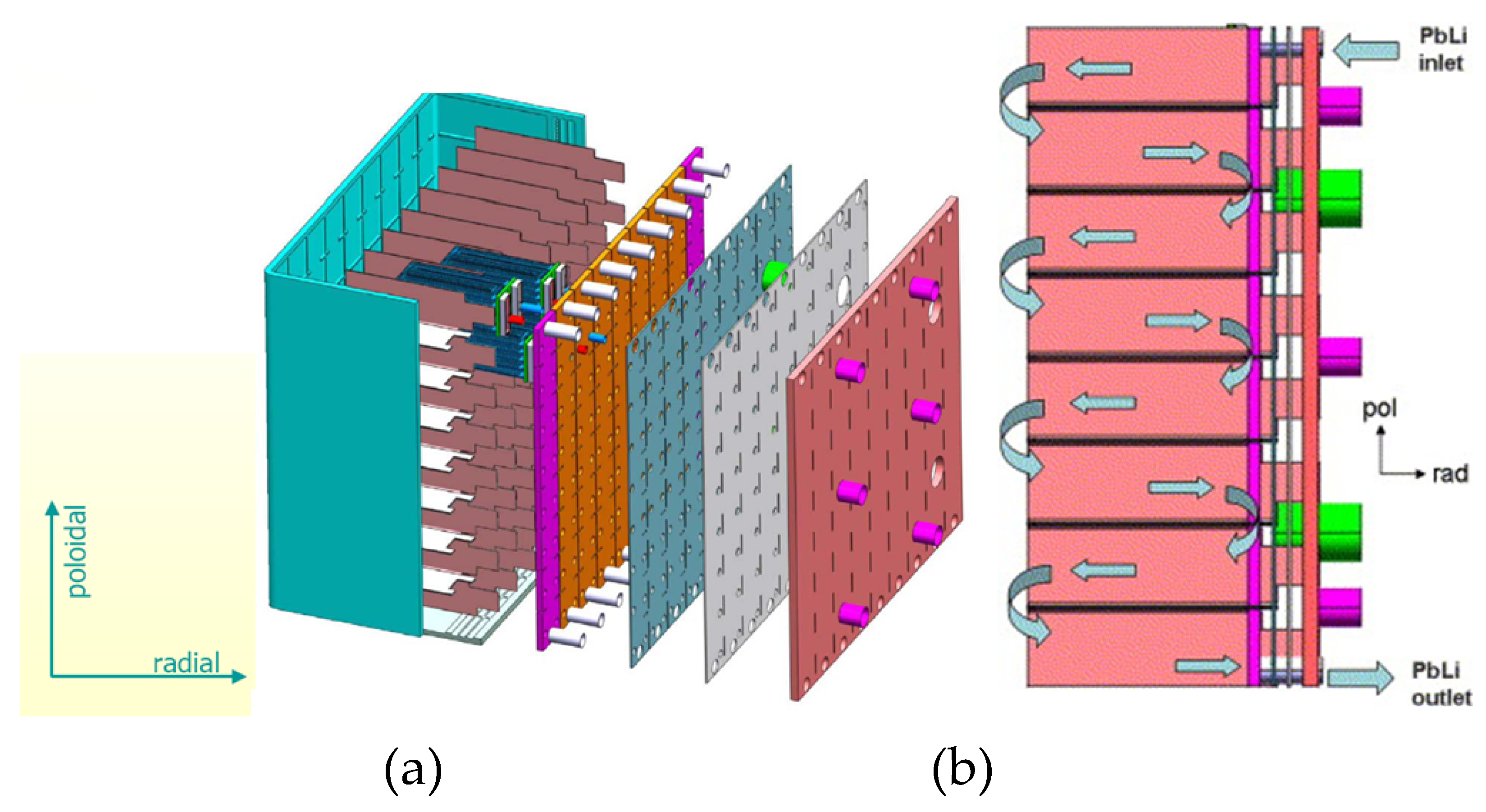
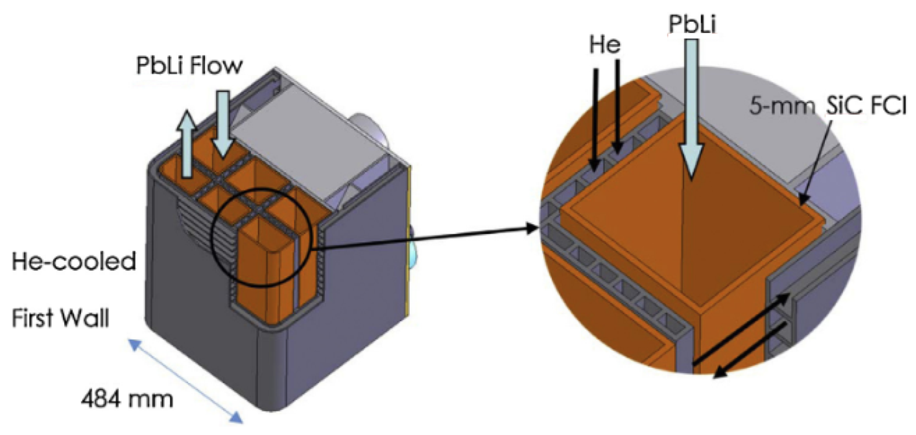
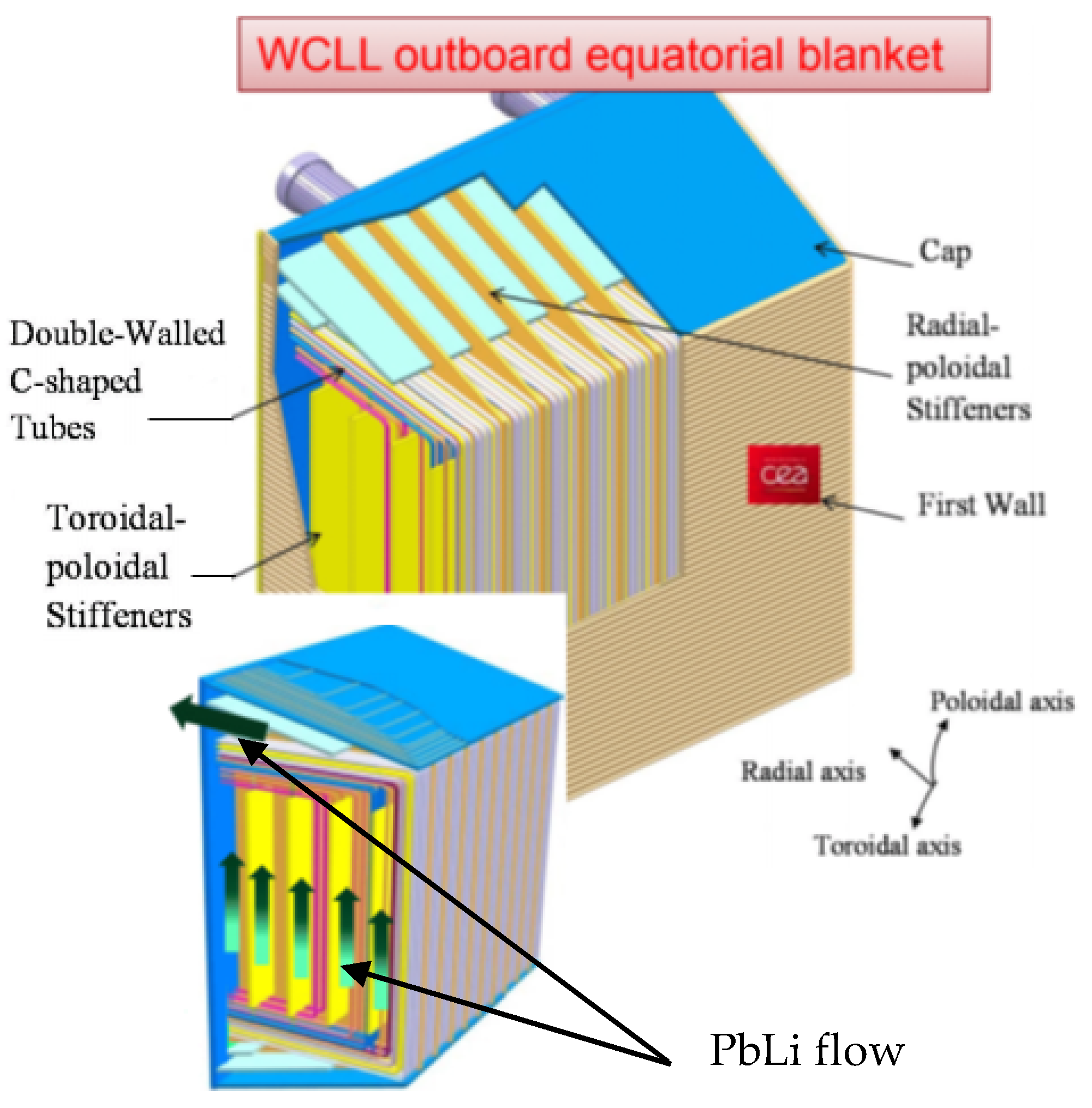
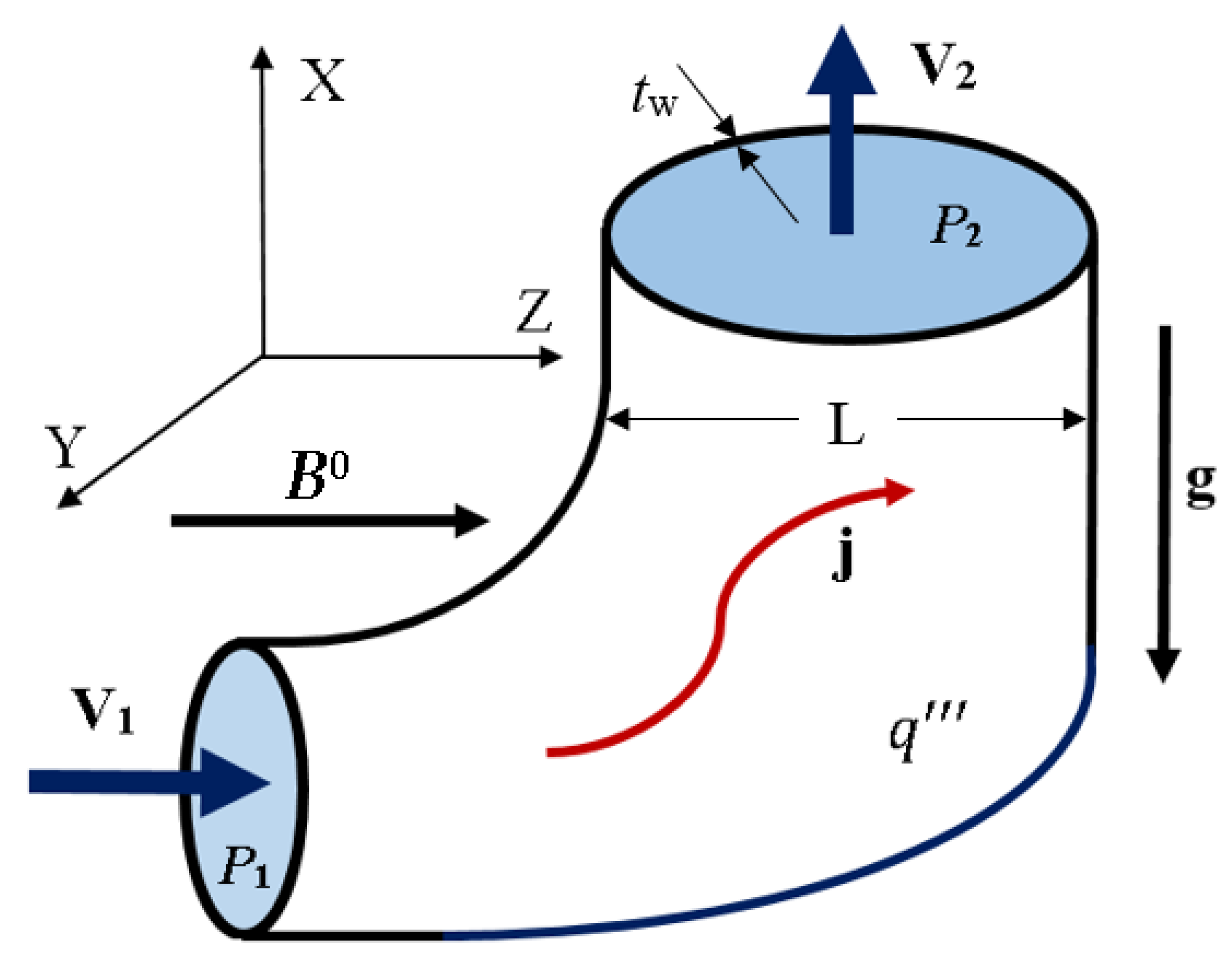
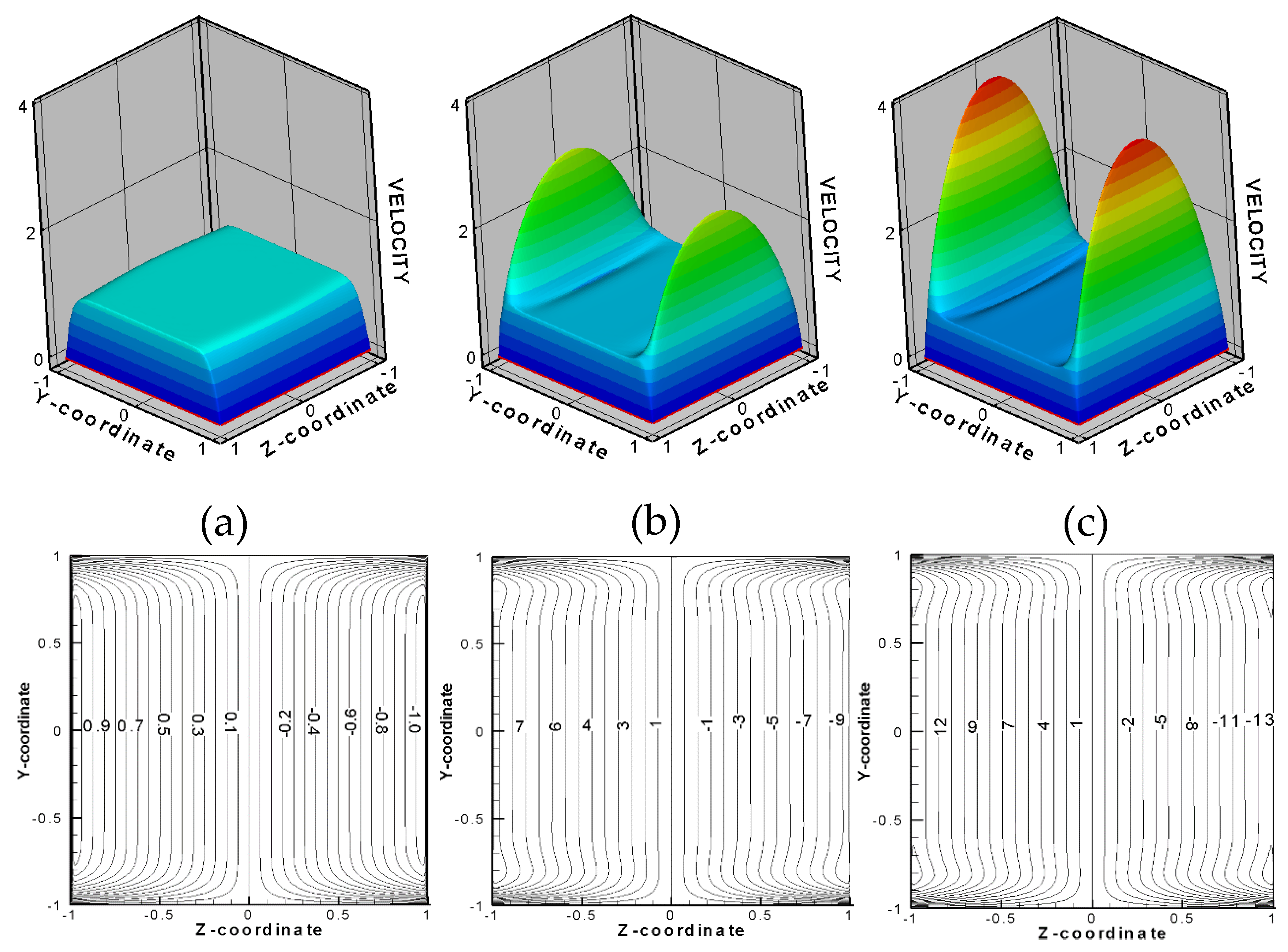
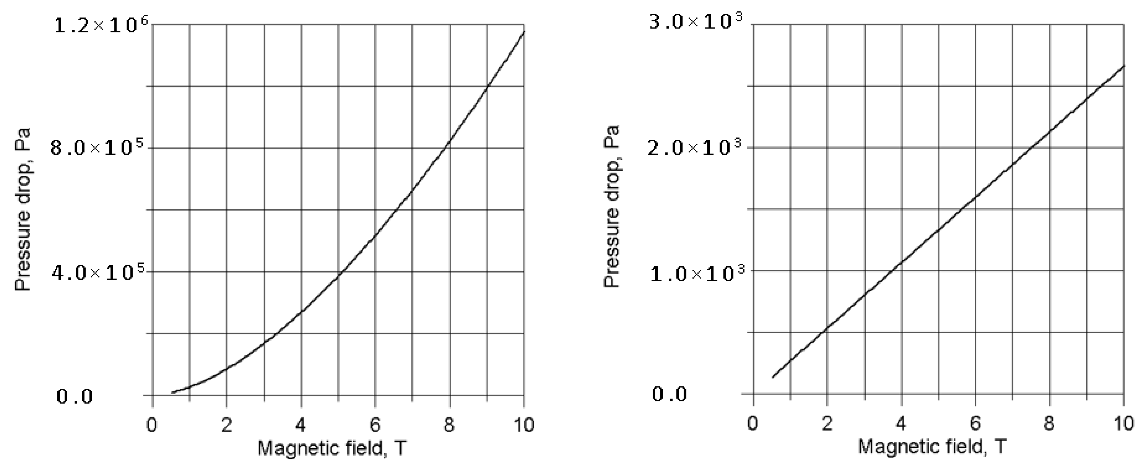
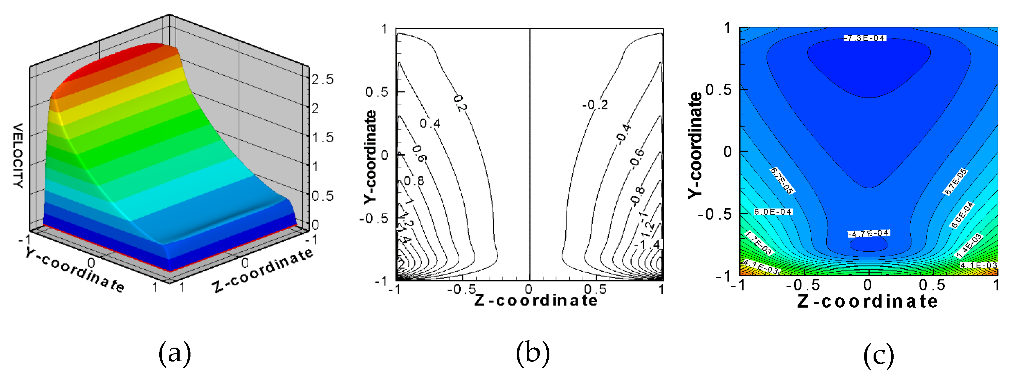
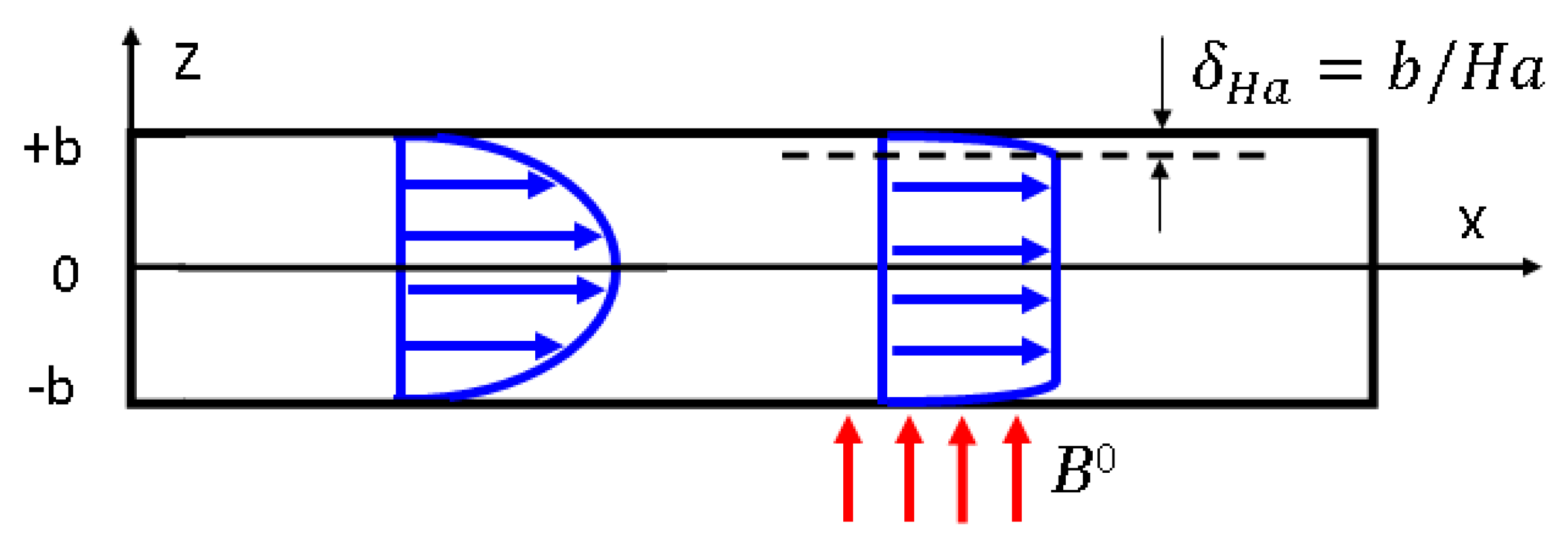
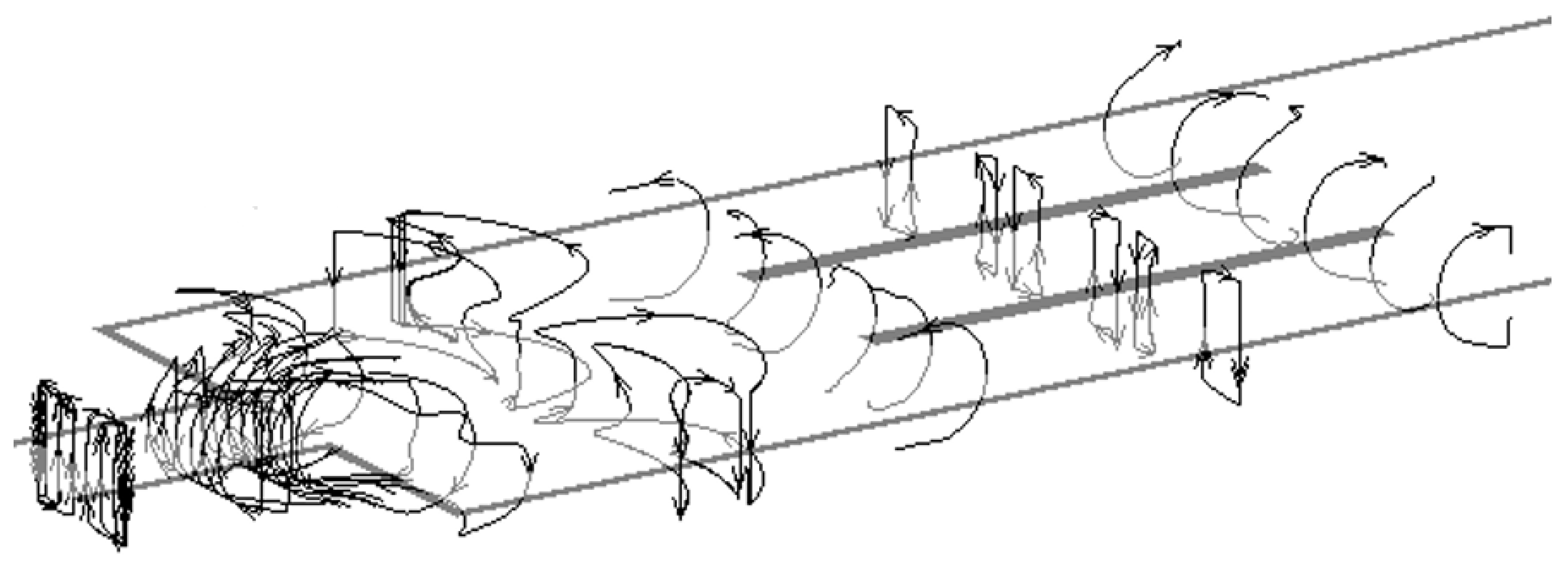
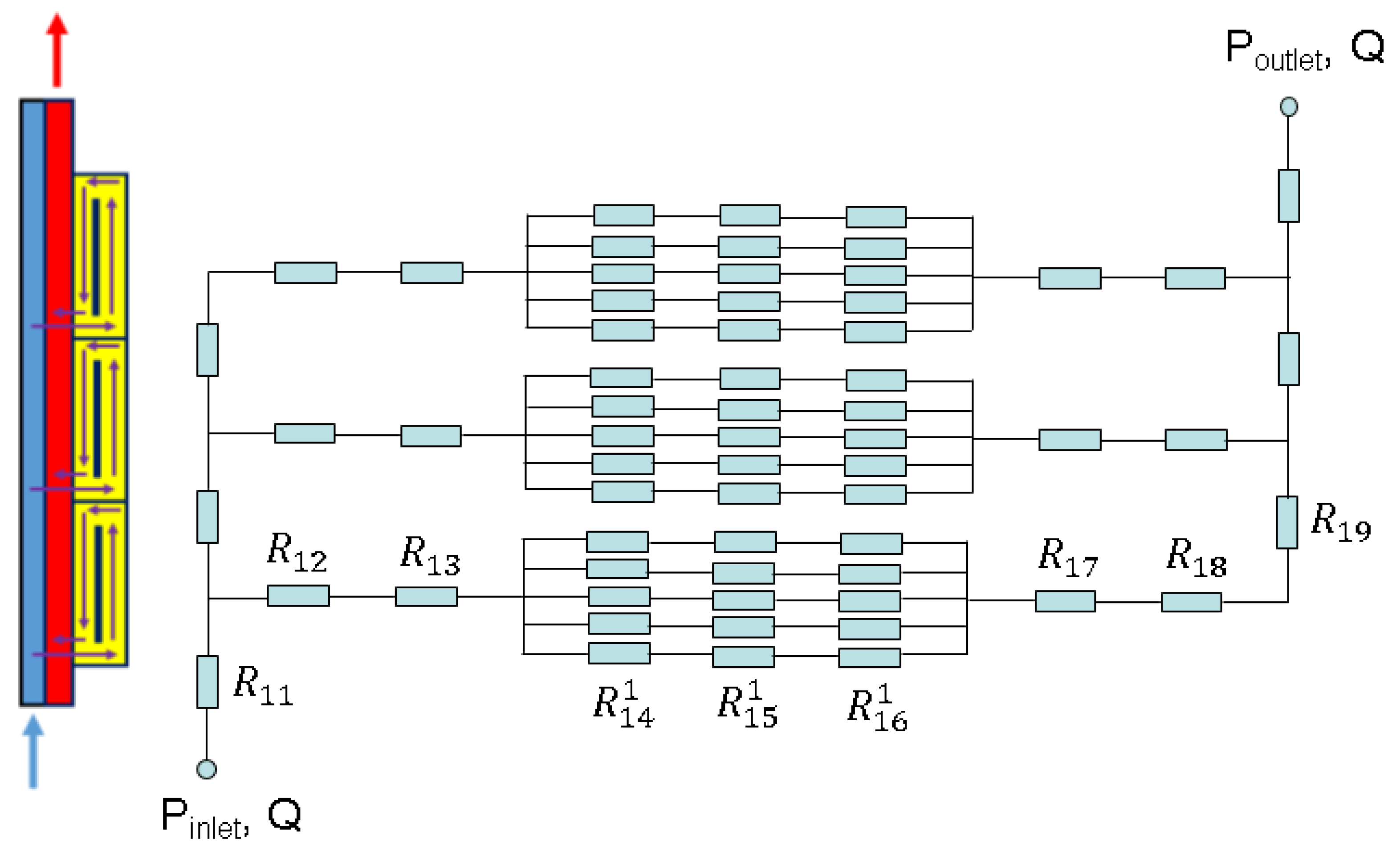
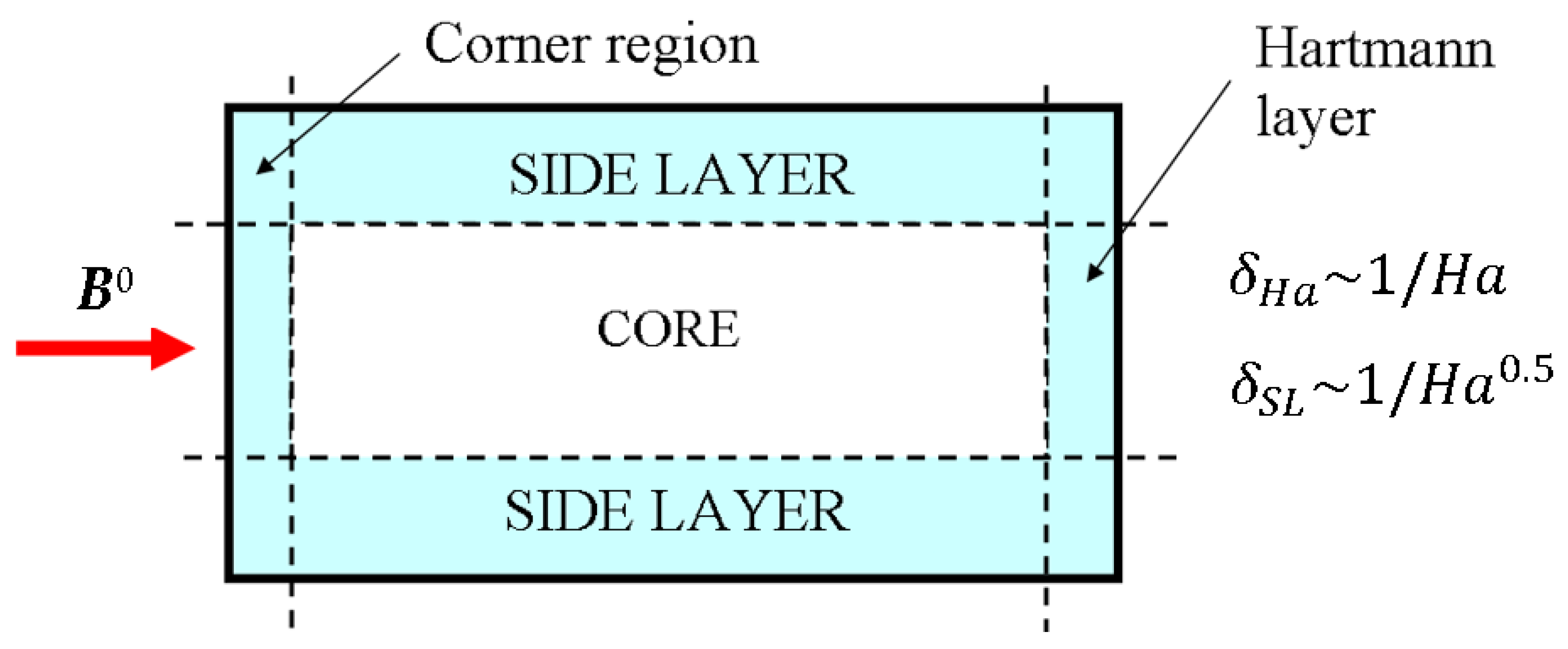
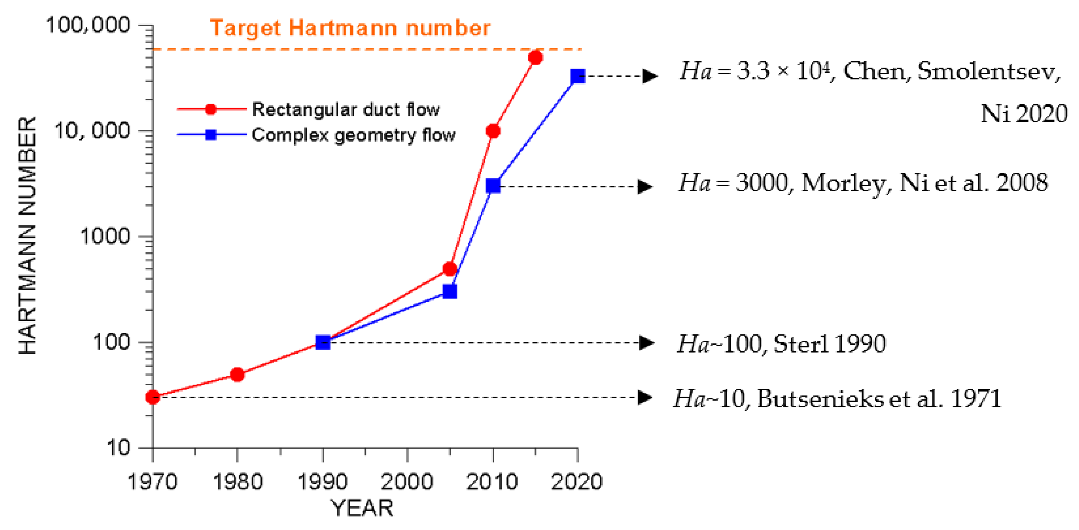
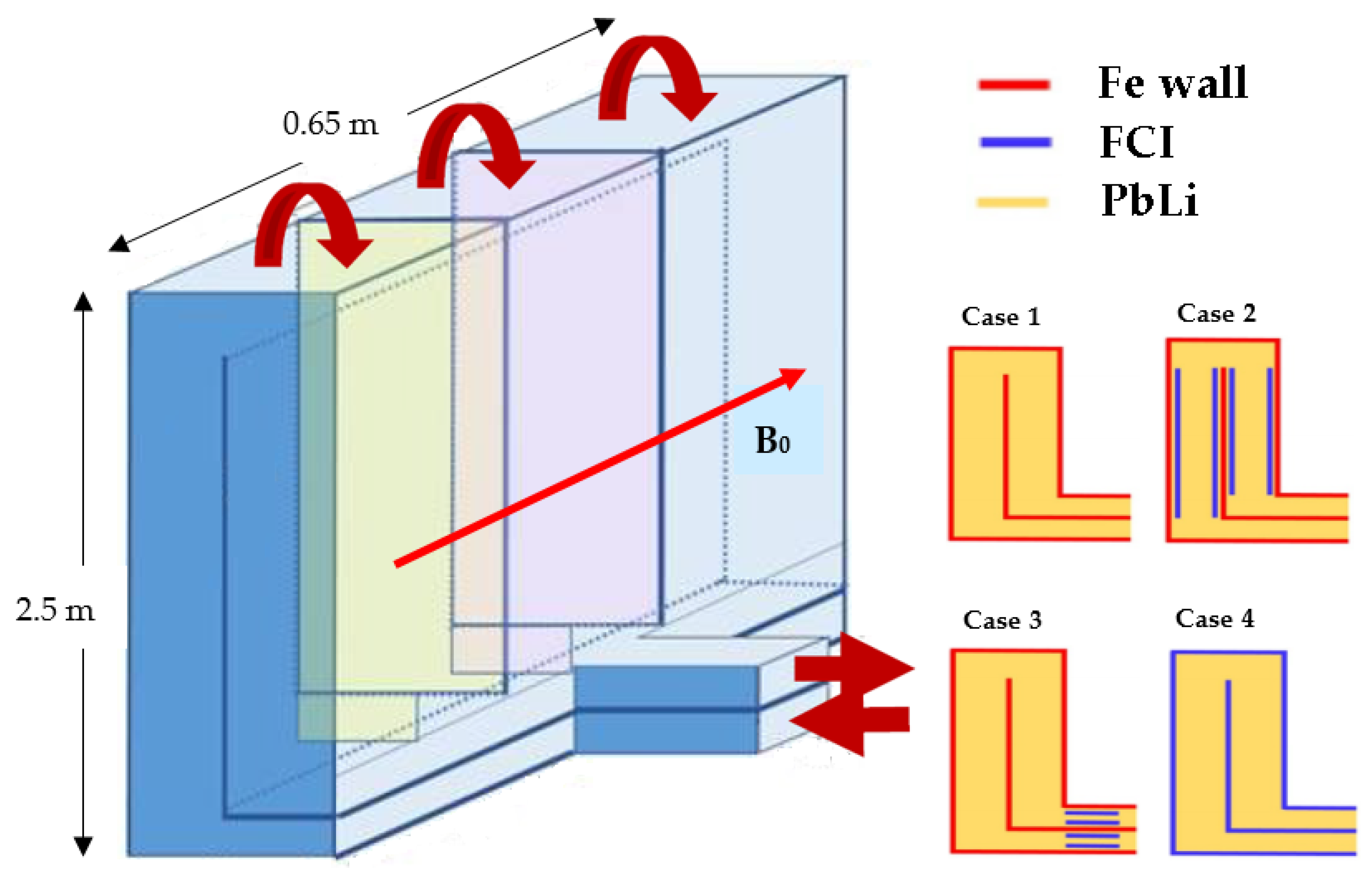
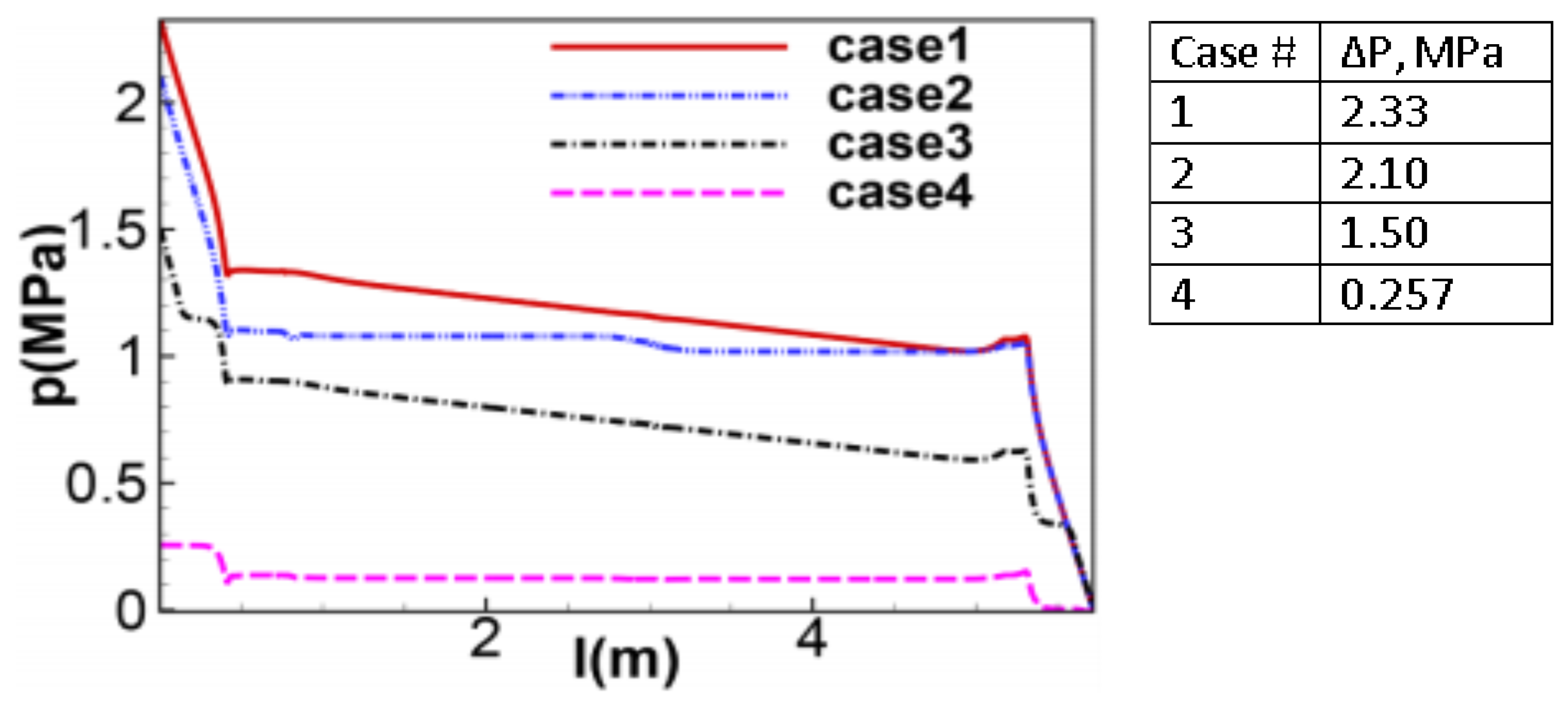
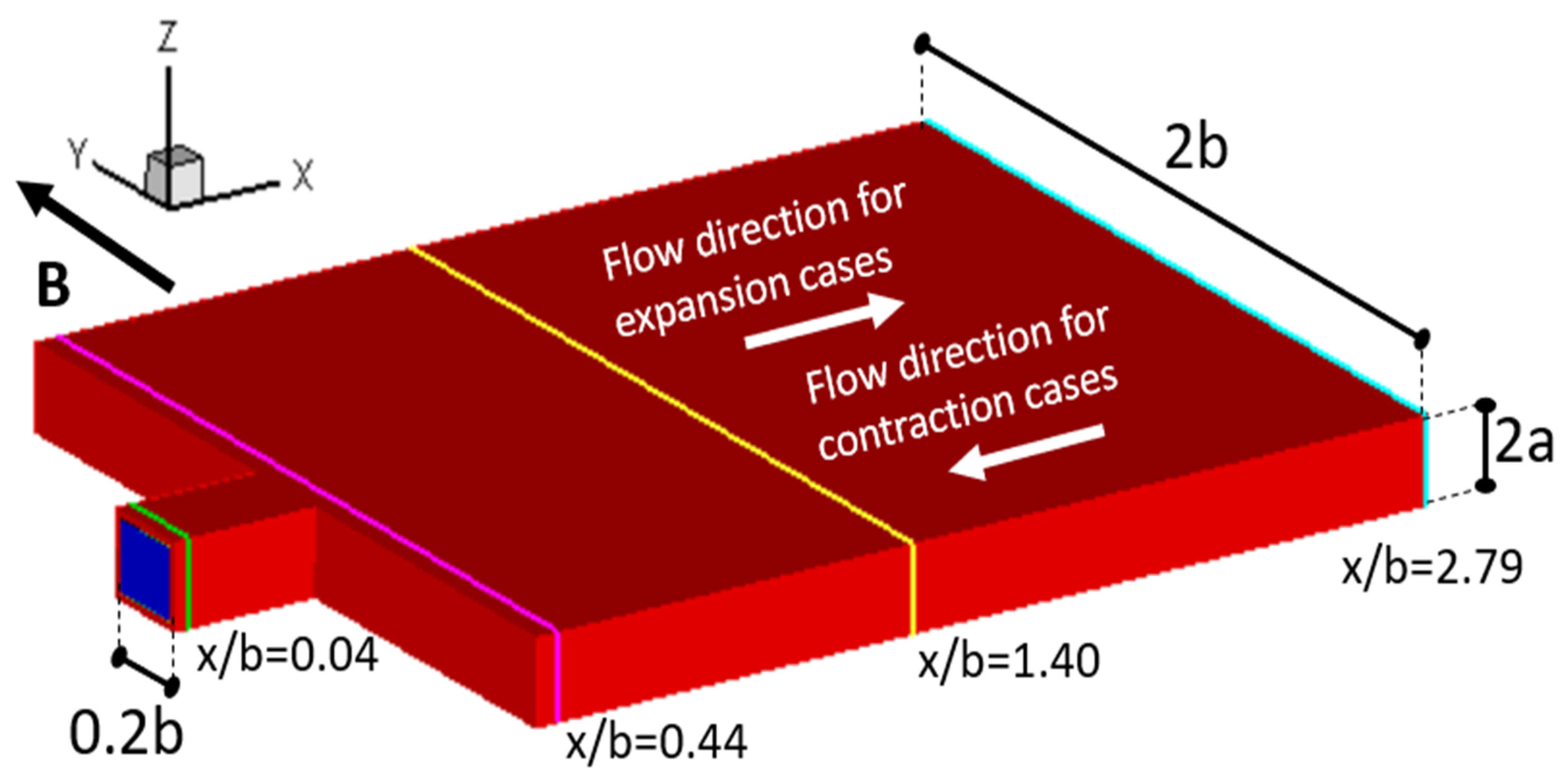
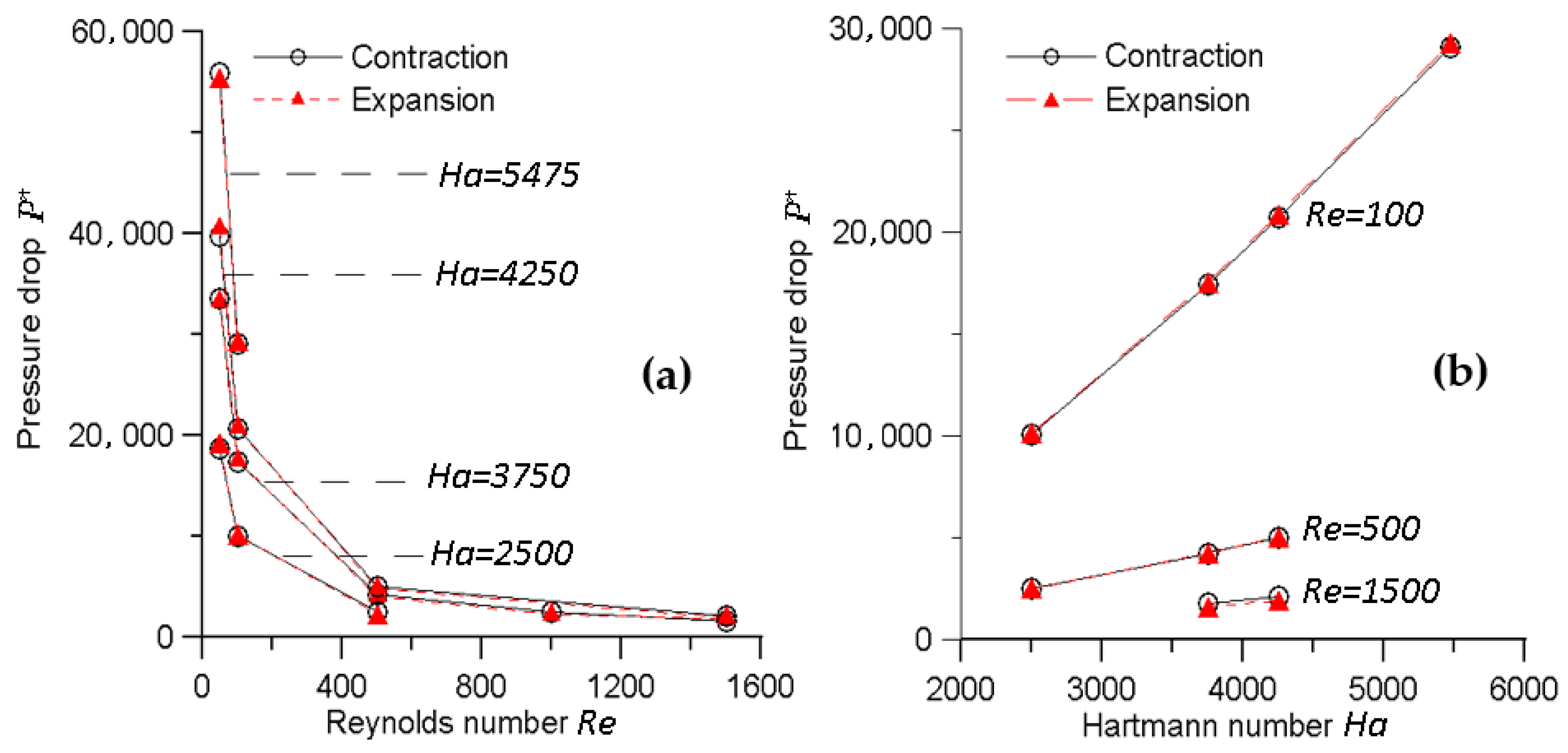
Table 1.
Examples of the dimensionless parameters in several blanket concepts for DEMO, ITER TBM and FNSF, including inboard (IB) and outboard (OB) blankets. Dimensional parameters , , and L are also shown.
Table 1.
Examples of the dimensionless parameters in several blanket concepts for DEMO, ITER TBM and FNSF, including inboard (IB) and outboard (OB) blankets. Dimensional parameters , , and L are also shown.
| Parameter | Li/V Self-Cooled, DEMO IB [3] | HCLL, ITER TBM OB [27] | DCLL, FNSF IB/OB [21] | WCLL, DEMO OB [18] |
|---|---|---|---|---|
| Ha | 4.5 × 10⁴ | 1.1 × 10⁴ | 3.7 × 10⁴/1.5 × 104 | 9.8 × 10³ |
| Re | 3.2 × 10⁴ | 670 | 7.5 × 10⁴/1.7 × 105 | 120 |
| Gr | 6.0 × 10⁸ | 1.0 × 10⁹ | 6.6 × 10¹¹/1.0 × 1012 | 5.4 × 10¹¹ |
| N | 6.0 × 10⁴ | 1.8 × 10⁵ | 1.8 × 10⁴/1.3 × 103 | 8.0 × 10⁵ |
| , T | 10 | 4 | 10/5.5 | 4 |
| , m/s | 0.5 | 0.001 | 0.087/0.203 | 0.0002 |
| L, m | 0.05 | 0.07 | 0.152/0.109 | 0.117 |
Publisher’s Note: MDPI stays neutral with regard to jurisdictional claims in published maps and institutional affiliations. |
© 2021 by the author. Licensee MDPI, Basel, Switzerland. This article is an open access article distributed under the terms and conditions of the Creative Commons Attribution (CC BY) license (http://creativecommons.org/licenses/by/4.0/).
Share and Cite
MDPI and ACS Style
Smolentsev, S. Physical Background, Computations and Practical Issues of the Magnetohydrodynamic Pressure Drop in a Fusion Liquid Metal Blanket. Fluids 2021, 6, 110. https://doi.org/10.3390/fluids6030110
AMA Style
Smolentsev S. Physical Background, Computations and Practical Issues of the Magnetohydrodynamic Pressure Drop in a Fusion Liquid Metal Blanket. Fluids. 2021; 6(3):110. https://doi.org/10.3390/fluids6030110
Chicago/Turabian StyleSmolentsev, Sergey. 2021. "Physical Background, Computations and Practical Issues of the Magnetohydrodynamic Pressure Drop in a Fusion Liquid Metal Blanket" Fluids 6, no. 3: 110. https://doi.org/10.3390/fluids6030110