Risk Assessment Uncertainties in Cybersecurity Investments


1
Institute for Security Science and Technology, Imperial College London, London SW7 2AZ, UK
2
Center for Digital Safety & Security, Austrian Institute of Technology, 1210 Vienna, Austria
3
Surrey Centre for Cyber Security, University of Surrey, Guildford, Surrey GU2 7XH, UK
4
System Security Group, Institute of Applied Informatics, Universität Klagenfurt, 9020 Klagenfurt, Austria
*
Author to whom correspondence should be addressed.
Games 2018, 9(2), 34; https://doi.org/10.3390/g9020034
Submission received: 11 May 2018
/
Revised: 3 June 2018
/
Accepted: 6 June 2018
/
Published: 9 June 2018
(This article belongs to the Special Issue Game Models for Cyber-Physical Infrastructures)
Abstract
:When undertaking cybersecurity risk assessments, it is important to be able to assign numeric values to metrics to compute the final expected loss that represents the risk that an organization is exposed to due to cyber threats. Even if risk assessment is motivated by real-world observations and data, there is always a high chance of assigning inaccurate values due to different uncertainties involved (e.g., evolving threat landscape, human errors) and the natural difficulty of quantifying risk. Existing models empower organizations to compute optimal cybersecurity strategies given their financial constraints, i.e., available cybersecurity budget. Further, a general game-theoretic model with uncertain payoffs (probability-distribution-valued payoffs) shows that such uncertainty can be incorporated in the game-theoretic model by allowing payoffs to be random. This paper extends previous work in the field to tackle uncertainties in risk assessment that affect cybersecurity investments. The findings from simulated examples indicate that although uncertainties in cybersecurity risk assessment lead, on average, to different cybersecurity strategies, they do not play a significant role in the final expected loss of the organization when utilising a game-theoretic model and methodology to derive these strategies. The model determines robust defending strategies even when knowledge regarding risk assessment values is not accurate. As a result, it is possible to show that the cybersecurity investments’ tool is capable of providing effective decision support.
1. Introduction
Many organizations do not have a solid foundation for effective information security risk management. As a result, the increasingly evolving threat landscape in combination with the lack of appropriate cybersecurity defences pose several and important risks. On the other hand, the implementation of optimal cybersecurity strategies (i.e., formal information security processes, technical mechanisms and organizational measures) is not a straightforward process. In particular, Small and Medium Enterprises (SMEs) are a priority focus sector for governments’ economic policy. Given that the majority of SMEs are restricted by limited budgets for investing in cybersecurity, the situation becomes cumbersome, as without cybersecurity mechanisms in place, they may be significantly impacted by inadvertent attacks on their information systems and networks, leading, in most cases, to devastating business effects.
Issues for SMEs are not only restricted to budgetary limitations. Even if sufficient budgets are available, investing in cybersecurity is still challenging due to the evolving nature of cyber threats that introduce several uncertainties when undertaking cybersecurity risk assessments. In this case, an optimal investment decision made at a single point in time may be proven inefficient in due course due to: (i) exploitation of newly found vulnerabilities that were not patched by the latest investment and/or (ii) mistaken values assigned to risk assessment parameters, which can lead to erroneous optimal cybersecurity strategies.
The purpose of this paper is “to investigate how uncertainties in conducting cybersecurity risk assessment affect cybersecurity investments”. As such, this paper looks to extend previous work in the field [1,2]. In the foundation work, the values considered by the simulated environment were considered completely trustworthy. This meant that the decisions made as the result of the implemented tools would inform decisions made with complete trust. However, the factors surrounding data collection and aspects of subjectivity mean that that data cannot be considered with complete trust.
To compensate for a potential lack of trust in the data gathered, the work has been extended to identify the extent to which the accuracy of the data impacts the outputs of such decision tools. To capture the inaccuracies in the data collection process, we represent the problem as uncertainty in the data. Comparisons are made between the values assuming certainty and those displaying uncertainty. The comparisons are designed to identify the degree to which the variation in the data supplied to a simulation impacts the decisions made by the tools. This is done by replicating a known approach, in this case [2]. The outcomes of simulated trials look at the manner in which the uncertainty impacts the optimal solutions. By looking at the amount of uncertainty needed to change the optimal solutions, it is possible to understand the level to which the use of such tools is applicable to the real world. This is such that a tool that requires little uncertainty to cause large changes in the optimal solutions will be less suited to practical deployment for cybersecurity purposes than those that do not.
Security economics: Security economics is a powerful way of looking at overall system security. This field has been introduced. The driver of the field is the application of economic analysis to information security issues. Such analysis aims at addressing the underlying causes of cybersecurity failures within a system or a network, and it complements pure cybersecurity engineering approaches. By taking into account economic parameters, we can propose cybersecurity strategies that minimize risk exposure of systems and networks. It has been shown that spending more on cybersecurity does not necessarily mean that we achieve higher security levels. This is another key challenge that security economics can tackle. A critical consideration is that cybersecurity decision-makers can benefit from security economics approaches, thus making informed decisions about security. It is also worth noting that many cybersecurity mechanisms (e.g., cryptographic protocols) are used to support business models than manage risk.
Anderson was the first to discuss the economics of security by arguing that most information security problems can be explained more clearly and convincingly using the language of microeconomics [3]. Terms that he used include network externalities, asymmetric information, moral hazard, adverse selection, liability dumping and the tragedy of the commons [3]. The seminal work of Gordon and Loeb presents an economic model that determines the optimal amount to invest to protect a given set of information [4]. This is know as the Gordon–Loeb model, and it considers the vulnerability of the information to a security breach and the potential loss should such a breach occur.
Anderson and Moore investigate the interface between security and sociology and the interactions of security with psychology, both through the psychology-and-economics tradition and in response to phishing attacks [5]. A more technical approach is given by Eeten et al. presenting qualitative empirical research on the incentives of market players when dealing with malware [6]. In the same vein, a recent work by Laszka et al. proposes a game-theoretic model that captures a multi-stage scenario where a sophisticated ransomware attacker attacks an organisation. The authors investigate the decision of companies to invest in backup technologies as part of a contingency plan and the economic incentives to pay a ransom if impacted by an attack [7]. More related work about cybersecurity investments is presented in the following.
Cybersecurity investments: According to a 2017 IBM report [8], despite a decline of 10% in the overall cost of a data breach over previous years to $3.62 million, companies in this year’s study have larger breaches. A study conducted by the Ponemon Institute [9] in 2015 on behalf of the security firm Damballa shows that although businesses spend an average of $1.27 million annually and 395 people-hours each week responding to false alerts, thanks to faulty intelligence and alerts, breaches have actually gone up dramatically in the past three years. There are a number of challenges faced by organizations when it comes to investing in cybersecurity. Most prominent amongst these concerns is the issue that the generation of accurate valuations for performing risk assessment is hindered by a lack of clearly-defined reliable and accountable methods. This is in part due to the complexity of developing holistic methodologies that model organizations’ assets and perform appropriate risks assessments to generate optimal solutions.
In cybersecurity, the landscape is ever changing, and the emergence of new threats and technologies will change the applicability of either the data used to perform the initial risk assessment or the validity of the risk assessment itself. There are also significant psychological obstacles like the fact that cybersecurity costs, unlike other expenses, do not induce an easily identifiable return on investment. Instead, it is a pure protection of existing investments, rather than a method to generate revenue itself.
Additionally, the concept of subjectivity on the evaluation of cyber risk demonstrates a core challenge in understanding what the true value of risk is. At a fundamental level, this is due to personal models and perceptions of risk, which will inform and bias evaluations, leading to uncertainty. Studies have looked at how different experts evaluate and rank issues in cybersecurity scenarios [10]. Psychological factors like personal risk aversion or risk affinity may thus play a crucial role in data collection and also the decision-making process.
The literature on the economics of security is quite rich when it comes to methodologies for investing in cybersecurity [11,12,13,14,15]. In our previous works [1,2], we compared different decision support methodologies for security managers to tackle the challenge of investing in security for SMEs. To undertake the risk assessment of the proposed model, we used fixed values for the payoffs of the players (i.e., defender and attacker). These values were set by using a mapping from the SANScritical security controls [16] combined with the Common Weakness Enumeration (CWE) top 25 software vulnerabilities [17]. The upcoming analysis is based on data published in [18]. Although the use of data from well-known sources made our risk assessment valid and important, this approach ignored the fact that in real-world scenarios, there is a very high amount of uncertainty when setting the payoff values. In fact, even the data used in [1] are just as accurate as the activities undertaken by experts when defining these values. However, such activities are prone to error due to: (i) being subjective to the human experience each time; (ii) the evolving threat landscape that unavoidably dictates new risk assessment values; and (iii) new assets being added to an organization’s environment (i.e., infrastructure), therefore altering the current security posture of the organization.
Decision under uncertainty:As mentioned in the previous section, decision problems often involve uncertainty about the consequences of the potential actions. Currently, state-of-the-art decision support methods in general either ignore this uncertainty or reduce existing information (e.g., by aggregating several values into a single number) to simplify the process. However, such approaches burn much information. In [19], we introduce a game theoretic model where the consequences of actions and the payoffs are indeed random, and consequently, they are described as probability distributions. Even though the full space of probability distributions cannot be ordered, a subset of suitable loss distributions that satisfy a few mild conditions can be totally ordered in a way that agrees with the general intuition of risk minimization. We show that existing algorithms from the case of scalar-valued payoffs can be adapted to the situation of distribution-valued payoffs. In particular, an adaption of the fictitious play algorithm allows the computation of a Nash equilibrium for a zero-sum game. This equilibrium then represents the optimal way to decide among several options such that the chance of maximal loss is minimized. The model is described in more depth and illustrated with an example in [20], and the algorithms are implemented in the free software R [21].
An area where such a framework is particularly useful is risk management. Risk is often assessed by experts and thus depends on many factors, including the risk appetite of the person doing the assessment. Additionally, the effects of actions are rarely deterministic, but rather depend on external influences. Therefore, it is recommended by the German Federal Office of Information Security to do a qualitative risk assessment, which is consistent with our approach. We have applied the framework to model security risks in critical utilities such as a water distribution system in [22]. In this situation, consequences are difficult to predict as consumers are not homogeneous and thus do not act like a single (reasonable) person. Another situation that can be modelled with this generalized game-theoretic approach is that of an Advanced Persistent Threat (APT) [23]. Recently, this type of attack has gained much attention due to major incidents such as Stuxnet [24] or the attack on the Ukrainian power grid [25]. We applied this generalized game-theoretic model of APT attacks to two use cases where the expected loss was estimated either by simulation [26] or expert opinions [27], depending on which source of information was available. Further, the same framework has been used to find optimal protection against malware attacks [28].
2. Proposed Methodology
Our work is inspired by two previous papers [1] and [19] to investigate how uncertainties regarding cybersecurity risk assessment values affect the efficiency of cybersecurity investments that have been built upon game-theoretic and combinatorial optimization techniques (a single-objective multiple choice knapsack-based strategy). These uncertainties are reflected in the payoffs of the organization (henceforth referred to as the defender). Although [1] was proven interesting and validated the U.K.’s government aforesaid advice, it certainly did not account for uncertainties in the payoffs of the defender. In real-world scenarios, defenders almost always operate with incomplete information, and often, a rough estimate on the relative magnitude of known cyber threats is the only information available to the cybersecurity managers. Furthermore, practical security engineers will argue that it is already difficult to obtain detailed information on risk assessment parameters. We envisage that by merging these two approaches, we will be able to offer a decision support tool for cybersecurity investments with increased resiliency against threats facing SMEs. More importantly, our work addresses a wider class of cyber threats than commodity cyber threats, which were investigated in [1]. Although this assumption does not negate the possibility of zero-day vulnerabilities, it removes the expectation that it is in the best interest of either players to invest heavily in order to discover a new vulnerability or to protect the system against it.
2.1. Ambiguity in Risk Assessments
Often, a threat can be mitigated by more than one action. When experts come up with different ways of protecting an asset, the selection should be made for the cheapest to implement, yet most effective action against the threat. The problem is simple, but not easy, as the cost for an action may be well known, but not so for the effectiveness or the risk of the threat. This is where things become necessarily subjective to some extent, since the assessment of a threat’s impact can be done in several ways:
- simulation: if the underlying system dynamics admits a sufficiently accurate description, simulations can run.
- expert interviews: brainstorming and individual interviews usually provide a valuable source of information. Methods like Delphi [29] or other panel data gathering techniques can (and should) be applied, but in most cases, the aforementioned psychological matters will come into play, such as:
- -
- What if only a few experts, up to only a single one, are skilled and willing to utter an opinion about the risk? How would that expert be convinced to take the “personal risk” of saying something that guides the decision-makers into making the wrong move (for which the expert would subsequently be held liable perhaps)?
- -
- On which scale would experts rate the risk? The quality of a subjective estimate may strongly depend on the scale being prescribed. Typically, companies will here define their internal risk ratings on nominal scales with textually-defined meanings that are individual for each security goal. That is, losses of a monetary nature are understood differently compared to losses of reputation, legal implications or others. A “low” risk in financial terms may thus mean a loss up to some fixed amount, while a “low” risk for reputation may mean, say, a loss of up to x% of the customers or market share. Such definitions mostly come in tabular form to help an expert frame his/her opinion in the given terms on the nominal scale, but what if the uncertainty is such that more than one category may fit (at least in the expert’s eyes)?
The latter two issues make the data gathering for risk management difficult in practice, but can be addressed by allowing the experts to provide fuzzy assessments instead of hard statements. The challenge is adapting the decision theory to work with these fuzzy terms, which technically amounts to playing games over uncertain numbers, e.g., distributions.
Example: Suppose an expert thinks that the loss is somewhere between medium and high, but she/he cannot (or does not want to) precisely pin down a number. Why not express the uncertainty as it is, by saying “the losses will be somewhat between 10,000 € and 20,000 €”, admitting that even the upper and lower bounds are not fully certain. It is straightforward to express this by a Gaussian distribution centred in the mean of the two bounds and having a standard deviation such that equals the given range. This corresponds to a 95.45% chance of the interval covering the true loss, leaving a 5.5% residual risk of the bounds being still incorrect. Game theory can be soundly defined to use such a Gaussian density as a direct payoff measure.
2.2. Security Games with Uncertainty
The Cybersecurity Control Games (CSCGs) developed so far [1] do not yet capture this problem sketched in the previous section: a crisp prediction of the efficacy of cybersecurity controls, as well as the values of the various other risk assessment parameters is often not possible. Rather, some intuitive information is available that describes some values as more likely than others. In this paper, we enrich the model recently presented in [1] by considering uncertainty in payoffs of the defender (and of the attacker since we play a zero-sum game) in CSCG. This is a two-stage cybersecurity investments model that supports security managers with decisions regarding the optimal allocation of their financial resources in the presence of uncertainty regarding the different risk assessment values.
For a specific set of targets of the attacker and security controls to be implemented by the defender, our approach to cybersecurity risk assessment consists of two main steps. First, a zero-sum CSCG is solved to derive the optimal level at which the control should be implemented to minimize the expected damage if a target is attacked. This game accounts for uncertainty about the effectiveness of a control using the probability distribution as payoffs instead of crisp numbers. As pointed out in Section 1, we show in [19] that imposing some mild restrictions on these distributions admits the construction of a total ordering on a (useful) subset of probability distributions, which allows one to transfer solution concepts like the Nash equilibrium to this new setting.
The most critical part in estimating the damage caused by a cybersecurity attack is predicting the efficacy of a control to protect a target t. Let us assume that we decide to implement the control at some level l; then, we denote the efficacy of the control to protect target t as . Typically, it is difficult to estimate this value, even if l and t are known. Thus, we replace the exact value of by a Gaussian distribution centred around the most likely value with a fixed variance . For simplicity, we assume that the uncertainty is equal for each cybersecurity control and implementation level. This assumption can be relaxed if we have obtained an accurate value about the efficacy of a cybersecurity process (i.e., a control implemented at some level). In order to avoid negative efficacy, we truncate the Gaussian distributions to get a proper probability distribution on . Allowing the efficacy of an implementation of a control at level l on target t to be random yields a random cybersecurity loss . This is the expected damage (e.g., losing some data asset) that the defender suffers when t is attacked and a control has been implemented at level l. This definition of loss is in line with the well-known formula, risk = expected damage × probability of occurrence [30]. We assume that this loss will take values in a compact subset of . The losses in our games are thus random variables, so at this point, we explicitly deviate from the classical route of game theory. In particular, we do not reduce the random payoffs to expected values or similar real-valued representatives. Instead, we will define our games to reward us in terms of a complete probability distribution, which is convenient for several reasons:
- Working with the entire probability distribution preserves all information available for the modeller when the games are defined. In other words, if empirical data or expertise on losses or utilities are available, then condensing them into a humble average sacrifices unnecessarily large amounts of information;
- It equips the modeller with the whole armoury of statistics to define the payoff distribution, instead of forcing the modeller to restrict himself/herself to a “representative value”. The latter is often a practical obstacle, since losses are not always easily quantifiable, nor expressible on numeric scales (for example, if the game is about critical infrastructures and if human lives are at stake, a quantification in terms of “payoff” simply appears inappropriate).
Note that uncertainty in our case is essentially different from the kind of uncertainty that Bayesian or signalling games capture. While the latter is about uncertainty in the opponent, the uncertainty in our case is about the payoff itself. The crucial difference is that Bayesian games nonetheless require a precise modelling of payoffs for all players of all types. This is only practically feasible for a finite number of types (though theoretically not limited to this). In contrast, our games embody an infinitude of different possible outcomes (types of opponents) in a single payoff, thus simplifying the structure of the game back into a standard matrix game, while offering an increased level of generality over Bayesian or signalling games.
In CSCG (a matrix game), the defender and attacker have finite pure strategy spaces (where ) and a payoff structure of the defender, denoted by , which in light of the uncertainties intrinsic to cybersecurity risk assessment, is a matrix of random variables. During the game-play, each player takes his/her actions at random, which determines a row and column for the payoff distribution . Repeating the game, each round delivers a different random payoff , the distribution of which is conditional on the chosen scenario . Thus, we obtain the function . By playing mixed strategies, the distribution of the overall expected random payoff R is obtained from the law of total probability by:
when are the mixed strategies supported on and the player’s moves are stochastically independent (e.g., no signalling).
Unlike classical repeated games, where a mixed strategy is chosen to optimize a long-run average revenue, Equation (1) optimizes the distribution , which is the same (identical) for every repetition of the game. The game is in that sense static, but (unlike its conventional counterpart) does not induce repetitions in practice, since the payoffs are random (in each round), but all having the same distribution. Thus, the “distribution-valued payoff” is always the same (whether there are repetitions of the game or not).
2.3. Cybersecurity Investments and Uncertainty
When having c cybersecurity controls, our plan for cyber investment is to solve c CSCGs by splitting each of them up into a set of control subgames with n targets and up to implementation levels for each control, where (we set to indicate that the control is not implemented at all). For a CSCG, the control subgame equilibria constitute the CSCG solution [1]. Given the control subgame equilibria, we then use a knapsack algorithm to provide the general investment solution. The equilibria provide us with information regarding the way in which each security control is best implemented, so as to maximize the benefit of the control with regard to both ’s strategy and the indirect costs of the organization. For convenience, we denote the control subgame solution by the maximum level of implementation available. For instance, for control , the solution of control subgame is denoted by . Let us assume that for control j, the equilibria of all control subgames are given by the set . For each control, there exists a unique control subgame solution , which dictates that control j should not be used.
We define an optimal solution to the knapsack problem as . A solution takes exactly one solution (i.e., equilibrium or cybersecurity plan) for each control as a policy for implementation. To represent the cybersecurity investment problem, we need to expand the definitions for both expected damage S and effectiveness E to incorporate the control subgame solutions. Hence, we expand S such that , which is the expected damage on target t given the implementation of . Likewise, we expand the definition of the effectiveness of the implemented solution on a given target as . Additionally, we consider as the direct cost of implementing . If we represent the solution by the bit-vector , we can then represent the 0-1 multiple choice, multi-objective knapsack problem as presented in (2).
where B is the available cybersecurity budget, and when . In addition, we consider a tie-break condition in which if multiple solutions are viable, in terms of maximizing the minimum, according to the above function, we will select the solution with the lowest cost. This ensures that an organization is not advised to spend more on security than would produce the same net effect. In Figure 1, we have illustrated the overview of the methodology followed to provide optimal cybersecurity advice supporting decision-makers in deciding about optimal cybersecurity investments.
3. Experiments
In order to reason about the impact of uncertainty on cybersecurity investment decisions, experiments were run to see how the optimal decision would change in the event of uncertainty. The results presented here represent the outcomes of experiments run using a test case comprised of a sample of 10 controls and 20 vulnerabilities from [18].
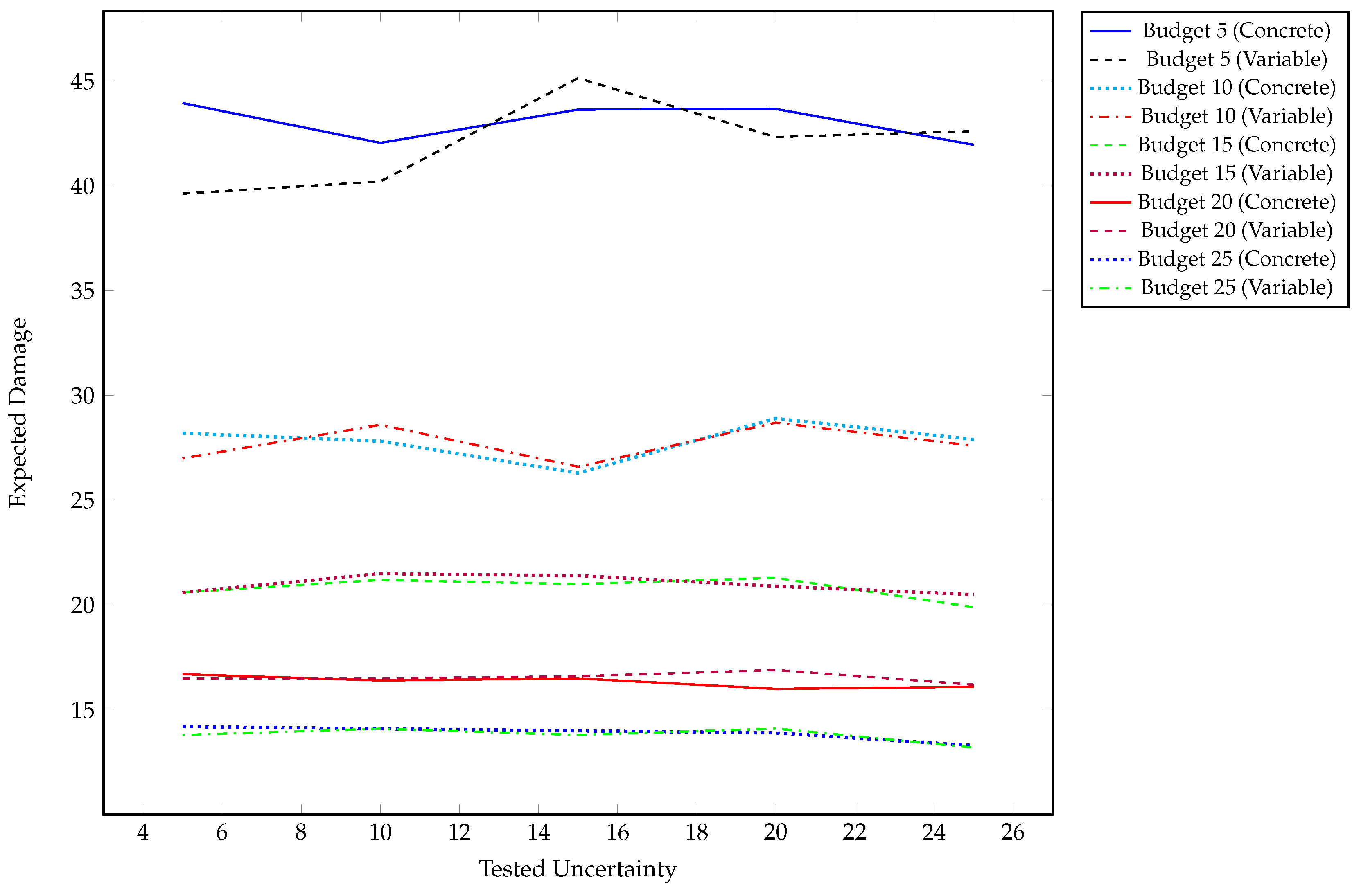
A set of different levels of uncertainty is applied across a range of available budgets, consistent with the methodology presented in [1]. All the reported results are collected in Figure 2, and the expected damage is defined as a normalized value between 0 and 100. For each budget and uncertainty level, 300 simulations were run based on a proposed distribution of attacks for testing the optimal solutions, with the averages presented in Figure 2. Taking this approach leads to aspects of the diversity seen in the expected damage for each of the solutions for the constant values. This measure is predominantly used to identify how different amounts of uncertainty impact the reachability of optimal solutions and, if so, how that would manifest itself in terms of potential damage. Outside of the lowest budget levels tested, the range in expected damage is small.
The tables of this section present the best strategies seen at each budget level when tested with different levels of uncertainty. The number represents the optimal level that a control should be implemented at, where 1 dictates the simplest possible configuration, 5 dictates the best, but most restrictive possible configuration, and 0 represents no implementation of the control. The uncertainty is modelled by a Gaussian distribution, centred at the predicted damage or efficiency value. The variance of that distribution is taken as a percentage fraction of its mean value (e.g., 5%, 10%, …, in Table 1, Table 2 and Table 3).
Budget 5: The expected damage is distributed primarily between 35 and 45. The large range of damage exists because there are few solutions that provide both good coverage and fall within the budget. With a lack of viable solutions, the possibility of covering every vulnerability in some manner diminishes. This lack of coverage means that there is likely to be greater discrepancies in the reported evaluation for possible solutions. Given that the tested solutions at lower levels of uncertainty are the same, the discrepancies are related to the inherent variance in the testing method.
The lack of available budget makes the discovery of optimal solutions more difficult. This is given that the closer the direct cost of a solution tends towards the budget, the more likely the solution under uncertainty will exceed the budget. When this occurs, there is a penalty for the solution. This means that having a heavily constrained budget will minimise the pool of solutions.
We see in Table 1a that all optimal solutions tend towards implementing only two controls. With uncertainty greater than 0.2, we see the same controls, but a different solution. In this case, the first control is implemented at a lower level, while the third control is implemented at a higher level. This represents the notion that Controls 1 and 3 are suited to reducing the most pressing vulnerabilities, but the degree to which one is considered more valuable is dependent on the level of certainty in the data.
Budget 10: We see that the average expected damage falls in the range of 26–29, which is half the range seen for Budget 5. With more controls available, the expected damage should go down; however, at the same time, we see that the solutions become more consistent. The standard deviation is less than 2.5, with a difference in means that never exceeds 2. This represents more consistency in security, given that there is better coverage of vulnerabilities by adding additional controls.
Table 1b shows that the optimal results for Budget 10 build on the basic pattern from those at Budget 5, suggesting implementations for both Controls 1 and 3 regardless of the level of uncertainty. This is consistent with the idea that Controls 1 and 3 both impact the most pressing vulnerabilities. This represents that this pair of controls offers the most cost-effective strategy of covering network vulnerabilities.
With low uncertainty, Control 9 is considered optimal, but at higher levels of uncertainty, Controls 7 and 10 are considered optimal. This means that the optimisation algorithm can identify that there is a set of controls that are consistently effective at providing the desired security, while the additional controls benefit those vulnerabilities where the expected damage is similar. Essentially, there are a number of viable solutions for protecting the system with a budget of 10, all of which can offer similar overall protection, but the most optimal solution is dependant on the variance.
Budget 15: For a budget of 15, we see that the mean expected damage is between 19 and 22. At this budget and higher, we see that the difference in means between the certain and uncertain solutions never exceeds 1.
With the increased budget over the previous results, the optimal solution in Table 2a now always considers a combination of the first three controls. The rest of the budget is used to sporadically patch the worst remaining vulnerabilities as dictated by uncertainty. This means that at lower levels of uncertainty, Control 4 is preferred, while at higher levels of uncertainty, we see that Control 10 becomes the favoured addition to the base set of controls, with Control 9 preferred at 10% uncertainty.
Interestingly, between an uncertainty of 20% and 25%, Control 3 is used at a higher level, where the rest of the solutions remains the same. This indicates that in the latter case, the uncertainty in the values means that there is scope for using a control that might otherwise be out of budget. Given that uncertainty around the cost of implementation is considered, the variance in the valuation made the solution viable.
Budget 20: The range of average expected damage is limited to less than 1, with the biggest discrepancy between the certain and uncertain solution at the 20% uncertainty level.
The optimal solutions from Table 2b add little to the general pattern of solutions that preceded it, implementing the first 3 controls at varying levels. This is the only time that we see the optimal solution suggest the highest level of implementation for Control 1. Here, Control 10 is preferred at lower levels of uncertainty. At higher levels, this and Control 4 are replaced by a combination of Controls 7 and 8.
One commonality between budgets of 15 and 20 is that Control 4 is only considered when there is more certainty in the data. The combination of Controls 2, 4, 9 and 10 identifies the overlap in coverage for certain vulnerabilities. This identifies where uncertainty can impact the optimal solution. Since all four controls cover the same set of vulnerabilities, the uncertainty in the costs and efficiencies will dominate which of those are most effective in any given scenario.
Budget 25: Considering the highest budget tested, we see that the average expected damage has a range of 1, between 13.2 and 14.2. This results in a difference in means of at most 0.4 and a minimum of 0.025. This is combined with standard deviations of no greater than 1.2 to provide consistent results between certain and uncertain solutions.
From Table 3a, the main difference in solutions is that Control 4 becomes a permanent suggestion for implementation in addition to the other 3 core controls. Up to 20% uncertainty, we see some variation of 6 controls, with consistent solutions up to 10% uncertainty and a common solution at 15% and 20% uncertainty. At 25% uncertainty, we see that the optimal solution deviates away from those solutions below. As with all of the results, despite a different solution, we still see a similar expected damage with the solution created in a certain space. With uncertainty and a wide range of available configurations, it is reasonable to consider that there will be a number of solutions that offer similar results. Given that it still shares common factors, we can consider that most of the mitigation is handled by those four controls. The mitigation of the additional controls covers the change in values caused by uncertainty; this is similar to the case seen at 15% uncertainty.
4. Discussion
This section highlights a number of common themes across the results, considering the expected results, as well as themes consistent with the optimal solutions.
Across all of the results in Figure 2, we see only a small difference in mean expected damage between the optimal results with certain and uncertain parameters. This is represented by a difference in the mean values of comparable results not exceeding one standard deviation. While some of the consistency is due to multiple evaluations of solutions, the nature of the designs of the solutions similarly reduces the impact. The hybrid optimization approach requires multiple different negative perturbations on values to be offset by positive perturbations on other controls before the impact will be seen. The value suggested by the expected damage captures these differences in the deviation of the results from the mean.
The optimal results demonstrate a number of changes to the investment strategy as the uncertainty increases. This change can be explained as a combination of the factors that are uncertain. In general, this will be as a result of some controls becoming more effective than others at similar tasks. Less common results will have optimal solutions that might not be considered valid under a certain set of parameters, but based on uncertainty in the costs, would appear to be genuine. It is with this last point that we find one of the sources for deviation in the average expected damage seen in the previous section. Above, we discuss having potentially invalid solutions seen to be optimal, but we also need to consider the case where the most optimal solution was eliminated due to potentially having a cost that would exceed the budget.
Uncertainty in the cost is represented most prominently in the results at low budgets. This is due to the number of viable solutions that can be tested, since most solutions will exceed the budget. With this, the search space for solutions features more local optima, with less coherent strategies for traversal. The consistency in the results can be explained by the coverage of certain controls and their effectiveness at completing that task. Across all the results displayed in Table 1 and Table 2, we see that Control 1 is always selected, and with some limited exceptions, so is Control 3. This gives us an impact on multiple vulnerabilities tested, causing a reduction in the expected damage. It is only at higher budgets that we see that the impact of multiple controls better filling the role of Control 3 causes it to be replaced in the optimal solutions.
In addition to the idea that we see consistent results across low levels of uncertainty, we also see that the results identify that although there are a number of differences in the precise optimal solution, there is commonality among all of the optimal solutions present. The trial was performed with a small set of attacks and controls. Increasing the number of controls and vulnerabilities could increase the potential for less consistent solutions, due to more overlap of controls. Regardless of the composition, good coverage of attack vectors is achieved as the optimal set of controls will always aim to mitigate the most expected damage across all targets.
A desired outcome of the experimental work was to see the extent of the commonality of optimal solutions for each of the levels of uncertainty. As has been explained above, we see that there are a number of commonalities, especially at the same budget levels. Table 3b shows the minimal set of controls and levels that are implemented regardless of the uncertainty. In comparison to the optimal results for each of the budget levels, we see that these share common features on the first three controls and later Control 4. These controls provide a base coverage of the attack vectors, as described previously. The worst-performing base is that of Budget 10, which reflects that of Budget 5; this is due to the deviation between low uncertainty and high uncertainty solutions.
If we consider the justification for the commonality in the representation of different controls, we identify that Control 1 covers half of the vulnerabilities tested to some degree. At the highest level, it has an efficiency of 0.95 on 7 of those vulnerabilities and 0.5 on the rest. With a high efficiency on a wide variety of targets, this identifies why it is a logical component of all optimal solutions. Furthermore, for its cost value, there are no combinations of controls that can offer the same coverage. Based on both cost and efficiency, the coverage provided by Control 1 exceeds that of both Controls 5 and 6, which is why they never appear in the solution space. This means that even though there may be uncertainty about aspects of the performance across the test, the uncertainty was never enough to justify a shift in optimal controls. However, the uncertainty did result in a shift between the level for which the control was selected.
The other common control amongst solutions is Control 3. Control 3 is an inexpensive control that offers good protection against a number of vulnerabilities that Control 1 does not cover. The only other control that covers a similar range of targets is Control 8. We see at the Budget 25 level that there are cases where Control 3 is used at a lower level, but in this case, there is not a reduction in the coverage, as Control 8 performs that task. The number of successful attacks would not be expected to exceed 5% in any case, reducing to under 1% in the cases of using Control 8, as well. The issue is whether the reduction is worthwhile under uncertainty when combining changes in efficiency and cost.
The vulnerabilities that are not covered by Controls 1 and 3 are effectively covered by the remaining controls. In this space, we see that Controls 9 and 10 are utilised at low budget levels, where 2 and 4 are preferred consistently at higher levels. This is due to lower efficiencies of Controls 9 and 10 versus 2 and 4. However, to cover the same vulnerabilities as either Controls 9 or 10, the solution requires both Controls 2 and 4, which is infeasible at lower budgets.
Regarding Controls 9 and 10, they appeared to be used interchangeably in most cases. For these two controls, the optimality of one over the other comes almost completely from uncertainty, with both controls having similar base efficiencies. This highlights another fact of optimisation of investments in cybersecurity, in that there are often multiple ways to cover the same vulnerability. Both aspects of uncertainty in data collection and the business continuity context might define which control works most effectively for the company, but overall, it is more important to know that the vulnerability is covered by some control and that the risk is effectively managed.
From the cybersecurity perspective, we consider that there are sets of advice such as the U.K.’s Cyber Essentials that promote a number of controls. These pieces of advice suggest a set of controls that is reasonable to implement regardless of the degree of complexity or available budget. The base solutions shown here offer the same approach, demonstrating what a solution should contain based on a constrained budget and uncertainty. These base solutions should be taken as a reference point for building secure systems, with decisions made regarding company-specific requirements.
5. Conclusions and Future Work
This work extended previous work published in the field of decision support for cybersecurity. It has demonstrated an approach to cybersecurity investments under uncertainty, where a previous risk assessment-based model was extended for this purpose. To explore this, a series of experiments looking at optimal cybersecurity investments under uncertainty was performed. Uncertainty is naturally a challenge that all cybersecurity managers face when they have to make decisions. The derivation of exact values for various risk assessment parameters seems like an impossible task. Our work here highlights that even with some uncertainty in factors that impact payoffs and viable strategies, there is consistency in the outcomes, where the majority of damage was being mitigated by only a few cybersecurity controls. Although we have concluded about a set of numerical results that clearly demonstrate the benefit of our model and methodology, the expected extension of this work would be to apply the proposed tools to a full realistic case study, allowing for a comparison to expert judgements, capturing where and how the uncertainty arises.
Author Contributions
Conceptualization, A.F., S.K. and E.P.; Methodology, S.S. and S.R.; Software, A.F. and S.K.; Formal Analysis, S.K. and E.P.; Writing—Original Draft Preparation, A.F., S.K. and E.P.; Writing—Review & Editing, S.S., S.K. and S.R.
Conflicts of Interest
The authors declare no conflict of interest.
References
- Fielder, A.; Panaousis, E.; Malacaria, P.; Hankin, C.; Smeraldi, F. Decision support approaches for cybersecurity investment. Decis. Support Syst. 2016, 86, 13–23. [Google Scholar] [CrossRef]
- Panaousis, E.; Fielder, A.; Malacaria, P.; Hankin, C.; Smeraldi, F. Cybersecurity Games and Investments: A Decision Support Approach. In Decision and Game Theory for Security; Springer: Berlin/Heidelberg, Germany, 2014; pp. 266–286. [Google Scholar]
- Anderson, R. Why information security is hard-an economic perspective. In Proceedings of the Seventeenth Annual Computer Security Applications Conference, New Orleans, LA, USA, 10–14 December 2001; pp. 358–365. [Google Scholar]
- Gordon, L.A.; Loeb, M.P. The economics of information security investment. ACM Trans. Inf. Syst. Secur. 2002, 5, 438–457. [Google Scholar] [CrossRef]
- Anderson, R.; Moore, T. Information security economics–and beyond. In Proceedings of the 27th Annual International Cryptology Conference, Santa Barbara, CA, USA, 19–23 August 2007; Springer: Berlin/Heidelberg, Germany, 2007; pp. 68–91. [Google Scholar]
- Van Eeten, M.J.; Bauer, J.M. Economics of Malware: Security Decisions, Incentives and Externalities; OECD Science, Technology and Industry Working Papers; OECD Publishing: Paris, France, 2008. [Google Scholar]
- Laszka, A.; Farhang, S.; Grossklags, J. On the Economics of Ransomware. In Proceedings of the 8th International Conference, GameSec 2017, Vienna, Austria, 23–25 October 2017; Springer: Berlin/Heidelberg, Germany, 2017; pp. 397–417. [Google Scholar]
- Ponemon Institute LLC. Cost of Data Breach Study; Technical Report; Ponemon Institute LLC: Traverse City, MI, USA, 2017. [Google Scholar]
- Ponemon Institute LLC. The Cost of Malware Containment; Technical Report; Ponemon Institute LLC: Traverse City, MI, USA, 2015. [Google Scholar]
- Miller, S.; Wagner, C.; Aickelin, U.; Garibaldi, J.M. Modelling cyber-security experts’ decision making processes using aggregation operators. Comput. Secur. 2016, 62, 229–245. [Google Scholar] [CrossRef]
- Lee, Y.J.; Kauffman, R.J.; Sougstad, R. Profit-maximizing firm investments in customer information security. Decis. Support Syst. 2011, 51, 904–920. [Google Scholar] [CrossRef]
- Chronopoulos, M.; Panaousis, E.; Grossklags, J. An Options Approach to Cybersecurity Investment. IEEE Access 2017, 6. [Google Scholar] [CrossRef]
- Benaroch, M. Real Options Models for Proactive Uncertainty-Reducing Mitigations and Applications in Cybersecurity Investment Decision-Making. Inf. Syst. Res. 2017. [Google Scholar] [CrossRef]
- Gordon, L.A.; Loeb, M.P.; Lucyshyn, W.; Zhou, L. Increasing cybersecurity investments in private sector firms. J. Cybersecur. 2015, 1, 3–17. [Google Scholar] [CrossRef] [Green Version]
- Moore, T.; Dynes, S.; Chang, F.R. Identifying how Firms Manage Cybersecurity Investment; University of California: Berkeley, CA, USA, 2016. [Google Scholar]
- SANS. The Critical Security Controls for Effective Cyber Defense (Version 5.0). Available online: http://www.counciloncybersecurity.org/attachments/article/12/CSC-MASTER-VER50-2-27-2014.pdf (accessed on 19 December 2015).
- CWE. CWE Top 25 Most Dangerous Software Errors (2011). Available online: http://cwe.mitre.org/top25/ (accessed on 19 December 2015).
- Fielder, A.; Panaousis, E. Decision Support Approaches for Cyber Security Investment: Data for Cyber Essentials Case Study. Available online: http://www.panaousis.com/papers/casestudy.pdf (accessed on 19 December 2017).
- Rass, S.; König, S.; Schauer, S. Uncertainty in Games: Using Probability-Distributions as Payoffs. In Proceedings of the 6th International Conference on Decision and Game Theory for Security, London, UK, 4–5 November 2015; Springer: Berlin/Heidelberg, Germany, 2015; pp. 346–357. [Google Scholar]
- Rass, S.; König, S.; Schauer, S. Decisions with Uncertain Consequences—A Total Ordering on Loss-Distributions. PLoS ONE 2016, 11, e0168583. [Google Scholar] [CrossRef] [PubMed]
- Rass, S.; König, S. R Package ‘HyRiM’: Multicriteria Risk Management Using Zero-Sum Games with Vector-Valued Payoffs That Are Probability Distributions; Austrian Institute of Technology: Vienna, Austria, 2016. [Google Scholar]
- Busby, J.S.; Gouglidis, A.; Rass, S.; König, S. Modelling Security Risk in Critical Utilities: The System at Risk as a Three Player Game and Agent Society. In Proceedings of the 2016 IEEE International Conference on Systems, Man, and Cybernetics (SMC), Budapest, Hungary, 9–12 October 2016; pp. 1758–1763. [Google Scholar]
- Rass, S.; König, S.; Schauer, S. Defending Against Advanced Persistent Threats Using Game-Theory. PLoS ONE 2017, 12, e0168675. [Google Scholar] [CrossRef] [PubMed]
- Karnouskos, S. Stuxnet worm impact on industrial cyber-physical system security. In Proceedings of the IECON 2011—37th Annual Conference of the IEEE Industrial Electronics Society, Melbourne, Australia, 7–10 November 2011; pp. 4490–4494. [Google Scholar]
- E-ISAC. Analysis of the Cyber Attack on the Ukrainian Power Grid; Technical Report; E-ISAC: Washington, DC, USA, 2016. [Google Scholar]
- Alshawish, A.; Abid, M.A.; de Meer, H.; Schauer, S.; König, S.; Gouglidis, A.; Hutchison, D. Protecting Water Utility Networks from Advanced Persistent Threats: A Case Study. In HyRiM; Rass, S., Schauer, S., Eds.; Chapter 6; Springer International Publishing: Berlin/Heidelberg, Germany, 2018. [Google Scholar]
- Gouglidis, A.; König, S.; Green, B.; Schauer, S.; Rossegger, K.; Hutchison, D. Advanced Persistent Threats in Water Utility Networks: A Case Study. In HyRiM; Rass, S., Schauer, S., Eds.; Chapter 13; Springer International Publishing: Berlin/Heidelberg, Germany, 2018. [Google Scholar]
- König, S.; Gouglidis, A.; Green, B.; Schauer, S.; Solar, A. Assessing the Impact of Malware Attacks in Utility Networks. In HyRiM; Rass, S., Schauer, S., Eds.; Chapter 14; Springer International Publishing: Berlin/Heidelberg, Germany, 2018. [Google Scholar]
- Linstone, H.A.; Turoff, M. The Delphi Method; Addison-Wesley: Boston, MA, USA, 1975. [Google Scholar]
- Oppliger, R. Quantitative Risk Analysis in Information Security Management: A Modern Fairy Tale. IEEE Secur. Priv. 2015, 13, 18–21. [Google Scholar] [CrossRef]
Figure 1.
Overview of the cybersecurity investment methodology proposed in [1].
Figure 1.
Overview of the cybersecurity investment methodology proposed in [1].

Figure 2.
Expected damage tracked against uncertainty for each experimental configuration.


Table 1.
Optimal solutions.
| (a) Budget = 5 | ||||||||||
| Uncertainty | 1 | 2 | 3 | 4 | 5 | 6 | 7 | 8 | 9 | 10 |
| 0% | 4 | 0 | 1 | 0 | 0 | 0 | 0 | 0 | 0 | 0 |
| 5% | 4 | 0 | 1 | 0 | 0 | 0 | 0 | 0 | 0 | 0 |
| 10% | 4 | 0 | 1 | 0 | 0 | 0 | 0 | 0 | 0 | 0 |
| 15% | 4 | 0 | 1 | 0 | 0 | 0 | 0 | 0 | 0 | 0 |
| 20% | 3 | 0 | 2 | 0 | 0 | 0 | 0 | 0 | 0 | 0 |
| 25% | 3 | 0 | 2 | 0 | 0 | 0 | 0 | 0 | 0 | 0 |
| (b) Budget = 10 | ||||||||||
| Uncertainty | 1 | 2 | 3 | 4 | 5 | 6 | 7 | 8 | 9 | 10 |
| 0% | 3 | 0 | 1 | 0 | 0 | 0 | 0 | 0 | 4 | 0 |
| 5% | 3 | 0 | 1 | 0 | 0 | 0 | 0 | 0 | 4 | 0 |
| 10% | 3 | 0 | 1 | 0 | 0 | 0 | 0 | 0 | 4 | 0 |
| 15% | 4 | 0 | 3 | 0 | 0 | 0 | 1 | 0 | 0 | 0 |
| 20% | 4 | 0 | 3 | 0 | 0 | 0 | 1 | 0 | 0 | 0 |
| 25% | 4 | 0 | 2 | 0 | 0 | 0 | 0 | 0 | 0 | 2 |
Table 2.
Optimal solutions.
| (a) Budget = 15 | ||||||||||
| Uncertainty | 1 | 2 | 3 | 4 | 5 | 6 | 7 | 8 | 9 | 10 |
| 0% | 4 | 2 | 3 | 1 | 0 | 0 | 0 | 0 | 0 | 0 |
| 5% | 4 | 2 | 3 | 1 | 0 | 0 | 0 | 0 | 0 | 0 |
| 10% | 4 | 2 | 3 | 0 | 0 | 0 | 0 | 0 | 1 | 0 |
| 15% | 4 | 3 | 2 | 0 | 0 | 0 | 0 | 0 | 0 | 1 |
| 20% | 4 | 3 | 2 | 0 | 0 | 0 | 0 | 0 | 0 | 1 |
| 25% | 4 | 3 | 3 | 0 | 0 | 0 | 0 | 0 | 0 | 1 |
| (b) Budget = 20 | ||||||||||
| Uncertainty | 1 | 2 | 3 | 4 | 5 | 6 | 7 | 8 | 9 | 10 |
| 0% | 5 | 3 | 2 | 1 | 0 | 0 | 0 | 0 | 0 | 1 |
| 5% | 5 | 3 | 2 | 1 | 0 | 0 | 0 | 0 | 0 | 1 |
| 10% | 5 | 3 | 2 | 1 | 0 | 0 | 0 | 0 | 0 | 1 |
| 15% | 5 | 4 | 2 | 0 | 0 | 0 | 0 | 1 | 2 | 0 |
| 20% | 5 | 4 | 2 | 0 | 0 | 0 | 0 | 1 | 2 | 0 |
| 25% | 5 | 4 | 3 | 0 | 0 | 0 | 0 | 0 | 3 | 0 |
Table 3.
Solutions.
| (a) Optimal Solutions for Budget 25 | ||||||||||
| Uncertainty | 1 | 2 | 3 | 4 | 5 | 6 | 7 | 8 | 9 | 10 |
| 0% | 4 | 4 | 3 | 3 | 0 | 0 | 0 | 3 | 0 | 0 |
| 5% | 4 | 4 | 3 | 3 | 0 | 0 | 0 | 3 | 0 | 0 |
| 10% | 4 | 4 | 3 | 3 | 0 | 0 | 0 | 3 | 0 | 0 |
| 15% | 4 | 4 | 1 | 3 | 0 | 0 | 0 | 2 | 3 | 0 |
| 20% | 4 | 4 | 1 | 3 | 0 | 0 | 0 | 2 | 3 | 0 |
| 25% | 3 | 2 | 3 | 3 | 0 | 0 | 1 | 0 | 4 | 0 |
| (b) Base Solutions for All Budgets Tested | ||||||||||
| Budget | 1 | 2 | 3 | 4 | 5 | 6 | 7 | 8 | 9 | 10 |
| 5 | 3 | 0 | 1 | 0 | 0 | 0 | 0 | 0 | 0 | 0 |
| 10 | 3 | 0 | 1 | 0 | 0 | 0 | 0 | 0 | 0 | 0 |
| 15 | 4 | 2 | 2 | 0 | 0 | 0 | 0 | 0 | 0 | 0 |
| 20 | 5 | 3 | 2 | 0 | 0 | 0 | 0 | 0 | 0 | 0 |
| 25 | 3 | 2 | 1 | 4 | 0 | 0 | 0 | 0 | 0 | 0 |
© 2018 by the authors. Licensee MDPI, Basel, Switzerland. This article is an open access article distributed under the terms and conditions of the Creative Commons Attribution (CC BY) license (http://creativecommons.org/licenses/by/4.0/).
Share and Cite
MDPI and ACS Style
Fielder, A.; König, S.; Panaousis, E.; Schauer, S.; Rass, S. Risk Assessment Uncertainties in Cybersecurity Investments. Games 2018, 9, 34. https://doi.org/10.3390/g9020034
AMA Style
Fielder A, König S, Panaousis E, Schauer S, Rass S. Risk Assessment Uncertainties in Cybersecurity Investments. Games. 2018; 9(2):34. https://doi.org/10.3390/g9020034
Chicago/Turabian StyleFielder, Andrew, Sandra König, Emmanouil Panaousis, Stefan Schauer, and Stefan Rass. 2018. "Risk Assessment Uncertainties in Cybersecurity Investments" Games 9, no. 2: 34. https://doi.org/10.3390/g9020034
Note that from the first issue of 2016, this journal uses article numbers instead of page numbers. See further details here.