In Situ Block Size Distribution Aimed at the Choice of the Design Block for Rockfall Barriers Design: A Case Study along Gardesana Road

 , ,
, ,  and
and 
Abstract
:1. Introduction
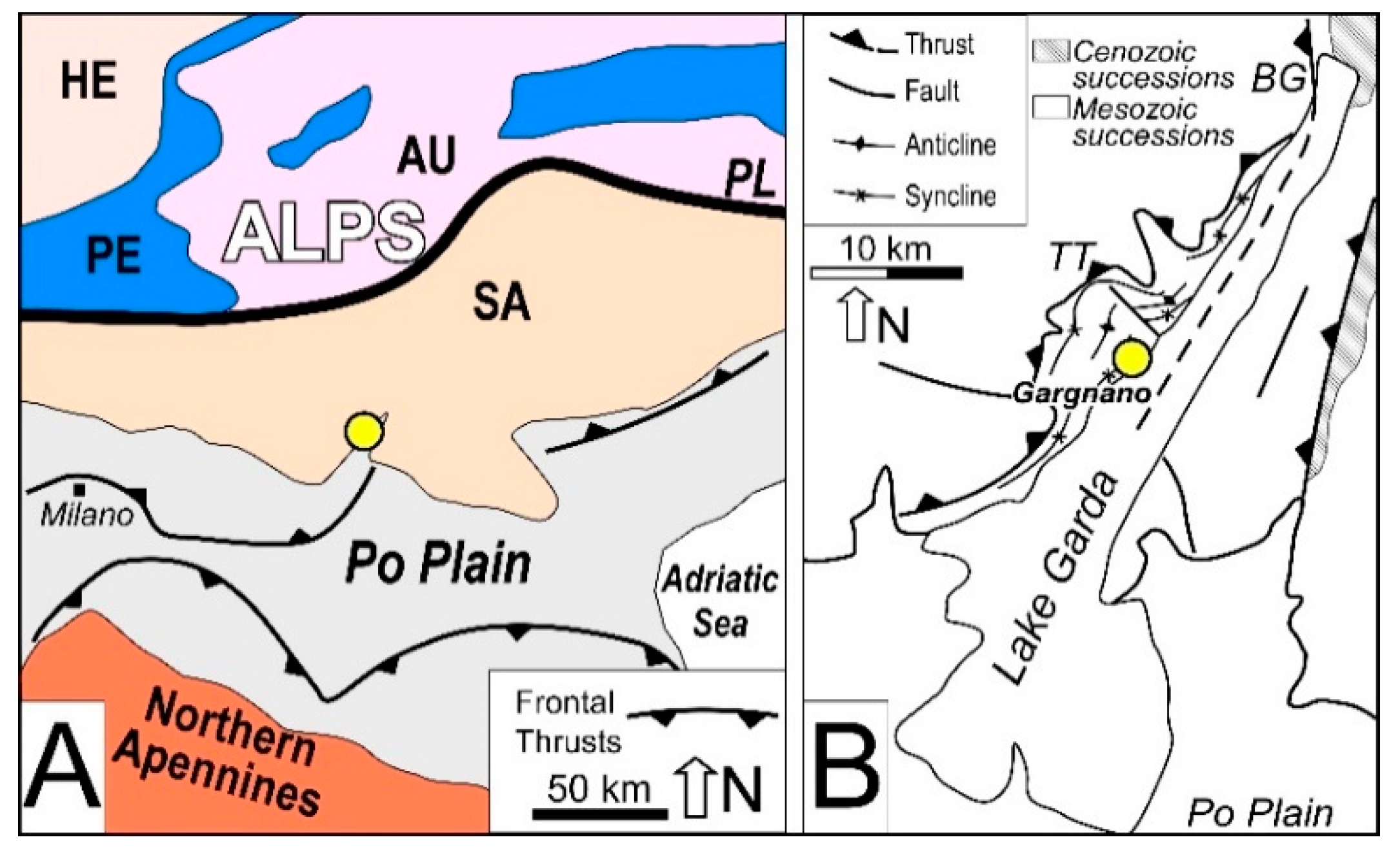
2. Geological Setting
3. Methods
3.1. Block Volume Assessment
3.2. IBSD Assessment
3.2.1. Method Based on Empirical Coefficients
- Determine the principal spacing for the three different sets.
- Determine the three characteristic angles α, β, and ϕ.
- Plot the principle spacing data as histograms and assign the appropriate principal spacing distribution. Hence, determine the principal mean spacing.
3.2.2. Method Based on the Cumulative Distribution Function
3.2.3. Method Based on Monte Carlo Simulation
3.3. Surveys for Block Volume Parameters Definition
3.3.1. Non-Contact Survey
3.3.2. In Situ Traditional Survey
3.4. Blocks Volume Survey at the Foot of the Slope
4. Application to the Case Study
4.1. Traditional Survey
4.2. Non-Contact Survey
5. Discussion
6. Conclusions
Author Contributions
Funding
Acknowledgments
Conflicts of Interest
References
- Hungr, O.; Leroueil, S.; Picarelli, L. The Varnes classification of landslide types, an update. Landslides 2014, 11, 167–194. [Google Scholar] [CrossRef]
- Lambert, C.; Thoeni, K.; Giacomini, A.; Casagrande, D.; Sloan, S. Rockfall hazard analysis from discrete fracture network modelling with finite persistence discontinuities. Rock Mech. Rock Eng. 2012, 45, 871–884. [Google Scholar] [CrossRef]
- Ferrero, A.M.; Migliazza, M.R.; Pirulli, M.; Umili, G. Some open issues on rockfall hazard Analysis in fractured rock mass: Problems and Prospects. Rock Mech. Rock Eng. 2016, 49, 3615–3629. [Google Scholar] [CrossRef]
- Agliardi, F.; Crosta, G.B. High resolution three-dimensional numerical modelling of rockfalls. Int. J. Rock Mech. Min. Sci. 2003, 40, 455–471. [Google Scholar] [CrossRef]
- Lu, P.; Latham, J.-P. Developments in the assessment of In-Situ block size distributions of rock masses. Rock Mech. Rock Eng. 1999, 32, 29–49. [Google Scholar] [CrossRef]
- Wang, L.G.; Yamashita, S.; Sugimoto, F.; Pan, C.; Tan, G. A methodology for predicting the In Situ size and shape distribution of rock blocks. Rock Mech. Rock Eng. 2003, 36, 121–142. [Google Scholar] [CrossRef]
- Wang, H.; Latham, J.-P.; Poole, A. In-Situ block size assessment from discontinuity spacing data. Int. J. Rock Mech. Min. Sci. Geomech. Abstr. 1993, 30, A106. [Google Scholar] [CrossRef]
- Wang, H.; Latham, J.-P.; Poole, A.B. Predictions of block size distribution for quarrying. Q. J. Eng. Geol. Hydrogeol. 1991, 24, 91–99. [Google Scholar] [CrossRef]
- Goodman, R.E.; Shi, G.H. Block Theory and Its Application to Rock Engineering; Prentice Hall Inc.: Englewood Cliffs, NJ, USA, 1985; ISBN 0-t3-078189-4. [Google Scholar]
- Elmouttie, M.K.; Poropat, G.V. A method to estimate In Situ block size distribution. Rock Mech. Rock Eng. 2012, 45, 401–407. [Google Scholar] [CrossRef]
- Stavropoulou, M. Discontinuity frequency and block volume distribution in rock masses. Int. J. Rock Mech. Min. Sci. 2014, 65, 62–74. [Google Scholar] [CrossRef]
- Priest, S.D.; Hudson, J.A. Estimation of discontinuity spacing and trace length using scanline surveys. Int. J. Rock Mech. Min. Sci. Geomech. Abstr. 1981, 18, 183–197. [Google Scholar] [CrossRef]
- Latham, J.-P.; Van Meulen, J.; Dupray, S. Prediction of In-Situ block size distributions with reference to armourstone for breakwaters. Eng. Geol. 2006, 86, 18–36. [Google Scholar] [CrossRef]
- Kemeny, J.; Donovan, J. Rock mass characterisation using LIDAR and automated point cloud processing. Gr. Eng. 2005, 38, 26–29. [Google Scholar]
- Trinks, I.; Clegg, P.; McCaffrey, K.; Jones, R.; Hobbs, R.; Holdsworth, B.; Holliman, N.; Imber, J.; Waggott, S.; Wilson, R. Mapping and analysing virtual outcrops. Vis. Geosci. 2005, 10, 13–19. [Google Scholar] [CrossRef]
- Slob, S.; van Knapen, B.; Hack, R.; Turner, K.; Kemeny, J. Method for automated discontinuity analysis of rock slopes with three-dimensional laser scanning. Transp. Res. Rec. J. Transp. Res. Board 2005, 1913, 187–194. [Google Scholar] [CrossRef]
- Haneberg, W.C. Using close range terrestrial digital photogrammetry for 3-D rock slope modeling and discontinuity mapping in the United States. Bull. Eng. Geol. Environ. 2008, 67, 457–469. [Google Scholar] [CrossRef]
- Ferrero, A.M.; Forlani, G.; Roncella, R.; Voyat, H.I. Advanced geostructural survey methods applied to rock mass characterization. Rock Mech. Rock Eng. 2009, 42, 631–665. [Google Scholar] [CrossRef]
- Sturzenegger, M.; Stead, D. Close-range terrestrial digital photogrammetry and terrestrial laser scanning for discontinuity characterization on rock cuts. Eng. Geol. 2009, 106, 163–182. [Google Scholar] [CrossRef]
- Gigli, G.; Casagli, N. Semi-automatic extraction of rock mass structural data from high resolution LIDAR point clouds. Int. J. Rock Mech. Min. Sci. 2011, 48, 187–198. [Google Scholar] [CrossRef]
- Lato, M.J.; Vöge, M. Automated mapping of rock discontinuities in 3D lidar and photogrammetry models. Int. J. Rock Mech. Min. Sci. 2012, 54, 150–158. [Google Scholar] [CrossRef]
- Vöge, M.; Lato, M.J.; Diederichs, M.S. Automated rockmass discontinuity mapping from 3-dimensional surface data. Eng. Geol. 2013, 164, 155–162. [Google Scholar] [CrossRef]
- Riquelme, A.J.; Abellán, A.; Tomás, R.; Jaboyedoff, M. A new approach for semi-automatic rock mass joints recognition from 3D point clouds. Comput. Geosci. 2014, 68, 38–52. [Google Scholar] [CrossRef] [Green Version]
- Gomes, R.K.; De Oliveira, L.P.L.; Gonzaga, L.; Tognoli, F.M.W.; Veronez, M.R.; De Souza, M.K. An algorithm for automatic detection and orientation estimation of planar structures in LiDAR-scanned outcrops. Comput. Geosci. 2016, 90, 170–178. [Google Scholar] [CrossRef]
- Guo, J.; Liu, S.; Zhang, P.; Wu, L.; Zhou, W.; Yu, Y. Towards semi-automatic rock mass discontinuity orientation and set analysis from 3D point clouds. Comput. Geosci. 2017, 103, 164–172. [Google Scholar] [CrossRef]
- Caselle, C.; Umili, G.; Bonetto, S.; Ferrero, A.M. Application of DIC analysis method to the study of failure initiation in gypsum rocks. Géotech. Lett. 2019, 9, 35–45. [Google Scholar] [CrossRef]
- Sturzenegger, M.; Stead, D.; Elmo, D. Terrestrial remote sensing-based estimation of mean trace length, trace intensity and block size/shape. Eng. Geol. 2011, 119, 96–111. [Google Scholar] [CrossRef]
- Umili, G.; Ferrero, A.; Einstein, H.H. A new method for automatic discontinuity traces sampling on rock mass 3D model. Comput. Geosci. 2013, 51, 182–192. [Google Scholar] [CrossRef]
- Li, X.; Chen, J.; Zhu, H. A new method for automated discontinuity trace mapping on rock mass 3D surface model. Comput. Geosci. 2016, 89, 118–131. [Google Scholar] [CrossRef]
- Riquelme, A.J.; Abellán, A.; Tomás, R. Discontinuity spacing analysis in rock masses using 3D point clouds. Eng. Geol. 2015, 195, 185–195. [Google Scholar] [CrossRef] [Green Version]
- Buyer, A.; Schubert, W. Calculation the spacing of discontinuities from 3D point clouds. Procedia Eng. 2017, 191, 270–278. [Google Scholar] [CrossRef]
- Buyer, A.; Aichinger, S.; Schubert, W. Applying photogrammetry and semi-automated joint mapping for rock mass characterization. Eng. Geol. 2020, 264, 105332. [Google Scholar] [CrossRef]
- Eurocode 7: Geotechnical Design—Part 1: General Rules; EN 1997-1; European Committee for standardization: Brussels, Belgium, 2004.
- Umili, G.; Bonetto, S.; Ferrero, A.M. An integrated multiscale approach for characterization of rock masses subjected to tunnel excavation. J. Rock Mech. Geotech. Eng. 2018, 10, 513–522. [Google Scholar] [CrossRef]
- Ferrero, A.M.; Umili, G.; Migliazza, M.R. Some open issues on the design of protection barriers against rockfall. In Proceedings of the 49th US Rock Mechanics/Geomechanics Symposium 2015, San Francisco, CA, USA, 1–28 July 2015; pp. 3104–3109. [Google Scholar]
- UNI 11211–4. Opere di Difesa Dalla Caduta Massi—Parte 4: Progetto Definitivo ed Esecutivo; UNI: Rome, Italy, 2018. [Google Scholar]
- Technical Protection Against Rockfall—Terms and Definitions, Effects of Actions, Design, Monitoring and Maintenance; ONR 24810; Austrian Standards Institute: Vienna, Austria, 2017.
- Eurocode—Basis of Structural Design; EN 1990:2002+A1; European Committee for standardization: Brussels, Belgium, 2005.
- Vagnon, F.; Ferrero, A.M.; Umili, G.; Segalini, A. A factor strength approach for the design of rock fall and debris flow barriers. Geotech. Geol. Eng. 2017, 35, 2663–2675. [Google Scholar] [CrossRef]
- De Biagi, V.; Lia Napoli, M.; Barbero, M.; Peila, D. Estimation of the return period of rockfall blocks according to their size. Nat. Hazards Earth Syst. Sci. 2017, 17, 103–113. [Google Scholar] [CrossRef] [Green Version]
- Mavrouli, O.; Corominas, J.; Jaboyedoff, M. Size distribution for potentially unstable rock masses and In Situ rock blocks using LIDAR-generated digital elevation models. Rock Mech. Rock Eng. 2015, 48, 1589–1604. [Google Scholar] [CrossRef] [Green Version]
- Dal Piaz, G.V.; Bistacchi, A.; Massironi, M. Geological outline of the Alps. Episodes 2003, 26, 175–180. [Google Scholar] [CrossRef] [Green Version]
- Dal Piaz, G.V. The Italian Alps: A journey across two centuries of Alpine geology. J. Virtual Explor. 2010, 36, 8. [Google Scholar] [CrossRef]
- Bertotti, G.; Picotti, V.; Bernoulli, D.; Castellarin, A. From rifting to drifting: Tectonic evolution of the South-Alpine upper crust from the Triassic to the Early Cretaceous. Sediment. Geol. 1993, 86, 53–57. [Google Scholar] [CrossRef]
- Castellarin, A.; Vai, G.B.; Cantelli, L. The Alpine evolution of the Southern Alps around the Giudicarie faults: A Late Cretaceous to Early Eocene transfer zone. Tectonophysics 2006, 414, 203–223. [Google Scholar] [CrossRef]
- Regione Lombardia. Carta Geologica 1:250,000. Available online: http://www.w3.org/1999/xlink" xlink:href="https://www.cartografia.servizirl.it/viewer32/index.jsp?parameters={‘srsWkid’:32632,‘serviceLMOperator’:‘include’,‘widgetVisible’:‘Gestisci%20contenuto’,‘servicesLM’:[{‘wkid’:32632,‘queryAndZoom’:null,‘servicename’:’’,‘servicehost’:’’,‘type’:‘ESRI:AGSD’,‘label’:‘Carta%20Geologica%20250.000’,‘layerDefinitions’:[],‘visible’:‘true’,‘url’:‘http://www.cartografia.servizirl.it/expo/rest/services/gpt/cartageo_250/MapServer’,‘docuuid’:‘{018208BD-AD82-4D2A-B195-548D6F3432B4}’,‘layerId’:0,‘alpha’:0.7}]} (accessed on 6 May 2020).
- Servizio Geologico d’Italia, 1948–Foglio 35 Riva del Garda della Carta Geologica d’Italia, Scala 1:100,000. Available online: http://193.206.192.231/carta_geologica_italia/tavoletta.php?foglio=35 (accessed on 6 May 2020).
- Regione Lombardia. Gargnano, Piano di Governo del Territorio, Carta Geologica Est. Available online: https://www.multiplan.servizirl.it/pgtweb/pub/pgtweb.jsp (accessed on 6 May 2020).
- Bigi, G.; Cosentino, D.; Parotto, M.; Sartori, R.; Scandone, P. Scientific Coordination and Editing; Structural model of Italy, scale 1:500,000; CNR: Trento, Italy, 1983. [Google Scholar]
- Miles, R.E. The random division of space. Adv. Appl. Probab. 1972, 4, 243–266. [Google Scholar] [CrossRef]
- Palmstrøm, A. Characterizing rock masses by the RMi for use in practical rock engineering. Tunn. Undergr. Sp. Technol. 1996, 11, 175–188. [Google Scholar] [CrossRef]
- Lu, P. The Characterisation and Analysis of In-Situ and Blasted Block Size Distributions and the Blastability of Rock Masses. Ph.D. Thesis, Queen Mary and Westfield College, University of London, London, UK, 1997. [Google Scholar]
- Ferrero, A.M.; Umili, G. Comparison of methods for estimating fracture size and intensity applied to Aiguille Marbrée (Mont Blanc). Int. J. Rock Mech. Min. Sci. 2011, 48, 1262–1270. [Google Scholar] [CrossRef]
- Wang, H. Predictions of In-Situ and Blastpile Block Size Distributions of Rock Masses, with Special Reference to Coastal Requirements. Ph.D. Thesis, Queen Mary and Westfield College, London University, London, UK, 1992. [Google Scholar]
- International Society for Rock Mechanics. ISRM commission on standardization of laboratory and field tests: Suggested methods for the quantitative description of discontinuities in rock masses. Int. J. Rock. Mech. Min. 1978, 15, 319–368. [Google Scholar] [CrossRef]
- Ruiz-Carulla, R.; Corominas, J.; Mavrouli, O. A methodology to obtain the block size distribution of fragmental rockfall deposits. Landslides 2015, 12, 815–825. [Google Scholar] [CrossRef] [Green Version]
- Ruiz-Carulla, R.; Corominas, J.; Mavrouli, O. A fractal fragmentation model for rockfalls. Landslides 2017, 14, 875–889. [Google Scholar] [CrossRef]
- Marchelli, M.; De Biagi, V. Optimization methods for the evaluation of the parameters of a rockfall fractal fragmentation model. Landslides 2019, 16, 1385–1396. [Google Scholar] [CrossRef]


| Passing | Uniform | Negative Exp. | Log-Normal | Fractal | ||||
|---|---|---|---|---|---|---|---|---|
| % | Ci,p | Range | Ci,p | Range | Ci,p | Range | Ci,p | Range |
| 10 | 0.375 | 0.157 | 0.332 | 0.131 | 0.469 | 0.099 | 0.4649 | 0.0128 |
| 20 | 0.700 | 0.292 | 0.710 | 0.249 | 0.965 | 0.207 | 1.1685 | 0.0409 |
| 30 | 1.052 | 0.435 | 1.207 | 0.423 | 1.513 | 0.334 | 2.1606 | 0.0748 |
| 40 | 1.460 | 0.607 | 1.852 | 0.645 | 2.220 | 0.542 | 3.5458 | 0.1612 |
| 50 | 1.939 | 0.787 | 2.708 | 0.984 | 3.099 | 0.731 | 5.3165 | 0.192 |
| 60 | 2.548 | 1.036 | 3.980 | 1.550 | 4.287 | 1.029 | 8.0903 | 0.3098 |
| 70 | 3.343 | 1.384 | 5.867 | 2.596 | 5.956 | 1.501 | 13.3920 | 0.8398 |
| 80 | 4.495 | 1.802 | 8.948 | 4.581 | 8.497 | 2.243 | 22.6070 | 2.2649 |
| 90 | 6.623 | 2.691 | 15.332 | 9.532 | 13.377 | 4.227 | 39.6660 | 5.0295 |
| 100 | 17.772 | 9.348 | 38.992 | 23.734 | 38.277 | 17.569 | 108.9700 | 9.6708 |
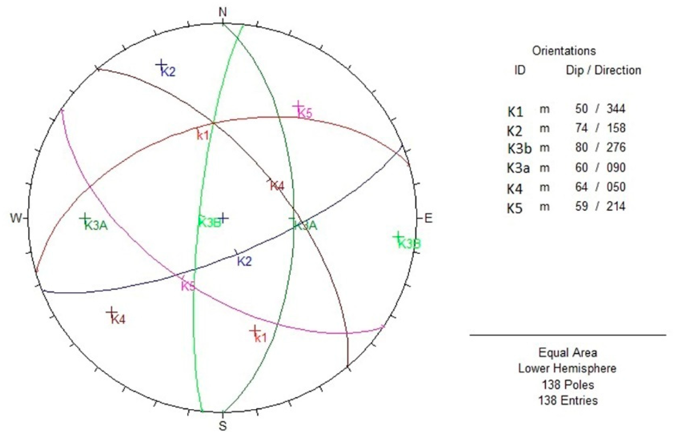
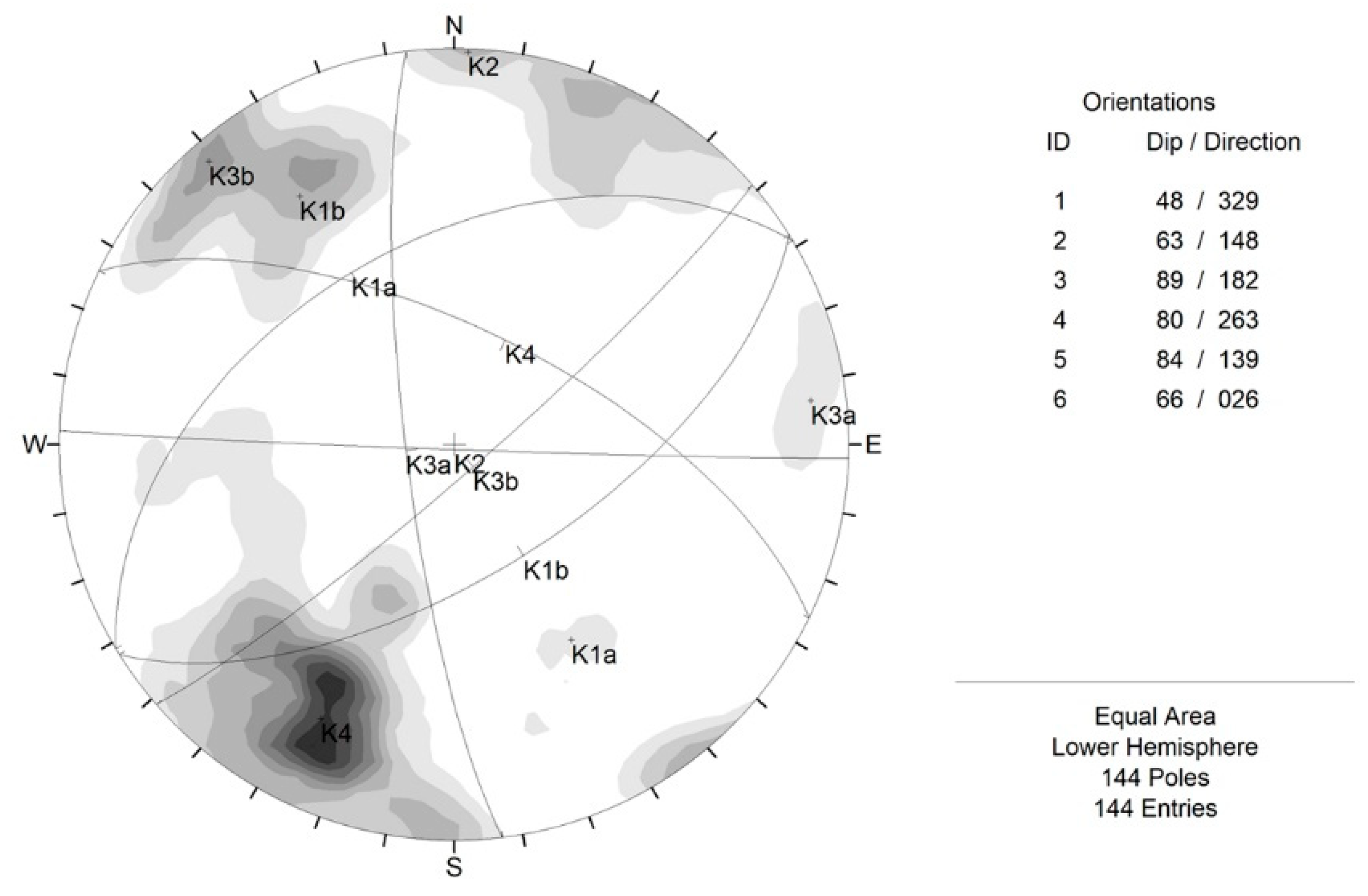
| Set | Dip | Dip Direction | Spacing Range (m) |
|---|---|---|---|
| K1 | 50 | 344 | 0.02–1.55 |
| K2 | 74 | 158 | 0.22–3.38 |
| K3a | 60 | 090 | 0.02–2.88 |
| K3b | 80 | 276 | 0.07–3.44 |
| K4 | 64 | 050 | 0.18–1.86 |
| K5 | 59 | 214 | 0.15–0.96 |
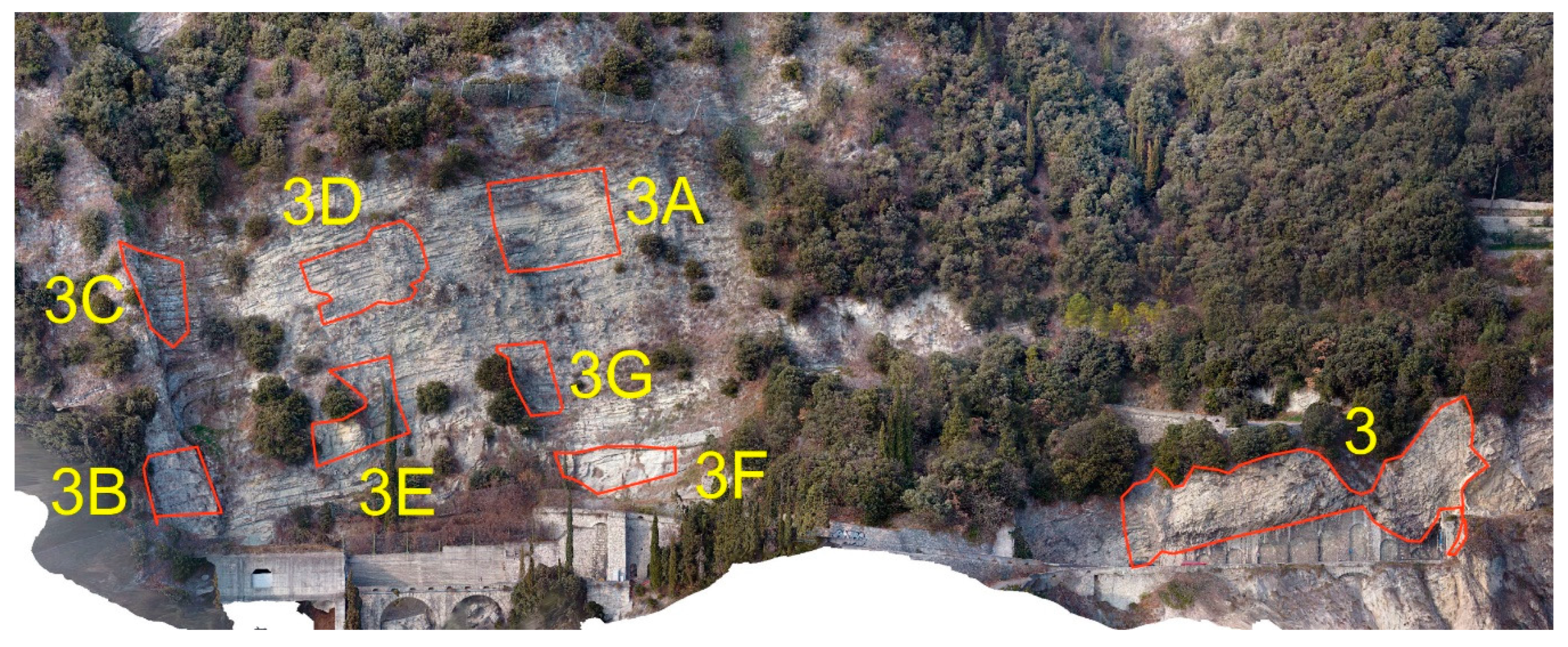
| Window | Number of Discontinuities |
|---|---|
| 3 | 246 |
| 3A | 282 |
| 3B | 192 |
| 3C | 176 |
| 3D | 210 |
| 3E | 146 |
| 3F | 184 |
| 3G | 144 |
| TOTAL | 1580 |
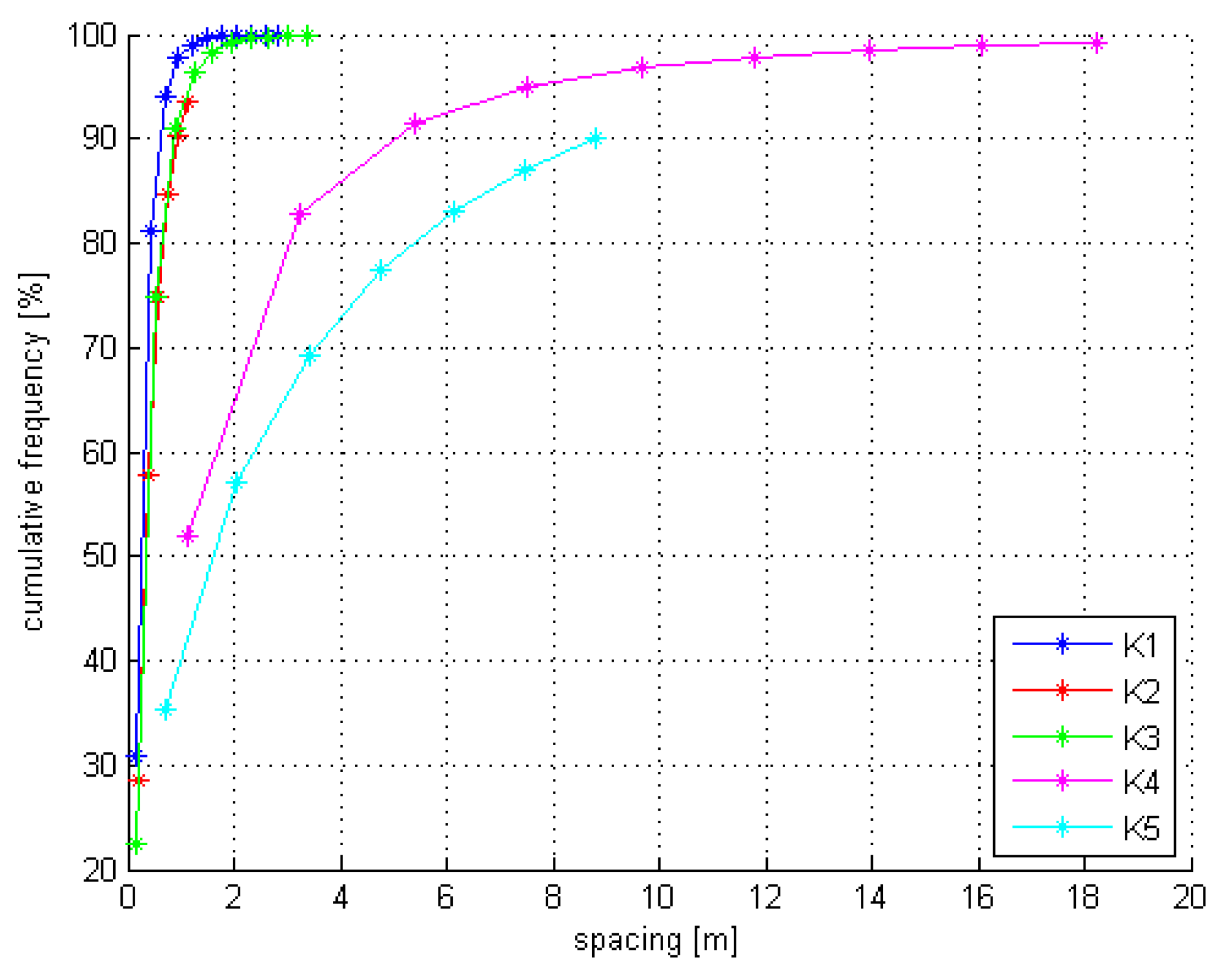
| Set | Dip | Dip Direction | Spacing Range (m) |
|---|---|---|---|
| K1 | 50 | 310 | 0.07–2.87 |
| K2 | 70 | 170 | - |
| K3a | 70 | 080 | 0.08–1.60 |
| K3b | 80 | 260 | |
| K4 | 60 | 030 | 0.30–19.21 |
| K5 | 40 | 240 | 2.72–9.43 |
| Set | Number of Data | Distribution | p-Value | Best Performance |
|---|---|---|---|---|
| K1 | 266 | Gamma | 0.061 | Log-normal |
| Log-normal | 0.148 | |||
| K2 | 12 | Gamma | 0.480 | Log-normal |
| exponential | 0.349 | |||
| Log-normal | 0.718 | |||
| Weibull | 0.488 | |||
| K3 | 241 | Log-normal | 0.263 | Log-normal |
| K4 | 121 | Weibull | 0.024 | Log-normal |
| Log-normal | 0.078 | |||
| K5 | 26 | Gamma | 0.166 | Gamma |
| exponential | 0.010 | |||
| Log-normal | 0.099 | |||
| Weibull | 0.128 |
| Set | SM [m] | DM [m] |
|---|---|---|
| K1 | 0.283 | 0.293 |
| K2 | 0.463 | 0.472 |
| K3 | 0.429 | 0.434 |
| K4 | 2.020 | 2.183 |
| K5 | 3.249 | 3.611 |
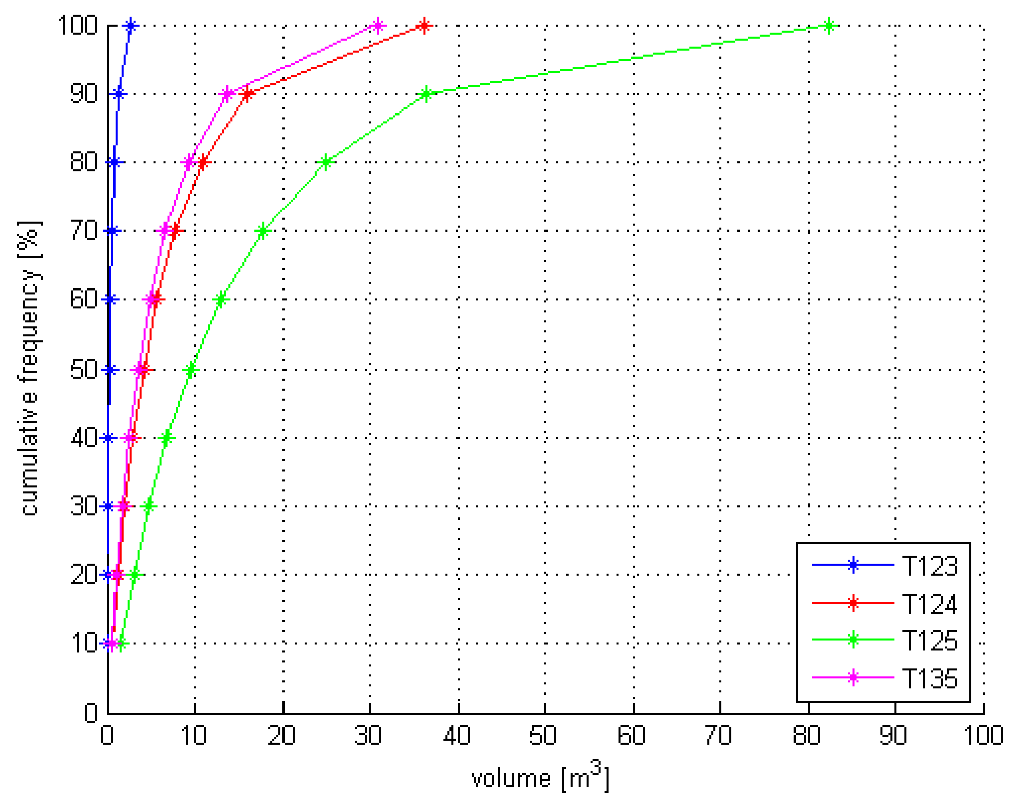
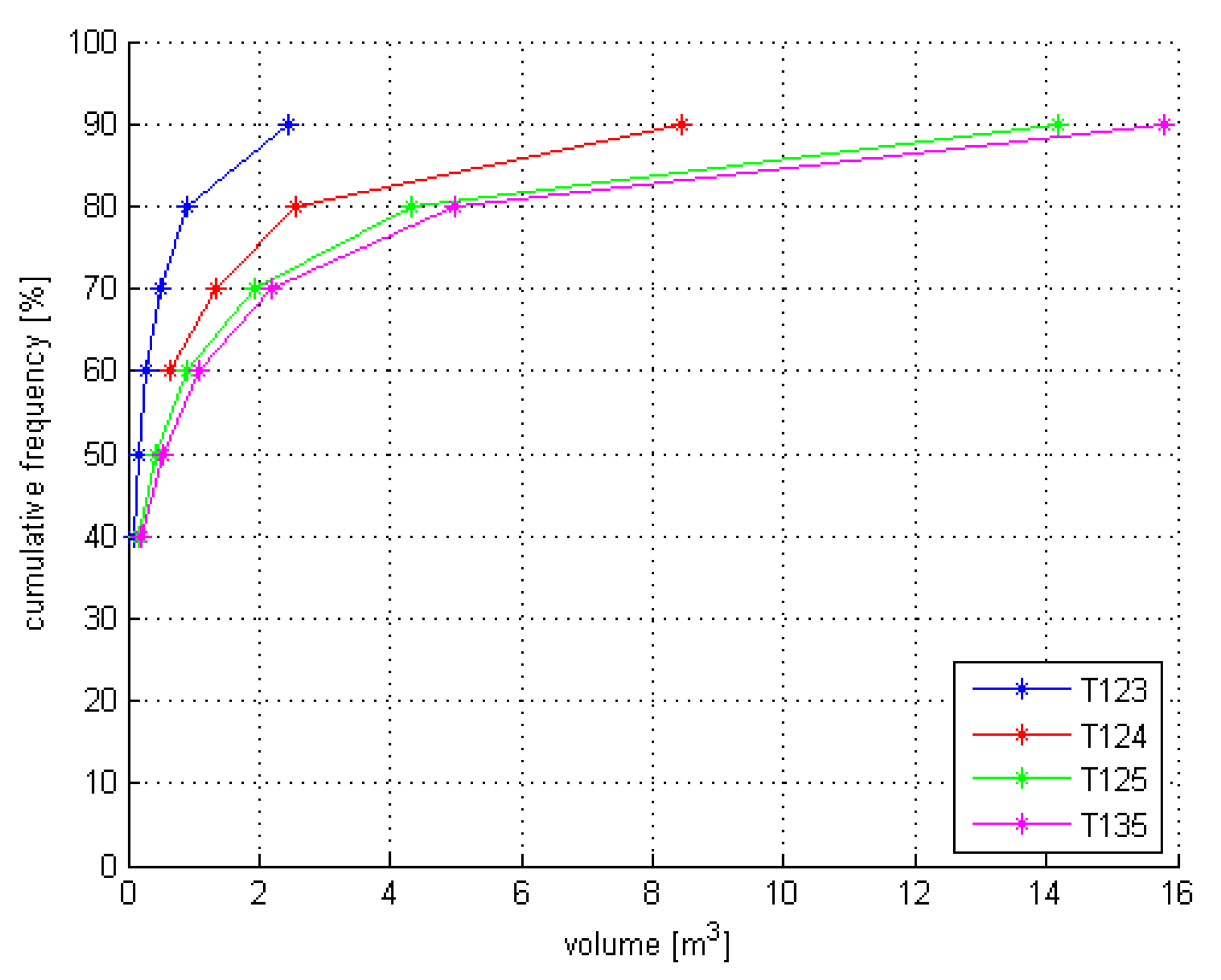
| Tern | Vsm [m3] | Ratio Vsm/VMCDF(50%) | Vdm [m3] | Ratio Vdm/VMCDF(50%) |
|---|---|---|---|---|
| T123 | 0.28 | 2.17 | 0.29 | 2.32 |
| T124 | 0.78 | 3.17 | 0.88 | 3.57 |
| T125 | 1.21 | 2.91 | 1.41 | 3.40 |
| T135 | 1.35 | 2.92 | 1.55 | 3.37 |
| Tern | Ratio VIBSD(100%)/SVmax [-] | Ratio VMCDF(95%)/SVmax [-] | ||
|---|---|---|---|---|
| Parallelepiped | Ellipsoid | Parallelepiped | Ellipsoid | |
| T123 | 17.7 | 11.2 | 33.5 | 21.1 |
| T124 | 243.3 | 153.4 | 134.4 | 84.7 |
| T125 | 549.5 | 346.4 | 223.4 | 140.8 |
| T135 | 204.5 | 128.9 | 242.9 | 153.1 |
© 2020 by the authors. Licensee MDPI, Basel, Switzerland. This article is an open access article distributed under the terms and conditions of the Creative Commons Attribution (CC BY) license (http://creativecommons.org/licenses/by/4.0/).
Share and Cite
Umili, G.; Bonetto, S.M.R.; Mosca, P.; Vagnon, F.; Ferrero, A.M. In Situ Block Size Distribution Aimed at the Choice of the Design Block for Rockfall Barriers Design: A Case Study along Gardesana Road. Geosciences 2020, 10, 223. https://doi.org/10.3390/geosciences10060223
Umili G, Bonetto SMR, Mosca P, Vagnon F, Ferrero AM. In Situ Block Size Distribution Aimed at the Choice of the Design Block for Rockfall Barriers Design: A Case Study along Gardesana Road. Geosciences. 2020; 10(6):223. https://doi.org/10.3390/geosciences10060223
Chicago/Turabian StyleUmili, Gessica, Sabrina Maria Rita Bonetto, Pietro Mosca, Federico Vagnon, and Anna Maria Ferrero. 2020. "In Situ Block Size Distribution Aimed at the Choice of the Design Block for Rockfall Barriers Design: A Case Study along Gardesana Road" Geosciences 10, no. 6: 223. https://doi.org/10.3390/geosciences10060223