Large-Scale Spatial Modeling of Crop Coefficient and Biomass Production in Agroecosystems in Southeast Brazil


Abstract
:
1. Introduction
2. Materials and Methods
2.1. Data Used
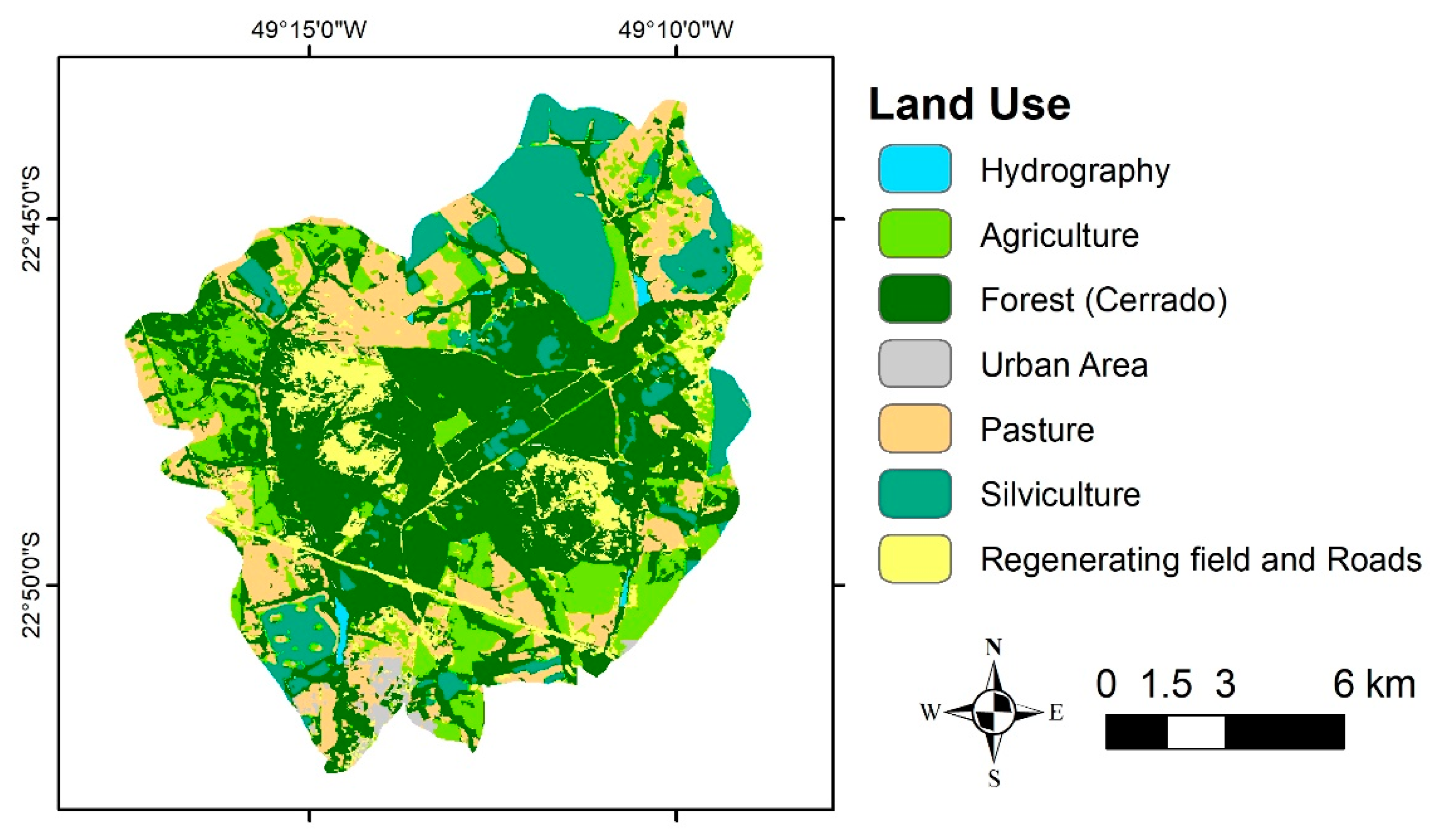
2.2. Study Area
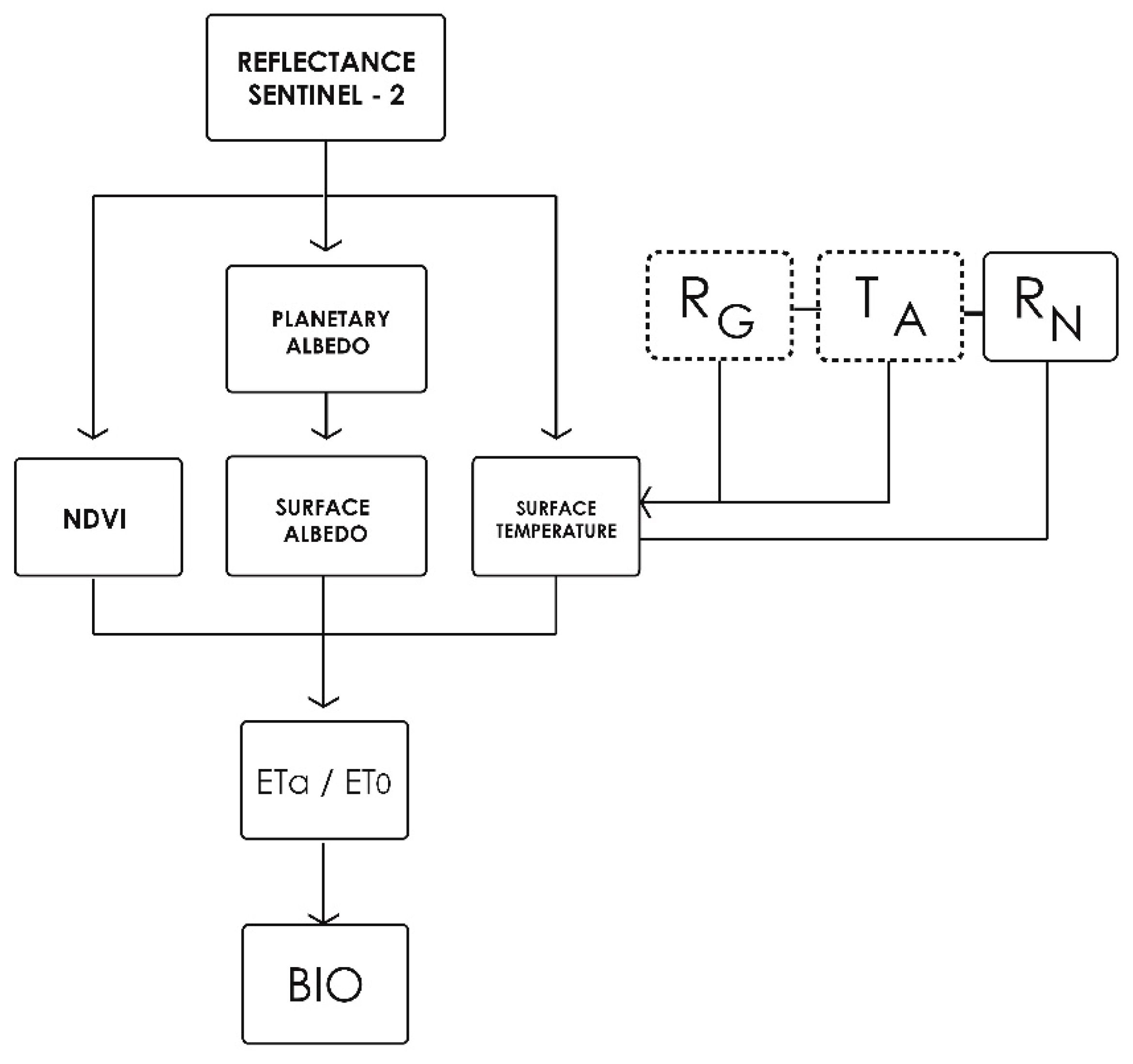
2.3. Simple Algorithm for Evapotranspiration Retrivieng (SAFER)
2.4. Monteith Model of Biomass Production
3. Results and Discussion
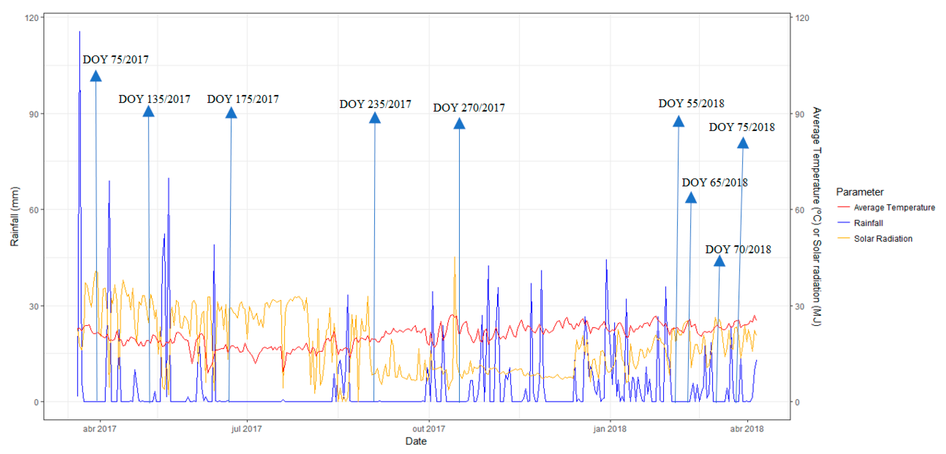
3.1. Weather Drivers
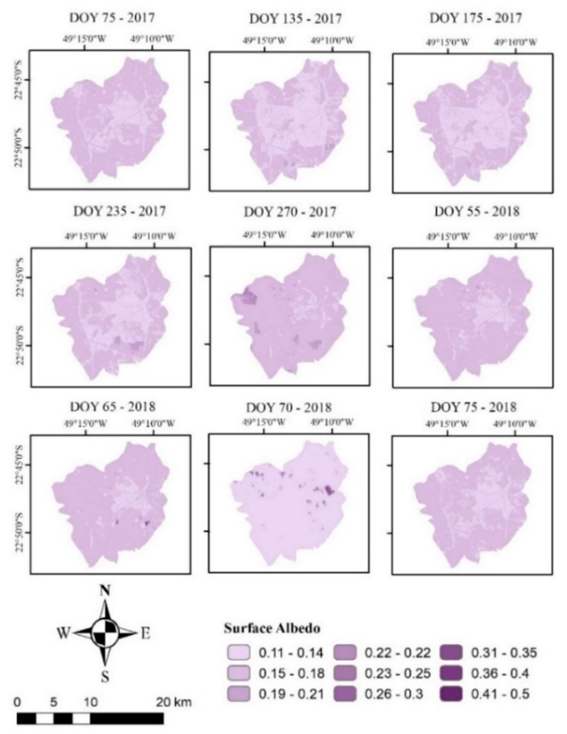
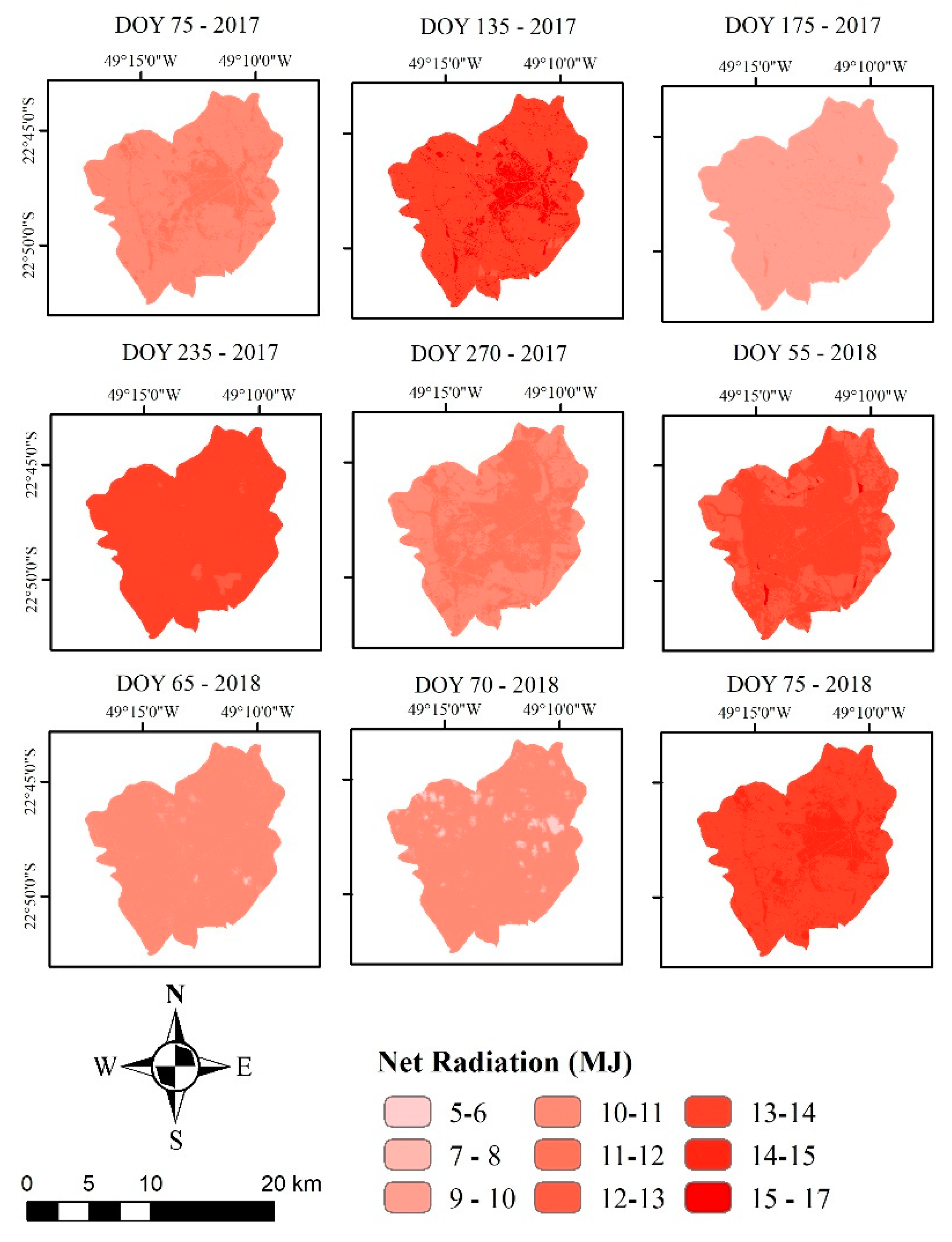
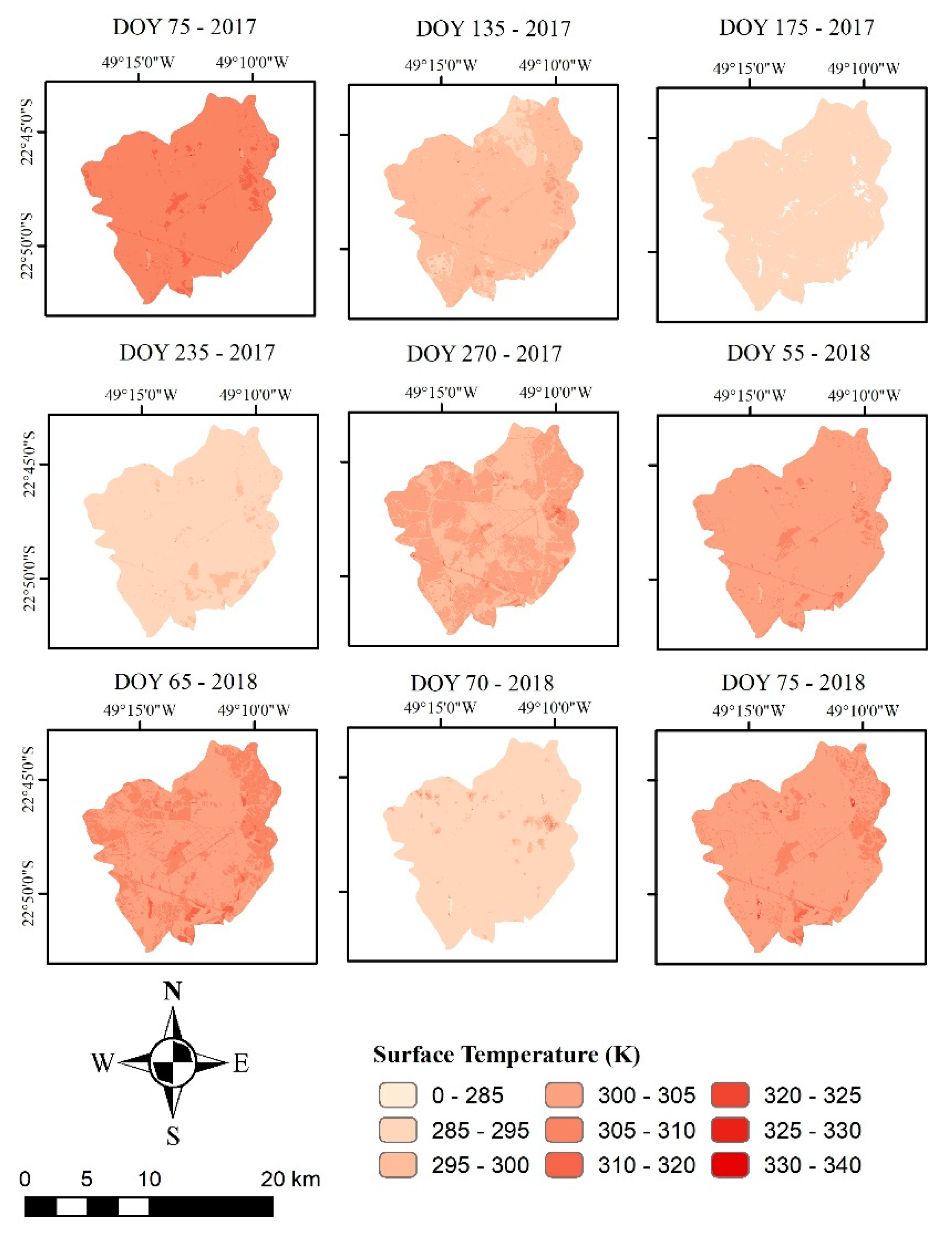
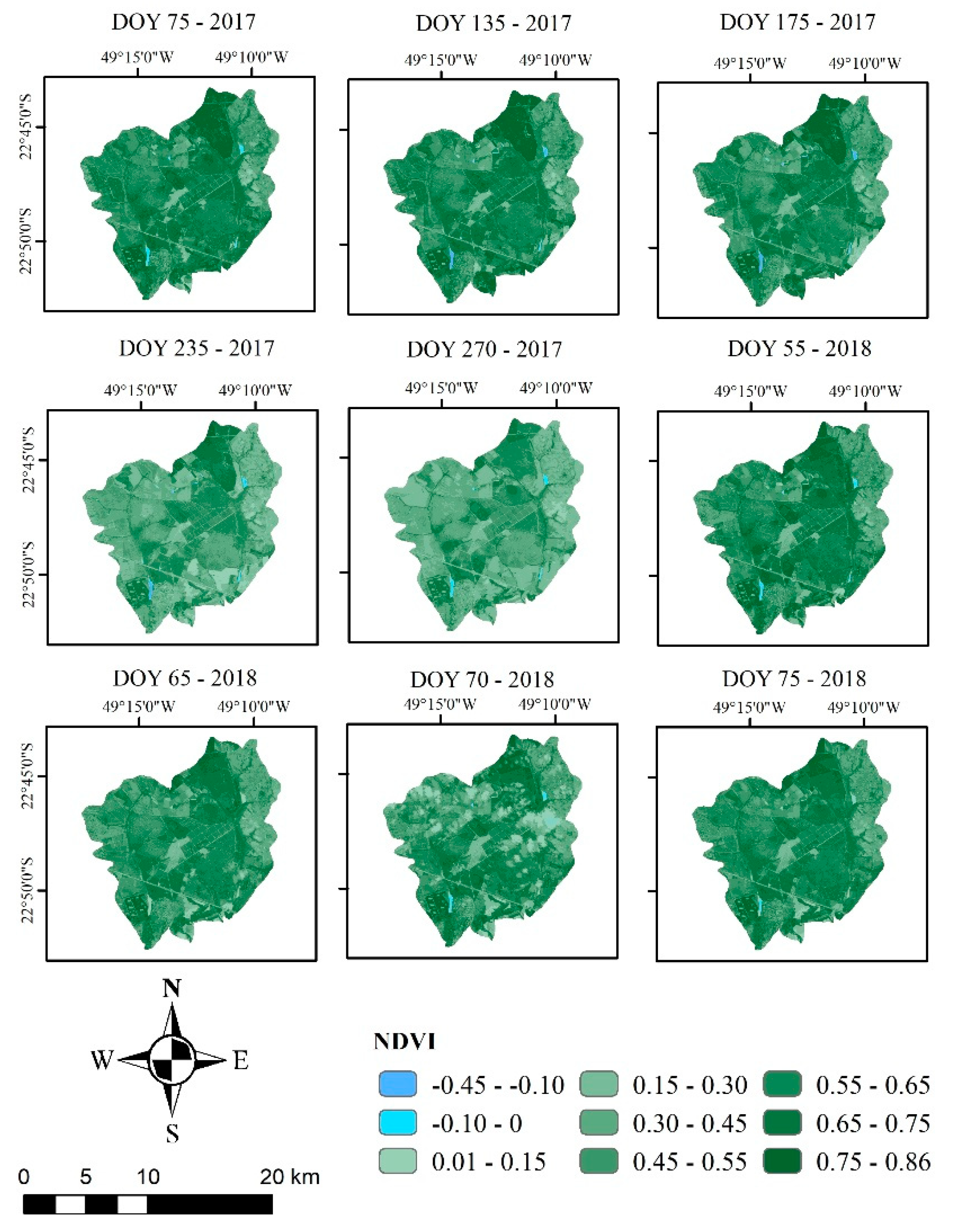
3.2. Input Parameters of SAFER Algorithm
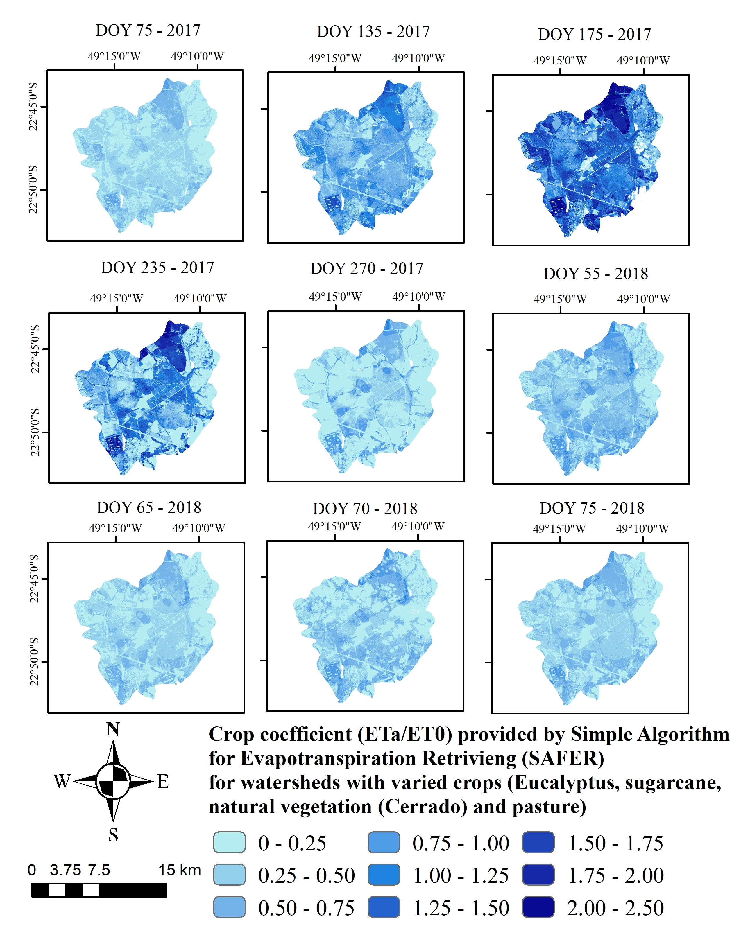
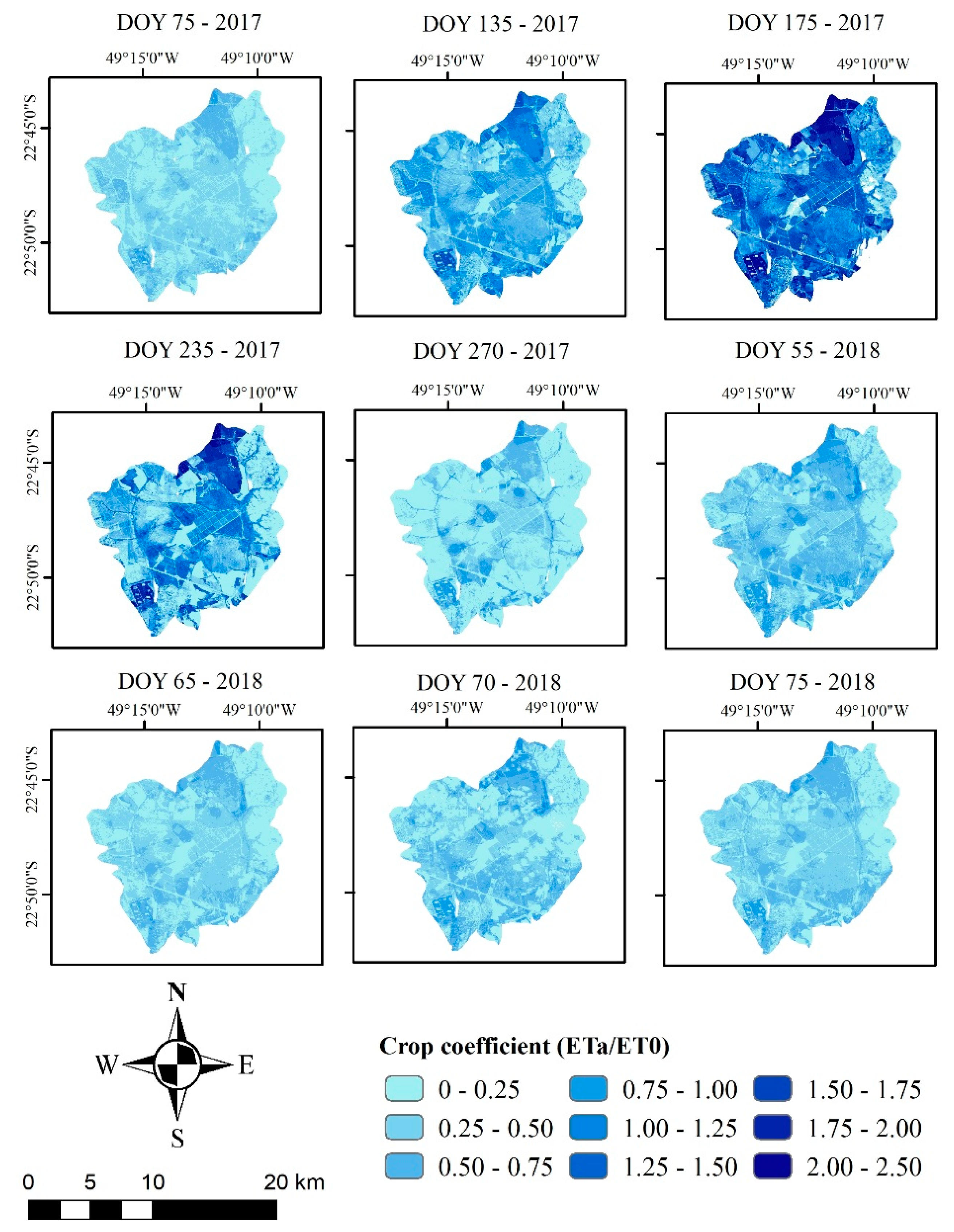
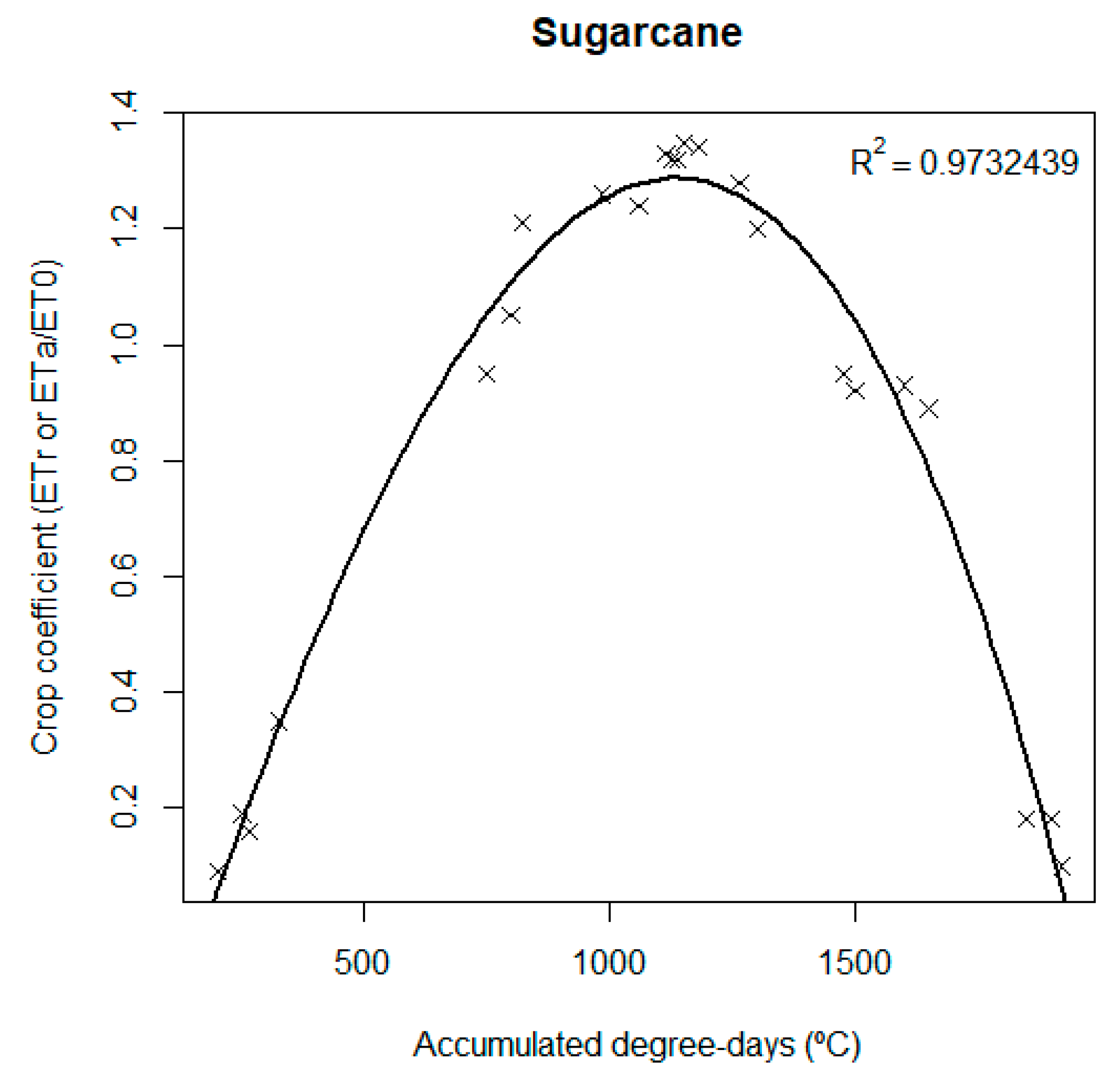
3.3. Crop Coefficient
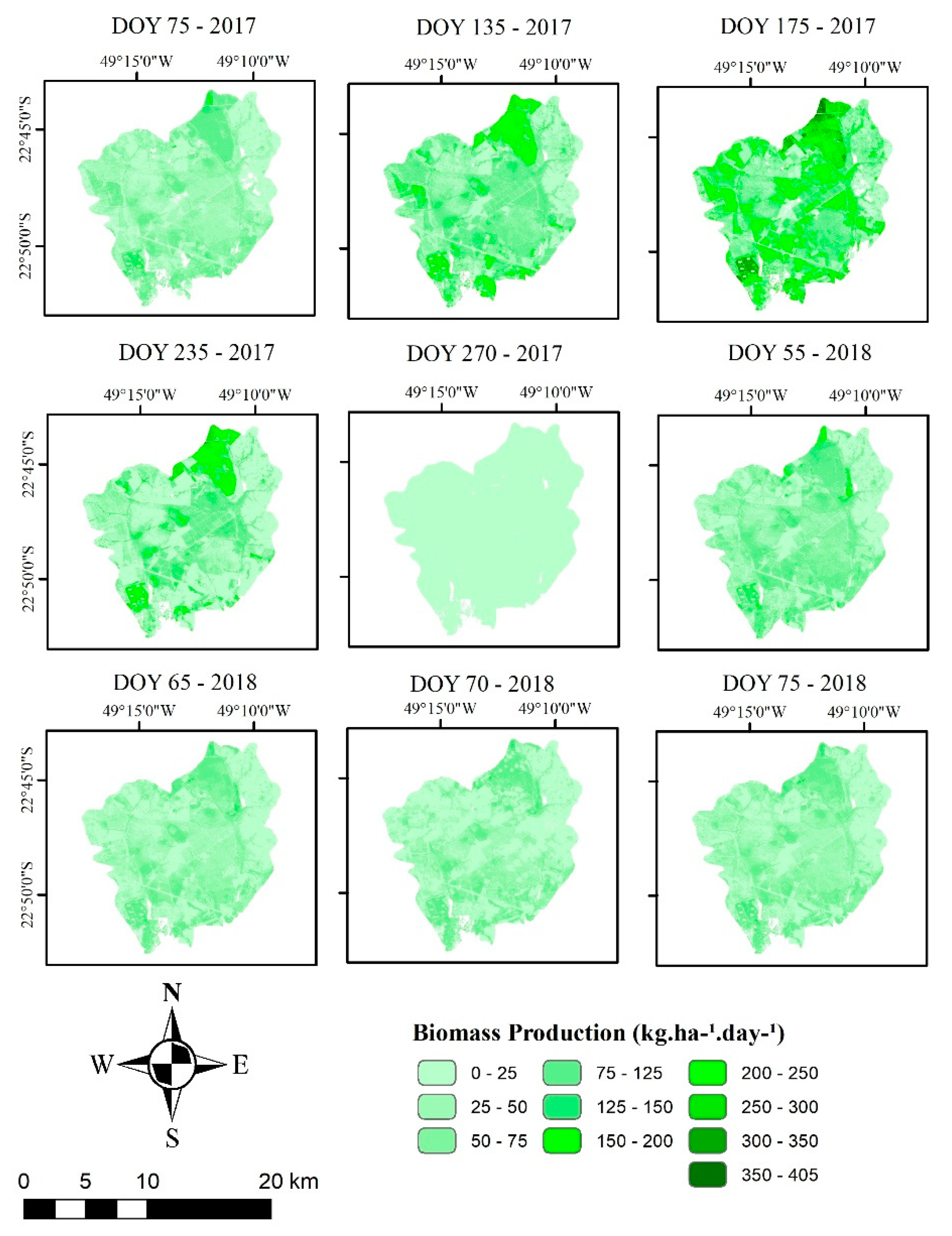
3.4. Biomass Production
4. Conclusions
Author Contributions
Funding
Acknowledgments
Conflicts of Interest
References
- Allen, R.G.; Pereira, L.S.; Raes, D.; Smith, M. Crop Evapotranspiration, Guidelines for Computing Crop Water Requirements; FAO Irrigation and Drainage Paper 56; FAO: Italy, Rome, 1998; 300p. [Google Scholar]
- ANA (Brazilian National Water Agency). Atlas Irrigation: Water Use in Irrigated Agriculture; Ministry of Environment: Brasília, Brazil, 2017; pp. 125–127. (In Portuguese)
- Kenny, J.F.; Barber, N.L.; Hutson, S.S.; Linsey, K.S.; Lovelace, J.K. Estimated Use of Water in the United States in 2005; U.S. Geology Survey Circular: Reston, VA, USA, 2009. [Google Scholar]
- Piccinni, G.; Ko, J.; Marek, T.; Howell, T. Determination of growth-stage-specific crop coefficients (Kc) of maize and sorghum. Agric. Water Manag. 2009, 96, 1698–1704. [Google Scholar] [CrossRef]
- Irmak, S.; Kabenge, I.; Rudnick, D.; Knezevic, S.; Woodward, D.; Moravek, M. Evapotranspiration crop coefficients for mixed riparian plant community and transpiration crop coefficients for common reed, cottonwood and peach-leaf willow in the Platte River basin, Nebraska-USA. J. Hydrol. 2013, 48, 177–190. [Google Scholar] [CrossRef]
- Teixeira, A.H.C.; Hernandez, F.B.T.; Andrade, R.G.; Leivas, J.F.; Bolfe, E.L. Energy balance with Landsat images in irrigated central pivots with corn crop in the São Paulo state, Brazil. Proc. SPIE 2014, 9239, 92390O. [Google Scholar] [CrossRef]
- Teixeira, A.H.C.; Hernandez, F.B.T.; Andrade, R.G.; Victoria, D.C.; Bolfe, E.L. Corn water variable assessments from earth observation data in the São Paulo state, southeast Brazil. J. Hydraul. Eng. 2015, 1, 1–11. [Google Scholar] [CrossRef]
- Irmak, S.; Odhiambo, L.O.; Specht, J.E.; Djaman, K. Hourly and daily single and basal evapotranspiration crop coefficients as a function of growing degreedays, days after emergence, leaf area index, fractional green canopy cover, and plant phenology for soybean. Trans. ASABE 2013, 56, 1785–1803. [Google Scholar]
- Teixeira, A.H.C.; Scherer-Warren, M.; Hernandez, F.B.T.; Andrade, R.G.; Leivas, J.F. Large-Scale Water Productivity Assessments with MODIS Images in a Changing Semi-Arid Environment: A Brazilian Case Study. Remote Sens. 2013, 5, 5783–5804. [Google Scholar] [CrossRef] [Green Version]
- Bastiaanssen, W.G.M.; Menenti, M.; Feddes, R.A.; Holtslag, A.M. A remote sensing surface energy balance algorithm for land (SEBAL). 1. Formulation. J. Hydrol. 1998, 212–213, 198–212. [Google Scholar] [CrossRef]
- Roerink, G.J.; Su, Z.; Menenti, M. S-SEBI: A simple remote sensing algorithm to estimate the surface energy balance. Phys. Chem. Earth 2000, 25, 147–157. [Google Scholar] [CrossRef]
- Su, Z. The Surface Energy Balance System (SEBS) for estimation of turbulent heat fluxes. Hydrol. Earth Syst. Sci. 2002, 6, 85–99. [Google Scholar] [CrossRef]
- Teixeira, A.H.C.; Bastiaanssen, W.G.M.; Ahmad, M.; Bos, M.G. Reviewing SEBAL input parameters for assessing evapotranspiration and water productivity for the Low-Middle São Francisco River basin, Brazil Part B: Application to the regional scale. Agric. For. Meteorol. 2009, 149, 477–490. [Google Scholar] [CrossRef]
- Hernandez, F.B.T.; Neale, C.M.U.; Teixeira, A.H.C.; Taghvaeian, S. Determining large scale actual evapotranspiration using agrometeorological and remote sensing data in the Northwest of Sao Paulo State, Brazil. Acta Hortic. 2014, 1038, 263–270. [Google Scholar] [CrossRef]
- Cutler, M.E.J.; Boyd, D.S.; Foody, G.M.; Vetrivel, A. Estimating tropical forest biomass with a combination of SAR image texture and Landsat TM data: An assessment of predictions between regions. ISPRS J. Photogramm. Remote Sens. 2012, 70, 66–77. [Google Scholar] [CrossRef] [Green Version]
- Silva, M.A.V.; Moscon, E.S.; Santana, C.C. Determination of biomass production of cotton using satellite images and spectral indexes. J. Hyperspectr. Remote Sens. 2017, 7, 73–81. [Google Scholar] [CrossRef]
- Rezende, A.V.; Vale, A.T.; Sanquetta, C.R.; Figueiredo Filho, A.; Felfili, J.M. Comparação de modelos matemáticos para estimativa do volume, biomassa e estoque de carbono da vegetação lenhosa de um cerrado sensu stricto em Brasília, DF. Scientia Forestalis 2006, 71, 65–76. (In Portuguese) [Google Scholar]
- Monteith, J.L. Solar radiation and productivity in tropical ecosystems. J. Appl. Ecol. 1972, 9, 747–766. [Google Scholar] [CrossRef]
- Daughtry, C.S.T.; Gallo, K.P.; Goward, S.N.; Prince, S.D.; Kustas, W.D. Spectral estimates of absorbed radiation and phytomass production in corn and soybean canopies. Remote Sens. Environ. 1992, 39, 141–152. [Google Scholar] [CrossRef]
- Gower, S.T.; Kucharik, C.J.; Norman, J.M. Direct and indirect estimation of leaf area index, fAPAR, and net primary production of terrestrial ecosystems. Remote Sens. Environ. 1999, 70, 29–51. [Google Scholar] [CrossRef]
- Daughtry, C.S.T.; Walthall, C.L.; Kim, M.S.; Colstoun, E.B.; Mcmurtrey, J.E., III. Estimating corn leaf clorofila concentration from leaf and canopy reflectance. Remote Sens. Environ. 2000, 74, 229–239. [Google Scholar] [CrossRef]
- Mandanici, E.; Bitelli, G. Preliminary Comparison of Sentinel-2 and Landsat 8 Imagery for a Combined Use. Remote Sens. 2016, 8, 1014. [Google Scholar] [CrossRef]
- Teixeira, A.H.C.; Leivas, J.F.; Andrade, R.G.; Hernandez, F.B.T. Water productivity assessments with Landsat 8 images in the Nilo Coelho irrigation scheme. Irriga 2015, 1, 1–10. [Google Scholar] [CrossRef]
- Teixeira, A.H.C.; Leivas, J.F.; Silva, G.B. Large-scale radiation and energy balances with Landsat 8 images and agrometeorological data in the Brazilian semiarid region. J. Appl. Remote Sens. 2017, 11, 016030. [Google Scholar] [CrossRef]
- Coaguila, D.N.; Hernandez, F.B.T.; Teixeira, A.H.C.; Franco, R.A.M.; Leivas, J.F. Water productivity using SAFER—Simple Algorithm for Evapotranspiration Retrivieng in watershed. Rev. Bras. Eng. Agríc. Ambient. 2017, 21, 524–529. [Google Scholar] [CrossRef]
- Teixeira, A.H.C.; Leivas, J.F.; Bayma-Silva, G. Options for using Landsat and RapidEye satellite images aiming the water productivity assessments in mixed agro-ecosystems. Proc. SPIE 2016, 9998, 99980A. [Google Scholar] [CrossRef]
- Teixeira, A.H.C.; Padovani, C.R.; Andrade, R.G.; Leivas, J.F.; Victoria, D.C.; Galdino, S. Use of MODIS images to quantify the radiation and energy balances in the Brazilian Pantanal. Remote Sens. 2015, 7, 14597–14619. [Google Scholar] [CrossRef]
- Vuolo, F.; Żółtak, M.; Pipitone, C.; Zappa, L.; Wenng, H.; Immitzer, M.; Weiss, M.; Baret, F.; Atzberger, C. Data Service Platform for Sentinel-2 Surface Reflectance and Value-Added Products: System Use and Examples. Remote Sens. 2016, 20, 938. [Google Scholar] [CrossRef]
- R Core Team. R: A Language and Environment for Statistical Computing. R Foundation for Statistical Computing. Available online: https://www.r-project.org/ (accessed on 7 August 2018).
- ESRI. GIS Mapping Software, Spatial Data Analytics & Location Platform. Environmental Systems Research Institute. Available online: http://www.esri.com/arcgis/ (accessed on 7 August 2018).
- Liu, W.T.H. Aplicações de Sensoriamento Remoto, 1st ed.; UNIDERP Publisher: Campo Grande, Brazil, 2007. (In Portuguese) [Google Scholar]
- CEPAGRI (Center for Meteorological and Climatic Research Applied to Agriculture). Climate of the Municipalities of São Paulo. Resource Document. Available online: http://www.cpa.unicamp.br/outras-informacoes/clima_muni_006.html (accessed on 7 January 2018). (In Portuguese).
- Silva, B.B.; Lopes, G.M.; Azevedo, P.V. Determinação do albedo de áreas irrigadas com base em imagens LANDSAT 5–TM. Rev. Bras. Meteorol. 2005, 13, 201–211. (In Portuguese) [Google Scholar]
- Teixeira, A.H.C.; Bastiaanssen, W.G.M.; Ahmad, M.D.; Bos, M.G. Analysis of energy fluxes and vegetation-atmosphere parametes in irrigated and natural ecosystems of semi-arid Brazil. J. Hydrol. 2008, 362, 110–127. [Google Scholar] [CrossRef]
- Teixeira, A.H.C.; Hernandez, F.B.T.; Lopes, H.L.; Scherer-Warren, M.; Bassoi, L.H. A comparative study of techniques for modeling the spatiotemporal distribution of heat and moisture fluxes in different agroecosystems in Brazil. In Remote Sensing of Energy Fluxes and Soil Moisture Content; Petropoulos, G.G., Ed.; CRC Group, Taylor and Francis: Boca Raton, FL, USA, 2014; pp. 169–191. [Google Scholar]
- Rouse, J.W.; Haas, R.H.; Deering, D.W.; Sehell, J.A. Monitoring the Vernal Advancement and Retrogradation (Green Wave Effect) of Natural Vegetation; Final Rep. RSC 1978-4; Remote Sensing Center, Texas A&M Univ.: College Station, TX, USA, 1974. [Google Scholar]
- Bruin, H.A.R.; Stricker, J.N.M. Evaporation of grass under non-restricted soil misture conditions. Hydrol. Sci. J. 2000, 45, 391–406. [Google Scholar] [CrossRef]
- Liou, Y.A.; Karm, S.K. Evapotranspiration estimating with remote sensing and various surface energy balance algorithms—A review. Energies 2014, 7, 2821–2849. [Google Scholar] [CrossRef]
- Teixeira, A.H.C. Determining Regional Actual Evapotranspiration of Irrigated Crops and Natural Vegetation in the Sâo Francisco River Basin (Brazil) Using Remote Sensing and Penman-Monteith Equation. Remote Sens. 2010, 2, 1287. [Google Scholar] [CrossRef] [Green Version]
- Doorenbos, J.; Kassan, A.H. Yield Response to Water; Irrigation and Drainage Paper, 33; FAO: Rome, Italy, 1979. [Google Scholar]
- Bastiaanssen, W.G.M.; Ali, S. A new crop yield forecasting model based on satellite measurements applied across the Indus basin, Pakistan. Agric. Ecosyst. Environ. 2003, 94, 321–340. [Google Scholar] [CrossRef]
- Queiroz, T.B.; Rocha, S.M.G.; Fonseca, F.S.A.; Alvarenga, I.C.A.; Martins, E.R. Efeitos do déficit hídrico no cultivo de mudas de Eucalipto. Irriga 2017, 22, 659. (In Portuguese) [Google Scholar] [CrossRef]
- Fernandes, J.L.; Ebecken, N.F.F.; Esquerdo, J.C.D.M. Sugarcane yield prediction in Brazil using NDVI time series and neural networks ensemble. Int. J. Remote Sens. 2017, 38, 4631–4644. [Google Scholar] [CrossRef]
- Bueno, M.R.; Teodoro, R.E.F.; Alvarenga, C.B.; Gonçalves, M.V. Determinação do coeficiente de cultura para o capim Tanzânia. Biosci. J. 2009, 25, 29–35. [Google Scholar]
- Manzione, R.L. Water table depths trends identification from cimatological anomalies ocurred between 2014 and 2016 in a cerrado conservation area in the Médio Paranapanema Hydrographic Region/SP-Brazil. Bol. Goiano de Geografia 2018, 38, 68–85. [Google Scholar] [CrossRef]
- André, R.G.B.; Mendonça, J.C.; Marques, V.S.; Pinheiro, F.M.A.; Marques, J. Aspectos energéticos do desenvolvimento da cana-de-açúcar. Parte 1: Balanço de radiação e parâmetros derivados. Rev. Bras. Meteorol. 2010, 25, 3, 375–382. [Google Scholar] [CrossRef]
- Giongo, P.R.; Vettorazzi, C.A. Albedo da superfície por meio de imagens TM-Landsat 5 e modelo numérico do terreno. Rev. Bras. Eng. Agríc. Ambient. 2014, 18, 833–838. (In Portuguese) [Google Scholar] [CrossRef] [Green Version]
- Giongo, P.R.; Moura, G.B.A.; Silva, B.B.; Rocha, H.R.; Medeiros, S.R.R.; Nazareno, A.C. Albedo à superfície a partir de imagens Landsat 5 em áreas de cana-de-açúcar e cerrado. Rev. Bras. Eng. Agríc. Ambient. 2010, 14, 279–287. [Google Scholar] [CrossRef] [Green Version]
- Cabral, O.M.R.; Rocha, H.R.; Ligo, M.A.V.; Brunini, O.; Dias, M.A.F.S. Fluxos turbulentos de calor sensível, vapor d’água e CO2 sobre plantação de cana-de-açúcar (Saccharum sp.) em Sertãozinho-SP. Rev. Bras. Meteorol. 2003, 18, 61–70. (In Portuguese) [Google Scholar]
- Boegh, E.; Soegaard, H.; Thomsem, A. Evaluating evapotranspiration rates and surface conditions using Landsat TM to estimate atmospheric resistance and surface resistance. Remote Sens. Environ. 2002, 79, 329–343. [Google Scholar] [CrossRef]
- Lobell, D.B.; Asner, G.P. Moisture effects on soil reflectance. Soil Sci. Soc. Am. J. 2002, 66, 722–727. [Google Scholar] [CrossRef]
- Van Dijk, A.I.J.M.; Bruijnzeel, L.A.; Schellekens, J. Micrometeorology and water use of mixed crops in upland West Java, Indonesia. Agric. For. Meteorol. 2004, 124, 31–49. [Google Scholar] [CrossRef]
- Li, S.G.; Eugster, W.; Asanuma, J.; Kotani, A.; Davaa, G.; Oyunbaatar, D.; Sugita, M. Energy partitioning and its biophysical controls above a grazing steppe in central Mongolia. Agric. For. Meteorol. 2006, 137, 89–106. [Google Scholar] [CrossRef]
- Menezes, S.J.M.C.; Sediyama, G.C.; Soares, V.P.; Gleriani, J.M.; Andrade, R.G. Estimativa dos componentes do balanço de energia e da evapotranspiração em plantios de eucalipto utilizando o algoritmo SEBAL e imagem Landsat 5–TM. Árvore 2011, 35, 649–657. [Google Scholar] [CrossRef]
- Gomes, H.B.; Silva, B.B.; Cavalcante, E.P.; Rocha, H.R. Balanço de radiação em diferentes biomas no estado de São Paulo mediante imagens Landsat 5. Geociências 2009, 28, 153–164. (In Portuguese) [Google Scholar]
- Pereira, R.M.; Casaroli, D.; Vellame, L.M.; Alves Junior, J.; Evangelista, A.W.P. Sugarcane leaf area estimate obtained from the corrected Normalized Difference Vegetation Index (NDVI). Pesq. Agropec. Trop. 2016, 46, 140–148. [Google Scholar] [CrossRef]
- Castanheira, L.B.; Landim, P.M.B.; Lourenço, R.W. Variabilidade do índice de vegetação por diferença normalizada (NDVI) em áreas de reflorestamento: Floresta Estadual ‘Edmundo Navarro de Andrade’ (FEENA)/Rio Claro (SP). Geociências. 2014, 33, 449–456. (In Portuguese) [Google Scholar]
- Lucas, A.A.; Schuler, C.A.B. Análise do NDVI/NOAA em cana-de-açúcar e Mata Atlântica no litoral norte de Pernambuco, Brasil. Rev. Bras. Eng. Agríc. Ambient. 2007, 11, 607–614. [Google Scholar] [CrossRef]
- Lu, N.; Chen, S.; Wilske, B.; Sun, G.; Chen, J. Evapotranspiration and soil water relationships in a range of disturbed and undisturbed ecosystems in the semi-arid Inner Mongolia, China. J. Plant Ecol. 2011, 4, 49–60. [Google Scholar] [CrossRef] [Green Version]
- Mata-González, R.; McLendon, T.; Martin, D.W. The inappropriate use of crop transpiration coefficients (Kc) to estimate evapotranspiration in arid ecosystems: A review. Arid Land Res. Manag. 2005, 19, 285–295. [Google Scholar] [CrossRef]
- Zhou, L.; Zhou, G. Measurement and modeling of evapotranspiration over a reed (Phragmites australis) marsh in Northeast China. J. Hydrol. 2009, 372, 41–47. [Google Scholar] [CrossRef]
- Muniz, R.A.; Sousa, E.F.; Mendonça, J.C.; Esteves, B.S.; Lousada, L.L. Balanço de energia e evapotranspiração do capim Mombaça sob sistema de pastejo rotacionado. Rev. Bras. Meteorol. 2014, 29, 47–54. [Google Scholar] [CrossRef] [Green Version]
- Lima, J.E.F.; Silva, C.L.; Oliveira, C.A.S. Comparação da evapotranspiração real simulada e observada em uma bacia hidrográfica em condições naturais de cerrado. Rev. Bras. Eng. Agríc. Ambient. 2001, 5, 33–41. [Google Scholar] [CrossRef] [Green Version]
- Santana, R.C.; Barros, N.F.; Leite, H.G.; Comerford, N.B.; Novais, R.F. Estimativa da biomassa em plantios de eucalipto no Brasil. Árvore 2008, 32, 697–706. (In Portuguese) [Google Scholar] [CrossRef]
- Oliver, F.C.; Singles, A. Water use efficiency of irrigated sugarcane as affected by variety and row spacing. Proc. S. Afr. Sugar Technol. Assoc. 2003, 77, 347–351. [Google Scholar]
- Andrade, R.G.; Sediyama, G.; Soares, V.P.; Gleriani, R.G.; Menezes, S.J.M.C. Estimativa da produtividade da cana-de-açúcar utilizando o SEBAL e imagens Landsat. Rev. Bras. Meteorol. 2004, 29, 433–442. (In Portuguese) [Google Scholar] [CrossRef]
- Donaldson, R.A.; Redshaw, K.A.; Rhodes, R.; van Anterpen, R. Season effects on productivity of some commercial South African sugarcane cultivars, I: Biomass and radiation use efficiency. Proc. S. Afr. Sugar Technol. Assoc. 2008, 81, 517–527. [Google Scholar]
- Silva, G.B.; Teixeira, A.H.C.; Victoria, D.C.; Nogueira, S.F.; Leivas, J.F.; Nunez, D.N.C.; Herlin, V.R. Energy balance model applied to pasture experimental areas in São Paulo State, Brazil. Proc. SPIE 2016, 9998, 99981C. [Google Scholar]
- Silva, C.O.F.; Manzione, R.L.; Teixeira, A.H.C. Modelagem espacial da evapotranspiração e produtividade hídrica na porção paulista do afloramento do aquífero Guarani entre 2013 e 2015. Holos Environ. 2018, 18, 126–140. [Google Scholar] [CrossRef]
- Gaur, N.; Mohanty, B.P.; Kefauver, S.C. Effect of observation scale on remote sensing based estimates of evapotranspiration in a semi-arid row cropped orchard environment. Precis. Agric. 2017, 18, 762–778. [Google Scholar] [CrossRef]
- Vincini, M.; Calegari, F.; Casa, R. Sensitivity of leaf chlorophyll empirical estimators obtained at Sentinel-2 spectral resolution for different canopy structures. Precis. Agric. 2016, 17, 313–331. [Google Scholar] [CrossRef]


| DOY | Sugarcane Crop | Pasture | Silviculture | Forest |
|---|---|---|---|---|
| 75/2017 | 0.18 ± 0.001 | 0.23 ± 0.001 | 0.17 ± 0.001 | 0.16 ± 0.001 |
| 135/2017 | 0.17 ± 0.01 | 0.22 ± 0.001 | 0.16 ± 0.001 | 0.15 ± 0.001 |
| 175/2017 | 0.17 ± 0.01 | 0.21 ± 0.001 | 0.17 ± 0.01 | 0.14 ± 0.001 |
| 235/2017 | 0.16 ± 0.001 | 0.19 ± 0.01 | 0.17 ± 0.001 | 0.16 ± 0.001 |
| 270/2017 | 0.17 ± 0.001 | 0.20 ± 0.001 | 0.18 ± 0.001 | 0.17 ± 0.01 |
| 55/2018 | 0.23 ± 0.01 | 0.20 ± 0.01 | 0.17 ± 0.01 | 0.16 ± 0.001 |
| 65/2018 | 0.20 ± 0.001 | 0.21 ± 0.001 | 0.18 ± 0.001 | 0.16 ± 0.001 |
| 70/2018 | 0.20 ± 0.001 | 0.21 ± 0.03 | 0.11 ± 0.06 | 0.12 ± 0.001 |
| 75/2018 | 0.21 ± 0.001 | 0.21 ± 0.001 | 0.14 ± 0.001 | 0.13 ± 0.001 |
| DOY | Sugarcane Crop | Pasture | Silviculture | Forest |
|---|---|---|---|---|
| 75/2017 | 12.61 ± 0.21 | 12.70 ± 0.23 | 12.79 ± 0.18 | 12.84 ± 0.19 |
| 135/2017 | 15.49 ± 0.29 | 15.62 ± 0.25 | 15.74 ± 0.21 | 15.86 ± 0.21 |
| 175/2017 | 9.53 ± 0.17 | 9.60 ± 0.18 | 9.70 ± 0.15 | 9.80 ± 0.15 |
| 235/2017 | 11.32 ± 0.24 | 11.45 ± 0.18 | 11.59 ± 0.15 | 11.65 ± 0.15 |
| 270/2017 | 10.66 ± 0.30 | 10.83 ± 0.19 | 11.02 ± 0.17 | 11.01 ± 0.26 |
| 55/2018 | 14.86 ± 0.24 | 14.97 ± 0.27 | 15.17 ± 0.23 | 15.24 ± 0.22 |
| 65/2018 | 9.21 ± 0.16 | 9.25 ± 0.21 | 9.38 ± 0.13 | 9.41 ± 0.18 |
| 70/2018 | 10.91 ± 0.85 | 10.94 ± 0.94 | 10.90 ± 1.29 | 11.02 ± 1.16 |
| 75/2018 | 13.67 ± 0.17 | 13.73 ± 0.22 | 13.88 ± 0.16 | 13.94 ± 0.17 |
| DOY | Sugarcane Crop | Pasture | Silviculture | Forest |
|---|---|---|---|---|
| 75/2017 | 307.87 ± 1.85 | 307.73 ± 1.18 | 306.63 ± 1.59 | 306.98 ± 1.43 |
| 135/2017 | 297.05 ± 1.95 | 296.98 ± 1.15 | 295.67 ± 1.53 | 295.05 ± 1.35 |
| 175/2017 | 289.23 ± 1.41 | 289.42 ± 0.93 | 287.95 ± 1.27 | 288.42 ± 1.01 |
| 235/2017 | 292.71 ± 2.25 | 291.80 ± 1.40 | 289.44 ± 1.99 | 290.01 ± 2.02 |
| 270/2017 | 302.50 ± 1.80 | 301.46 ±1.47 | 299.59 ± 2.04 | 299.91 ± 2.61 |
| 55/2018 | 302.88 ± 1.72 | 302.73 ± 1.35 | 301.75 ± 1.50 | 301.87 ± 1.39 |
| 65/2018 | 305.62 ± 1.97 | 305.32 ± 1.35 | 304.26 ± 1.48 | 304.50 ± 1.39 |
| 70/2018 | 304.23 ± 1.64 | 304.02 ± 1.25 | 303.27 ± 1.89 | 303.48 ± 1.95 |
| 75/2018 | 304.68 ± 1.97 | 304.30 ± 1.16 | 303.35 ± 1.38 | 303.55 ± 1.30 |
| DOY | Sugarcane Crop | Pasture | Silviculture | Forest |
|---|---|---|---|---|
| 75/2017 | 0.63 ± 0.05 | 0.33 ± 0.01 | 0.68 ± 0.05 | 0.63 ± 0.03 |
| 135/2017 | 0.56 ± 0.07 | 0.30 ± 0.01 | 0.69 ± 0.07 | 0.62 ± 0.03 |
| 175/2017 | 0.59 ± 0.07 | 0.28 ± 0.01 | 0.68 ± 0.07 | 0.60 ± 0.02 |
| 235/2017 | 0.54 ± 0.04 | 0.24 ± 0.09 | 0.58 ± 0.08 | 0.49 ± 0.03 |
| 270/2017 | 0.57 ± 0.01 | 0.23 ± 0.08 | 0.52 ± 0.06 | 0.48 ± 0.05 |
| 55/2018 | 0.55 ± 0.05 | 0.22 ± 0.01 | 0.65 ± 0.06 | 0.62 ± 0.03 |
| 65/2018 | 0.58 ± 0.06 | 0.28 ± 0.01 | 0.62 ± 0.05 | 0.58 ± 0.03 |
| 70/2018 | 0.56 ± 0.08 | 0.27 ± 0.02 | 0.58 ± 0.02 | 0.54 ± 0.09 |
| 75/2018 | 0.59 ± 0.06 | 0.32 ± 0.01 | 0.64 ± 0.05 | 0.61 ± 0.02 |
| DOY | Sugarcane Crop | Pasture | Silviculture | Forest |
|---|---|---|---|---|
| 75/2017 | 0.95 ± 0.18 | 0.59 ± 0.14 | 1.19 ± 0.21 | 1.05 ± 0.31 |
| 135/2017 | 1.21 ± 0.41 | 0.65 ± 0.25 | 1.30 ± 0.35 | 1.15 ± 0.25 |
| 175/2017 | 1.35 ± 0.43 | 0.94 ± 0.29 | 1.56 ± 0.39 | 1.25 ± 0.24 |
| 235/2017 | 1.24 ± 0.29 | 0.81 ± 0.26 | 1.45 ± 0.27 | 1.17 ± 0.25 |
| 270/2017 | 1.11 ± 0.21 | 0.61 ± 0.15 | 1.29 ± 0.32 | 1.16 ± 0.19 |
| 55/2018 | 0.95 ± 0.21 | 0.62 ± 0.21 | 1.26 ± 0.35 | 1.11 ± 0.21 |
| 65/2018 | 0.92 ± 0.22 | 0.56 ± 0.26 | 1.19 ± 0.29 | 1.05 ± 0.25 |
| 70/2018 | 0.93 ± 0.24 | 0.69 ± 0.32 | 1.19 ± 0.34 | 1.07 ± 0.26 |
| 75/2018 | 0.89 ± 0.29 | 0.68 ± 0.25 | 1.17 ± 0.35 | 1.12 ± 0.31 |
| DOY | Sugarcane Crop | Pasture | Silviculture | Forest |
|---|---|---|---|---|
| 75/2017 | 36.72 ± 29.34 | 26.78 ± 22.91 | 74.45 ± 42.10 | 46.10 ± 24.67 |
| 135/2017 | 69.91 ± 58.11 | 46.42 ± 35.27 | 139.88 ± 73.77 | 87.43 ± 42.47 |
| 175/2017 | 104.70 ± 74.30 | 73.10 ± 47.74 | 210.96 ± 98.53 | 134.04 ± 57.47 |
| 235/2017 | 22.28 ± 36.70 | 17.98 ± 22.25 | 137.42 ± 83.06 | 72.94 ± 46.89 |
| 270/2017 | 25.15 ± 1.25 | 15.63 ± 5.45 | 25.15 ± 7.25 | 30.45 ± 8.96 |
| 55/2018 | 45.28 ± 42.15 | 37.19 ± 29.14 | 79.68 ± 42.15 | 63.67 ± 34.94 |
| 65/2018 | 30.10 ± 31.36 | 24.83 ± 22.45 | 59.46 ± 36.80 | 43.50 ± 26.24 |
| 70/2018 | 26.40 ± 29.76 | 22.81 ± 23.23 | 51.28 ± 40.38 | 37.41 ± 28.80 |
| 75/2018 | 32.20 ± 29.15 | 27.96 ± 23.67 | 63.78 ± 38.25 | 46.53 ± 25.55 |
© 2018 by the authors. Licensee MDPI, Basel, Switzerland. This article is an open access article distributed under the terms and conditions of the Creative Commons Attribution (CC BY) license (http://creativecommons.org/licenses/by/4.0/).
Share and Cite
De Oliveira Ferreira Silva, C.; Lilla Manzione, R.; Albuquerque Filho, J.L. Large-Scale Spatial Modeling of Crop Coefficient and Biomass Production in Agroecosystems in Southeast Brazil. Horticulturae 2018, 4, 44. https://doi.org/10.3390/horticulturae4040044
De Oliveira Ferreira Silva C, Lilla Manzione R, Albuquerque Filho JL. Large-Scale Spatial Modeling of Crop Coefficient and Biomass Production in Agroecosystems in Southeast Brazil. Horticulturae. 2018; 4(4):44. https://doi.org/10.3390/horticulturae4040044
Chicago/Turabian StyleDe Oliveira Ferreira Silva, César, Rodrigo Lilla Manzione, and José Luiz Albuquerque Filho. 2018. "Large-Scale Spatial Modeling of Crop Coefficient and Biomass Production in Agroecosystems in Southeast Brazil" Horticulturae 4, no. 4: 44. https://doi.org/10.3390/horticulturae4040044