Anticipate Manning’s Coefficient in Meandering Compound Channels

Abstract

Estimating Manning’s roughness coefficient $(n)$ is one of the essential factors in predicting the discharge in a stream. Present research work is focused on prediction of Manning’s $n$ in meandering compound channels by using the Group Method of Data Handling Neural Network (GMDH-NN) approach. The width ratio $(\alpha )$, relative depth $(\beta )$, sinuosity $(s)$, Channel bed slope $(S_o)$, and meander belt width ratio $(\omega )$ are specified as input parameters for the development of the model. The performance of GMDH-NN is evaluated with two different machine learning techniques, namely the support vector regression (SVR) and multivariate adaptive regression spline (MARS) with various statistical measures. Results indicate that the proposed GMDH-NN model predicts the Manning’s $n$ satisfactorily as compared to the MARS and SVR model. This GMDH-NN approach can be useful for practical implementation as the prediction of Manning’s coefficient and subsequently discharge through Manning’s equation in the compound meandering channels are found to be quite adequate.

1. Introduction

In river engineering, the Manning’s coefficient $(n)$ plays a vital role in the computation of flood discharge, velocity distribution, designing structures, calculating energy losses [1,2], and other hydraulic parameters. Accurate estimation of Manning’s roughness $(n)$ plays an important factor in flood conveyance estimation. Manning’s $n$ not only represented bed roughness, but also signifies the resistance to flow. Various equations are used for getting the discharge in simple channels using Manning’s $n$, Chezy’s $C$ and Darcy-Weisbach’s $f$ [3], but those equations are not adequate well, while predicting discharge in meandering compound channels. This study is focused on developing a machine learning based data-driven models for predicting Manning’s $n$. There are various elements that affect the resistance coefficient, such as the bed roughness, slope of the bed, geometry of the channel, and other parameters of a river.

Generally, the Manning’s formula is used for calculating the discharge in open channel flow. A significant amount of research has been carried out for selecting roughness coefficients for discharge calculation in an open channel. Cowan [4] considered the irregularity of the surface geometry of the channel, obstructions, and sinuosity to propose a model for predicting Manning’s roughness coefficient in meandering channels. The Soil Conservation Service (SCS) had developed an equation for estimating Manning’s $n$ for meandering channels by considering the sinuosity of the channel [5]. Limerinos [6] established a method for estimating the roughness coefficient by considering the various hydraulic parameters. Formulation for Manning’s roughness showing the gradient effect in channels having longitudinal slopes greater than 0.002 was derived by Jarrett [7]. Due to variation in flow depth, geometry and slope, the distinction of roughness coefficient in a straight channel as compared to a meandering channel were discussed by Arcement and Schneider [8]. Yen [9] proposed Manning’s $n$ for simple uniform flows taking account for a geometric measure, such as unevenness of the edge. Further, SCS method was linearized by James [10] for a meandering channel, named the Linearized SCS (LSCS) and recommended the Manning’s roughness value for the different sinuosity channels. Shiono et al. [11] developed a model to predict discharge considering the Manning’s n in the case of longitudinal slope and the meander effect of the channel. Jena [12] proposed an equation to calculate the $n$ by considering the effect of channel width, longitudinal channel slope, and the flow depth of the channel. The variations of wetted area, wetted perimeter, and the velocity data on Manning’s roughness coefficient by considering the flow simulation and sediment transport in irrigated channels was investigated by Mailapalli et al. [13]. Khatua et al. [14,15,16] formulated a mathematical equation for roughness coefficients by varying the sinuosity and geometry of the meandering compound channel. Xia et al. [17] and Barati [18,19,20] carried out the experiments for predicting discharge by taking care of the effect of bed roughness. Dash et al. [21] modeled the Manning’s roughness coefficient by considering the aspect ratio, viscosity, slope of the bed, and sinuosity. Pradhan et al. [22] proposed an empirical formulation of predicting Manning’s $n$ by dimensional analysis for the compound meandering channel, which affects relative depth, width ratio, longitudinal channel slope, and sinuosity.

In the recent years, ML techniques have been successfully implemented for predicting complex phenomena in hydrology and hydraulics. Zhang et al. [23] used the concept of diversity in the Group Method of Data Handling (GMDH) method for the prediction of time series to improve the noise-immunity capability. Mrugalski [24] proposed a method for error estimation based on the dynamic GMDH and multiple inputs, as well as output neurons. Najafzadeh and Lim [25] optimized the neuro-fuzzy GMDH model by the particle swarm optimization process to forecast the localized scour.

Vapnik and Lerner [26] extended the generalized statistical learning theory and introduced a term $\epsilon$ representing the intensive loss function for measuring the risk intensity in the support vector machine algorithm (SVM). More details on SVM can be found from many publications [27,28,29,30]. Dibike et al. [31] appraised SVM for rainfall-runoff modeling and revealed the significance of SVM in the field of civil engineering. Pal and Goel [32] also used the SVM technique to determine the discharge and end-depth ratio for circular and semi-circular channels. Further, Han et al. [33] applied SVM methodology for flood forecasting. Genc et al. [34] used Machine learning (ML) algorithms, i.e., SVM, ANN, and k-nearest neighbor (k-NN) to predict the velocity in small streams. Samui et al. [35] compared that the multivariate adaptive regression splines (MARS) methodology with ANN and FEM model and perceived that the MARS gives best outcomes for the uplift capacity of the suction caisson. Samui and Kurup [36] used MARS and LSSVM for the prediction of the consolidation ratio of clay deposits. Samui [37] predicted the elastic modulus of rock using MARS and show the performances of the MARS model better than the ANN.

However, collecting the velocity, discharge data during high flows in rivers, especially during unsteady, non-uniform and high flows are very dangerous and difficult task. Under these circumstances, the Machine learning (ML) models are highly helpful as the alternative approach for predicting Manning’s $n$ and the discharge in hydraulics engineering.

2. Experimental Setup

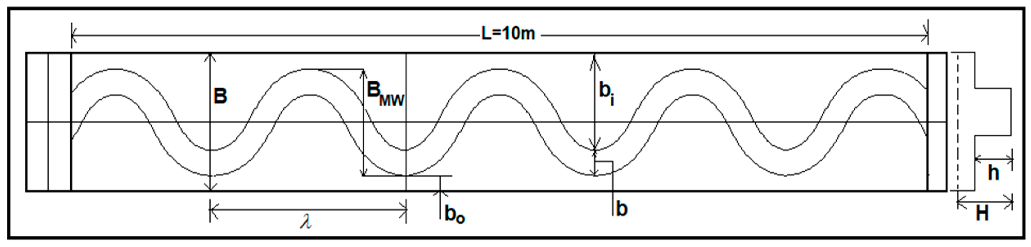
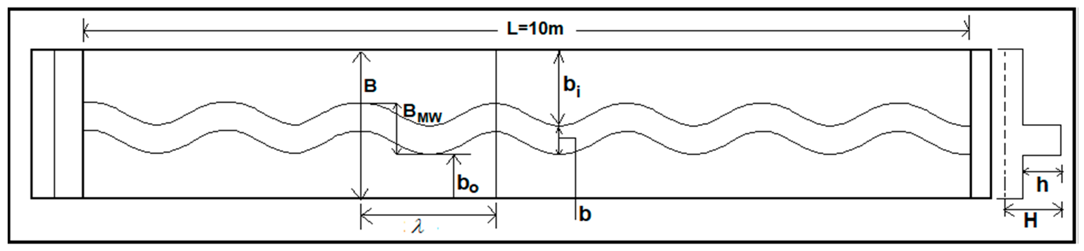
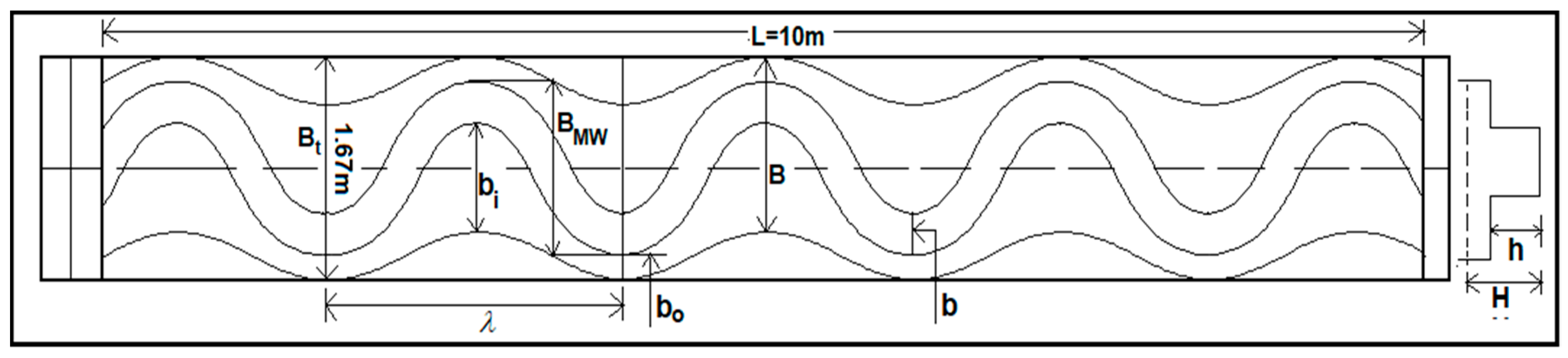
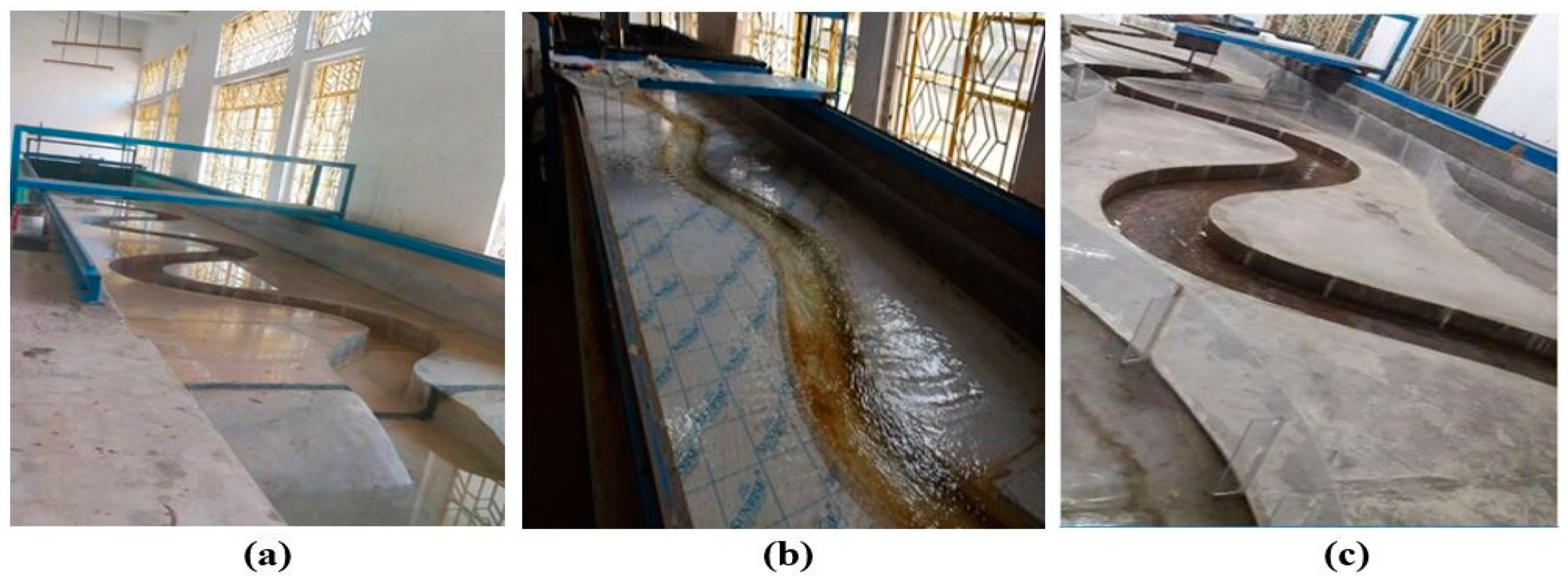
Experimental investigations are carried out in meandering compound channels with different sinuosity at the hydraulics-engineering laboratory under the department of civil engineering, National Institute of Technology Rourkela (NITR), India. The meandering compound channels are cast out of perspex sheets inside the flume of 10 m long, 1.7 m wide, and 0.25 m deep. The channel surfaces consist of the roughness coefficient as 0.01. Three types of experimental channels are set up for the present research works, as shown in Figure 1, Figure 2 and Figure 3. In the first and second type of meandering compound channels (NITR Type-I and NITR Type-II), the main channel is meandering with sinuosity 1.37 and 1.035, respectively, and is flanked by straight floodplain on both sides. The third one (NITR Type-III) is a doubly meandering compound channel, where both the main channel and floodplain levee are meandering with different sinuosity. Details of the experimental setup of these compound channels shown in

Table 1. Description of Geometric Parameters of the three Experimental Channel setup.

Sl. No	Channel Parameters	NITR Type-I *	NITR Type-II **	NITR Type-III ***
1	Types of channel	Meandering Compound Channel with straight floodplain	Meandering Compound Channel with straight floodplain	Doubly meandering compound channel
2	Type of Bed surface	Smooth	Smooth	Smooth
3	$\mathrm{Bed}\mathrm{Slope}\mathrm{of}\mathrm{the}\mathrm{Channel}(S_b)$	0.001	0.001	0.001
4	Angle $\mathrm{of}\mathrm{Arc}\mathrm{of}\mathrm{main}\mathrm{channel}({\varphi }_m)$	${60}^{\circ }$	${30}^{\circ }$	${60}^{\circ }$
5	Angle $\mathrm{of}\mathrm{Arc}\mathrm{of}\mathrm{floodplain}({\varphi }_f)$	0	0	${30}^{\circ }$
6	$\mathrm{Sin}\mathrm{uosity}\mathrm{of}\mathrm{the}\mathrm{main}\mathrm{channel}(s_m)$	1.37	1.035	1.37
7	$\mathrm{Sin}\mathrm{uosity}\mathrm{of}\mathrm{the}\mathrm{Floodplain}(s_f)$	1	1	1.035
8	Wavelength $\mathrm{of}\mathrm{the}\mathrm{channel}(\lambda )$	2.23 m	2.16 m	2.23 m
9	$\mathrm{Width}\mathrm{of}\mathrm{the}\mathrm{main}\mathrm{Channel}(b)$	0.28 m	0.28 m	0.28 m
10	Total $\mathrm{width}\mathrm{of}\mathrm{the}\mathrm{channel}(B)$	1.67 m	1.67 m	1.35 m
11	$\mathrm{Bank}\mathrm{Full}\mathrm{Depth}\mathrm{of}\mathrm{main}\mathrm{channel}(h)$	0.12 m	0.12 m	0.12 m
12	$\mathrm{Width}\mathrm{of}\mathrm{outer}\mathrm{Floodplain}(b_{\mathrm{o}})$	0.25 m	0.52 m	0.25 m
13	$\mathrm{Width}\mathrm{of}\mathrm{inner}\mathrm{floodplain}(b_f)$	1.14 m	0.87 m	0.82 m
14	$\mathrm{Meander}\mathrm{Belt}\mathrm{Width}(B_{MW})$	1.17 m	0.61 m	1.17 m

* Meandering compound channel of ${60}^{\circ }$ sinuosity with straight floodplain wall; ** Meandering compound channel of ${30}^{\circ }$ sinuosity with straight floodplain wall; *** Doubly meandering compound channel.

.

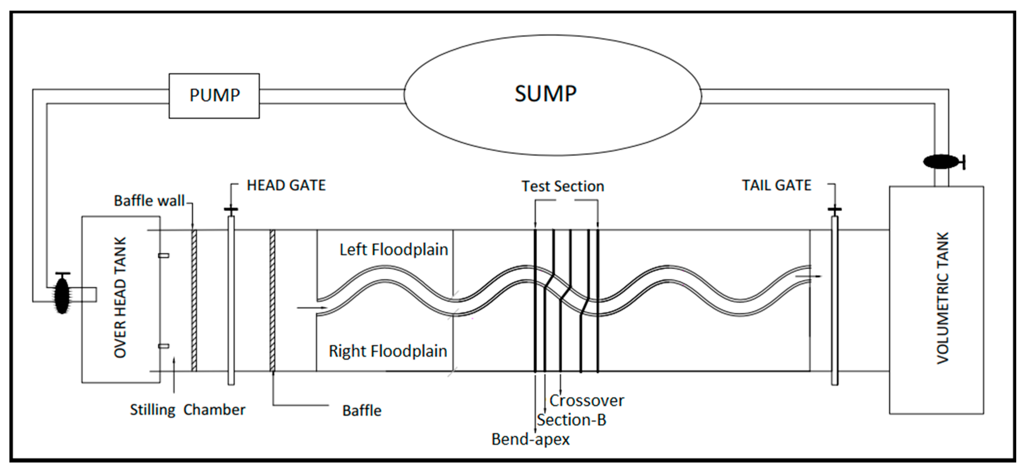
The bed slope of the channel is recorded as 0.001 for all the three types of channel. A movable bridge is placed across the flume with the facility of traversing on both the directions over the flume for taking measurements at different locations in the channel section. A measuring tank is situated at the downstream end of the flume. Water from the measuring tank is collected in a sump, which again feedbacks to the overhead tank with the help of a centrifugal pump. A closure valve is fitted at the downstream volumetric tank. A schematic illustration of the experimental setup of the compound meandering channel is shown in Figure 4. For a better understanding of the experimental channel setup, the sample photograph of NITR Type I, Type II, and Type III meandering compound channels are shown in Figure 5.

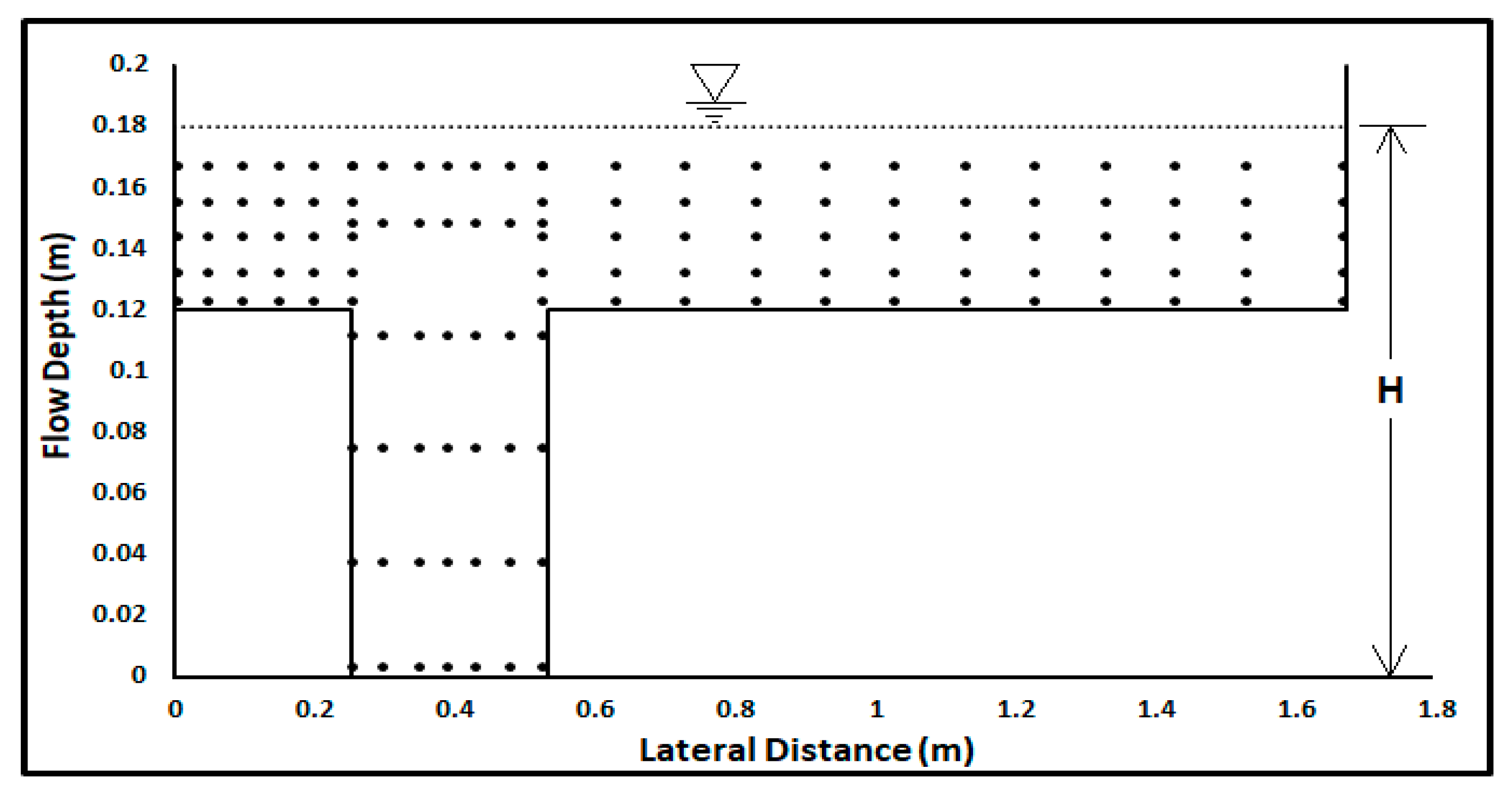
The measuring equipment involves point gauge having least count of 0.1 mm for measuring the flow depth in the channels. A Pitot tube coupled with manometer is used for measurement of pressure difference from which the point velocities of flow in the compound channels are computed. All of the readings are taken at the predefined grid points, as shown in Figure 6, at the bend apex, Section B and a geometric crossover of the three types of channels (Figure 4).

The Manning’s $n$ for the perspex sheet channel boundary is experimentally determined as 0.01. For this, the in-bank flow in the meandering main channel is collected in the volumetric tank located at its end. From the time-rise data of the water level in the volumetric tank, the discharge rate is computed. By knowing the channel cross-sectional area and the wetted perimeter, Manning’s $n$ is computed for four consecutive depths of flow, and the mean value of $n$ is computed as 0.01 [(0.0088 + 0.0096 + 0.0104 + 0.012)/4], which is found to be close to its value given various handbooks for the type of bed materials.

Traditional flow formulae are used for the estimation of discharge are Manning’s equation. From the observed discharge results, we can calculate Manning’s coefficient $n$ by the back calculation. After getting discharge, mean velocity $(V)$ can be computed by dividing area to the discharge. Then, from Manning’s equation, corresponding $n$ can be evaluated, which is given in the below equation:

$$n=\frac{{\mathrm{R}}^{\frac{2}{3}}{S}_o{}^{\frac{1}{2}}}{V}$$

(1)

where $V$ is indicated the mean velocity for the compound section of the compound channel, $S_o$ the bed slope of the compound channel, and $\mathrm{R}$ the hydraulic radius of the compound channel. It is known that Manning’s $n$ increases slightly with the depth of flow in the channel representing a lumped response to all of the flow resistances. Since the basic purpose of the present work is to model the Manning’s $n$ for overbank flow, the variation of observed $n$ value for the compound channel is shown in figure later in the manuscript.

Besides the present work, reported data of other researchers are also used to calibrate models for predicting Manning’s $n$ value. Other experimental works from which data is used in the present work are the FCF-B; the investigational studies done in the UK, Flood Channel Facility (FCF) during 1990–1992 on large-gauge meandering channels (Phase B). The data are acquired from the Birmingham university website (http://www.birmingham.ac.uk/) and also collected from other articles [10,38,39]. Other than FCF-B, the authors have also used data from Toebes-Sooky [40], Kar [41], Das [42], Kiely [43], Patra-Kar [44], Khatua [45], Mohanty [46], and Pradhan [22] to predict the roughness coefficient, as given in

Table 2. Hydraulics Parameter of the Experimental and Collected Dataset used in Present work.

Data Source	$\mathbf{Bed}\mathbf{Slope},{\mathit{S}}_{\mathit{o}}$	Top Width, $\mathit{B}$ (m)	Main Channel Depth, $\mathit{H}$ (m)	$\mathbf{Meander}\mathbf{Belt}\mathbf{Width},{\mathit{B}}_{\mathit{M}\mathit{W}(\mathbf{m})}$	$\mathit{\alpha }=\frac{\mathit{B}}{\mathit{b}}$	$\mathit{\beta }=\frac{(\mathit{H}-\mathit{h})}{\mathit{H}}$	$\mathbf{Sinuosity}(\mathit{s})$	$\mathbf{Discharge}{\mathit{Q}}_{\mathit{obs}}$ (m3/s)	Manning’s $\mathit{n}$
Toebes-Sooky (1967)	0–0.004	1.185	0.058–0.114	0.390	5.657	0.070–0.530	1.09	0.004–0.014	0.014–0.0165
Kar (1977)	0.002	0.525	0.116–0.170	0.904	5.250	0.138–0.410	1.220	0.004–0.0195	0.0158–0.0323
Das (1984)	0.004	0.213	0.122–0.154	1.000	2.130	0.180–0.349	1.210	0.0055–0.0128	0.0126–0.0171
Kiely (1989)	0.001	1.200	0.0547–0.09	0.642	6.000	0.086–0.441	1.22	0.0024–0.0163	0.0106–0.0146
FCF B (1990–1991)	0.001	6.107, 8.56, 10	0.153–0.303	0.611, 0.856, 1	6.79, 8.33, 11.11	0.017–0.505	1.374, 2.043	0.036–1.090	0.0098–0.029
Patra-Kar (2000)	0.003	1.380	0.295–0.316	1.380	3.136	0.153–0.210	1.043	0.095–0.110	0.0189–0.021
Khatua (2007)	0.003, 0.005	0.577, 1.930	0.097–0.184	0.443, 1.650	4.81, 16.08	0.123–0.339	1.44, 1.91	0.010–0.485	0.0105–0.0128
Mohanty (2013)	0.001	3.950	0.081–0.110	1.411	11.970	0.194–0.410	1.11	0.017–0.081	0.010–0.0135
Pradhan (2017)	0.002	3.950	0.085–0.10	0.924	11.970	0.235–0.350	4.11	0.028–0.052	0.0133–0.0150
NITR Type-I	0.001	1.670	0.140–0.195	1.170	5.964	0.137–0.385	1.37	0.035–0.063	0.0087–0.0125
NITR Type-II	0.001	1.670	0.14–0.194	0.610	6.036	0.143–0.381	1.035	0.023–0.059	0.0105–0.0126
NITR Type-III	0.001	1.350	0.138–0.195	1.170	4.821	0.130–0.385	1.37	0.019–0.050	0.0127–0.0214

. All of the experimental channel data used in the present work consists of similar hydraulic nature having smooth meandering compound channels.

Factors Affecting Roughness Coefficient

Studies [8,11,15,16,21,22,47,48] have indicated that Manning’s $n$ not only represent the resistance to the flow in the channel, but it represents the lumped response of all the hydraulic and geometric parameters influencing the flow in the channel. Therefore, in the current study, the author considers the influencing non-dimensional factors, such as the width ratio of the channel $(\alpha =B/b)$, depth ratio or relative depth $(\beta =(H-h)/H)$, sinuosity $(s)$, longitudinal channel slope $(S_o)$, and meander belt width ratio $(\omega =B_{MW}/B)$ as the inputs to model for predicting the Manning’s $n$ value. A regular channel retains diversity in flow and surface conditions that need to be incorporated to develop a suitable model for predicting the roughness coefficient at various flood conditions. It is important to incorporate all of these variables to predict a suitable roughness coefficient at all flood conditions.

For the present work, the Group Method of Data Handling neural network (GMDH-NN) algorithm is used to predict the roughness coefficient, which is compared with machine learning methods, such as the multivariate adaptive regression spline (MARS) and the support vector machine regression (SVR) models, for developing a best alternative for modelling Manning’s $n$ value for compound channels.

3. Theoretical Background

3.1. Group Method of Data Handling Neural Network (GMDH-NN)

GMDH-NN is a machine learning algorithm based methodology that works by the principle of termination [49,50,51]. The principle of termination is a process where the data seeding, rearing, hybridizing, selection, and rejection of seeds relate to the determination of the input variables, structure, and parameters of the model. The GMDH-NN algorithm consists of a set of neurons wherein altered pairs of the neurons are connected through a quadratic polynomial in each layer, resulting in the new neurons for the further layer. For $N$ number of observations with multiple input variables, the required output of the dataset is defined as:

$$n_i=f\left(y_{i1},y_{i2},y_{i3},\dots ,y_{iN}\right)\hspace{1em}\hspace{1em}\left(i=1,2,3,\dots M\right)$$

(2)

where $n_i$ is the actual output for a given input $(y_1,y_2,y_3,\dots ,y_N)$ of actual function $f$. For system identification problem, the function $\widehat{f}$ is approximately used instead of an actual function $f$, to predict the output value $(\widehat{n})$ as close as possible to its actual output $n$.

A GMDH-NN network is trained to predict the output values ${\widehat{n}}_i$ for any given input $(y_1,y_2,y_3,\dots ,y_n)$, that is

$${\widehat{n}}_i=\widehat{f}\left(y_{i1},y_{i2},y_{i3},\dots ,y_{iN}\right)\hspace{1em}\hspace{1em}\left(i=1,2,3,\dots M\right)$$

(3)

GMDH-NN constructs some mathematical functions between each output and input parameter. The particular GMDH-NN function is decided by calculating the mean squared error (MSE) to minimize the square of the difference between the actual and predicted output from the relation

$$E=\frac{{{\displaystyle \sum _{i=1}^M\left[\widehat{f}\left(y_{i1},y_{i2},y_{i3},\dots ,y_{iN}\right)-y_i\right]}}^2}{M}\to \min$$

(4)

The algorithm, namely the Kolmogorov–Gabor polynomial, a distinct form of the real value function is used for the relation function between the inputs and an output variable [49,50,52,53] is described as:

$$n=c_0+{\displaystyle \sum _{i=1}^N{c}_i{y}_i}+{\displaystyle \sum _{i=1}^N{\displaystyle \sum _{j=1}^N{c}_{ij}{y}_i{y}_j+{\displaystyle \sum _{i=1}^N{\displaystyle \sum _{j=1}^N{\displaystyle \sum _{k=1}^N{c}_{ijk}{y}_i{y}_j{y}_k+\dots .}}}}}$$

(5)

The coefficient $c_i$ is determined while using Equation (5). The regression is used to reduce the variation between the actual $(n)$ and predicted output $(\widehat{n})$ for each pair $(y_i,y_j)$ of input variables [50,54].

3.2. Multivariate Adaptive Regression Spline (MARS)

Another databased method from the machine-learning field is the Multivariate Adaptive Regression Spline (MARS), which is adopted here to obtain a model for the prediction of Manning’s $n$ in compound meandering channels. The MARS is a type of non-parametric regression model first introduced by Friedman [55]. It combines the nonlinearities and interactions between variables automatically, for predicting continuous outputs. It also divides the data into several splines in the corresponding interval, wherein each spline split the predictors into subgroups and knots for non-linear relationships [56]. According to Leathwick [57], MARS splits the input variables into piecewise linear segments for relating the non-linear associations between the dependent (output) and the independent (input) variables. Formulation of MARS is written in the following form:

$$n=c_o+{\displaystyle \sum _{i=1}^N{c}_i{\displaystyle \prod _{j=1}^{K_i}{B}_{ji}\left(y_{v(j,i)}\right)}}$$

(6)

where $n$ is the dependent output variable, $c_o$ the constant term, $c_i$ the coefficient vector of the non-constant basis functions, $B_{ji}\left(y_{v(j,i)}\right)$ the truncated power basis function, $y_{v(j,i)}$ the index of the independent input variable of the $i^{th}$ term and $j^{th}$ product, and $K_i$ the order of interaction limit. The definition of the spline $B_{ji}$ is given as:

$$B_{ji}\left(y\right)={\left(y-t_{ji}\right)}_{+}^q=\{\begin{array}{cc}{\left(y-t_{ji}\right)}^q,& y<t_{ji}\\ 0,& otherwise\end{array}$$

(7)

$$B_{ji+1}\left(y\right)={\left(t_{ji}-y\right)}_{+}^q=\{\begin{array}{cc}{\left(t_{ji}-y\right)}^q,& y<t_{ji}\\ 0,& otherwise\end{array}$$

(8)

where is $t_{ji}$ the loop of the spline. The MARS model works through two steps: a forward pass process, followed by a backward pass. In the forward pass process, basis functions $B_{ji}\left(y_{v(j,i)}\right)$ are chosen to develop (Equation (6)). This process causes a large expression of the model, which typically overfit the data. Therefore, there is a need for backward deletion procedure to reduce the overfitting and complexity of the model. In the backward process, the least effective basis function terms are deleted one by one to get the best function by calculating the residual sum of squares (RSS) error in the training dataset. The small value of RSS shows the best-fit model to the data. Equation (9) is used to compute the value of RSS given as

$$\mathrm{RSS}={\displaystyle \sum _{i=1}^N{\left(n_i-{\widehat{n}}_i\right)}^2}$$

(9)

where $n_i$ is the observed value of predictor $i$, ${\widehat{n}}_i$ the predicted value of predictor $i$. The performance of basis function is measured by the generalized cross-validation (GCV) criterion [58]. The lower values of GCV shows better predictor functions. The GCV criterion is defined as

$$\mathrm{GCV}=\frac{\mathrm{RSS}}{N{\left[1-\frac{C(B)}{N}\right]}^2}$$

(10)

where $N$ is the number of data and $C(B)$ a function of penalty that increases with an increase in the number of basic function and also is considered as a smoothing parameter, which is defined as

$$C\left(B\right)=B+d\left(\frac{B-1}{2}\right)$$

(11)

where $B$ is the number of the basis functions and $d$ the penalty for each basis function term included into the model. A detailed study of the penalty term $d$ is stated by Friedman [55]. Finally, MARS model is developed by selecting basis function in a forward pass process and by tuning the basis functions by using backward pass algorithm.

3.3. Support Vector Regression (SVR)

A regression methodology adopted by using Support Vector Machine (SVM) is termed as support vector regression (SVR). The SVR uses the algorithms equivalent as the SVM model. The support vector machines (SVM) was introduced principally by Vapnik et al. [59,60]. The formulation represents the structural risk minimization (SRM) principle [61,62]. The SVR is applied as a regression methodology and formulated, as in Equation (12). In SVR, the input is first mapped onto $N$ sample space using nonlinear mapping, and then a linear model is constructed in this feature space. The linear model in the feature space $f(y,w)$ is given by

$$f(y,w)={\displaystyle \sum _{i=1}^N{w}_i{g}_i(x)+b}$$

(12)

where $w\in R^N$ and $b\in R$. $\langle w,y\rangle$ represents the dot product in the space $R^N$. The optimization of SVR as in Equation (13) is based on the theory that exists a function that provides an error less than $\epsilon$ for all training datasets.

$$l_{\epsilon }(x,f(y,w))=\{\begin{array}{cc}0\hfill & \mathrm{if} \left|x-f(y,w)\right|\le \epsilon \\ \left|x-f(y,w)\right|-\epsilon \hfill & \mathrm{otherwise}\end{array}$$

(13)

where $g_i(x)$ states a nonlinear function, and $b$ is the “bias” term. In the preprocessing step, the bias term is dropped as the data are assumed zero. The $l(x,f(y,w))$ loss function is used to measure the quality of estimation. Generally, SVR uses $\epsilon$-insensitive loss function [59,60], described as

Now, the empirical risk $R(w)$ is defined as

$$R(w)=\frac{1}{n}{\displaystyle \sum _{i=1}^N{l}_{\epsilon }(x_i,f(y_i,w))}$$

(14)

SVR executes linear regression in the high-dimension feature space using $\epsilon$-intensive loss function which is accomplished by minimizing the Euclidean norm, as defined by ${\Vert w\Vert }^2$ [63]. It is described by introducing a non-negative slack variable ${\xi }_i\mathrm{and}{\xi }_i^{\ast }$, to quantify the deviation of training datasets outside $\epsilon$-insensitive zone. Thus, the SVR algorithm is described by minimizing the following function

$$\mathrm{minimize} \frac{1}{2}{\Vert w\Vert }^2+C{\displaystyle \sum _{i=1}^N({\xi }_i+{\xi }_i{}^{\ast }})$$

(15)

$$\mathrm{subject} \mathrm{to} \{\begin{array}{l}{x}_i-f(y_i,w)\le \epsilon +{\xi }_i{}^{\ast }\\ f(y_i,w)-x_i\le \epsilon +{\xi }_i\\ {\xi }_i,{\xi }_i{}^{\ast }\ge 0,i=1,2,\dots ,N\end{array}$$

(16)

Now, the optimization problem can be solved by using the following equation

$$f(y)={\displaystyle \sum _{i=1}^{N_{SV}}({\alpha }_i-{\alpha }_i{}^{\ast })K(y_i,y)}\hspace{1em}\hspace{1em}\mathrm{subjected}\mathrm{to}:0\le {\alpha }_i{}^{\ast }\le C,0\le {\alpha }_i\le C$$

(17)

where $N_{SV}$ is the number of Support Vectors, $C$ the meta parameters, ${\alpha }_i$ and ${\alpha }_i{}^{\ast }$ are the Lagrangian Multipliers and $K(y_i,y)$ the kernel function, which is defined as

$$K(y_i,y)={\displaystyle \sum _{j=1}^M{g}_j(y)}{g}_j(y_i)$$

(18)

If the Lagrange multipliers (${\alpha }_i$ and ${\alpha }_i{}^{\ast }$) will be zero, implying that the training data are considered to be irrelevant for the final solution. The training data with non-zero Lagrange multipliers are called support vectors. Generally, the performance of SVR depends on a setting of meta-parameters parameters C, $\epsilon$, and the kernel parameters $(\sigma )$.

4. Development of Predictive Models

The core objective of the study is to explore the practicality of the GMDH-NN methodologies in the prediction of the Manning’s $n$. Thus, a foremost task is to determine the relevant testing and training data subset to construct a predictive model and to evaluate its performance. The dataset that was used in this study is achieved by small scaled model experimental setup, performed at NIT Rourkela, India, and some collected data of previous researchers that has similar geometrical conditions.

Here, in the ML modeling, the normalized value of independent variables is taken as input variables, such as $\alpha$, $\beta$, $\omega$, $s$, and $S_{\mathrm{o}}$. The output of the GMDH, MARS, and SVR models is the normalized $n$ value. Researchers have used different data division between testing and training data and generally, it varies with problems. There is no particular rule for the divisional process of training and testing data. In this study, about 75% of data are designated for training, and another 25% of data are used for testing the proposed model. The training and testing data have been chosen randomly form the original dataset. The data is scaled between 0 and 1. It has been done by using the following equation:

$$n_{norm}=\frac{\left(n-n_{min}\right)}{\left(n_{max}-n_{min}\right)}$$

(19)

where $n$ = any finite data, $n_{min}$ = minimum value of the data, $n_{max}$ = maximum value of the data, and $n_{norm}$ = normalized value of the data. This paper shows a comparative study of suggested models for prediction of $n$ in the meandering compound channels with the observed data.

GMDH algorithm was established while using GMDH Shell software [49] to find non-linear relationships between the inputs and output variables. The algorithm is characterized as a set of neurons in which various pairs of the neurons are related through a quadratic polynomial of GMDH-NN network. The data was trained while using the quadratic neural function and consequently resulting new neurons in the subsequent layer [8].

In the training of each layer, the neurons are generated based on all the possible combinations of input variables. Then, these neurons are screened automatically based on their ability to predict the target variable. Only those neurons having good prediction powers (meets the criterion) are fed forward for the training of the next layer, and the rest are discarded [64]. The formulas that were obtained from the GMDH model for predicting the Manning’s $n$ are given by following equations.

$$n=0.176+A{S}_o+Bs+C\omega +D\alpha +E\beta$$

(20)

where

$$A=2S_o+1.64s^{1/3}-2.1S_o{}^{1/3}+2.64{\omega }^{1/3}{S}_o{}^{-2/3}$$

(21)

$$\mathrm{B}=56.39s^{1/3}-93.07{\omega }^{1/3}-21.19s-10.56{\beta }^{1/3}$$

(22)

$$\mathrm{C}=126.7s-10.98\omega -16.12S_o{}^{1/3}+23.54s^{1/3}+2.11{\omega }^{-2/3}$$

(23)

$$\mathrm{D}=7.4{\beta }^{1/3}-3.53\beta +-3.93s-1.95\alpha -4.56{\alpha }^{-2/3}{\beta }^{1/3}$$

(24)

$$\mathrm{E}=9.39s+1.64{\alpha }^{1/3}+1.57{\beta }^{-1/3}-3.4s^{1/3}$$

(25)

In the MARS model, 19 basis functions are used initially by forwarding step out of which three basic functions are deleted by the backward step process. Finally, an optimum model for prediction of $n$ has restricted, given rise to 16 number of basis functions, whose constructions are brief as $B_i(x)$ and $c_i$ in

Table 3. Basis Functions, $B_i(x)$ and coefficient, $(c_i)$ used for obtaining the $n$ using the multivariate adaptive regression splines (MARS) model.

$\mathbf{Basis}\mathbf{Function}{\mathit{B}}_{\mathit{i}}(\mathit{x})$	$\mathbf{Coefficient}({\mathit{c}}_{\mathit{i}})$
(1)	(2)
$B_1(x)=\max (0,0.43-\alpha )$	−0.87
$B_2(x)=\max (0,\beta -0.19)$	−1.12
$B_3(x)=\max (0,0.86-S_o)$	−0.56
$B_4(x)=\max (0,S_o-0.86)$	2.05
$B_5(x)=\max (0,0.28-s)$	9.24
$B_6(x)=\max (0,s-0.28)$	−2.13
$B_7(x)=\max (0,\omega -0.0045)\times \max (0,0.28-s)$	−108.34
$B_8(x)=\max (0,0.07-\omega )\times \max (0,0.28-s)$	−121.35
$B_9(x)=\max (0,\omega -0.07)\times \max (0,0.28-s)$	109.58
$B_{10}(x)=\max (0,\alpha -0.43)\times \max (0,0.28-\beta )$	−1.84
$B_{11}(x)=\max (0,0.31-\beta )\times \max (0,0.86-S_o)$	1.02
$B_{12}(x)=\max (0,\beta -0.31)\times \max (0,0.86-S_o)$	1.07
$B_{13}(x)=\max (0,0.32-\beta )\times \max (0,0.28-s)$	−5.39
$B_{14}(x)=\max (0,\beta -0.32)\times \max (0,0.28-s)$	2.17
$B_{15}(x)=\max (0,0.86-S_o)\times \max (0,s-0.097)$	3.42
$B_{16}(x)=\max (0,0.86-S_o)\times \max (0,0.097-s)$	3.16

. In MARS, RSS, and GCV criteria are also performed to known the importance of the predictors by using Equations (9) and (10), respectively. Before predicting the value of $n$, the performance ranking test of independent variables is performed by RSS and GCV criteria. Following RSS and GCV value, the independent variables are ranked consequently as $S_o(1)$, $s(2)$, $\beta (3)$, $\alpha (4)$, and $\omega (5)$. The analysis demonstrates that the longitudinal bed slope $(S_o)$ is more sensible for predicting $n$.

The model for predicting Manning’s $n$ is quantified by a linear arrangement of the constant 0.38 and the basis functions are presented in Table 3 superimposing with their respective coefficients that were achieved by models. The optimum model for the prediction of $n$ is from the result of Equation (26).

$$n=0.38+{\displaystyle \sum _{i=1}^{16}{c}_i}{B}_i(x)$$

(26)

where $n$ denotes the Manning’s $n$ at floodplain, $B_i(x)$ is the basic function, and $c_i$ the coefficient.

While using the Equation (26) for evaluation of Manning’s $n$, we need the series of $B_i(x)$ and $c_i$ values. For the present case, the $B_i(x)$ value can be computed by substituting $\alpha$, $\beta$, $\omega$, $S_o$, $s$ values in the column (1), Table 3. By multiplying the corresponding terms, we get the final value of MARS model that can be used for calculating Manning’s $n$, which can be subsequently used to get a discharge in the compound channels.

For NITR Type I channel at flow depth of 0.17 m, the values of $\alpha$, $\beta$, $\omega$, $S_o$, and $s$ are 5.96, 0.3, 0.7, 0.001, and 1.37, respectively, which gives ${\displaystyle \sum c_i}{B}_i(x)$ as −0.3688 giving rise to $n$ values as 0.0112 and $Q$ as 0.04969 m³/s for this depth of flow as against the observed value of $n$ as 0.0107 and $Q$ as 0.05216 m³/s.

For SVR, $C$ is the penalty to the error that causes the generalization ability of the model. The large value $C$ assigns higher penalties to errors so that the regression is trained to minimize error with lower generalization, whereas a small $C$ assigns fewer penalties to errors, which allows for the minimization of margin with errors, thus, higher generalization ability. The higher value $\epsilon$ gives, the fewer support vectors, which leads to a decrease the final prediction performance [65]. If $\epsilon$ is too small, many support vectors are selected, which leads to the risk of overfitting. A large value of $\sigma$ indicates a stronger smoothing of the Gaussian kernel. The SVR model is trained using the Radial Basis Function (RBF) with 36 numbers of support vectors. The best result is obtained with regularization parameter (C = 84), insensitive loss function (epsilon = 0.1), and kernel parameter $(\sigma =0.2)$.

The developed SVM gives the following equation by putting $K(y_i,y)=\exp \left\{-\frac{(y_i-y){(y_i-y)}^T}{2{\sigma }^2}\right\}$, $\sigma =0.2$ and $N_{SV}=36$ in Equation (16) for prediction of $n$.

$$n={\displaystyle \sum _{i=1}^{36}({\alpha }_i-{\alpha }_i{}^{\ast })\exp \left\{-\frac{(y_i-y){(y_i-y)}^T}{0.08}\right\}}$$

(27)

where $({\alpha }_i-{\alpha }_i{}^{\ast })$ be the Lagrange multipliers.

Model Performance Assessment

Testing of the model performance is a crucial task after its development, where comparisons between the observed $(n_{oi})$ and the predicted $(n_{pi})$ value of Manning’s $n$ are performed. Performance of the GMDH, MARS, and the SVR models are demonstrated through their standard statistical errors such as the correlation coefficient (R), root-mean-square-error (RMSE), mean absolute error (MAE), the mean absolute percentage error (MAPE), adjusted coefficient of efficiency (E), and Scatter index (SI). The value of R, RMSE, MAE, MAPE, E, and SI are determined from the following relates given as [66,67]:

$$R=\frac{{\displaystyle \sum _{i=1}^N\left(n_{oi}-\overline{n_o}\right)}\left(n_{pi}-\overline{n_p}\right)}{\sqrt{{\displaystyle \sum _{i=1}^N{\left(n_{oi}-\overline{n_o}\right)}^2}{\displaystyle \sum _{i=1}^n{\left(n_{pi}-\overline{n_p}\right)}^2}}}$$

(28)

$$MAE=\frac{{\displaystyle \sum _{i=1}^N\left|n_{oi}-n_{pi}\right|}}{N}$$

(29)

$$RMSE=\sqrt{\frac{{\displaystyle \sum _{i=1}^N{\left(n_{oi}-n_{pi}\right)}^2}}{N}}$$

(30)

$$MAPE=\frac{{\displaystyle \sum _{i=1}^N\left(\frac{\left|n_{oi}-n_{pi}\right|}{n_{oi}}\times 100\right)}}{N}$$

(31)

$$E=1-\frac{{\displaystyle {\sum }_{i=1}^n{\left(n_{oi}-n_{pi}\right)}^2}}{{\displaystyle {\sum }_{i=1}^n{\left(n_{oi}-\overline{n_p}\right)}^2}}$$

(32)

$$SI=\frac{RMSE}{{\overline{n}}_o}$$

(33)

where $n_{oi}$ and $n_{pi}$ are observed, and the predicted Manning’s $n$ values, respectively, ${\overline{n}}_o$ the mean of the observed Manning’s $n$ value, ${\overline{n}}_p$ the mean of the predicted Manning’s $n$ and $N$ the number of data samples.

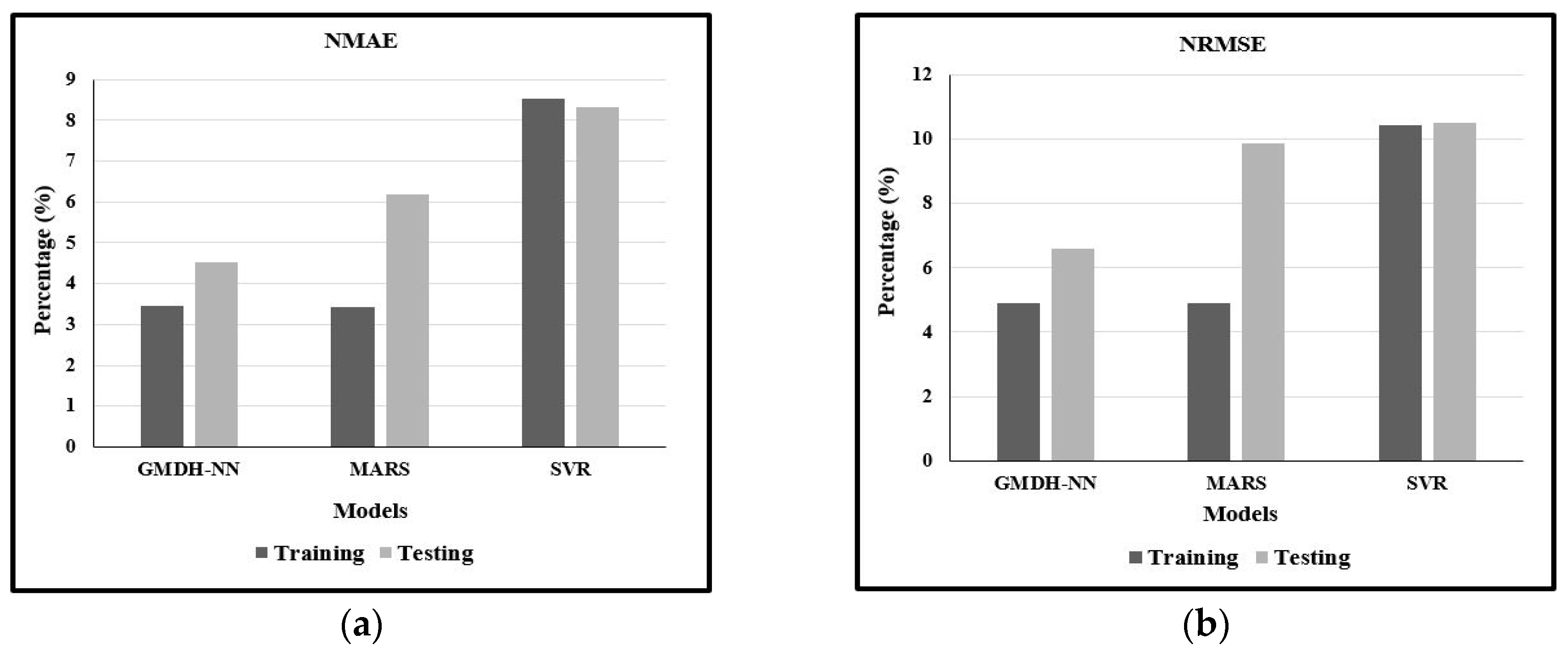
A close value of $R$ to 1, shows a good correlation between the observed and the predicted value of the various model. MAE measures the closeness of the predicted and observed value, while RMSE shows the deviation of a predicted value from the observed value. MAE and RMSE have the unit similar to the dependent input value, i.e., a lower value of predictive variables depicts a better prediction model. An efficiency of 1, (E = 1) corresponds to a perfect match of the model to the observed data and can range from −∞ to 1. The SI is a normalized measure of error, lower value of the SI is an indication of better model performance. For anonymous consideration of the model for the various type of dataset, MAE and RMSE have converted to unitless. So, MAE and RMSE are symbolized as a percentage concerning the difference between the maximum and minimum predicted values, which are the normalized values. The normalization of MAE and RMSE are expressed as NMAE and NRMSE, respectively, which are presented as:

$$NMAE(\%)=\frac{MAE}{max(n)-min(n)}\times 100$$

(34)

$$NRMSE(\%)=\frac{RMSE}{max(n)-min(n)}\times 100$$

(35)

5. Results and Discussion

5.1. Experimental Outcomes

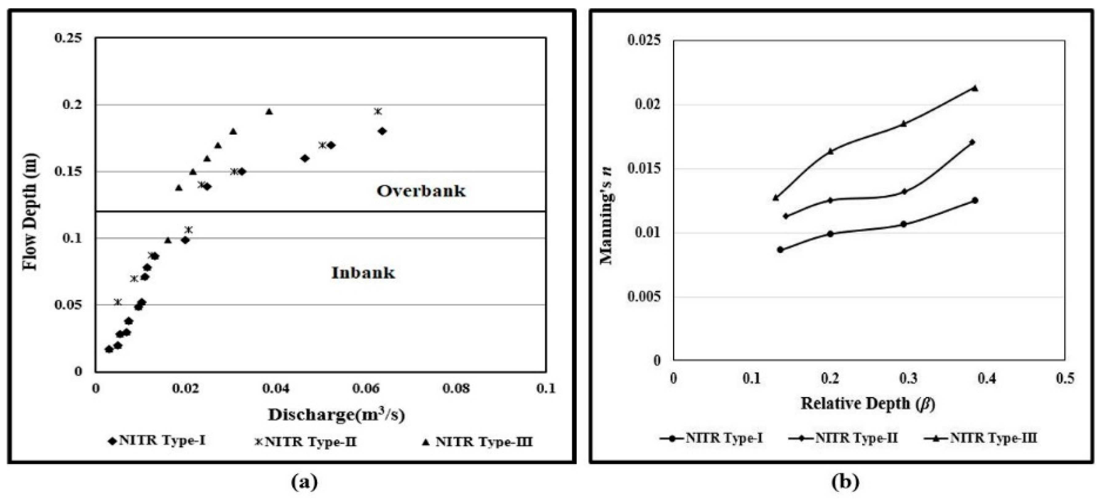
From the experimental data relationship between stage and discharge is shown in Figure 7a. The variation of Manning’s $n$ with the relative depth is presented in Figure 7b. The value of $n$ for overbank flow is found to increase with the increase of relative depth for the compound meandering channels, as shown in Figure 7b. Many investigators [45,68,69] have reported the increasing trend of Manning’s n with the depth of flow.

5.2. Comparison of Predictive Models

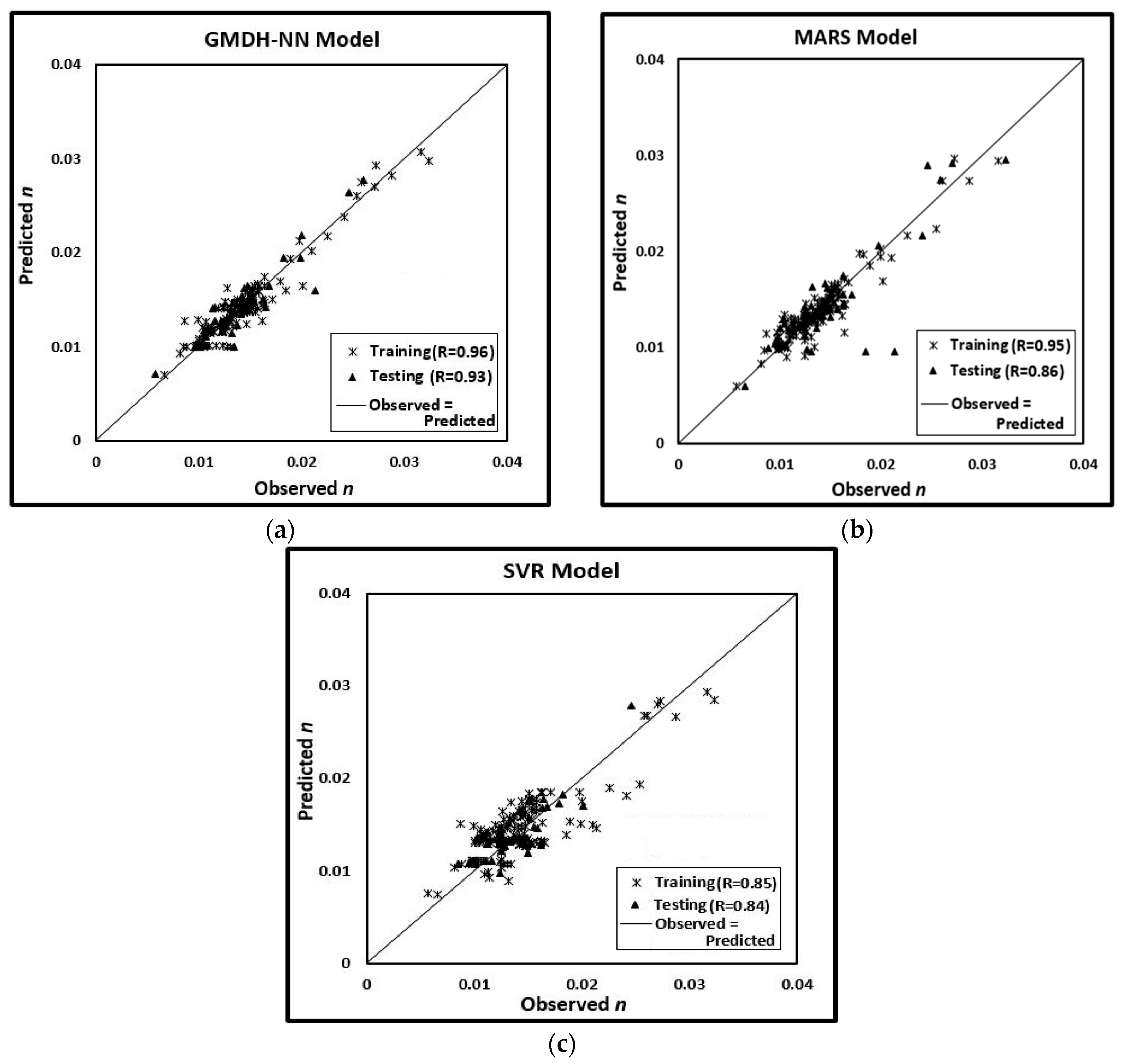
All of the three ML models used in this study shows promising results for predicting Manning’s $n$. Figure 8 shows the scatter plots between the predicted $(n_{pi})$ and the observed $(n_{oi})$ Manning’s $n$. All the three models give acceptable results of Manning’s $n$, which have been seen from Figure 8 as well as

Table 4. Performance Metrics of correlation coefficient (R), mean absolute error (MAE), mean absolute percentage error (MAPE), and root-mean-square-error (RMSE) for GMDH-NN, MARS, and SVR Model.

Index	GMDH-NN		MARS		SVR
	Training	Testing	Training	Testing	Training	Testing
R	0.959	0.932	0.948	0.859	0.846	0.840
MAE	0.0008	0.0009	0.0008	0.0016	0.0019	0.0013
RMSE	0.0012	0.0013	0.0012	0.0025	0.0023	0.0017
MAPE	0.060	0.067	0.061	0.103	0.137	0.107
E	0.92	0.898	0.889	0.709	0.711	0.670
SI	0.083	0.098	0.085	0.171	0.161	0.129

. Between these three models, the GMDH-NN model gives maximum correlation coefficient (R = 0.93) in the testing period as compared to MARS (0.86) and SVR (0.84). Table 4 gives the values of R, RMSE, MAE, and MAPE that are obtained during the training and testing period in the three developed ML models. There is an agreement of Table 4 with the result in Figure 8, GMDH-NN model gives the minimum value of RMSE for training and testing data as 0.0012 and 0.0013, respectively, as compared to the MARS and SVR model. Similarly, when the MAE and the MAPE are taken into account for performance measurement of all three ML models, a similar conclusion is drawn. SI signifies the percentage of difference in root mean square error concerning the mean observation. It gives the percentage of predictable error for parameters. Here, the GMDH model shows lower SI value, which gives the best predicting model. Also, in case of efficiency (E), GMDH-NN gives the least error both in training and testing phase. Similarly, when the MAE and the MAPE are taken into account for performance measurement of all three ML models, a similar conclusion is drawn. As also described in Table 4, the MAPE values indicate that the GMDH-NN model gives the minimum error when compared to the other two models, all through the data series for prediction of $n$. The MAPE values are observed to be less than 7% for GMDH-NN model, whereas the MAPE values of MARS and SVR models greater than 9% in testing phase throughout the range of data. GMDH has been used for the identification of a mathematical model that has many input variables, but limited data needs by using a hierarchical structure [70]. Though we have not studied the computation time of these models used in this study, however various authors reported that SVR models required more time to train [71,72].

For a better comparison of the performances of GMDH-NN, MARS, and SVR model, the normalized value of mean absolute error (NMAE) and root mean square error (NRMSE) is shown in Figure 9a,b, respectively. GMDH-NN gives the lower value of NMAE and NRMSE for testing data, as presented in Figure 9, respectively, concerning the ELM and SVR models. From the figure, it is observed that the GMDH-NN model is superior for calculating Manning’s $n$.

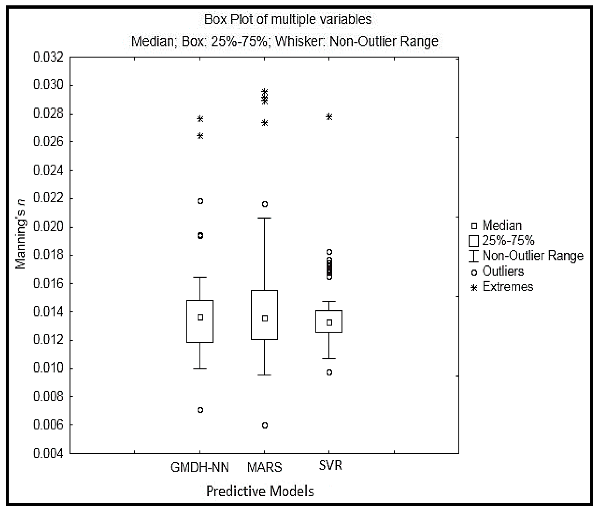
A box and whisker plot, which is used for graphically representing groups of numerical data through their quartiles is shown in Figure 10. In the boxplot, the lower and the upper ends lie at the lower quartile (25th percentile of the dataset $(p_{25})$) and the upper quartile (75th percentile of the dataset $(p_{75})$), respectively. Inside the boxplot, the 50th percentile $(p_{50})$ of the dataset is the median value of the predicted Manning’s $n$. The whisker is the two horizontal lines extended from the uppermost (top) and lowermost (bottom) of the box, whereby the lowermost whisker prolongs from $p_{25}$ to the minimum non-outlier, which is the poorest expected Manning’s $n$ value in the predicted data. The top whisker tracks from $p_{75}$ to the largest non-outlier. Based on graphical representation, the distribution statistics of the lower quartile $(n_{p_{25}})$, median $(n_{p_{50}})$, upper quartile Manning’s $n$ $(n_{p_{75}})$, mean $(\overline{n})$, standard deviation $({\sigma }_n)$, range $(n_{range})$, skewness, and kurtosis $(n_{flat})$ are given in

Table 5. The Distribution Statistics of Predicted Manning’s Coefficient $(n)$ using different Machine learning (ML) Models.

Predictive Model	GMDH-NN	MARS	SVR
(1)	(2)	(3)	(4)
Lower quartile $(n_{p_{25}})$	0.012	0.012	0.013
Median $(n_{p_{50}})$	0.014	0.014	0.013
Upper quartile $(n_{p_{75}})$	0.015	0.015	0.014
Mean $(\overline{n})$	0.014	0.015	0.014
Standard deviation $({\sigma }_n)$	0.004	0.005	0.003
Range $(n_{range})$	0.021	0.024	0.018
Skewness $(n_{skew})$	1.772	1.789	2.56
Kurtosis $(n_{flat})$	4.359	3.285	10.334

. Here, $n$ denotes the predicted value of Manning’s $n$. It is noticed that all of the quartile values obtained seems to be in almost similar range in three models for the predicted $n$. These results are verified with the corresponding values of the distribution statistics, as shown in Table 5. The GMDH-NN model reveals the greatest degree of the range of predicted $n$, which is also justified by the extended bottom-end of the whisker plot, as in Figure 10.

6. Application of the Model to River Data

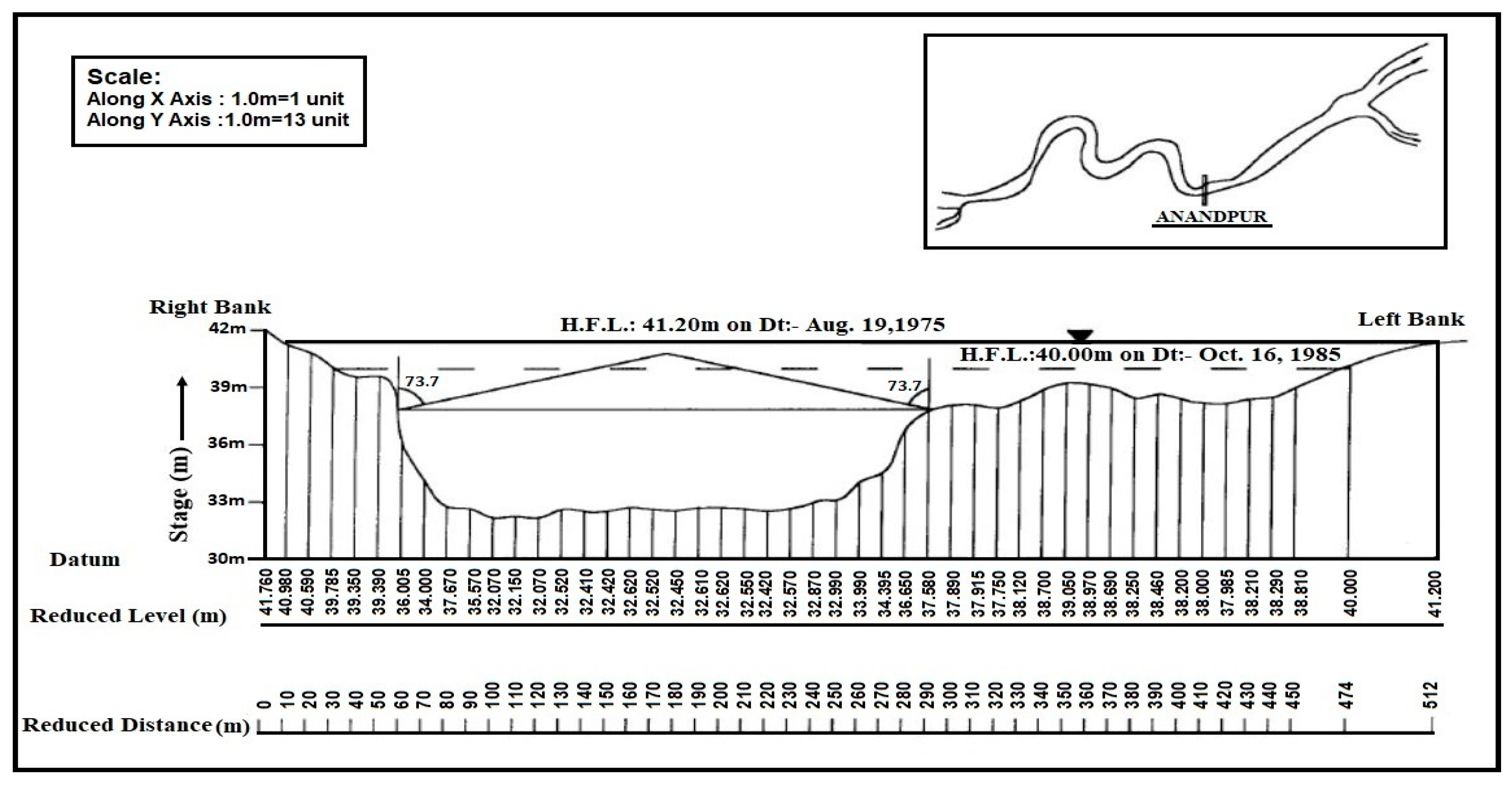
The developed model should be adequate for its practical application, imitating the natural phenomena. The most effective hydraulic experimental solutions may not necessarily be the most globally acceptable solutions. Therefore, the proposed model is applied to river data to know its appropriateness. The Baitarani River is chosen for the application of the developed model for calculation of discharge involving meandering compound channel reach, for 7.5 m depth of flow in the year 1985 flood and 8.63 m depth of flow in the year 1975, which is located between longitude ${86}^{\circ }{8}^{\prime }\mathrm{E}$ and latitude ${20}^{\circ }10^{\prime }\mathrm{N}$ at Anandapur, Odisha, India. Figure 11 shows the plan and cross-sectional view of River Baitarani [44]. At Anandapur site, the river has developed a good meandering plan form with a drainage area of 8570 km². The average bank full depth $(h)$, the width of the main river $(b)$, a top width of the main river $(T)$, sinuosity $(s)$, Meander Belt width $(B_{MW})$, and amplitude $(\epsilon )$ of the river is scaled as 5.4 m, 210 m, 230 m, 1.334, 108 m, and 425 m, respectively. The surface condition for the main channel is sandy, whereas the floodplain has grass vegetation. The average longitudinal slope of the channel bed is 0.0011 for both the floodplain and main river. The river data is collected from Government of India Central Water Commission, Eastern Rivers Division, India.

While using the model equations that are provided by GMDH (Equations (20 through 25)), MARS (Equation (26)), and SVR (Equation (27)) for the evaluation of Manning’s $n$, we need the values of input parameters. For the river Baitarani the values of $\alpha$, $\beta$, $\omega$, $S_o$, $s$ are given in

Table 6. Testing of Model by Predicting Discharge of Baitarani River.

Stage	Flow Depth, H (m)	Width B (m)	$\mathit{\delta }$$(\mathit{b}/\mathit{h})$	$\mathit{\alpha }$$(\mathit{B}/\mathit{b})$	$\mathit{\beta }$$(\mathit{H}-\mathit{h}/\mathit{H})$	$\mathit{\omega }$$({\mathit{B}}_{\mathit{M}\mathit{W}}/\mathit{B})$	$\mathit{r}$$(\mathit{\epsilon }/\mathit{B})$	Observed Q QOBS (m3/s)	Predicted Q (m3/s)
									QGMDH	QMARS	QSVR
40 ${}^a$	7.5	474.6	38.89	2.26	0.28	0.895	0.227	7855	7362.65	8600.76	7022.8
41.2 ${}^b$	8.63	514.5	38.89	2.45	0.374	0.826	0.209	12,200	11,830.7	11,766.7	9307.9

${}^a$ Government of India Central Water Commission, Eastern Rivers Division, (Annual 1985); ${}^b$ Government of India Central Water Commission, Eastern Rivers Division, (Annual 1975).

. By putting the corresponding values in the equations (Equations (20), (26) and (27)), we get the final value of Manning’s $n$ by three models, which can subsequently use to get a discharge in the compound channels. For 7.5 m depth of flow in the river Baitarani, the Manning’s $n$ is calculated by GMDH, MARS, SVR model as 0.0239, 0.0205, and 0.025, respectively. Similarly, for 8.63 m flow depth, the Manning’s $n$ is calculated by GMDH, MARS, SVR model as 0.0242, 0.0201, and 0.0255, respectively. The area of the river is measured as 1995 m², 2485 m² and perimeter as 460 m, 510 m for two different flood flow depth. Subsequently, the values of discharge are estimated by substituting $n$ value in Manning’s general equation. Discharge results that are based on the application of GMDH-NN, MARS, and SVR models are given in Table 6, which indicates the adequacy of the GMDH-NN model.

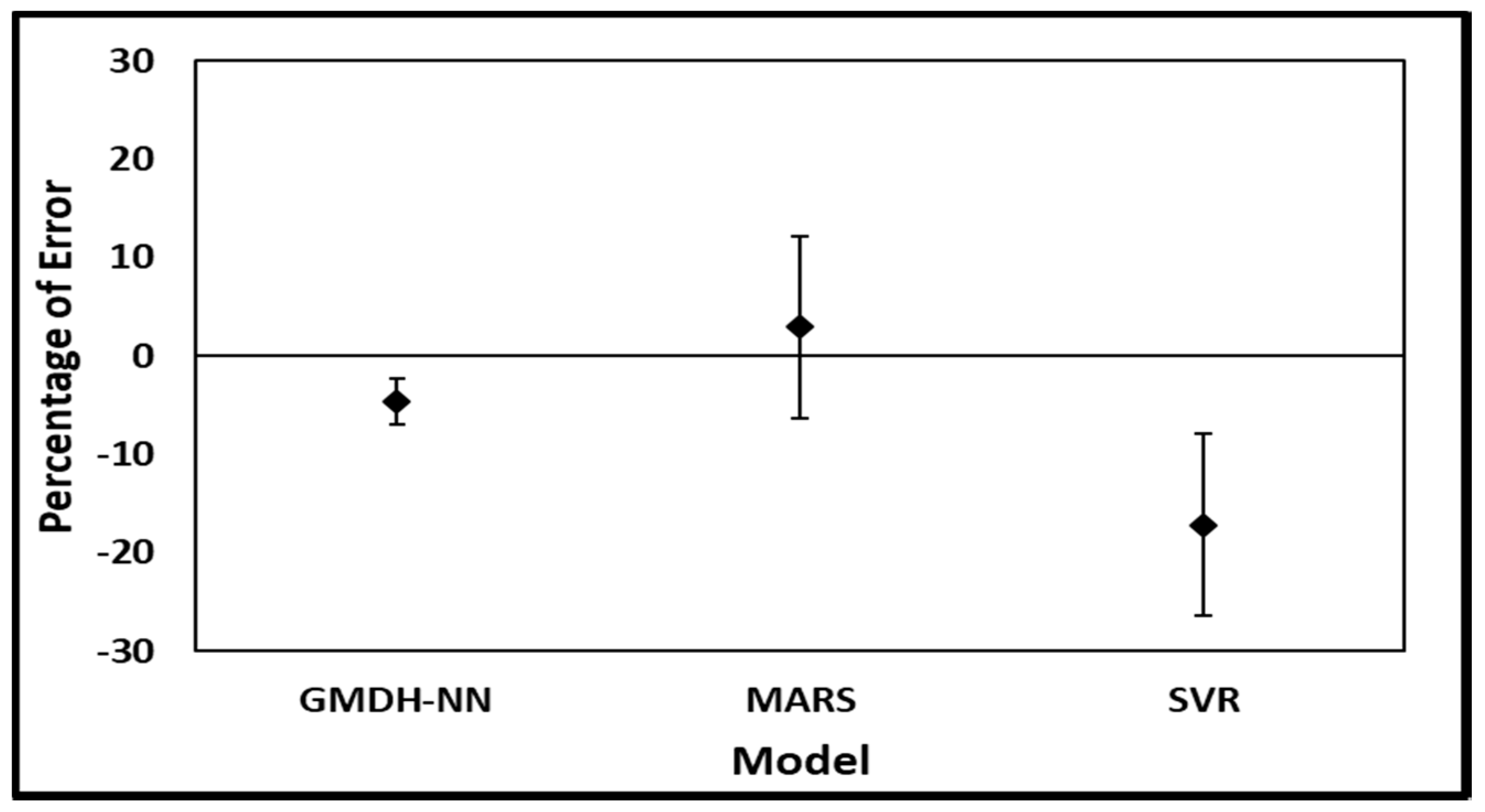
The percentage of mean error for prediction of $n$ by various models and their standard deviation is shown in Figure 12. The authors also accomplished the analysis of inaccuracy in terms of the root-mean-square error (RMSE), mean absolute error (MAE) and mean absolute percentage error (MAPE) as described in

Table 7. Error Analysis of River Baitarani for Prediction of Discharge by Various Models.

Model	GMDH-NN	MARS	SVR
(1)	(2)	(3)	(4)
MAE	430.8	589.5	1862.2
RMSE	435.2	609.9	2128.0
MAPE (%)	4.6	6.5	17.2

for developed models. It is observed that the GMDH-NN model gives the minimum mean percentage error. It is found that the least values of respective MAE, RMSE, and MAPE as 0.00105, 0.00114, and 4.904 for GMDH-NN model. The results give a clear suggestion of the efficiency of the GMDH-NN model and its use in practical applications.

7. Conclusions

The primary interest of this study is to predict the best estimation of Manning’s $n$ for meandering compound channels. Three Artificial Intelligence technics are applied for the modeling of $n$. The fitness of the GMDH-NN model is compared with SVR and MARS machine learning methods. GMDH-NN model has a greater correlation coefficient, smaller error statistics, and fewer outliers, thus showing more promising for predicting Manning’s $n$ as compared to MARS and SVR. From various observations, it can be concluded that the computation time for predicting Manning’s $n$ of GMDH model is the least and also more flexible for data input variables as compared to MARS and SVR model. The models achieved in this study seem to be very useful for the prediction of the Manning’s $n$ of two-stage meandering channels. The model is also applied to the river data for calculating discharge by using the Manning’s equation for its practical implications. For the computing Manning’s $n$ that can hold good for all types of meandering compound channel geometry including the natural rivers irrespective of variation in the beds and floodplain surfaces. Though we have considered smooth channel surface both at the main channel and floodplain, the model is applied very successfully to the Baitarani river data giving minimum error between the computed and observed discharges. The mean percentage error accompanied by the standard deviation for the three models describes the suitability of the model for its field study. The machine-learning model achieved in this study seems to be very useful for the prediction of the Manning’s $n$ of small scale, as well as large-scale models and natural resources.

References

- Azamathulla, H.M.; Ahmad, Z.; Ghani, A.A. An expert system for predicting manning’s roughness coefficient in open channels by using gene expression programming. Neural Comput. Appl. 2013, 23, 1343–1349. [Google Scholar] [CrossRef]
- Bilgil, A.; Altun, H. Investigation of flow resistance in smooth open channels using artificial neural networks. Flow Meas. Instrum. 2008, 19, 404–408. [Google Scholar] [CrossRef]
- Te Chow, V. Open Channel Hydraulics; McGraw-Hill Book Company, Inc.: New York, NY, USA, 1959. [Google Scholar]
- Cowan, W.L. Estimating hydraulic roughness coefficients. Agric. Eng. 1956, 37, 473–475. [Google Scholar]
- Fasken, G.B. Guide for Selecting Roughness Coefficient “N” Values for Channels; US Dept. of Agriculture, Soil Conservation Service: Washington, DC, USA, 1963.
- Limerinos, J.T. Determination of the Manning Coefficient from Measured Bed Roughness in Natural Channels; US Department of the Interior, Geological Survey, Water Resources Division: Menlo Park, CA, USA, 1969.
- Jarrett, R.D. Hydraulics of high-gradient streams. J. Hydraul. Eng. 1984, 110, 1519–1539. [Google Scholar] [CrossRef]
- Arcement, G.J.; Schneider, V.R. Guide for Selecting Manning’s Roughness Coefficients for Natural Channels and Flood Plains; US Government Printing Office: Washington, DC, USA, 1989.
- Yen, B.C. Dimensionally homogeneous manning’s formula. J. Hydraul. Eng. 1992, 118, 1326–1332. [Google Scholar] [CrossRef]
- James, C.S.; Wark, J.B. Conveyance Estimation for Meandering Channels; Report SR 329, Hydraulic Res; HR Wallingford Ltd.: Wallingford, UK, 1992. [Google Scholar]
- Shiono, K.; Al-Romaih, J.S.; Knight, D.W. Stage-discharge assessment in compound meandering channels. J. Hydraul. Eng. 1999, 125, 66–77. [Google Scholar] [CrossRef]
- Jena, S. Stage-Discharge Relationship in Simple Meandering Channels. Master’s Thesis, Indian Institute of Technology (IIT), Kharagpur, India, 2007. [Google Scholar]
- Mailapalli, D.R.; Raghuwanshi, N.S.; Singh, R.; Schmitz, G.H.; Lennartz, F. Spatial and temporal variation of manning’s roughness coefficient in furrow irrigation. J. Irrig. Drain. Eng. 2008, 134, 185–192. [Google Scholar] [CrossRef]
- Khatua, K.K.; Patra, K.C.; Mohanty, P.K. Stage-discharge prediction for straight and smooth compound channels with wide floodplains. J. Hydraul. Eng. 2012, 138, 93–99. [Google Scholar] [CrossRef]
- Khatua, K.K.; Patra, K.C.; Nayak, P. Meandering effect for evaluation of roughness coefficients in open channel flow. WIT Trans. Ecol. Environ. 2012, 146, 213–224. [Google Scholar]
- Khatua, K.K.; Patra, K.C.; Nayak, P.; Sahoo, N. Stage-discharge prediction for meandering channels. Int. J. Comput. Methods Exp. Meas. 2013, 1, 80–92. [Google Scholar] [CrossRef]
- Xia, J.; Lin, B.; Falconer, R.A.; Wang, Y. Modelling of man-made flood routing in the lower yellow river, china. Proc. Inst. Civ. Eng. 2012, 165, 377–391. [Google Scholar] [CrossRef]
- Barati, R.; Akbari, G.H.; Rahimi, S. Flood routing of an unmanaged river basin using muskingum–cunge model; field application and numerical experiments. Casp. J. Appl. Sci. Res. 2013, 2, 8–20. [Google Scholar]
- Barati, R. Application of excel solver for parameter estimation of the nonlinear muskingum models. KSCE J. Civ. Eng. 2013, 17, 1139–1148. [Google Scholar] [CrossRef]
- Barati, R.; Rahimi, S.; Akbari, G.H. Analysis of dynamic wave model for flood routing in natural rivers. Water Sci. Eng. 2012, 5, 243–258. [Google Scholar]
- Dash, S.S.; Khatua, K.K. Sinuosity dependency on stage discharge in meandering channels. J. Irrig. Drain. Eng. 2016, 142, 04016030. [Google Scholar] [CrossRef]
- Pradhan, A.; Khatua, K.K. Assessment of roughness coefficient for meandering compound channels. KSCE J. Civ. Eng. 2017, 1–13. [Google Scholar] [CrossRef]
- Zhang, M.; He, C.; Liatsis, P. A d-gmdh model for time series forecasting. Expert Syst. Appl. 2012, 39, 5711–5716. [Google Scholar] [CrossRef]
- Mrugalski, M. An unscented kalman filter in designing dynamic gmdh neural networks for robust fault detection. Int. J. Appl. Math. Comput. Sci. 2013, 23, 157–169. [Google Scholar] [CrossRef]
- Najafzadeh, M.; Lim, S.Y. Application of improved neuro-fuzzy gmdh to predict scour depth at sluice gates. Earth Sci. Inform. 2015, 8, 187–196. [Google Scholar] [CrossRef]
- Vapnik, V. Pattern recognition using generalized portrait method. Autom. Remote Control 1963, 24, 774–780. [Google Scholar]
- Boser, B.E.; Guyon, I.M.; Vapnik, V.N. A training algorithm for optimal margin classifiers. In Proceedings of the Fifth Annual Workshop on Computational Learning Theory, Pittsburgh, PA, USA, 27–29 July 1992; pp. 144–152. [Google Scholar]
- Cortes, C.; Vapnik, V. Support-vector networks. Mach. Learn. 1995, 20, 273–297. [Google Scholar] [CrossRef] [Green Version]
- Gualtieri, J.A.; Chettri, S.R.; Cromp, R.F.; Johnson, L.F. Support vector machine classifiers as applied to aviris data. In Proceedings of the Eighth JPL Airborne Geoscience Workshop, Pasadena, CA, USA, 8–11 February 1999. [Google Scholar]
- Vapnik, V. Statistical Learning Theory; Wiley: New York, NY, USA, 1998; Volume 3. [Google Scholar]
- Dibike, Y.B.; Velickov, S.; Solomatine, D.; Abbott, M.B. Model induction with support vector machines: Introduction and applications. J. Comput. Civ. Eng. 2001, 15, 208–216. [Google Scholar] [CrossRef]
- Pal, M.; Goel, A. Prediction of the end-depth ratio and discharge in semi-circular and circular shaped channels using support vector machines. Flow Meas. Instrum. 2006, 17, 49–57. [Google Scholar] [CrossRef]
- Han, D.; Chan, L.; Zhu, N. Flood forecasting using support vector machines. J. Hydroinform. 2007, 9, 267–276. [Google Scholar] [CrossRef] [Green Version]
- Genc, O.; Dag, A. A machine learning-based approach to predict the velocity profiles in small streams. Water Resour. Manag. 2016, 30, 43–61. [Google Scholar] [CrossRef]
- Samui, P.; Das, S.; Kim, D. Uplift capacity of suction caisson in clay using multivariate adaptive regression spline. Ocean Eng. 2011, 38, 2123–2127. [Google Scholar] [CrossRef]
- Samui, P.; Kurup, P. Multivariate adaptive regression spline (mars) and least squares support vector machine (lssvm) for ocr prediction. Soft Comput. 2012, 16, 1347–1351. [Google Scholar] [CrossRef]
- Samui, P. Multivariate adaptive regression spline (mars) for prediction of elastic modulus of jointed rock mass. Geotech. Geol. Eng. 2013, 31, 249–253. [Google Scholar] [CrossRef]
- Knight, D.W.; Shiono, K. Turbulence measurements in a shear layer region of a compound channel. J. Hydraul. Res. 1990, 28, 175–196. [Google Scholar] [CrossRef]
- Shiono, K.; Knight, D.W. Turbulent open-channel flows with variable depth across the channel. J. Fluid Mech. 1991, 222, 617–646. [Google Scholar] [CrossRef]
- Toebes, G.H.; Sooky, A.A. Hydraulics of meandering rivers with flood plains. J. Waterw. Harb. Div. 1967, 93, 213–236. [Google Scholar]
- Kar, S.K. A Study of Distribution of Boundary Shear in Meander Channel with and without Floodplain and River Floodplain Interaction. Ph.D. Thesis, Indian Institute of Technology Kharagpur, Kharagpur, India, 1977. [Google Scholar]
- Das, A.K. A Study of River Flood Plain Interaction and Boundary Shear Stress Distribution in a Meander Channel with One Sided Flood Plain. Ph.D. Thesis, Indian Institute of Technology Kharagpur, Kharagpur, India, 1984. [Google Scholar]
- Kiely, G.K. An Experimental Study of Overbank Flow in Straight and Meandering Compound Channels. Ph.D. Thesis, Department of Civil Engineering, University College, Cork, Ireland, 1989. [Google Scholar]
- Patra, K.C.; Kar, S.K. Flow interaction of meandering river with floodplains. J. Hydraul. Eng. 2000, 126, 593–604. [Google Scholar] [CrossRef]
- Khatua, K.K. Interaction of Flow and Estimation of Discharge in Two Stage Meandering Compound Channels. Ph.D. Thesis, National Institute of Technology Rourkela, Odisha, India, 2007. [Google Scholar]
- Mohanty, P.K. Flow Analysis of Compound Channels with Wide Flood Plains Prabir. Ph.D. Thesis, National Institute of Technology Rourkela, Odisha, India, 2013. [Google Scholar]
- Ervine, D.A.; Willetts, B.B.; Sellin, R.H.J.; Lorena, M. Factors affecting conveyance in meandering compound flows. J. Hydraul. Eng. 1993, 119, 1383–1399. [Google Scholar] [CrossRef]
- Moharana, S.; Khatua, K.K. Prediction of roughness coefficient of a meandering open channel flow using neuro-fuzzy inference system. Measurement 2014, 51, 112–123. [Google Scholar] [CrossRef]
- Amanifard, N.; Nariman-Zadeh, N.; Farahani, M.H.; Khalkhali, A. Modelling of multiple short-length-scale stall cells in an axial compressor using evolved gmdh neural networks. Energy Convers. Manag. 2008, 49, 2588–2594. [Google Scholar] [CrossRef]
- Ivakhnenko, A.G. Polynomial theory of complex systems. IEEE Trans. Syst. Man Cybern. 1971, 4, 364–378. [Google Scholar] [CrossRef]
- Ivakhnenko, A.G.; Ivakhnenko, G.A. Problems of further development of the group method of data handling algorithms. Part I. Pattern Recognit. Image Anal. 2000, 10, 187–194. [Google Scholar]
- Farlow, S.J. Self-Organizing Methods in Modeling: Gmdh Type Algorithms; CRC Press: Boca Raton, FL, USA, 1984; Volume 54. [Google Scholar]
- Sanchez, E.; Shibata, T.; Zadeh, L.A. Genetic Algorithms and Fuzzy Logic Systems: Soft Computing Perspectives; World Scientific: Singapore, 1997; Volume 7. [Google Scholar]
- Iba, H.; deGaris, H.; Sato, T. A numerical approach to genetic programming for system identification. Evolut. Comput. 1995, 3, 417–452. [Google Scholar] [CrossRef]
- Friedman, J.H. Multivariate adaptive regression splines. Ann. Stat. 1991, 19, 1–67. [Google Scholar] [CrossRef]
- Friedman, J.H.; Roosen, C.B. An Introduction to Multivariate Adaptive Regression Splines; Sage Publications: Thousand Oaks, CA, USA, 1995. [Google Scholar]
- Leathwick, J.R.; Rowe, D.; Richardson, J.; Elith, J.; Hastie, T. Using multivariate adaptive regression splines to predict the distributions of new zealand’s freshwater diadromous fish. Freshw. Biol. 2005, 50, 2034–2052. [Google Scholar] [CrossRef]
- Craven, P.; Wahba, G. Smoothing noisy data with spline functions. Numer. Math. 1978, 31, 377–403. [Google Scholar] [CrossRef]
- Vapnik, V.N. The Nature of Statistical Learning Theory; Springer: Berlin, Germany, 1995. [Google Scholar]
- Vapnik, V.N. An overview of statistical learning theory. IEEE Trans. Neural Netw. 1999, 10, 988–999. [Google Scholar] [CrossRef] [PubMed]
- Osuna, E.; Freund, R.; Girosi, F. An improved training algorithm for support vector machines. In Proceedings of the 1997 IEEE Workshop Neural Networks for Signal Processing VII, Amelia Island, FL, USA, 24–26 September 1997; pp. 276–285. [Google Scholar] [Green Version]
- Gunn, S.R. Support vector machines for classification and regression. ISIS Tech. Rep. 1998, 14, 5–16. [Google Scholar]
- Smola, A.J. Regression Estimation with Support Vector Learning Machines. Master’s Thesis, Technische Universität München, München, Germany, 1996. [Google Scholar]
- Jia, X.; Zhao, M.; Di, Y.; Yang, Q.; Lee, J. Assessment of data suitability for machine prognosis using maximum mean discrepancy. IEEE Trans. Ind. Electron. 2018, 65, 5872–5881. [Google Scholar] [CrossRef]
- Thissen, U.; Pepers, M.; Üstün, B.; Melssen, W.J.; Buydens, L.M.C. Comparing support vector machines to pls for spectral regression applications. Chemom. Intell. Lab. Syst. 2004, 73, 169–179. [Google Scholar] [CrossRef]
- Gandomi, A.H.; Yun, G.J.; Alavi, A.H. An evolutionary approach for modeling of shear strength of rc deep beams. Mater. Struct. 2013, 46, 2109–2119. [Google Scholar] [CrossRef]
- Ebtehaj, I.; Bonakdari, H.; Zaji, A.H.; Azimi, H.; Khoshbin, F. Gmdh-type neural network approach for modeling the discharge coefficient of rectangular sharp-crested side weirs. Eng. Sci. Technol. Int. J. 2015, 18, 746–757. [Google Scholar] [CrossRef]
- Knight, D.W.; Hamed, M.E. Boundary shear in symmetrical compound channels. J. Hydraul. Eng. 1984, 110, 1412–1430. [Google Scholar] [CrossRef]
- Patra, K.C. Flow Interaction of Meandering River with Flood Plains. Ph.D. Thesis, Indian Institute of Technology Kharagpur, Kharagpur, India, 1999. [Google Scholar]
- Hwang, H.-S.; Bae, S.-T.; Cho, G.-S. Container terminal demand forecasting framework using fuzzy-gmdh and neural network method. In Proceedings of the Second International Conference on Innovative Computing, Informatio and Control, Kumamoto, Japan, 5–7 September 2007; p. 119. [Google Scholar]
- Sun, J.; Cho, S. Pattern selection for support vector regression based on sparseness and variability. In Proceedings of the International Joint Conference on Neural Networks (IJCNN’06), Vancouver, BC, Canada, 16–21 July 2006; pp. 599–602. [Google Scholar]
- Wardaya, P.D. Support vector machine as a binary classifier for automated object detection in remotely sensed data. IOP Conf. Ser. Earth Environ. Sci. 2014, 18, 1–6. Available online: http://iopscience.iop.org/article/10.1088/1755-1315/18/1/012014/meta (accessed on 16 July 2018). [CrossRef]
Figure 1.
Geometric Configuration of Meandering Compound Channel (National Institute of Technology Rourkela (NITR) Type-I).
Figure 2.
Geometric Configuration of Meandering Compound Channel (NITR Type-II).
Figure 3.
Geometric Configuration of Doubly Meandering Compound Channel (NITR Type-III).
Figure 4.
Plan View of the Experimental Meandering Compound Channel.
Figure 5.
Photograph of Experimental Channel Setup (a) NITR Type-I Channel; (b) NITR Type-II Channel; and, (c) NITR Type-III Channel.
Figure 6.
Grid Arrangement of Points for experimental measurements across the channel section.
Figure 7.
The relationship of (a) Stage-discharge for experimental channels; and (b) Manning’s with relative depth.
Figure 8.
The Scatter Plots show the Regression Coefficient and the 1:1 Perfect Fit Line between the Observed and Predicted Manning’s for (a) Group Method of Data Handling Neural Network GMDH-NN) Model; (b) MARS Model; and (c) support vector machine regression (SVR) Model.
Figure 9.
Performance of Training and Testing Data Samples for Prediction of by (a) normalized value of mean absolute error (NMAE); and (b) root mean square error (NRMSE).
Figure 10.
Performances Statistics Established for the Prediction of Manning’s using developed GMDH-NN, MARS, and SVR Model.
Figure 11.
Cross-section of Baitarani River at the gaging site (Anandapur, Odisha, India) [44].
Figure 12.
Percentage of Error of Discharge for River Baitarani for Prediction values by the three Models.