Modeling of GRACE-Derived Groundwater Information in the Colorado River Basin


1
Department of Civil and Environmental Engineering, Southern Illinois University, 1230 Lincoln Drive, Carbondale, IL 62901, USA
2
Department of Civil and Environmental Engineering and Construction, University of Nevada, Las Vegas, NV 89154, USA
*
Author to whom correspondence should be addressed.
Hydrology 2019, 6(1), 19; https://doi.org/10.3390/hydrology6010019
Submission received: 30 December 2018
/
Revised: 25 January 2019
/
Accepted: 17 February 2019
/
Published: 18 February 2019
(This article belongs to the Special Issue Remote Sensing in Hydrological Modelling)
Abstract
:Groundwater depletion has been one of the major challenges in recent years. Analysis of groundwater levels can be beneficial for groundwater management. The National Aeronautics and Space Administration’s twin satellite, Gravity Recovery and Climate Experiment (GRACE), serves in monitoring terrestrial water storage. Increasing freshwater demand amidst recent drought (2000–2014) posed a significant groundwater level decline within the Colorado River Basin (CRB). In the current study, a non-parametric technique was utilized to analyze historical groundwater variability. Additionally, a stochastic Autoregressive Integrated Moving Average (ARIMA) model was developed and tested to forecast the GRACE-derived groundwater anomalies within the CRB. The ARIMA model was trained with the GRACE data from January 2003 to December of 2013 and validated with GRACE data from January 2014 to December of 2016. Groundwater anomaly from January 2017 to December of 2019 was forecasted with the tested model. Autocorrelation and partial autocorrelation plots were drawn to identify and construct the seasonal ARIMA models. ARIMA order for each grid was evaluated based on Akaike’s and Bayesian information criterion. The error analysis showed the reasonable numerical accuracy of selected seasonal ARIMA models. The proposed models can be used to forecast groundwater variability for sustainable groundwater planning and management.
1. Introduction
The portion of water stored in pore spaces of soil and rock beneath the Earth’s surface is known as groundwater. Groundwater is a major and dependable large source of freshwater for domestic, agricultural, and industrial users in all climatic regions of the world [1,2]. It also plays a central role to maintain the balance in the ecosystem [3,4]. The areas with highly variable rainfall fully depend on groundwater due to lack of adequate alternative resources of fresh water. The over-exploitation of groundwater is a threat to the sustainability of ecosystems, water supply, and economic and social developments [5]. More energy is needed to pump out the dwindling groundwater levels, which triggers higher energy consumption [6]. Ground subsidence may also occur for the excessive groundwater depletions [7,8]. Long-term sustainable groundwater from river basins has become a major concern among scientists. It is difficult to quantify the rate of natural renewal of groundwater to subsidize the water table depletion required for supporting the ecosystem [9]. A proper understanding of groundwater storage (GWS) variation at spatial and temporal scale helps to understand the hydrologic cycle and its effect on global climate change. Therefore, consistent monitoring of the groundwater levels and storage may help to develop better plans for maintaining balanced ecosystems, sustainable economic development and encountering the water stress [10].
Routine monitoring of groundwater from regional to continental scale with the networks of monitoring well is tedious, time-consuming, and expensive. The inconsistency in data collection at the temporal scale, scarce of evenly distributed monitoring wells, the complicated subsurface physical properties, and recharging processes make the groundwater head estimation more complicated. Sometimes to access the hydrological data is restricted by the law enforcement agency. Since 1970s scientists are working on satellite-based remote-sensing systems for measuring hydrological component; groundwater is the latest addition on that [11]. Avoiding aforementioned challenges, National Aeronautics and Space Administration (NASA)’s twin Gravity Recovery and Climate Experiment (GRACE) mission provides the first opportunity to directly measure groundwater changes from space through the accurate estimation of Earth’s gravity field variations over time and space [12,13,14]. Unlike traditional remote sensors utilizing electromagnetic emissions, GRACE uses K-Band microwave to estimate inter-satellite drift due to the gravitational force, the effect of the redistribution of earth mass component including cryosphere, hydrosphere, ocean, atmosphere, and land surface within the accuracy of a micrometer. The GRACE data is processed with numerical models to truncate the effect of atmospheric and oceanic contributions. Therefore, GRACE-observed mass changes mostly reflect terrestrial water storage (TWS), vertical integration of groundwater, soil moisture (SM), surface water (SW), snow water, and vegetation water measurements. Removing the change in surface water storage from GRACE gravity measurements yields an estimated change in groundwater [6,15,16,17,18]. GRACE provides groundwater level variability relative to the user-defined time baseline instead of an optimal value of groundwater level from the surface or any datum. GRACE-derived GWS demonstrated higher potential to represent the in-situ groundwater-level [18,19,20,21]. Many studies have already quantified groundwater variability from GRACE gravity measurements [22,23,24].
Analyzing the historical variability of the GRACE-derived GWS will help to understand future groundwater conditions. Trend analysis is one of the popular and most accepted methods of analyzing the variability of any data and is also popular while analyzing the changes in a hydrologic variable [25,26,27]. Hydro-meteorological data are often non-normally distributed where mean does not represent the central tendencies as effectively as the median. In such cases, non-parametric tests are often useful over parametric tests to analyze the time series data. Mann–Kendall (MK) a commonly used non-parametric statistical test to detect the trend in hydro-meteorological data [25,26,28]. MK test was introduced by Kendall, [29] and Mann, [30] and is thus named after them. It is the rank-based trend detection analysis which gives the statistical significance of the trend if they are present in the time series. Further, the magnitude of the trend is often evaluated with the Thiel-Sen approach in most of the time series analysis [26,28,31].
Modeling and predicting of groundwater level fluctuation provides valuable information regarding groundwater declination, trend and allowable limit of exploitation. Forecasting the potential change in groundwater levels can help to mitigate the issues associated with water management [32]. Accurate prediction of groundwater head helps planners to augment urban, rural, and industrial freshwater demand. Groundwater level forecasting also helps to comprehend the dynamics between factors that affect groundwater tables. An accurate and reliable groundwater forecasting helps to develop integrated management of groundwater and SW [5]. The comprehensive river basin management policies require a continuous water level assessment, modeling, and forecasting. Over the past years, the conceptual and physically-based numerical models are widely used in groundwater simulation and quantification. These models are able to replicate the physical properties of groundwater dynamics. However, these modeling techniques have practical limitations due to the absence of long-term high- quality data and the complex structures of aquifers [33,34,35,36]. In such cases, statistics-based time series analysis can be used as a suitable alternative [33,37]. The time series analysis is able to deal with the data that are collected at a regular interval, like groundwater measurements. Time series analysis is widely used in groundwater resources management [38,39,40,41].
The prediction process in time series analysis highly depends on previous observations. Among various statistical approaches, a stochastic process is commonly used to capture the trend of forecasted data considering uncertainty. Autoregressive Integrated Moving Average (ARIMA) model is one of the most popular models that follow the behavior of the stochastic process [42]. ARIMA and autoregressive moving average model (ARMA) is often utilized to understand and forecast different time series data. Unlike ARMA, ARIMA model is beneficial while working with the non-stationary time series data. ARIMA model considers the underlying correlation and patterns in the lagged data to forecast future data. ARIMA is the combination of differencing, auto-regression (AR), and moving average (MA) technique. The ARIMA deals with the fewer coefficients, which is the foremost benefit of using this model. ARIMA is the mathematical approach for predicting the future scenario considering the changes in trends and serial correlation among the previous observations. The use of the ARIMA model to forecast the hydrological time series data are well documented. In hydro-climatological research, the ARIMA model was used for predicting the mean monthly streamflow [43,44], rainfall [39,45], long-term runoff [46], river water quality and discharge [47,48], and drought [49].
The need for sustainable decisions through groundwater assessment and prediction has motivated the current study. The inconsistency of in-situ groundwater data and the sparseness of such data at higher spatiotemporal scale motivated utilizing the GRACE-derived groundwater anomaly in the current study. Additionally, deterministic forecasting models can mimic the spatial variability of groundwater while they undergo parametric uncertainties resulting in poor forecasts. Thus, to subside such shortcomings, GRACE-derived groundwater anomaly was coupled with ARIMA model for forecasting groundwater anomaly. The study was tested in one of the drought-affected area— the Colorado River Basin (CRB). The Colorado River is governed by the ‘Law of River’ and suffered severe water stress during recent climate change and increasing water demand. Addition to surface water, decline the reductions in groundwater storage was observed. The study tests the following research questions:
- (1)
- Is GRACE-derived data applicable to analyze the groundwater variability in the region undergoing drought like CRB?
- (2)
- What are the historic spatiotemporal variations in the groundwater in the CRB?
- (3)
- Can a stochastic ARIMA model coupled with GRACE data forecast future groundwater variability at the selected spatiotemporal scale of the CRB?
The aforementioned research questions are addressed by utilizing GRACE-derived groundwater changes as such data provides a longer length of data at uniform spatiotemporal scales. Before using the GRACE data for further study, it was tested against the in-situ observations to verify its reliability. The spatiotemporal variability of the historic GRACE-derived groundwater anomaly was tested using non-parametric MK test, and the magnitude of the trend was analyzed with Thiel-Sen’s approach. Then, the stochastic ARIMA model was developed by determining its parameters to accommodate the seasonality and autocorrelation in the groundwater. Finally, the ARIMA model was tested to simulate the historical and future groundwater variability in the CRB. The documented research reveals that significant efforts had been made in the past to forecast groundwater conditions especially in the regions with higher water stress. According to documented literature and the author’s knowledge, this is the first time ARIMA is integrated with GRACE data to predict future groundwater anomalies. ARIMA model showed promising result while simulating historical groundwater records, which can be utilized for groundwater management. Associating the proposed model with other deterministic models may enhance the confidence of both approaches. This novel approach may help water managers in making sustainable groundwater policies.
2. Study Area
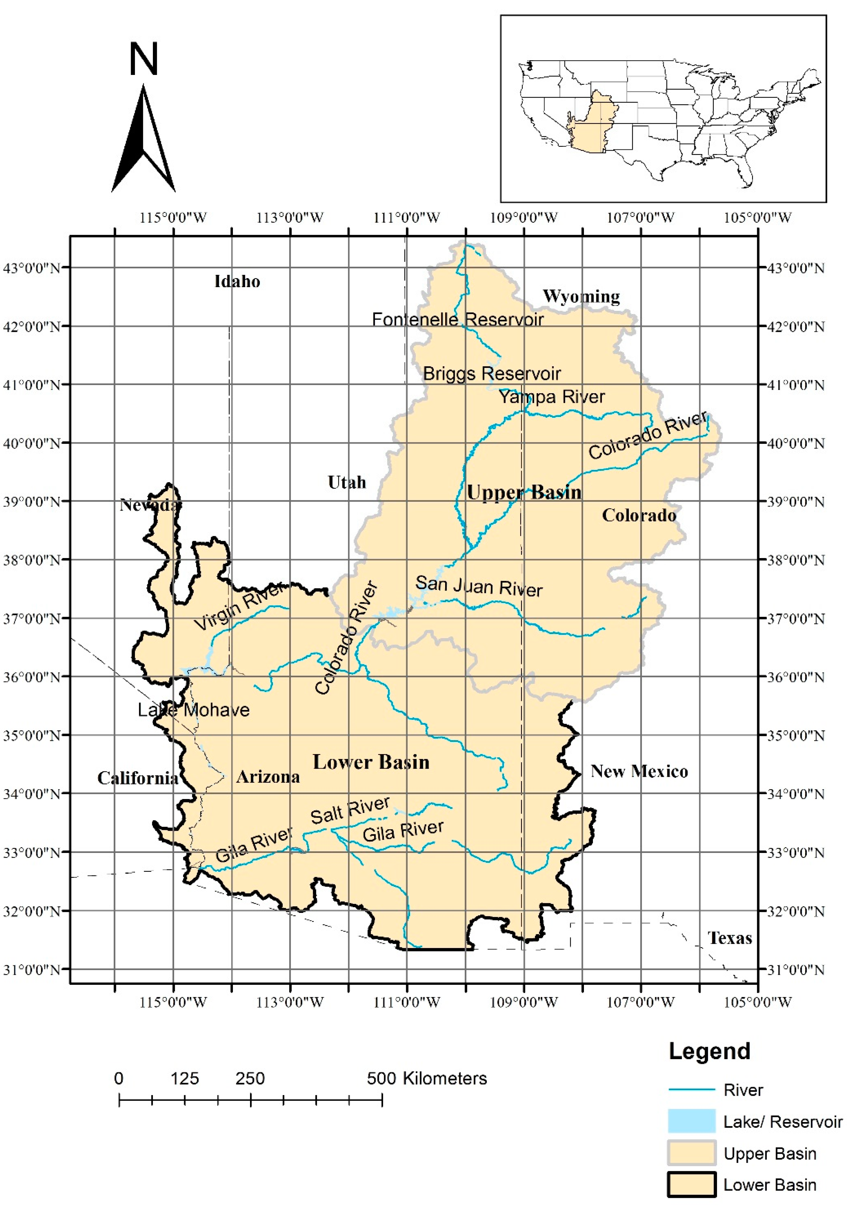
The study area comprising of CRB including major rivers is illustrated in Figure 1. CRB has an area of 657,000 km2 which sources water supply to approximately 40 million people of seven different states (Colorado, Utah, Nevada, Arizona, California, Wyoming, and New Mexico), and Mexico [50]. CRB is divided into the lower CRB and upper CRB, where 8.6 million and 1 million people reside respectively [51]. Streams mostly originate in the upper part of the basin approximately ninefold as compared to the lower part. This basin provides water to a total of 22,000 km2 of irrigated land [50]. Population growth and increased irrigation in the CRB has boosted water consumption. Increasing water demands and severe drought since 2000 have posed the declination of water levels in the CRB’s largest reservoirs–Lake Powell and Lake Mead. To offset paucity of surface water supplies in drought, water users have switched to using groundwater to a greater extent. But the irregularities of groundwater reserves in CRB raises questions: how much water is already consumed, and how long can it be sustained? Castle et al. (2014) [52] showed that the CRB experienced a loss of 41 million acre-feet groundwater from 2003 to 2014, 77 percent of total freshwater decrement. Groundwater pumping for irrigation triggered the losses in water storage [53]. Groundwater is being depleted at a much faster rate than previously thought indicating that the CRB is going to experience a groundwater decline in the coming years.
3. Data Sources
The data sets used in the analysis comprises of GRACE and Global Land Data Assimilation System (GLDAS) data [54]. Section 3.1 provides details about the GRACE data followed by Section 3.2 which discusses how different hydrologic components of water balance equation were obtained from GLDAS data. Section 3.2 also presents the assimilation of GRACE and GLDAS data to calculate groundwater storage anomaly.
3.1. GRACE Data
GRACE is twin satellite launched by the NASA, and the German Aerospace Centre combined in March 2002 for tracking down the mass redistribution of the earth by monitoring changes in gravitational force [14]. As GRACE record cumulative signals both gravitational and non-gravitational effects, atmospheric and oceanic effect need to be isolated to quantify the change in hydrological mass [55,56]. GRACE provides monthly data at both 1° × 1° [57] and 0.5° × 0.5° [58] spatial resolution. To reduce noise and measurement errors, several filtering processes such as a destriping filter, a 200 km wide Gaussian averaging filter, and the low-pass spectral filter are applied [13]. The filtering process for getting smoother data weakens true geophysical signals. A set of scaling factors is considered with the data set to restore the signal [59]. The present study uses GRACE Level-3 RL 05 anomaly data, with temporal and spatial resolution of one month and of 1° × 1° respectively, obtained from the Center for Space Research at the University of Austin/Texas (CSR), NASA Jet Propulsion Laboratory (JPL) and the German Research Centre for Geosciences (GFZ) to calculate GWS variations. While computing the equivalent water height, the average of CSR, JPL, and GFZ was taken to reduce the noise [21]. The time series of variability in gravity field for each cell from January 2003 to July 2016 were used in this study. This dataset has gaps of several months. The imputeTS [60], an R package, was used to take care of missing values as the ARIMA model cannot deal with the time series with missing data [61]. The TWS comprises GWS, SM, SW, snow water equivalent (SWE), and canopy water storage (CWS). The scaling factor was used to restore the information of the GRACE-derived product, ignoring the effect of the SW component [62]. The change in TWS was calculated using the water balance equation as shown in Equation (1).
where, , , , , and represent the change in TWS, GWS, SM, SWE, and CWS respectively.
3.2. Global Land Data Assimilation System (GLDAS)
GLDAS is a joint project of NASA, the National Oceanic and Atmospheric Administration, and the National Centers for Environmental Prediction which simulate hydrologic components by integrating ground-based and satellite observations at a higher temporal and spatial resolution [54]. GLDAS provides hydrological data using four Land Surface Models (LSMs), i.e., the Community Land Model (CLM) [63], Variable Infiltration Capacity (VIC) [64], Noah [65], and Mosaic [66]. To measure the changes in GWS from GRACE TWS, the values of SM, SWE, and CWS need to be deducted from the land surface model of GLDAS. The average of four LSMs models (CLM, VIC, Noah, and Mosaic) was used to calculate the anomaly of SM, SWE, and CWS to minimize any biases or errors [20]. All LSMs with a similar spatial and temporal resolution of GRACE was used in this study. The GLDAS derived products (SM, SWE, and CWS) were also converted to the same anomaly of GRACE.
SM/SWE/CWS anomaly at time t, was evaluated as shown in Equation (2).
where P represents SM/SWE/CWS and represents corresponding average P from January 2004 to December 2009. Finally, groundwater storage anomalies (GWSA) was calculated utilizing Equation (3) shown below.
The in-situ groundwater head was obtained from monitoring stations, which was a measure of relative height from North American Vertical Datum of 1988. Groundwater level change from different monitoring wells was factored by respective specific yield to get GWS. Then, GWSA from the observed value was calculated using the same equation used for GLDAS data. This GWSA had been evaluated in terms of change in groundwater level represented hereafter as ΔGWL. Adjusted ΔGWL from in-situ was compared with GRACE-derived ΔGWS.
4. Methodology
First, Section 4.1 discusses the evaluation of historical variations in groundwater storage. Followed by Section 4.2 which presents the method of forecasting groundwater anomaly with the ARIMA model.
4.1. Evaluation of Trend in the Groundwater Data
MK—a rank-based test—was utilized to detect the presence of the trend in the GRACE-derived ΔGWS data. The test also revealed the statistical significance of the trend if any in each gridded data. More details on the MK test can be obtained from Mann [30] and Kendall [29]. The current study only considered the trend if they were detected at 5% statistical significance based on the MK test. The trend magnitude was calculated utilizing the Theil-Sen approach [31].
4.2. ARIMA Model
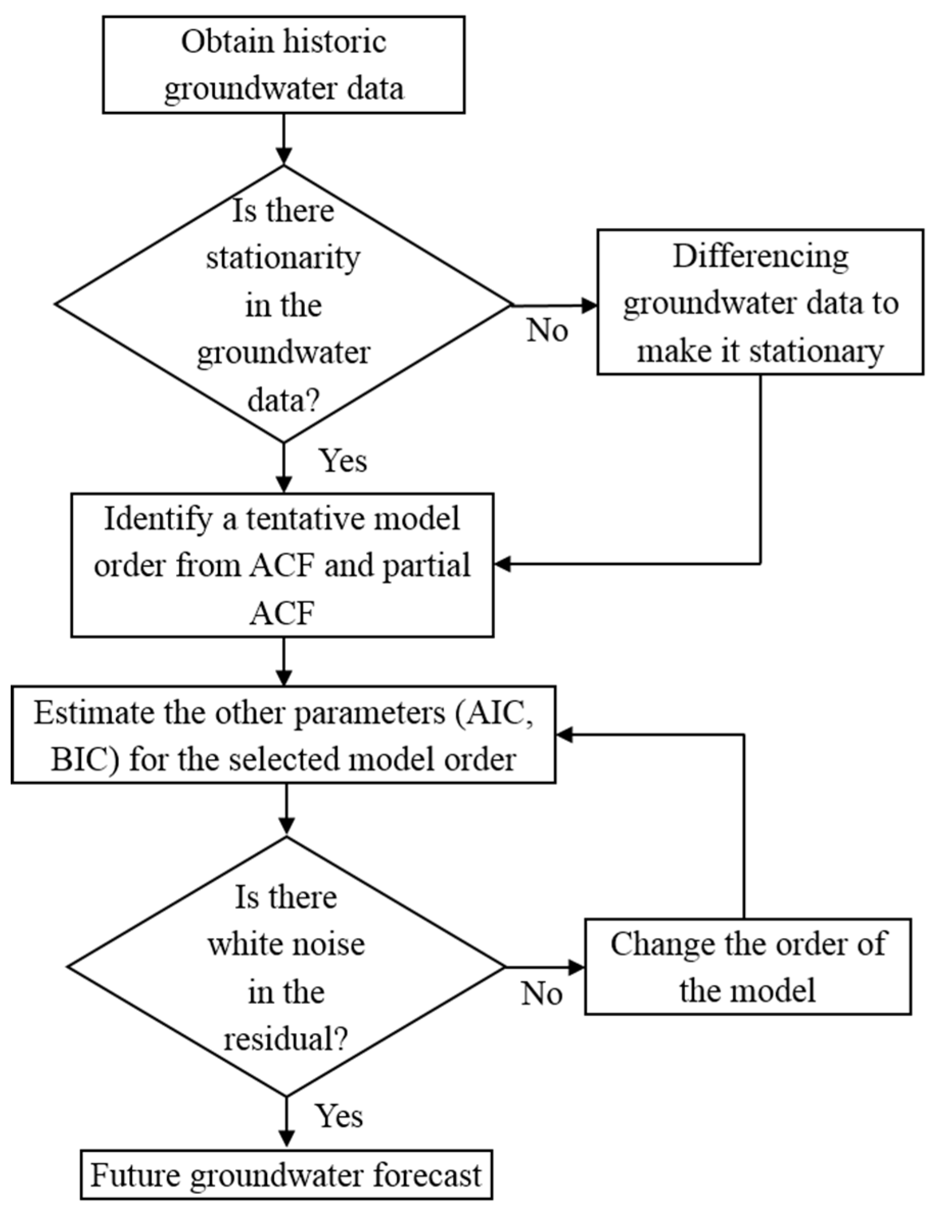
The ARIMA model framework is shown in Figure 2. First, the groundwater data was procured as presented in Section 3. Figure 2 illustrates the steps involved in developing an ARIMA model corresponding to the GRACE-derived groundwater anomaly of one grid which was repeated for the groundwater analysis of entire CRB. As shown in Figure 2, first the groundwater anomaly was derived from the GRACE data which was tested for the presence of stationarity. ARIMA model parameters were derived from the stationary data and if the data was not stationary it was derived from the differenced data. Once, accurate model parameters were obtained, the historical inputs were then utilized to forecast the groundwater anomaly. The equations involved in building an ARIMA model is discussed later in this section.
Before evaluating the model parameters, stationarity in the data was evaluated. Differencing was done to make the data stationary, and the process was accomplished for each grid as shown in Figure 1. The non-seasonal ARIMA model with first-order differencing is expressed as Equation (4) shown below.
where, c is constant, εt is white noise and φ1, φ2……. φn is autoregressive coefficients, and θ1, θ2………θq is the moving average coefficients. Similarly, is the first order differencing obtained by subtracting from and so on.
In general, an ARIMA model is represented as ARIMA (p, d, q) where, p, d, and q are the order of autoregression, integration (differencing), and moving average order, respectively. The more simplified ARIMA model is mathematically expressed as shown in Equation (5) where B is the backward shift operator.
Most of the hydrological data follow a seasonal pattern, like monthly, quarterly etc. The autocorrelation function (ACF) and partial autocorrelation function (PACF) test were performed to determine the seasonality in the dataset. A time series data, attribute with the seasonality, is converted to stationary in nature with the help of seasonal differencing. A seasonal ARIMA model is classified as an ARIMA (p,d,q) (P,D,Q)m model, where P = order of the seasonal autoregression, D = order of seasonal differencing, Q = order of moving average and m = the number of periods in one season.
For the backward shift operator, B, a seasonal ARIMA (p,d,q) (P,D,Q)m can be expressed as follows:
where, φp(B) is Auto regressive operator, θq(B) is moving average operator, Φp(Bm) is Seasonal autoregressive operator, and Θq(Bm) = Seasonal moving average operator.
ARIMA models require stationary time series data for modeling. The stationarity of the input time series data needs to be identified first. If the data series has any non-stationarity component, the non-stationarity should be removed before utilizing the data as ARIMA model inputs. The ACF and PACF plots are used to recognize if a time series exhibits non-stationary or not. ACF shows the correlations between time series and its own lag. PACF also depicts the correlations between the time series and its own lag along with neglecting the effect members stay in between them. The two parallel lines, with the x-axis, in the plots remarks 95% confidence intervals (CI) for the calculated ACF and PACF. Besides an additive seasonal decomposition is performed to visualize the seasonal patterns of time series data.
An additive seasonal decomposition can be written as
where at any period t, seasonal component is represented by St, Tt is the trend component, and
Rt is the remainder component
Differencing is usually used to stationarize the nonstationary data time series. The lowest differencing order for which time series maintain a well-defined mean value and ACF plot decays rapidly to zero, either from above or below, is the appropriate order for differencing. ACF and PACF generally give an idea of tentative order for moving average and autoregressive of ARIMA model. Different order of combinations close to the potential model was generated.
Akaike Information Criterion (AIC) and Bayesian Information Criterion (BIC) were utilized to choose the appropriate ARIMA model. Equations (8) and (9) below present the expressions to evaluate AIC and BIC.
where the sum of squared errors represented by SSE is calculated as . K is parameters in the statistical model, N is the observations number and ε represents the white noise. The minimum values of these AIC and BIC criteria signify better model performance [67].
The errors in the model are often accessed with the residuals. Residuals are random in nature which cannot be explained by mathematical interpretations such as distribution with zero mean and constant variance. They are uncorrelated and normally distributed. ACF and PACF of the residuals are standard evaluation criteria for ARIMA model evaluation. For normally distributed residuals, all the spikes in ACF and partial ACF should range within the threshold values [68]. The fitted model with minimum ACF and PACF for each gridded data were used to forecast the groundwater anomalies.
5. Results and Discussion
5.1. Historical Variations in Groundwater
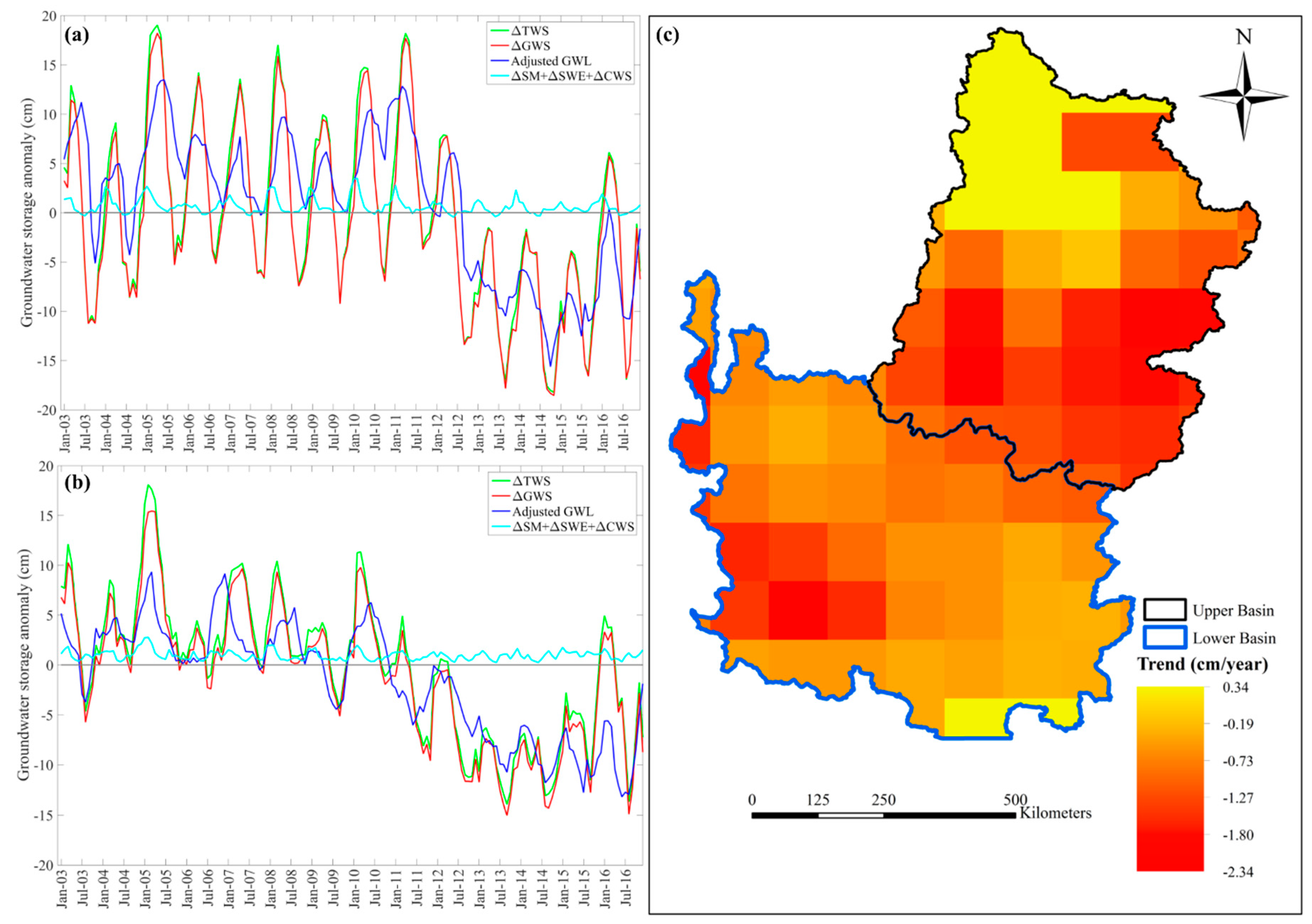
Figure 3a,b represent the monthly time series of GRACE-derived ΔTWS, ΔSM, ΔSWE, and ΔWCS, after taking the average from four GLDAS LSMs, from January 2003 to December 2016 for the both Upper and Lower Colorado River Basin. Equation (3) was used to estimate the monthly distributed groundwater storage anomalies based on GRACE using the above-mentioned hydrological components. GRACE-derived ΔGWS was correlated with the average of in-situ measurements in both upper and lower CRB with the R2 value of 0.62 and 0.67 respectively. The R2 values testify good conformity between satellite and ground-based measurement as for such analysis the R2 between 0.55 and 0.75 is ranked as good correlation [21]. Like previous studies, the larger study area leads to getting better co-relation among GRACE and in-situ observations.
From Figure 3a, it can be observed that the groundwater storage in the upper basin declined sharply during 2013. This can be attributed to the lowest recorded snowfall in Rocky Mountain and extreme drought scenario in 2012 [52]. In lower CRB as observed in Figure 3b, groundwater storage followed a decreasing trend from 2004 to 2012 before it experienced a significant depletion from 2012 to mid-2014. On the other hand, the rise in groundwater storage was visible for a shorter period between mid-2009 to mid-2010). Moderately wetted weather lessened the demand for surface water supplies and groundwater recharged during this period. The consistency in groundwater head, in both upper and lower basin, after January 2015 shows strong evidence of recovery from the drought starting from 2000 up to 2014.
Figure 3c shows the spatial variation of the trend at the statistical significance of p ≤ 0.05. The magnitude of the trend was calculated as the Theil-Sen’s slope is represented in color on the map. The trend magnitude was computed for each grid independently as shown in the figure. This magnitude represents the change in the GRACE-derived ΔGWS in centimeters per year (cm/year). The negative trend magnitude suggests the decline in ΔGWS over time while the positive trend magnitude signifies the increase in ΔGWS over time. As evident from Figure 3c, most of the grid (80 grids out of 94 grids) had shown the significant decline in ΔGWS at the statistical significance of p ≤ 0.05. The maximum negative trend magnitude observed in the CRB was 2.34 cm/year. Thirteen grids did not show any trend at the statistical significance of p ≤ 0.05, and only one grid of lower CRB showed the increase in ΔGWS at the statistical significance of p ≤ 0.05 with the trend magnitude of 0.34 cm/year. As observed in Figure 3c, although entire CRB has experienced a decline in ΔGWS, upper CRB has undergone more decline in the ΔGWS as compared to the ΔGWS of lower CRB. This might be attributed to the recent management and conservation policies in the lower CRB and varying recharge of upper and lower CRB [69]. The decline in ΔGWS deems the assessment of the future groundwater variability in the region.
5.2. ARIMA Model Results
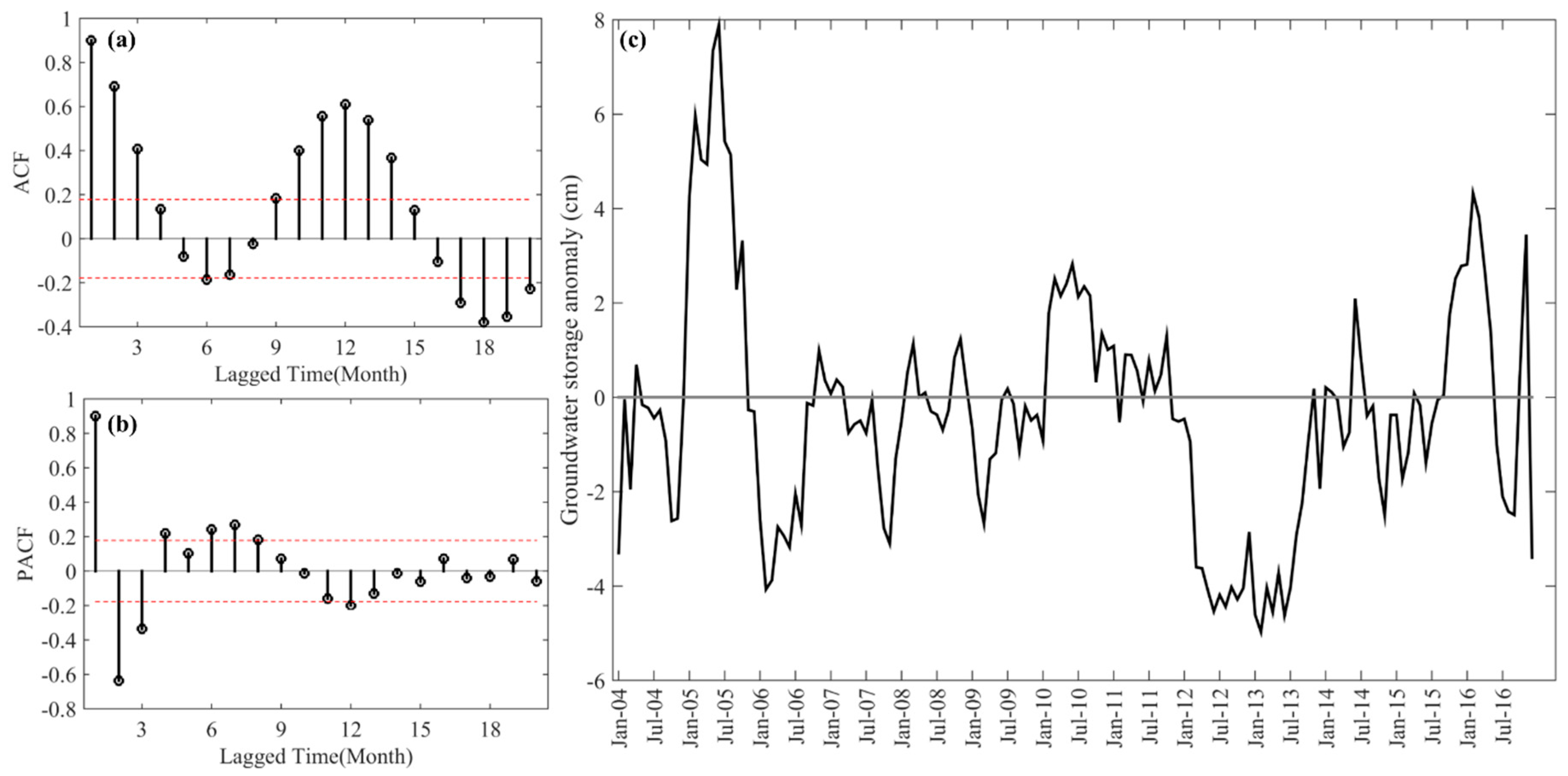
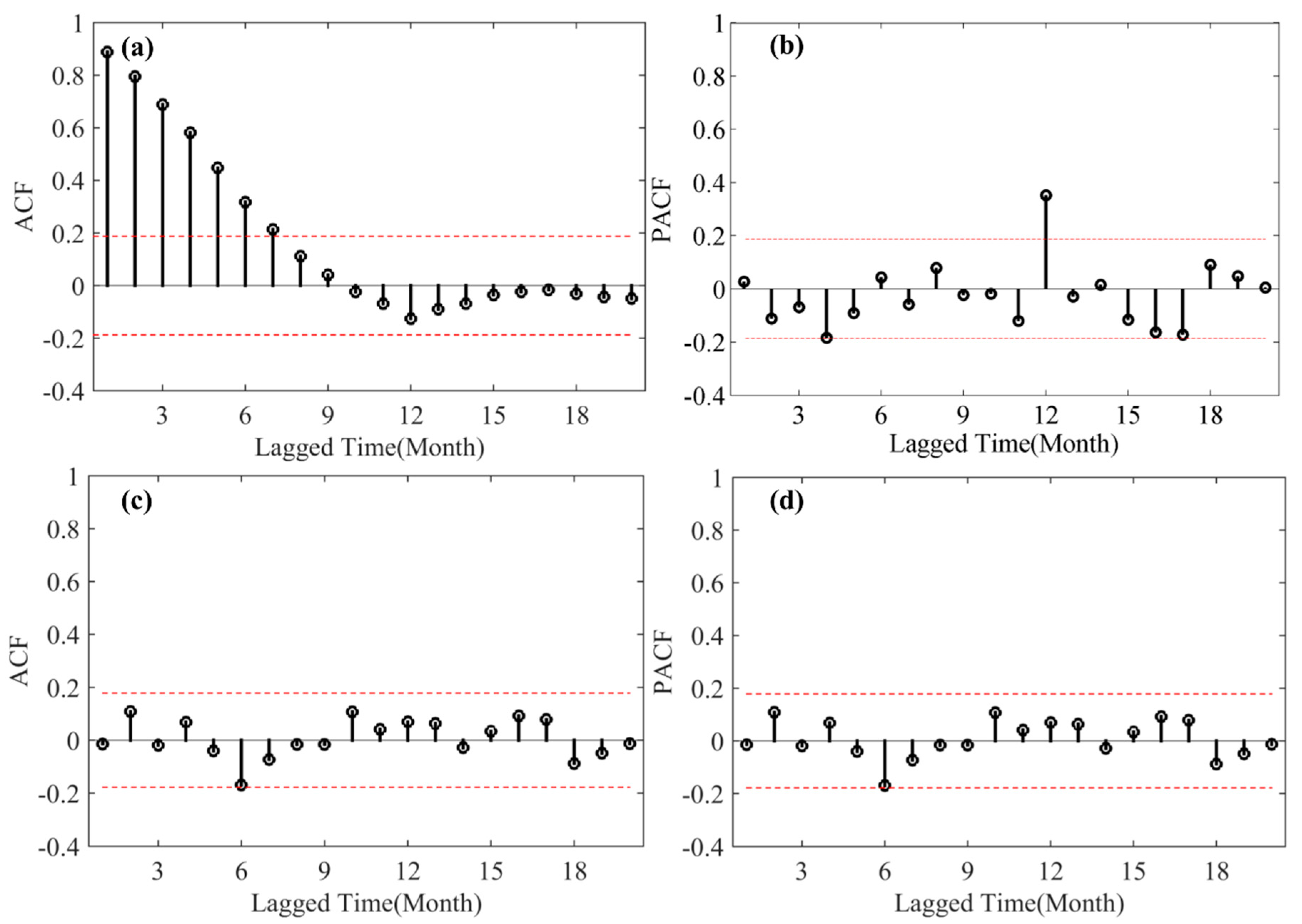
The ARIMA model project future ΔGWS data based on the past trend in GRACE-derived ΔGWS. Selecting the order of ARIMA model is an iterative process which is discussed in the later part of the paper. The absence of constant mean, variance, and autocorrelation over time make the time series data non-stationary. Generally, the non-stationarity appears in two aspects, i.e., changes in the parameters and the feature of the driving cause. Both are difficult to be identified without the prior assumed way the non-stationarity happens. Thus, the stationarity of time series data should be tested before performing any further analysis. First, the intermediate sample results of ARIMA forecast corresponding to the grid with centroid 110.5 ° W and 31.5 ° N referred hereafter as sample grid is presented. After presenting the results corresponding to the sample grid the results pertaining to all grids of CRB are presented. The ACF and PACF correlograms are drawn in order to determine the stationarity in monthly ΔGWS data as shown in Figure 4a,b. Two dotted horizontal red lines in the figure signify the margins at 95% CI for calculated autocorrelation and partial autocorrelation values. Here the horizontal axis (x-axis) shows the lagged time steps while the vertical axis denotes the correlation values for the corresponding lags. As seen in the figure, all the correlation values lie between +1 and −1, the maximum and minimum value respectively.
If the ACF and PACF promptly converge to zero with the increase in the time lag, the time series is considered to be stationary. As seen in Figure 4a, the spikes in the ACF plot are over the threshold values, and their net values are decreasing with time. This prominently indicates the presence of non-stationarity in the groundwater. Besides, the spikes in the PACF plot don’t shut off immediately. In the PACF plot of Figure 4b, several numbers of spikes are above the threshold. This indicates the presence of seasonality in the data. After the occurrence of a trend or non-homogeneity, the time series changes its regime and no longer remains stationary. It is hard to model such non-stationary time series; thus the stationary part of the time series should be extracted before creating any model. ARIMA is associated with the difficulty to model and forecast the time series which are subjected to any changes in the regime. Therefore, 12-month differencing was applied to make it stationary by removing the seasonal influence. The seasonally differenced time-series data are shown in Figure 4c.
Figure 5a,b shows the ACF and PACF plots for seasonally differenced time series corresponding to the sample grid. These plots provide a tentative order of the ARIMA model. The ARIMA model with the tentative order is termed hereafter as the sample model. From Figure 5a, tentative model order cannot be obtained as the higher number of spikes are above the threshold in the ACF plot. There is no significant spike in the PACF as shown in Figure 5b plot for non-seasonal lags, suggesting a possible MA model of zero order. Whereas, for the seasonal component, there is a significant spike at lag 12 signifying the first order seasonal AR corresponding to the sample grid. From this, a preliminary seasonal ARIMA (p, 0, q) (1, 1, 0)12—the potential model was selected to simulate the inter-annual variability GRACE-derived ΔGWS from January of 2003 to December of 2014. In total twelve models corresponding to the sample grid, with several combinations of orders were assumed, close to the tentative order to estimate ARIMA model parameters. The comparison of AIC and BIC of different models are summarized in Table 1. As shown in the table, all the model has the same orders of differencing, as the model was selected minimizing AIC and BIC [70]. Among all models, ARIMA (1,0,1) (1,1,1)12 showed the minimum AIC and BIC. Residual analysis of a fitted model depicts the robustness of the model. For a well-fitted model, the residuals should behave as white noise (random). The ACF and PACF of ARIMA (1,0,1) (1,1,1)12 model residuals for the sample grid are plotted in Figure 5c,d respectively. As shown in Figure 5c,d, spikes of both ACF and PACF, lies within 95% confidence level, indicating the randomness in residuals. Besides, as all the lags have coefficients below the threshold, the absence of autocorrelation between them is confirmed.
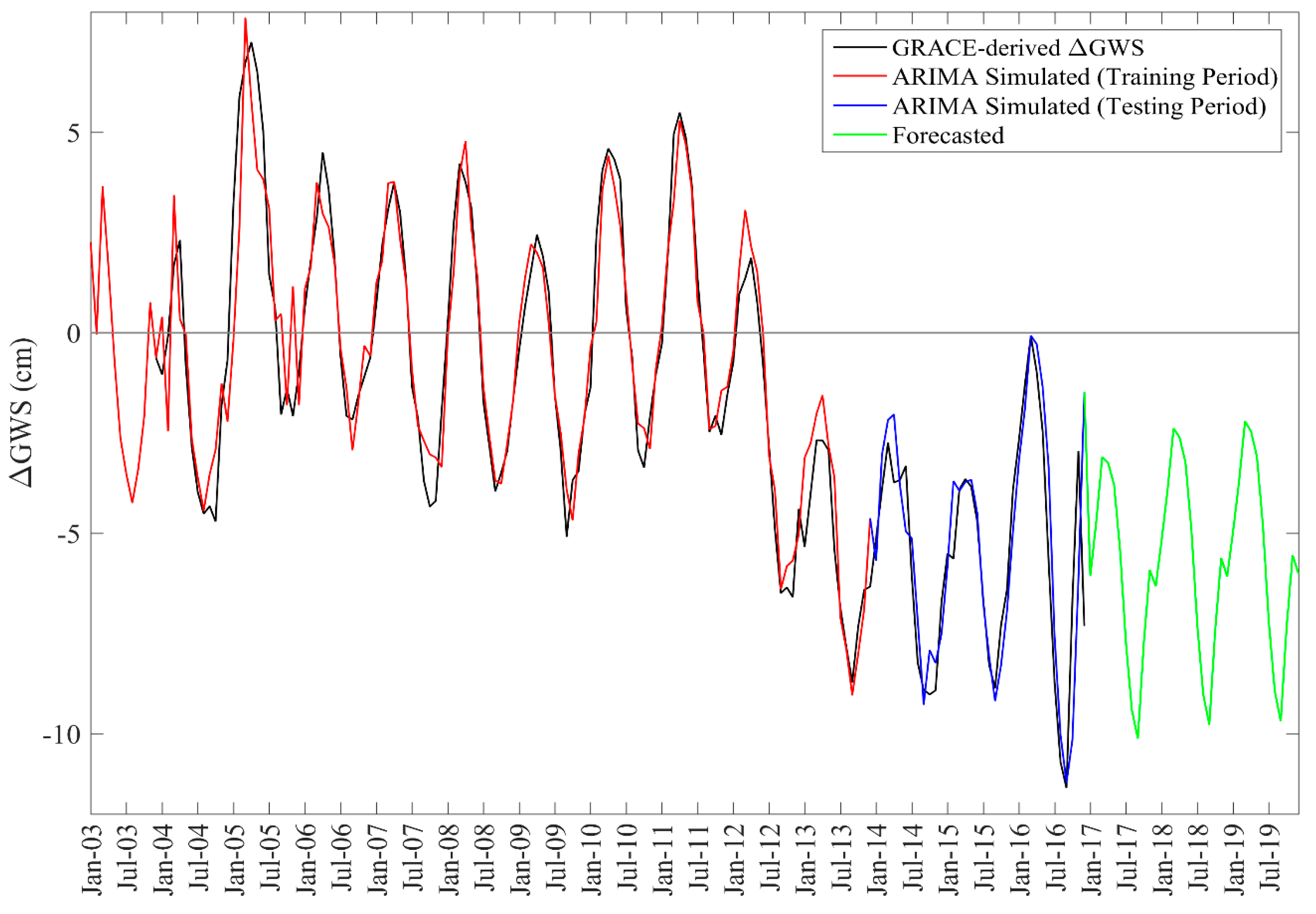
Figure 6 depicts the time series plots of ARIMA simulations along with the GRACE-derived monthly ΔGWS for the sample grid. The model training period (January 2003 to December 2014) clearly illustrates the periodicity of existing GRACE-derived ΔGWS. As shown in Figure 6, the ARIMA model forecasts were close to the GRACE-derived ΔGWS during the testing period (January 2015–December 2016) signifying good model skills. The model also captured the seasonality and the trend of ΔGWS series remarkably well during the testing period as shown in Figure 6. In the training period, the simulated ΔGWS followed the decreasing trend of 0.43 cm/year which was close to the decreasing trend of GRACE-derived ΔGWS evaluated as 0.47 cm/year. On the other hand, during the testing period, both ARIMA results and GRACE-derived ΔGWS showed the recharge in groundwater. Tillman et al. [71] used Coupled Model Intercomparison Project Phase 5 climate projections and supported the idea of recharge in groundwater storage of the CRB. It was observed that the model captured most of the peaks with some minor exceptions. The incompetence of the model to capture some of the peaks may be attributed to the presence of randomness component in the stochastic model. The selected seasonal ARIMA model generates the groundwater storage variability with higher accuracy for the remaining time series. The higher value of Nash–Sutcliffe efficiency (NSE) (0.89) and comparatively lower Root Mean Square Error (RMSE) (1.04) during the training period and 0.72, 1.5 during testing period respectively, indicating higher conformity between satellite-derived and simulated groundwater anomaly for the sample grid. This also suggests robustness of the seasonal ARIMA model that offer anticipated consistency and accuracy. Finally, the tested ARIMA model was utilized to forecast future groundwater anomaly of the sample grid for 36 months.
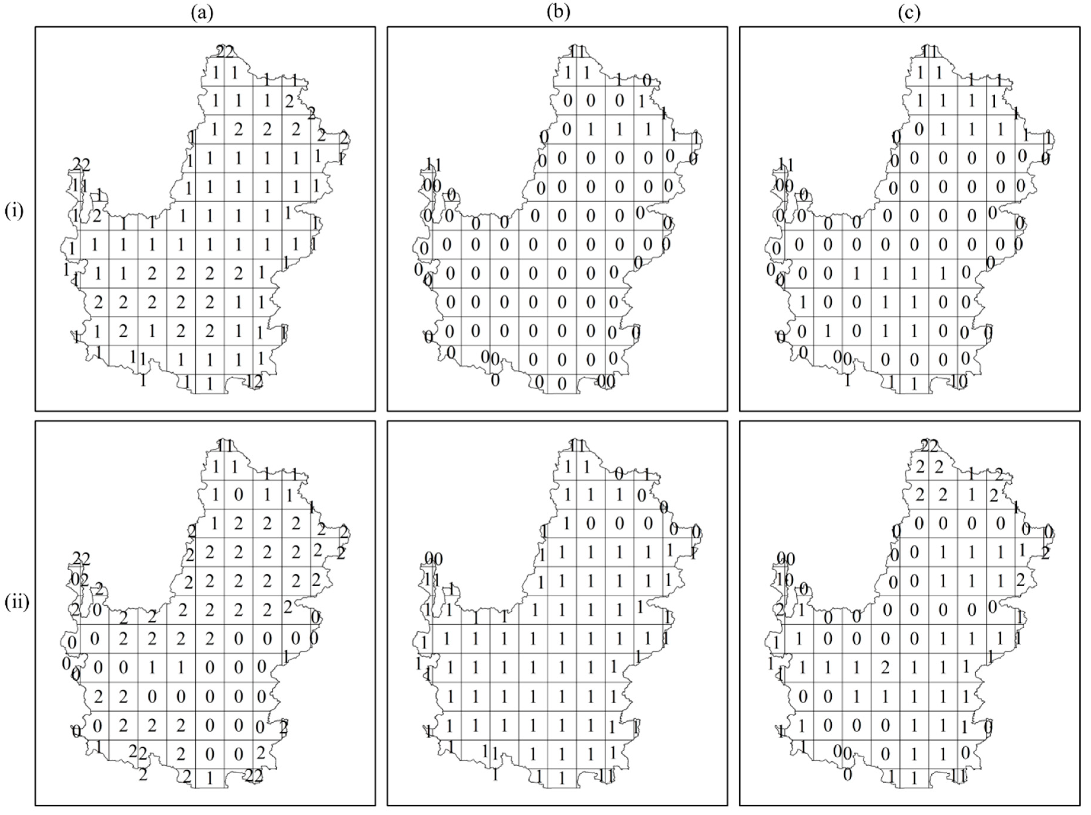
Similar to the sample grid, the analysis was performed for each grid corresponding to the GRACE data within the CRB. Figure 7 shows the distribution of ARIMA model orders for each grid within the CRB. Figure 7i,ii represents the non-seasonal and seasonal components of the ARIMA model respectively. In Figure 7, columns (a), (b), and (c) represents autoregressive order, differencing order, and moving average order respectively. It can be seen that the moving average and autoregressive order both in seasonal and no-seasonal part varies between 0 and 2. The differencing order for the seasonal part was found 1 in almost all the grids. Non-seasonal differencing order was adopted as 1 if the seasonal differencing order was 0 and 0 if the seasonal differencing order was 1.
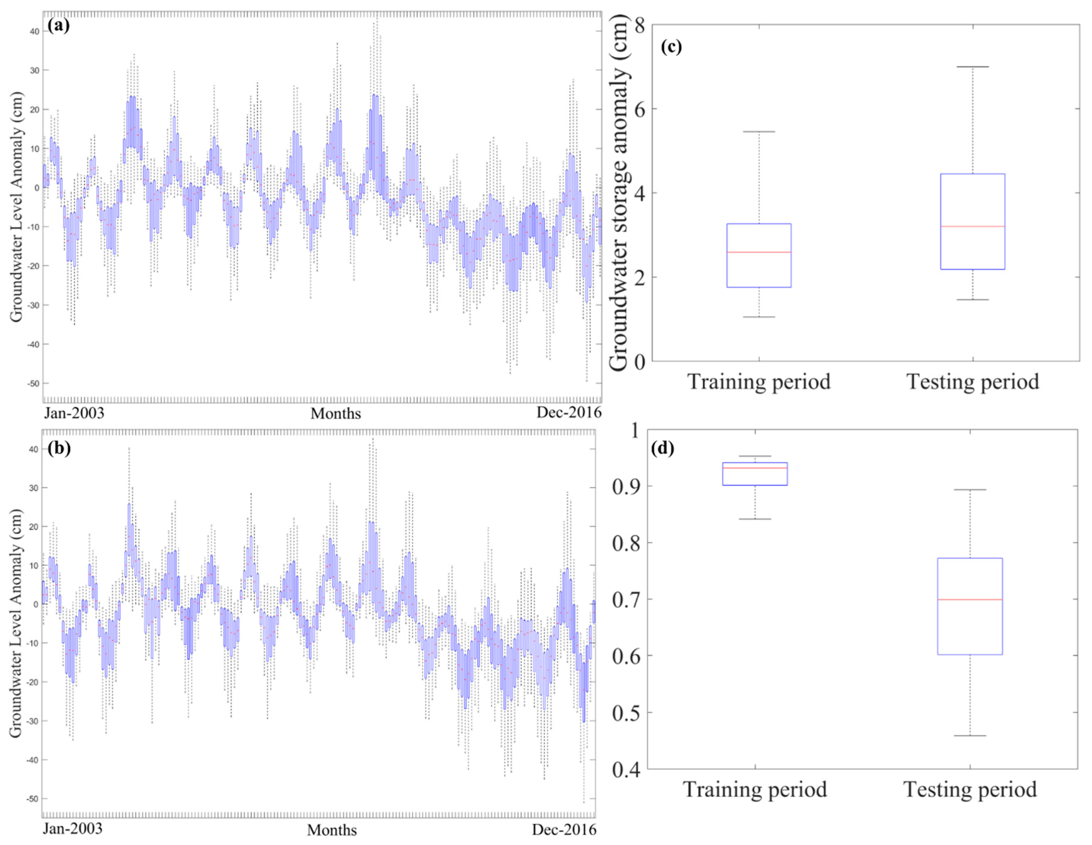
The ARIMA model was then established for each grid with the order as summarized in Figure 7. The resulting model results were promising to forecast future groundwater variability. Figure 8a shows the monthly distribution of ARIMA forecasts during the historical period of January 2003 to December 2016 while Figure 8b shows the historical records based on GRACE-derived data for the same period and within the CRB. Under detailed observation, it can be seen that there are 164 box plots in each figure representing the monthly inter-quartile range of ΔGWS variability spatially within the CRB. The whiskers on each box plots represent the corresponding 5th and 95th percentiles. While comparing Figure 8a,b, it can be observed that the corresponding box plots are similar and the monthly variations along the abscissa are also consistent. This validates the robustness of the ARIMA for simulating the GRACE-derived ΔGWS. The boxplots in Figure 8c,d summarizes the distribution of RMSE and NSE respectively during the training and testing period for CRB. The RMSE and NSE were obtained from the simulated and GRACE-derived ΔGWS data presented in Figure 8a,b. The red line within the box plots of Figure 8c,d represent the median value while the horizontal box edges represent the 25th and 75th percentile. The whiskers represent the 5th and 95th percentile. Further, the robustness of the ARIMA model is established by NSE during both training and testing period which varies between 0.5 and 1. The median NSE during the training period was observed to be greater than 0.9 and that during the testing period was approximately 0.7. This shows the model holds very good standings as suggested by [72]. As the ARIMA model showed skillful results during the historical period from January 2003 to December 2016, the model was utilized to forecast future groundwater anomaly from January 2017 to December 2019.
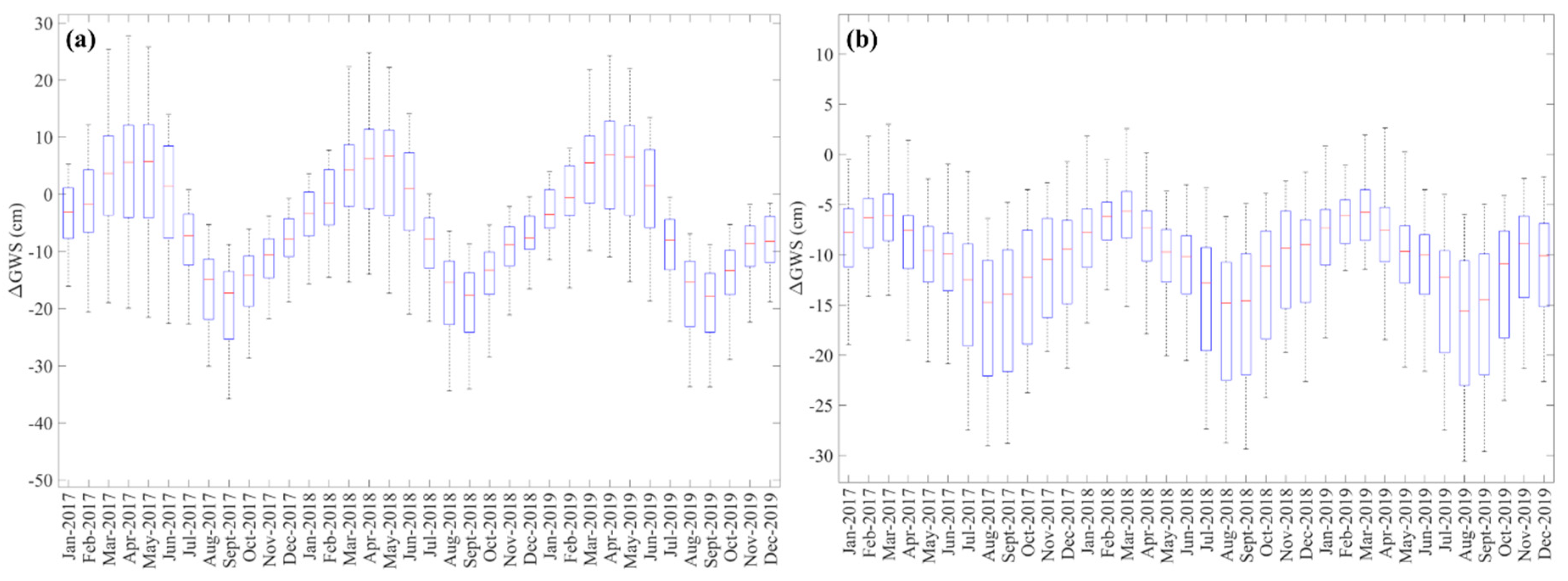
Figure 9a,b summarizes the forecasted monthly GRACE-derived ΔGWS in centimeters (cm) for upper CRB and lower CRB respectively. Each box plot shows the distribution of a monthly forecasted ΔGWS of entire grids independently for both upper and lower CRB. The boxes represent the corresponding 25th, and 75th percentile ΔGWS and the red lines represent median ΔGWS. Similarly, the whiskers represent the 5th and 95th percentiles of the corresponding ΔGWS. If the boxes lie in the positive ordinate, it shows the month will have higher groundwater storage as compared to the corresponding historical months. From Figure 9a,b, future groundwater in lower CRB is expected to decline more as compared to upper CRB as the distribution of ΔGWS is more negative for lower CRB represented by the boxes with minimal ordinates for lower CRB. It is the reflection of the ARIMA’s property of making forecasts based on the historical variations as, during the recent historical drought period, groundwater within arid and drought-affected regions CRB was withdrawn to supplement the scanty surface water. Further, the ARIMA model was able to capture the seasonality in the groundwater anomalies. From Figure 9a, it was observed ΔGWS showed positive anomaly for most of the grids in upper CRB in the months like March, April, and May as the median ΔGWS was generally positive. This can be attributed to the groundwater recharge from early snowmelts as a result of changing the climate, in the snow-covered regions of upper CRB. Most of the grids especially in lower CRB showed negative anomalies for all months. This shows the groundwater condition of the CRB is unlikely to improve in the near future as compared to the historical records. This can be attributed to higher evaporation and lower precipitation during dry seasons resulting from climate change. Further, the decline in surface water availability also causes stress on groundwater. Once the groundwater storage is declined resulting from excessive withdrawal, it causes soil consolidation reducing the recharge rate of groundwater. These factors combined hinders the improvement in groundwater conditions. As the forecasted groundwater anomalies are mostly negative during August and September, it is more likely that groundwater storage will decline during these months of near future.
6. Conclusions
The study presents the stochastic behavior of GRACE-derived groundwater time series data in CRB from January 2004 to December 2016. An ARIMA model is developed using the training data from January 2004 to December 2014 to forecast the monthly time series data from January 2015 to December 2016. A total of eleven seasonal ARIMA models with a different order of combination are tested to find the best fit model. The key findings of the current study are summarized below:
- (1)
- GRACE-derived groundwater anomaly being well correlated with in-situ groundwater data established the applicability of GRACE data in analyzing past and future groundwater analysis in the CRB.
- (2)
- The GRACE-derived change in monthly groundwater storage showed strong seasonality. Seasonal differencing was promising while making forecasts with non-stationary groundwater data.
- (3)
- The ACF and PACF plots of differencing data series were beneficial to estimate the tentative order of the ARIMA model.
- (4)
- ARIMA models order obtained based on the evaluation criteria (AIC and BIC) were found skillful. The residual analysis reinforced the idea of selection of the fitted model order.
- (5)
- ARIMA estimates of groundwater storage anomalies fit reasonably well with the observed values as supported by RMSE and NSE skills during the historical training and testing periods.
- (6)
- The ARIMA forecasts indicated the increase in March, April and May groundwater storage within the major number of grids of upper CRB. This can be attributed to the early snowmelts in the region during these months as a result of climate change.
- (7)
- The study showed a probable decline in future groundwater storage in lower CRB for all months. Additionally, the model also predicted the decline in near future groundwater storage within upper CRB for the months except for March, April, and May.
The current research will be beneficial to water resource personnel as the newly tested approach showed skillful results. The study can be tested in different regions to verify whether the model is versatile in different varieties of watershed and hydroclimate. The stochastic modeling of GRACE-derived groundwater storage anomalies can be effectively utilized for forecasting groundwater behavior. This will lead in making policies for sustainable groundwater management. Addition to forecasting the ARIMA model coupled with GRACE data can also be utilized to study past variabilities. This stochastic model can also be utilized to determine future water head and trend in CRB which will facilitate water managers to allocate the resources and resolve excessive groundwater withdrawal. Future trend analysis can also be done using the output of the fitted model. A deterministic method can reproduce the spatial scenario but shows poor performance in terms of forecasting calculation. On the other hand, a stochastic method like ARIMA, can’t replicate the spatial scenario but can predict the future trend effectively. So, the future study of incorporating ARIMA with another deterministic method can improve model performance.
Author Contributions
A.K. and S.A. designed the research idea. The results were prepared and analyzed by M.M.R. and B.T. All authors contributed towards writing the manuscript.
Funding
This research received no external funding.
Acknowledgments
The authors would like to thank the editor and two anonymous reviewers for constructive feedbacks. This research was also possible through the use of publicly available datasets, including the in- situ groundwater data in Colorado River Basin from the USGS: http://nationalmap.gov, GRACE data from http://grace.jpl.nasa.gov, and GLDAS data abstracted from https://ldas.gsfc.nasa.gov/gldas/. The authors would like to acknowledge the Office of the Vice Chancellor for Research at Southern Illinois University, Carbondale for providing the research support.
Conflicts of Interest
The authors declare no conflict of interest.
Abbreviations
| ACF | Autocorrelation Function |
| AIC | Akaike Information Criterion |
| ARIMA | Autoregressive Integrated Moving Average |
| CRB | Colorado River Basin |
| CWS | Canopy Water Storage |
| CWSA | Canopy Water Storage Anomaly |
| GLDAS | Global Land Data Assimilation System |
| GRACE | Gravity Recovery and Climate Experiment |
| GWS | Groundwater Storage |
| GWSA | Groundwater Storage Anomalies |
| MK | Mann-Kendall |
| NSE | Nash-Sutcliffe Efficiency |
| PACF | Partial Autocorrelation Function |
| SW | Surface Water |
| SWA | Surface Water Anomaly |
| SWE | Snow Water Equivalent |
| SWEA | Snow Water Equivalent Anomaly |
| TWS | Terrestrial Water Storage |
| TWSA | Terrestrial Water Storage Anomaly |
References
- Bates, B.; Kundzewicz, Z.W.; Wu, S.; Palutikof, J.P. (Eds.) Climate Change and Water; IPCC Secretariat: Geneva, Switzerland, 2008; p. 210. [Google Scholar]
- Li, F.; Feng, P.; Zhang, W.; Zhang, T. An integrated groundwater management mode based on control indexes of groundwater quantity and level. Water Resour. Manag. 2013, 27, 3273–3292. [Google Scholar] [CrossRef]
- Mirzavand, M.; Ghazavi, R. A stochastic modelling technique for groundwater level forecasting in an arid environment using time series methods. Water Resour. Manag. 2015, 29, 1315–1328. [Google Scholar] [CrossRef]
- Rohde, M.M.; Froend, R.; Howard, J. A global synthesis of managing groundwater dependent ecosystems under sustainable groundwater policy. Groundwater 2017, 55, 293–301. [Google Scholar] [CrossRef]
- Mohanty, S.; Jha, M.K.; Kumar, A.; Sudheer, K.P. Artificial neural network modeling for groundwater level forecasting in a river island of eastern India. Water Resour. Manag. 2010, 24, 1845–1865. [Google Scholar] [CrossRef]
- Chen, J.; Li, J.; Zhang, Z.; Ni, S. Long-term groundwater variations in Northwest India from satellite gravity measurements. Glob. Planet. Chang. 2014, 116, 130–138. [Google Scholar] [CrossRef] [Green Version]
- Abidin, H.Z.; Andreas, H.; Djaja, R.; Darmawan, D.; Gamal, M. Land subsidence characteristics of Jakarta between 1997 and 2005, as estimated using GPS surveys. Gps. Solutions 2008, 12, 23–32. [Google Scholar] [CrossRef]
- Phien-Wej, N.; Giao, P.; Nutalaya, P. Land subsidence in Bangkok, Thailand. Eng. Geol. 2006, 82, 187–201. [Google Scholar] [CrossRef]
- Gleeson, T.; Wada, Y.; Bierkens, M.F.; van Beek, L.P. Water balance of global aquifers revealed by groundwater footprint. Nature 2012, 488, 197. [Google Scholar] [CrossRef]
- Prinos, S.T.; Lietz, A.; Irvin, R. Design of A Real-Time Ground-Water Level Monitoring Network and Portrayal of Hydrologic Data in Southern Florida (No. 2001–4275); Geological Survey (US): Reston, WV, USA, 2002.
- Becker, M.W. Potential for satellite remote sensing of ground water. Groundwater 2006, 44, 306–318. [Google Scholar] [CrossRef]
- Chen, J.; Famigliett, J.S.; Scanlon, B.R.; Rodell, M. Groundwater storage changes: Present status from GRACE observations. Surv. Geophys. 2016, 37, 397–417. [Google Scholar] [CrossRef]
- Landerer, F.W.; Swenson, S.C. Accuracy of scaled GRACE terrestrial water storage estimates. Water Resour. Res. 2012, 48. [Google Scholar] [CrossRef] [Green Version]
- Tapley, B.D.; Bettadpur, S.; Ries, J.C.; Thompson, P.F.; Watkins, M.M. GRACE measurements of mass variability in the Earth system. Science 2004, 305, 503–505. [Google Scholar] [CrossRef]
- Iqbal, N.; Hossain, F.; Lee, H.; Akhter, G. Satellite gravimetric estimation of groundwater storage variations over Indus Basin in Pakistan. IEEE J. Sel. Top Appl. Earth Obs. Remote Sens. 2016, 9, 3524–3534. [Google Scholar] [CrossRef]
- Nanteza, J.; de Linage, C.R.; Thomas, B.F.; Famiglietti, J.S. Monitoring groundwater storage changes in complex basement aquifers: An evaluation of the GRACE satellites over East Africa. Water Resour. Res. 2016, 52, 9542–9564. [Google Scholar] [CrossRef] [Green Version]
- Pradhan, G. Understanding Interannual Groundwater Variability in North India using GRACE. Master’s Thesis, University of Twente, Enschede, The Netherlands, 2014. [Google Scholar]
- Seo, J.Y.; Lee, S.-I. Integration of GRACE, ground observation, and land-surface models for groundwater storage variations in South Korea. Int. J. Remote Sens. 2016, 37, 5786–5801. [Google Scholar] [CrossRef]
- Bhanja, S.N.; Mukherjee, A.; Saha, D.; Velicogna, I.; Famiglietti, J.S. Validation of GRACE based groundwater storage anomaly using in-situ groundwater level measurements in India. J. Hydrol. 2016, 543, 729–738. [Google Scholar] [CrossRef]
- Katpatal, Y.B.; Rishma, C.; Singh, C.K. Sensitivity of the gravity recovery and climate experiment (GRACE) to the complexity of aquifer systems for monitoring of groundwater. Hydrogeol. J. 2018, 26, 933–943. [Google Scholar] [CrossRef]
- Liesch, T.; Ohmer, M. Comparison of GRACE data and groundwater levels for the assessment of groundwater depletion in Jordan. Hydrogeol. J. 2016, 24, 1547–1563. [Google Scholar] [CrossRef]
- Muskett, R.R.; Romanovsky, V.E. Groundwater storage changes in arctic permafrost watersheds from GRACE and in situ measurements. Environ. Res. Lett. 2009, 4, 045009. [Google Scholar] [CrossRef]
- Strassberg, G.; Scanlon, B.R.; Chambers, D. Evaluation of groundwater storage monitoring with the GRACE satellite: Case study of the high plains aquifer, central United States. Water Resour. Res. 2009, 45. [Google Scholar] [CrossRef]
- Sun, A.Y. Predicting groundwater level changes using GRACE data. Water Resour. Res. 2013, 49, 5900–5912. [Google Scholar] [CrossRef] [Green Version]
- Hamed, K.H.; Rao, A.R. A modified Mann-Kendall trend test for autocorrelated data. J. Hydrol. 1998, 204, 182–196. [Google Scholar] [CrossRef]
- Kumar, S.; Merwade, V.; Kam, J.; Thurner, K. Streamflow trends in Indiana: Effects of long term persistence, precipitation and subsurface drains. J. Hydrol. 2009, 374, 171–183. [Google Scholar] [CrossRef]
- Sang, Y.F.; Wang, Z.; Liu, C. Comparison of the MK test and EMD method for trend identification in hydrological time series. J. Hydrol. 2014, 510, 293–298. [Google Scholar] [CrossRef]
- Pathak, P.; Kalra, A.; Ahmad, S. Temperature and precipitation changes in the Midwestern United States: implications for water management. Int. J. Water Resour. Dev. 2017, 33, 1003–1019. [Google Scholar] [CrossRef]
- Kendall, M. Multivariate Analysis; Charles Griffin b Co. LTD.: London, UK, 1975; p. 210. [Google Scholar]
- Mann, H.B. Nonparametric tests against trend. Econometrica 1945, 13, 245–259. [Google Scholar] [CrossRef]
- Sen, P.K. Estimates of the regression coefficient based on Kendall’s tau. J. Am. Stat. Assoc. 1968, 63, 1379–1389. [Google Scholar] [CrossRef]
- Emamgholizadeh, S.; Moslemi, K.; Karami, G. Prediction the groundwater level of bastam plain (Iran) by artificial neural network (ANN) and adaptive neuro-fuzzy inference system (ANFIS). Water Resour. Manag. 2014, 28, 5433–5446. [Google Scholar] [CrossRef]
- Daliakopoulos, I.N.; Coulibaly, P.; Tsanis, I.K. Groundwater level forecasting using artificial neural networks. J. Hydrol. 2005, 309, 229–240. [Google Scholar] [CrossRef]
- Mohanty, S.; Jha, M.K.; Kumar, A.; Sudheer, K.P. Using artificial neural network approach for simultaneous forecasting of weekly groundwater levels at multiple sites. Water Resour. Manag. 2015, 29, 5521–5532. [Google Scholar] [CrossRef]
- Nourani, V.; Nadiri, A.; Moghaddam, A.; Singh, V. Forecasting Spatiotemproal Water Levels of Tabriz Aquifer. Available online: https://oaktrust.library.tamu.edu/handle/1969.1/164642 (accessed on 17 November 2018).
- Wu, J.; Hu, B.X.; Zhang, D.; Shirley, C. A three-dimensional numerical method of moments for groundwater flow and solute transport in a nonstationary conductivity field. Adv. Water Resour. 2003, 26, 1149–1169. [Google Scholar] [CrossRef]
- Castellano-Méndez, M.; González-Manteiga, W.; Febrero-Bande, M.; Prada-Sánchez, J.M.; Lozano-Calderón, R. Modelling of the monthly and daily behaviour of the runoff of the Xallas river using Box–Jenkins and neural networks methods. J. Hydrol. 2004, 296, 38–58. [Google Scholar] [CrossRef]
- Abdullahi, M.; Toriman, M.E.; Gasim, M.B.; Garba, I. Trends analysis of groundwater: using non-parametric methods in Terengganu Malaysia. J. Earth Sci. Clim. Chang. 2015, 6, 2. [Google Scholar]
- Gibrilla, A.; Anornu, G.; Adomako, D. Trend analysis and ARIMA modelling of recent groundwater levels in the White Volta River basin of Ghana. Groundw. Sustain Dev. 2018, 6, 150–163. [Google Scholar] [CrossRef]
- Mack, T.J.; Chornack, M.P.; Taher, M.R. Groundwater-level trends and implications for sustainable water use in the Kabul Basin, Afghanistan. Environ. Sys. Decisions 2013, 33, 457–467. [Google Scholar] [CrossRef] [Green Version]
- Yang, Z.; Lu, W.; Long, Y.; Li, P. Application and comparison of two prediction models for groundwater levels: A case study in Western Jilin Province, China. J. Arid Environ. 2009, 73, 487–492. [Google Scholar] [CrossRef]
- Box, G.E.; Jenkins, G.M. Time Series Analysis: Forecasting and Control; Holden Day Inc.: San Francisco, CA, USA, 1976. [Google Scholar]
- Gharde, K.D.; Kothari, M.; Mahale, D.M. Developed seasonal ARIMA model to forecast streamflow for Savitri Basin in Konkan Region of Maharshtra on daily basis. J. Indian Soc. Coastal Agric. Res. 2016, 34, 110–119. [Google Scholar]
- Myronidis, D.; Ioannou, K.; Fotakis, D.; Dörflinger, G. Streamflow and hydrological drought trend analysis and forecasting in Cyprus. Water Resour. Manag. 2018, 32, 1759–1776. [Google Scholar] [CrossRef]
- Yu, Z.; Lei, G.; Jiang, Z.; Liu, F. ARIMA modelling and forecasting of water level in the middle reach of the Yangtze River. In Proceedings of the 4th International Conference on Transportation Information and Safety (ICTIS), Banff, Canada, 8–10 August 2017. [Google Scholar]
- Valipour, M. Long-term runoff study using SARIMA and ARIMA models in the United States. Meterol. Appl. 2015, 22, 592–598. [Google Scholar] [CrossRef] [Green Version]
- Ghimire, B.N. Application of ARIMA model for river discharges analysis. J. Nepal Phys. Soc. 2017, 4, 27–32. [Google Scholar] [CrossRef]
- Katimon, A.; Shahid, S.; Mohsenipour, M. Modeling water quality and hydrological variables using ARIMA: A case study of Johor River, Malaysia. Sustain. Water Resour. Manag. 2018, 4, 991–998. [Google Scholar] [CrossRef]
- Bin Shaari, M.A.; Samsudin, R.; Bin Shabri Ilman, A. Comparison of drought forecasting using ARIMA and empirical wavelet transform-ARIMA. In Proceedings of International Conference of Reliable Information and Communication Technology; Springe: Cham, Switzerland, 2018; pp. 449–458. [Google Scholar]
- Jerla, C.; Prairie, J.; Adams, P. Colorado River Basin Water Supply and Demand Study: Study Report. Available online: https://www.usbr.gov/lc/region/programs/crbstudy/finalreport/Study%20Report/StudyReport_FINAL_Dec2012.pdf (accessed on 3 November 2018).
- Scanlon, B.R.; Zhang, Z.; Reedy, R.C.; Pool, D.R.; Save, H.; Long, D.; Chen, J.; Wolock, D.M.; Conway, B.D.; Winester, D. Hydrologic implications of GRACE satellite data in the Colorado River Basin. Water Resour. Res. 2015, 51, 9891–9903. [Google Scholar] [CrossRef]
- Castle, S.L.; Thomas, B.F.; Reager, J.T.; Rodell, M.; Swenson, S.C.; Famiglietti, J.S. Groundwater depletion during drought threatens future water security of the Colorado River Basin. Geophys. Res. Lett. 2014, 41, 5904–5911. [Google Scholar] [CrossRef] [PubMed] [Green Version]
- Castle, S.; Thomas, B.; Reager, J.T.; Swenson, S.C.; Famiglietti, J.S. Quantifying Changes in Accessible Water in the Colorado River Basin. In Proceedings of the AGU Fall 2013 Meeting, San Francisco, CA, USA, 9–13 December 2013. [Google Scholar]
- Rodell, M.; Houser, P.; Jambor, U.; Gottschalck, J.; Mitchell, K.; Meng, C.; Arsenault, K.; Cosgrove, B.; Radakovich, J.; Bosilovich, M. The global land data assimilation system. Bull. Am. Meteorol. Soc. 2004, 85, 381–394. [Google Scholar] [CrossRef]
- Ramillien, G.; Famiglietti, J.S.; Wahr, J. Detection of continental hydrology and glaciology signals from GRACE: A review. Surv. Geophys. 2008, 29, 361–374. [Google Scholar] [CrossRef]
- Schmidt, R.; Flechtner, F.; Meyer, U.; Neumayer, K.-H.; Dahle, C.; König, R.; Kusche, J. Hydrological signals observed by the GRACE satellites. Surv. Geophys. 2008, 29, 319–334. [Google Scholar] [CrossRef]
- Swenson, S. GRACE Monthly Land Water Mass Grids NETCDF Release 5.0. Ver. 5.0. PO. DAAC, CA, USA. Available online: ftp://podaac-ftp.jpl.nasa.gov/allData/tellus/L3/land_mass/RL05/netcdf/ (accessed on 10 August 2018).
- Wiese, D. GRACE monthly global water mass grids NETCDF RELEASE 5.0. Ver. 5.0, PO. DAAC, CA, USA. 2015. Available online: https://doi. org/10.5067/TEMSC-OCL05 (accessed on 1 June 2017).
- Liu, R.; Zou, R.; Li, J.; Zhang, C.; Zhao, B.; Zhang, Y. Vertical displacements driven by groundwater storage changes in the north China plain detected by GPS observations. Remote Sens. 2018, 10, 259. [Google Scholar] [CrossRef]
- Moritz, S.; Bartz-Beielstein, T. ImputeTS: Time series missing value imputation in R. The R J. 2017, 9, 207–218. [Google Scholar] [CrossRef]
- Ediger, V.Ş.; Akar, S. ARIMA forecasting of primary energy demand by fuel in Turkey. Energy Policy 2007, 35, 1701–1708. [Google Scholar] [CrossRef]
- Sakumura, C.; Bettadpur, S.; Bruinsma, S. Ensemble prediction and intercomparison analysis of GRACE time-variable gravity field models. Geophys. Res. Lett. 2014, 41, 1389–1397. [Google Scholar] [CrossRef] [Green Version]
- Dai, Y.; Zeng, X.; Dickinson, R.E.; Baker, I.; Bonan, G.B.; Bosilovich, M.G.; Oleson, K.W. The common land model. Bull. Am. Meteorol. Soc. 2003, 84, 1013–1024. [Google Scholar] [CrossRef]
- Liang, X.; Lettenmaier, D.P.; Wood, E.F.; Burges, S.J. A simple hydrologically based model of land surface water and energy fluxes for general circulation models. J. Geophys. Res. Atmos. 1994, 99, 14415–14428. [Google Scholar] [CrossRef]
- Ek, M.B.; Mitchell, K.E.; Lin, Y.; Rogers, E.; Grunmann, P.; Koren, V.; Tarpley, J.D. Implementation of Noah land surface model advances in the National Centers for Environmental Prediction operational mesoscale Eta model. J. Geophys. Res. Atmos. 2003, 108. [Google Scholar] [CrossRef] [Green Version]
- Koster, R.D.; Suarez, M.J. Energy and water balance calculations in the Mosaic LSM. NOAA, Goddard Space Flight Center, Laboratory for Atmospheres, Data Assimilation Office: Laboratory for Hydrospheric Processes. Available online: https://gmao.gsfc.nasa.gov/pubs/docs/Koster130.pdf (accessed on 5 October 2018).
- Akaike, H. A new look at the statistical model identification. IEEE Trans. Automat. Contr. 1974, 19, 716–723. [Google Scholar] [CrossRef]
- Bowerman, B.; O’Connell, R. Forecasting and Time Series: An Applied Approach; Duxbury Press: Belmont, CA, USA, 1993. [Google Scholar]
- Sullivan, A.; White, D.D.; Hanemann, M. Designing collaborative governance: Insights from the drought contingency planning process for the lower Colorado River basin. Environ. Sci. Policy 2019, 91, 39–49. [Google Scholar] [CrossRef]
- Hyndman, R.J.; Athanasopoulos, G. Forecasting: Principles and Practice; Otexts: Melbourne, Australia, 2013. [Google Scholar]
- Tillman, F.D.; Gangopadhyay, S.; Pruitt, T. Changes in groundwater recharge under projected climate in the upper Colorado River basin. Geophys. Res. Lett. 2016, 43, 6968–6974. [Google Scholar] [CrossRef]
- Moriasi, D.N.; Arnold, J.G.; Van Liew, B.M.W.; Harmel, R.D.; Veith, T.L. Model evaluation guidelines for systematic quantification of accuracy in watershed simulations. Trans. ASABE 2006, 50, 885–900. [Google Scholar] [CrossRef]
Figure 1.
Study area showing the Upper and Lower Colorado River Basin. The grids represent the spatial resolution (1° × 1°) of the utilized GRACE data.
Figure 1.
Study area showing the Upper and Lower Colorado River Basin. The grids represent the spatial resolution (1° × 1°) of the utilized GRACE data.

Figure 2.
Autoregressive Integrated Moving Average (ARIMA) modeling framework to forecast groundwater anomaly. AIC: Akaike Information Criterion; BIC: Bayesian Information Criterion; ACF: autocorrelation function.
Figure 2.
Autoregressive Integrated Moving Average (ARIMA) modeling framework to forecast groundwater anomaly. AIC: Akaike Information Criterion; BIC: Bayesian Information Criterion; ACF: autocorrelation function.

Figure 3.
Average monthly time series of each hydrological component for the period of January 2003–December 2016 for (a) Upper Colorado River Basin and (b) Lower Colorado River Basin; (c) Spatial variation of Thiel Sen Slope at the significance level of p ≤ 0.05. The significance of the trend was obtained with the Mann-Kendal test.

Figure 4.
(a) Sample ACF (b) partial autocorrelation function (PACF) of Gravity Recovery and Climate Experiment (GRACE)-derived ΔGWS (groundwater storage) data for an arbitrary grid and (c) Sample seasonally differenced GRACE-derived ΔGWS data for the sample grid.
Figure 4.
(a) Sample ACF (b) partial autocorrelation function (PACF) of Gravity Recovery and Climate Experiment (GRACE)-derived ΔGWS (groundwater storage) data for an arbitrary grid and (c) Sample seasonally differenced GRACE-derived ΔGWS data for the sample grid.

Figure 5.
(a) Sample ACF of seasonally differenced GRACE-derived ΔGWS data; (b) PACF of seasonally differenced GRACE-derived ΔGWS data; (c) Sample ACF of residuals ARIMA (1,0,1) (1,1,1)12 and (d) PACF of residuals ARIMA (1,0,1) (1,1,1)12 for the sample grid.
Figure 5.
(a) Sample ACF of seasonally differenced GRACE-derived ΔGWS data; (b) PACF of seasonally differenced GRACE-derived ΔGWS data; (c) Sample ACF of residuals ARIMA (1,0,1) (1,1,1)12 and (d) PACF of residuals ARIMA (1,0,1) (1,1,1)12 for the sample grid.

Figure 6.
GRACE-derived ΔGWS and ARIMA resulted with the best fit model values and forecasted ΔGWS.

Figure 7.
ARIMA model order for each grid cells representing (a) autoregressive term (b) differencing term and (c) moving average term for both (i) non-seasonal and (ii) seasonal component for the Colorado River Basin.
Figure 7.
ARIMA model order for each grid cells representing (a) autoregressive term (b) differencing term and (c) moving average term for both (i) non-seasonal and (ii) seasonal component for the Colorado River Basin.

Figure 8.
Boxplots summarizing (a) ARIMA simulated groundwater anomaly during the historical period (January, 2003–December, 2016) (b) GRACE-derived groundwater anomaly during historical period (c) distribution of RMSE and (d) NSE during training (January, 2003–December, 2014) and testing period (January, 2015–December, 2016) for all grids within the Colorado River basin.

Figure 9.
Box plot of the forecasted monthly groundwater anomalies of (a) Upper Colorado River basin and (b) Lower Colorado River basin.
Figure 9.
Box plot of the forecasted monthly groundwater anomalies of (a) Upper Colorado River basin and (b) Lower Colorado River basin.


Table 1.
AIC and BIC values for different models.
| Model | AIC | BIC |
|---|---|---|
| ARIMA (1,0,1) (1,1,0)12 | 321.65 | 332.23 |
| ARIMA (1,0,1) (1,1,1)12 | 311.13 | 324.25 |
| ARIMA (0,0,1) (0,1,1)12 | 452.36 | 460.35 |
| ARIMA (0,0,1) (0,1,0)12 | 459.58 | 464.95 |
| ARIMA (0,0,2) (0,1,0)12 | 352.74 | 365.87 |
| ARIMA (1,0,2) (1,1,0)12 | 322.2 | 335.32 |
| ARIMA (2,0,1) (1,1,0)12 | 312.43 | 328.07 |
| ARIMA (2,0,1) (1,1,1)12 | 315.28 | 330.91 |
| ARIMA (1,0,2) (2,1,0) 12 | 313.82 | 329.45 |
| ARIMA (1,0,2) (1,1,1)12 | 311.86 | 327.49 |
| ARIMA (2,0,2) (2,1,2)12 | 317.13 | 340.03 |
© 2019 by the authors. Licensee MDPI, Basel, Switzerland. This article is an open access article distributed under the terms and conditions of the Creative Commons Attribution (CC BY) license (http://creativecommons.org/licenses/by/4.0/).
Share and Cite
MDPI and ACS Style
Rahaman, M.M.; Thakur, B.; Kalra, A.; Ahmad, S. Modeling of GRACE-Derived Groundwater Information in the Colorado River Basin. Hydrology 2019, 6, 19. https://doi.org/10.3390/hydrology6010019
AMA Style
Rahaman MM, Thakur B, Kalra A, Ahmad S. Modeling of GRACE-Derived Groundwater Information in the Colorado River Basin. Hydrology. 2019; 6(1):19. https://doi.org/10.3390/hydrology6010019
Chicago/Turabian StyleRahaman, Md Mafuzur, Balbhadra Thakur, Ajay Kalra, and Sajjad Ahmad. 2019. "Modeling of GRACE-Derived Groundwater Information in the Colorado River Basin" Hydrology 6, no. 1: 19. https://doi.org/10.3390/hydrology6010019
Note that from the first issue of 2016, this journal uses article numbers instead of page numbers. See further details here.