A Remote Sensing Approach to Environmental Monitoring in a Reclaimed Mine Area


1
NOVA IMS, Universidade Nova de Lisboa, Campus de Campolide, 1070-312 Lisbon, Portugal
2
Stockholm Resilience Centre, Stockholm University, Kraftriket 2B, SE-106 91 Stockholm, Sweden
*
Author to whom correspondence should be addressed.
ISPRS Int. J. Geo-Inf. 2017, 6(12), 401; https://doi.org/10.3390/ijgi6120401
Submission received: 1 November 2017
/
Revised: 6 December 2017
/
Accepted: 8 December 2017
/
Published: 10 December 2017
Abstract
:Mining for resources extraction may lead to geological and associated environmental changes due to ground movements, collision with mining cavities, and deformation of aquifers. Geological changes may continue in a reclaimed mine area, and the deformed aquifers may entail a breakdown of substrates and an increase in ground water tables, which may cause surface area inundation. Consequently, a reclaimed mine area may experience surface area collapse, i.e., subsidence, and degradation of vegetation productivity. Thus, monitoring short-term landscape dynamics in a reclaimed mine area may provide important information on the long-term geological and environmental impacts of mining activities. We studied landscape dynamics in Kirchheller Heide, Germany, which experienced extensive soil movement due to longwall mining without stowing, using Landsat imageries between 2013 and 2016. A Random Forest image classification technique was applied to analyze land-use and landcover dynamics, and the growth of wetland areas was assessed using a Spectral Mixture Analysis (SMA). We also analyzed the changes in vegetation productivity using a Normalized Difference Vegetation Index (NDVI). We observed a 19.9% growth of wetland area within four years, with 87.2% growth in the coverage of two major waterbodies in the reclaimed mine area. NDVI values indicate that the productivity of 66.5% of vegetation of the Kirchheller Heide was degraded due to changes in ground water tables and surface flooding. Our results inform environmental management and mining reclamation authorities about the subsidence spots and priority mitigation areas from land surface and vegetation degradation in Kirchheller Heide.
1. Introduction
Mining is an important source of raw materials and minerals, e.g., metals, salt, and coal, for industrial and domestic usage [1,2]. Countries in the European Union (EU) produce about 7% of the industrial and domestic commodities from mine-extracted resources [2]. Mining industries also play a vital role in global to regional economies, e.g., in energy production and fuel supply [1].
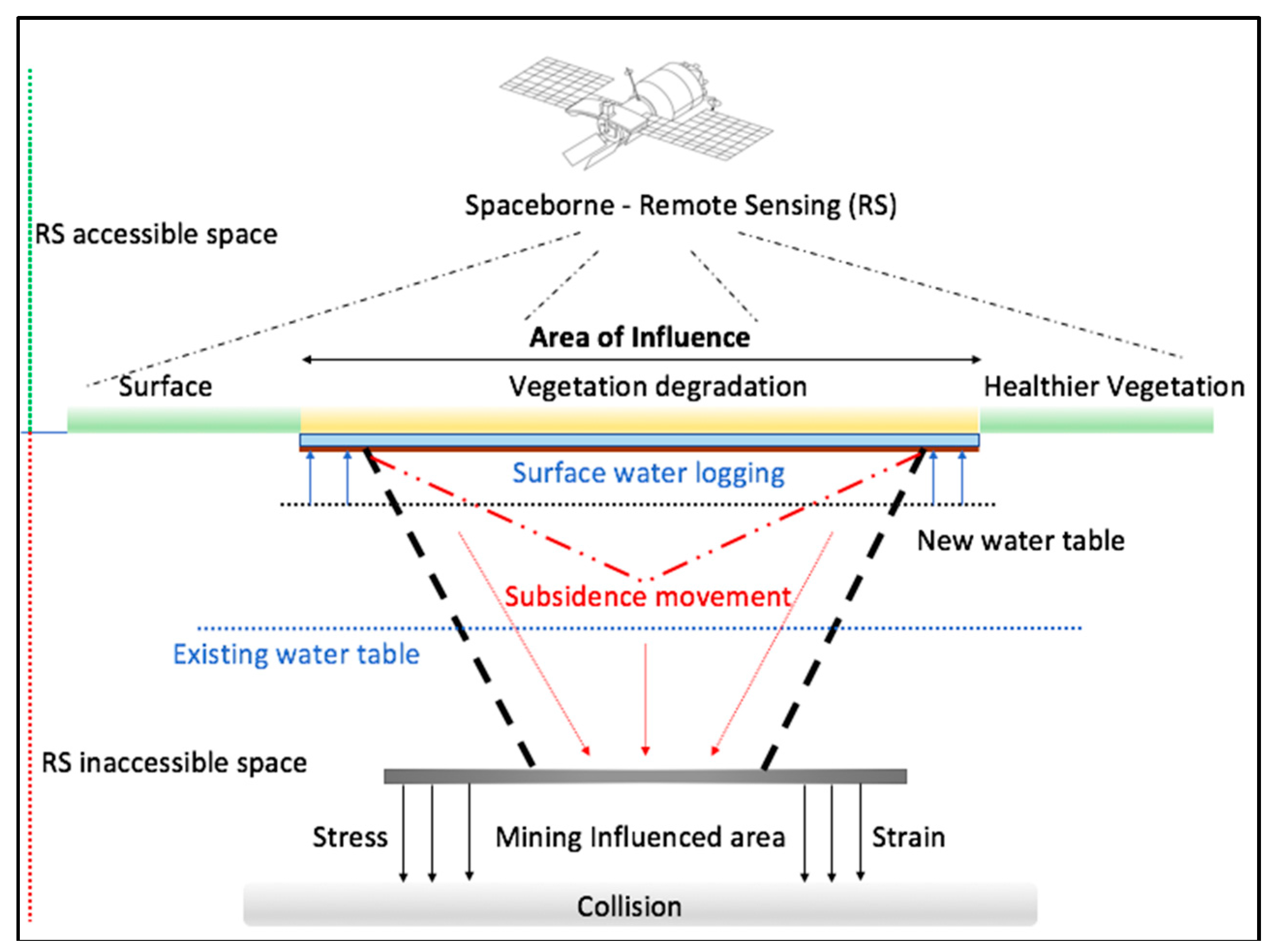
Mining activities may lead to several geological changes, i.e., ground movements, collision with mining cavities, and deformation of aquifers (Figure 1). These changes may constitute an increase in the groundwater table, and thus a slow sinking of subsurface soils and an unexpected collapse, i.e., subsidence [2]. The extraction processes and machines used to access mine galleries may produce irreversible damage in soil cohesion and eventually compress soil substrates [3,4]. Consequently, groundwater may intrude the surface level, form new waterbodies, and cause inundation. This, in turn, leads to several adverse long-term environmental impacts, such as vegetation degradation, soil erosion, flooding, sinkhole formation, and soil and water contamination [5,6,7,8], as well as to the damage of infrastructures [8,9]. The geological changes and associated environmental impacts may continue even after reclamations, if mines are not properly backfilled [10,11,12].
Regular landscape management and monitoring at the surface level are crucial for the prevention of subsidence and development of early warning systems in a reclaimed mine area (Figure 1). These are also vital for environmental protection, as well as for mitigation of the aftermaths from mining activities [8]. Particularly, monitoring short-term landscape dynamics, i.e., changes in the extent of waterbodies and vegetation, may provide important information about long-term geological changes such as subsidence, sinkhole formation, and changes in water table dynamics and associated effects on the environment [9]. In addition, changes in the productivity of vegetation is an important indicator for assessing the geological changes in an active and reclaimed mine area [13,14]. Productivity of vegetation may surrogate ecological health as well as growth of water bodies and plant stress [8].
Remote Sensing (RS) techniques and Geographic Information Systems (GIS) have shown clear advantages over conventional field monitoring and laboratory measurements for assessing long- to short-term landscape dynamics [15,16,17]. Particularly for large areas, where surveying using Global Positioning System (GPS) and ground levelling are time-consuming, expensive, and labor-intensive, RS and GIS provide prompt and efficient information on geological changes and subsidence [4]. These techniques are also useful for detecting changes in vegetation productivity and cover and flood dynamics through land-use and landcover maps [17,18]. Multispectral satellite images allow for detecting gradual as well as abrupt changes in landscapes [19]. However, besides widespread application in monitoring general landscape dynamics, the application of RS and GIS in monitoring and assessing mining effects on landscapes and environment and in associated geological changes and vegetation productivity dynamics is limited [10,11,12,13,14,20]. Although high-resolution Light Amplification by Stimulated Emission of Radiation (LASER), Interferometric Synthetic Aperture Radar (InSAR), and Light Detection and Ranging (LIDAR) mapping have been sparsely applied in small areas, environmental impacts in large mine reclamation areas have rarely been investigated using RS and GIS techniques [21,22,23,24,25,26,27].
This study aims to identify the subsidence zones and vegetation productivity degradation in a reclaimed mine area through the analyses of short-term landscape dynamics using RS and GIS techniques. The specific objectives were:
- (1)
- To examine the short-term, i.e., during 4 years, land-use and landcover (LULC) dynamics in the reclaimed mine area;
- (2)
- To quantify the emergence and growth of wetlands in the mining-influenced area and thus identify potential subsidence spots, i.e., spots exhibiting abrupt growth of waterbodies; and
- (3)
- To examine the vegetation productivity dynamics as a surrogate of the ground water table fluctuation and ecological stress.
2. Study Area
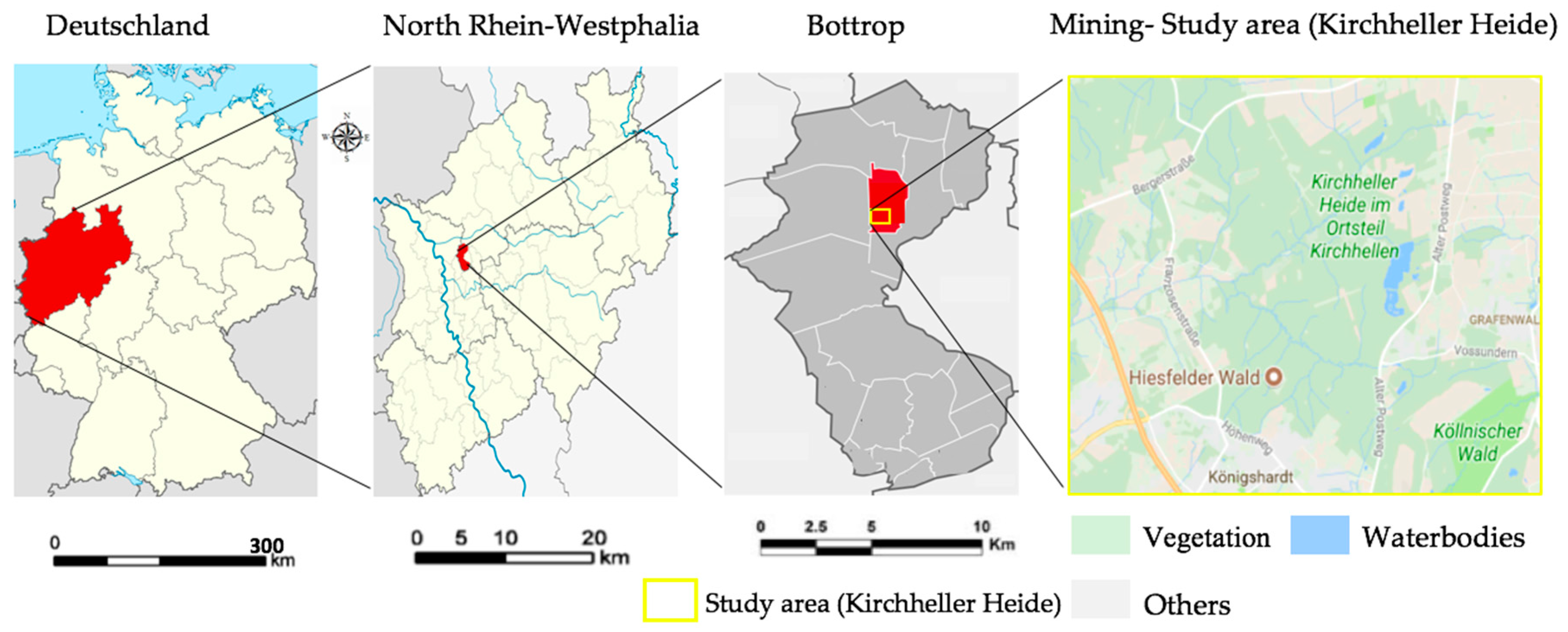
The study area, “Kirchheller Heide” (in English “Kirchhellen Heath”), is located in western Germany, surrounded by the towns of Bottrop and Huxe in the North, Oberhausen in the South, Gladbeck in the East, and Dinslanken in the West (Figure 2). The mining reclamation area lies between 51°34′53′′ N and 6°51′50′′ E and covers an area of about 57.74 km2. This site is one of the recreation areas for 7.5 million residents of the Kirchheller Heide and Ruhr district [2,8].
The area was a major industrial region dominated by 229 coal and steel mines from the second half of the 19th to the end of the 20th century, which produced approximately 400,000 tons of coal per year [2,8]. The coal was extracted from this area from depths up to 1500 m using the longwall mining method [2]. This mining method creates cavities in the ground and rock formation, which may result in surface subsidence and changes in the ground water table [20]. Moreover, 88.9% of production area was not properly backfilled when it was reclaimed during the 1990s [1,8]. Improper backfilling often leads to surface and sub-surface level depressions, while the magnitude of depressions depends on the length of long walls and the dip and width of the mined area [1,2,3,4,8]. Usually, such depressions and surface movements start six months after reclamation and gradually result into subsidence, surface area inundation, and vegetation degradation [3]. Hence, Kirchheller Heide was chosen to study potential occurrence of subsidence, inundation, and vegetation degradation caused by mining activities [8].
GMES4Mining team and EU-project MINEO have monitored the wetland and vegetation dynamics in Kircheller Heide until 2012 [1,2,3,8]. These monitoring programs have detected incidences and passive impacts of surface flooding and subsidence using ground monitoring and air-borne hyperspectral images [3]. However, this monitoring was tedious, lengthy, and stopped after October 2012, largely because hyperspectral sensors could not cover the area in a continuous mode, i.e., mono-temporal, and hence, continuous monitoring was impossible [8,28,29,30,31]. Consequently, we aim to quantify landscape dynamics as well as to identify potential subsidence zones and vegetation degradation in Kircheller Heide after 2012, i.e., during 2013–2016, using imageries from sensors that continuously captured images of the area at a regular (yearly) interval, i.e., Landsat ETM+.
3. Materials and Methods
3.1. Satellite Data
We used four Landsat Enhanced Thematic Mapper plus (ETM+) imageries covering the dates of 22 July 2013, 25 July 2014, 03 July 2015, and 30 July 2016, with 30 m spatial resolution. The imageries covering four years were chosen to study short-term landscape dynamics. To be consistent with seasonal variations and the vegetation productivity analysis, we selected images covering the frost-free growing season of Germany. This season starts in May (Spring) and ends in September (Fall/Autumn) [4,8]. To be further consistent with vegetation proportion, we selected images of July (growing season), which recorded consistent precipitation level varying between 28.2 and 34.4 L per m2 during 2013–2016 [32]. Landsat ETM+ data were freely downloaded from the United States Geological Survey (USGS) gateway [33].
3.2. Image Processing
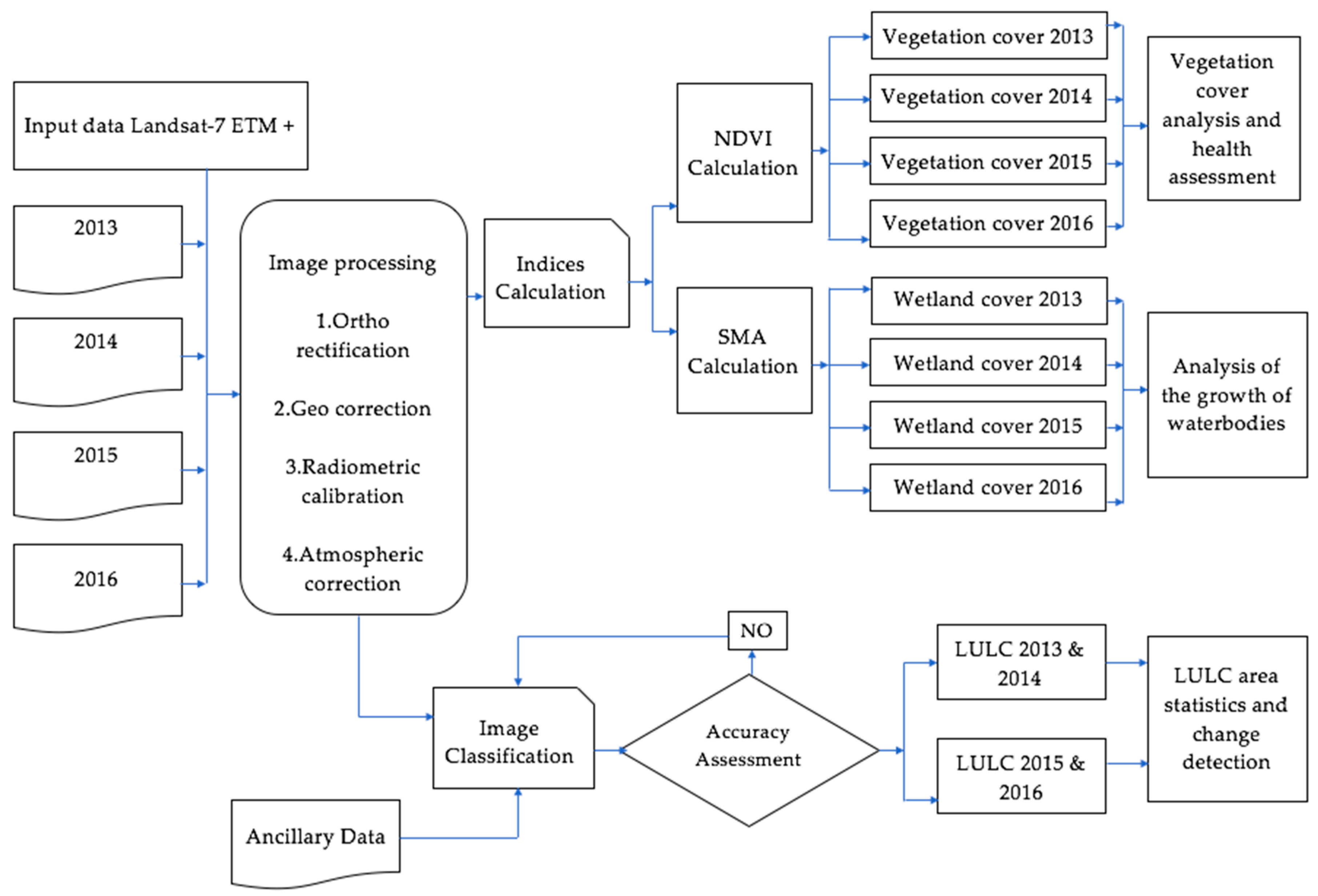
We followed a four-step procedure for investigating the landscape dynamics and vegetation productivity in Kirchheller Heide (see Figure 3). First, the satellite images were ortho-rectified and geo-corrected using the available “geoshift” and “georef” functions of the “Landsat” package in R studio [34,35,36]. Then, we geo-referenced the images using Universal Transverse Mercator (UTM) coordinate system [37]. The ETM+ images were cropped to the study area using a 10 km buffer around the mining area. To enhance the separability of the mining area from other land-use and landcover types, we applied the Tasseled Cap transformation for each imagery based on digital numbers (DN) [37].
We were cautious about the scan line error that occurred in the Landsat 7 ETM+ sensor in 2003 and subsequently affected the produced imageries in 2003 and following years [35]. To fill the data-gap, i.e., Not Available (NA) values, in the imageries that occurred due to this scan line error, we applied Landsat 7 Scan Line Corrector (SLC)-off Gap function [35]. The SLC-off images were further rectified by mosaicking as suggested by USGS [35], and the residual gaps were filled using histogram correction [38,39,40]. Scan line error correction was performed in ERDAS Imagine (version 8.7) [37].
We first distributed and stored the Landsat images in a common radiometric scale to detect and quantify changes in the landscape of Kirchheller Heide, particularly for waterbodies and vegetation. For this purpose, we converted digital number (DN) integer values (0–255) to at-satellite radiance values using the available parameters in the ETM+ metadata (radiometric calibration), i.e., Top-of-Atmosphere (TOA) radiance [39]. We also applied atmospheric correction to overcome the mismatch between surface reflectance and at-sensor reflectance. The cloud, snow, aerosol, and cirrus were first identified and classified, and then were removed using absolute atmospheric correction, i.e., Dark Object and Modified Dark Object Subtraction Method. To ensure the homogeneity of reflectance values for the analysis of vegetation dynamics, invariant features in images across 2013–2016 were identified using the Pseudo-invariant features (PIF) function and subsequently corrected using a major axis regression. The radiometric and atmospheric corrections were conducted employing an atmospheric simulation model available in Landsat and RStool packages available in the R library [41,42,43,44,45].
3.3. Land-Use and Landcover Classification and Accuracy Assessment
We analyzed the overall surface level landscape dynamics over the four years using an unsupervised image classification technique. The images were classified for 2013, 2014, 2015, and 2016 into five land-use and landcover (LULC) classes (Table 1). We applied a Random Forest (RF) classification technique that optimizes the proximities among data points [46,47]. The RF classification algorithm constitutes the following steps:
- Draw n-tree bootstrap model from the satellite imageries;
- For each bootstrap model: grow unpruned classification according to the DN values;
- Generate N number of polygons according to the DN values;
- Choose five classification land-use classes;
- Display land-use classification.
The LULC classification was performed in R [41] using Classes and Methods for Spatial Data (Sp), Raster Geospatial Data Abstraction Library (Rgdal), Raster, and Random forests packages [44,45,46,47].
The accuracy of image classification was evaluated by comparing the classified LULC maps with reference Google Earth images from 2013 to 2016 of the study area obtained from Google Earth Engine (GEE) platform [48]. We produced a set of 75 random points and extracted those values for four different study periods. Then, the selected random point values were identified from GEE and compared to the LULC maps. We used the kappa coefficient to quantify the accuracy of the classified images using ERDAS Imagine (version 8.7) [49]. The user and producer accuracies were also calculated through a confusion matrix [19]. A kappa coefficient of more than 0.8 indicates a satisfactory accuracy of classified images, i.e., classified images are analogous to the reference data [50,51,52,53,54].
3.4. Wetland Coverage and Surface Flooding
The dynamics of wetland coverage as well as the extent of surface flooding were assessed to identify potential subsidence zones. We applied a SMA on the Landsat imageries to track the changes in wetland coverage and identify the emergence of waterbodies [55]. SMA delivers pixel estimates for water extent delineated from other landcover pixels based on available radiometric data in imageries [55] (Equations (1) and (2)). Hence, the RF classification was expanded to the SMA for an accurate and precise examination of wetland dynamics, delineated from other LULC classes.
where, DNi is the measured value of a mixed pixel in band i; DNj is the measured value of each endmember (wetland pixel); Fj is the fraction of each endmember; and r is the root mean square (rms) residual that accounts for the difference between the observed and modeled values [51]. Thus, waterbodies and their extent were delineated from other landcover classes for each year during 2013–2016. We calculated the total and individual area coverage of waterbodies in each year, as well as identified if any waterbody emerged. SMA calculation and changes in waterbodies were analyzed using R packages SP, Rgdal, Raster, and Raster Time Series Analysis (rts) [45,46,47].
3.5. Vegetation Productivity and Coverage
We calculated the Normalized Difference Vegetation Index (NDVI) for the quantification of vegetation productivity during 2013–2016 using Equation (3) [56]:
where, NIR = Near Infrared Band value and R = Red Band value recorded by the Landsat ETM+ imageries [57]. Photosynthesis is the main function of plants, which is directly associated with electromagnetic energy [58,59,60]. The spectrum of visible region strongly absorbed by green vegetation and reflects in the NIR region [61,62,63]. NDVI performed the NIR and R band-ratio to describe the relative density of vegetation greenness. Thus, we integrated plant ecological functions with available radiometric data of mining area associated with the principles of electromagnetic spectrum.
We classified the obtained NDVI values into 10 raster zones based on natural breaks to distinguish among different stages of vegetation productivity and coverage, i.e., value ranges 0.42–1, 0.08–0.42, and −1–0.08 indicated high productivity (dense canopies), medium productivity, and low productivity (mostly bare land and water) vegetation, respectively. We calculated the changes in the area coverage of each raster zone during 2013–2016 and thus quantified the dynamics in vegetation productivity and coverage. NDVI calculation and changes in vegetation productivity were analyzed using R packages SP, Rgdal, Raster, and rts [46,47].
4. Results and Discussion
4.1. Landscape Dynamics in Kirchheller Heide during 2013–2016
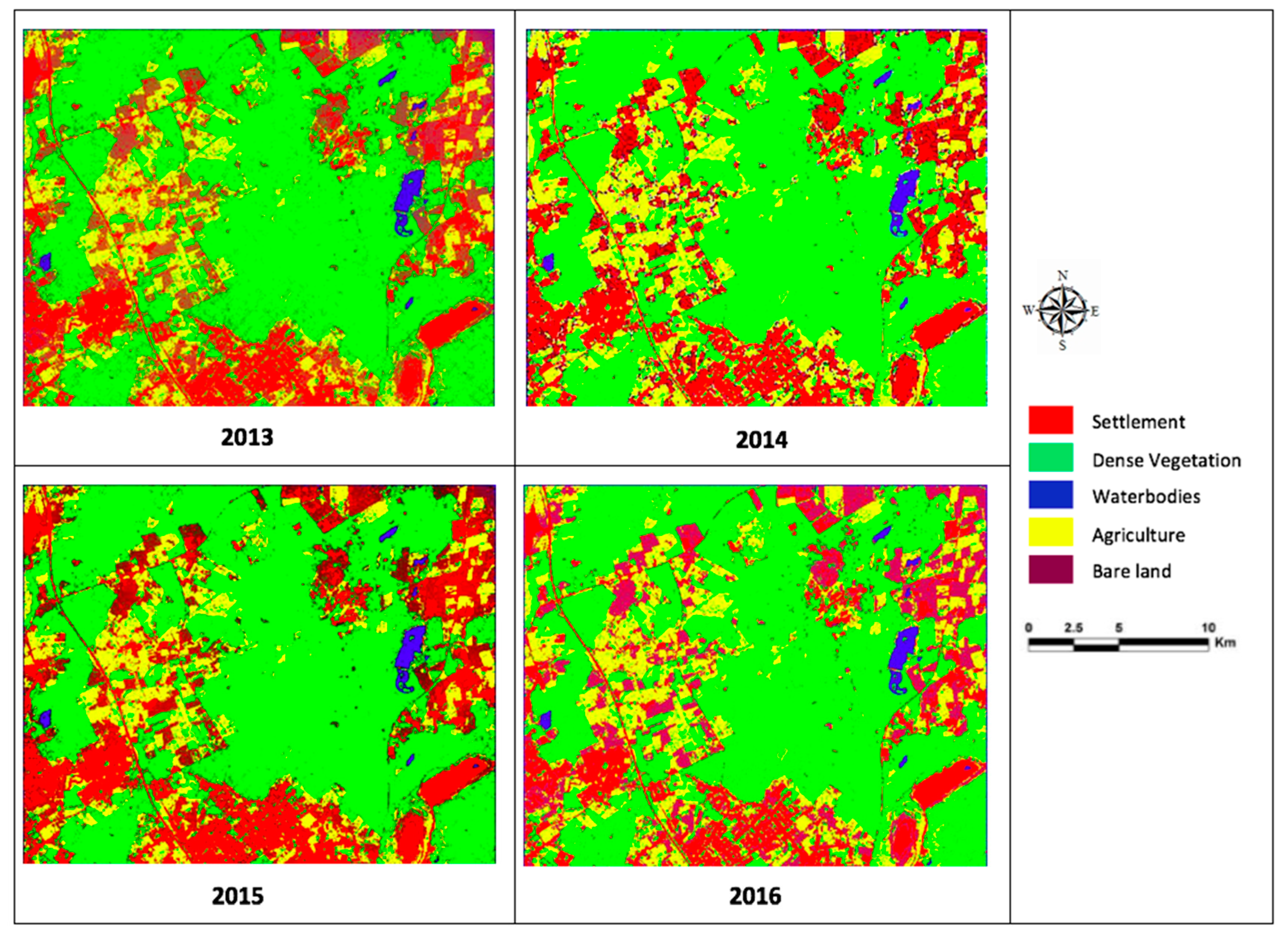
Figure 4 displays the LULC maps of Kirchheller Heide mining area obtained for July 2013, 2014, 2015, and 2016 using RF classification in R. We obtained an overall accuracy value of more than 85% for the classified LULC maps of all years with kappa coefficient values of more than 0.84 (Table 2). These values indicate a satisfactory accuracy of the classified LULC maps.
The classified LULC maps exhibit a 19.9% increase in the coverage of waterbodies between 2013 and 2016 with an annual growth rate of 6.5% (Table 3, Figure 4). This increase in the coverage of waterbodies was associated with a 5.43% decrease in the coverage of dense vegetation and 25.6% increase in the bare land area (Table 3, Figure 4). The coverage of agricultural land also exhibited a 3.2% decrease, whereas the settlement coverage increased by 5.45%. The increase in the coverage of waterbodies may relate to the subsidence and changes in ground water table in the surface level [2,3]. This subsidence may have led to collision with non-stowed mining cavities, groundwater intrusion, and caused surface flooding, which, in turn, affected and caused the decrease in the coverage of dense vegetation and agricultural lands. These results are in line with [1], which showed the relation between surface landscape dynamics and subsurface geological changes. The observed increase in the coverage of bare land may also indicate the vegetation damage caused by the subsidence and surface flooding [3,4].
4.2. Emergence and Growth of Waterbodies
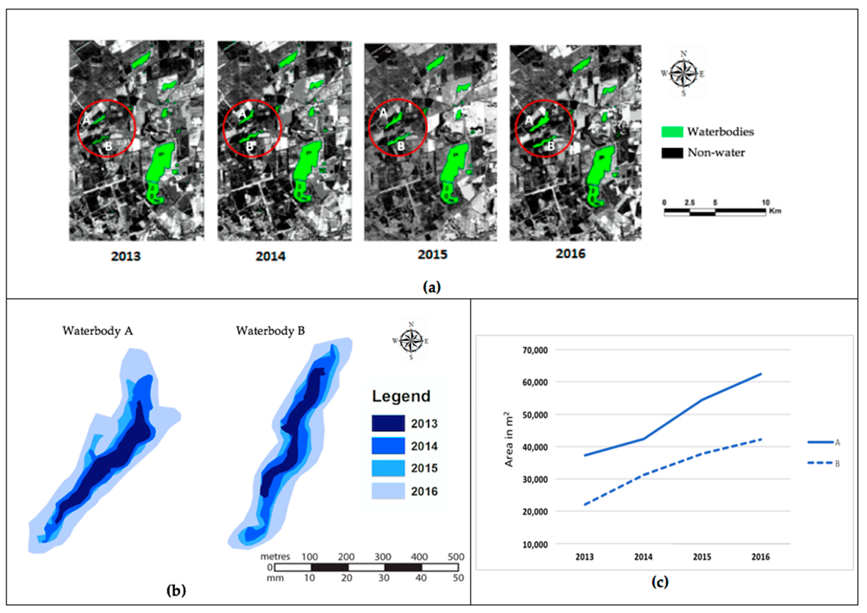
The SMA did not identify any emergence of waterbodies in Kirchheller Heide during 2013–2016 (Figure 5a). However, we observed an abrupt growth (0.06 km2) in the coverage of two waterbodies within the four years (Figure 5a). The increase in the coverage of these two waterbodies (waterbodies A and B) accounted for 87.2% of the total growth the coverage of waterbodies in Kirchheller Heide, with an annual growth rate of 29% (Figure 5b,c). Waterbodies A and B exhibited a 67% and 90% growth, respectively, in their coverage during 2013–2016 (Figure 5c). Hence, the locations of waterbodies A and B may have been the potential subsidence spots that led to surface sink, collapse, and groundwater intrusion, entailing an increase in the coverage of those waterbodies [2,3].
4.3. Vegetation Productivity
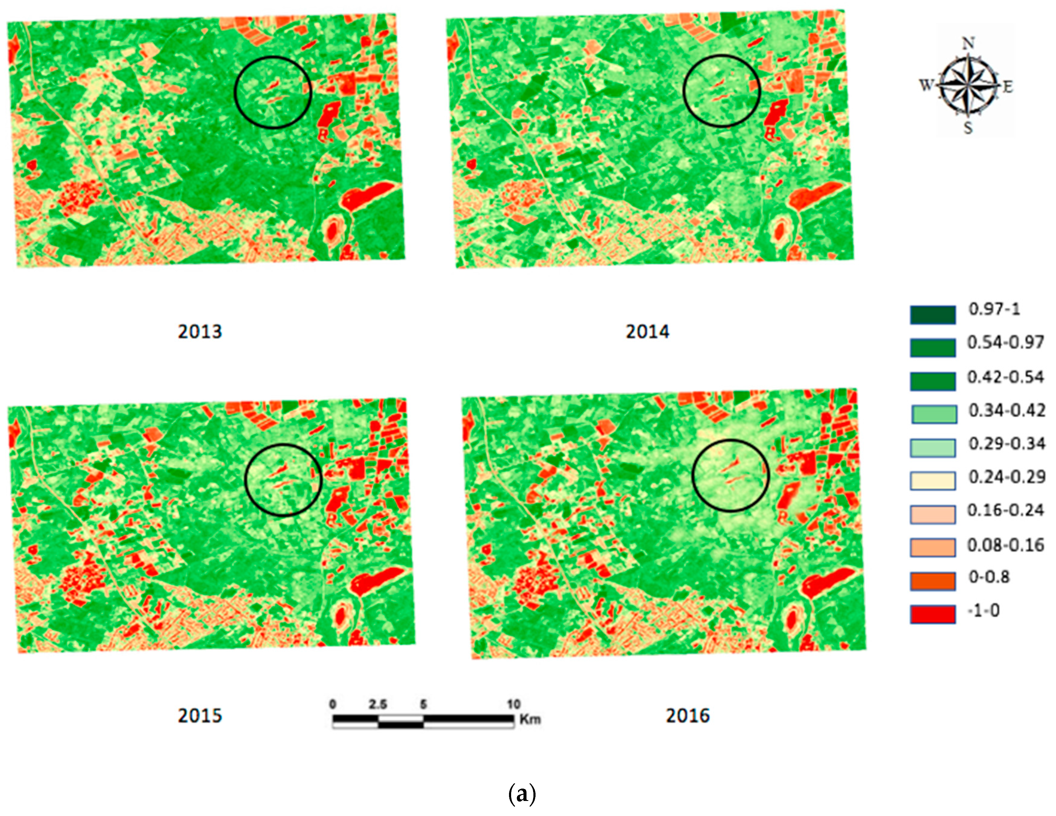
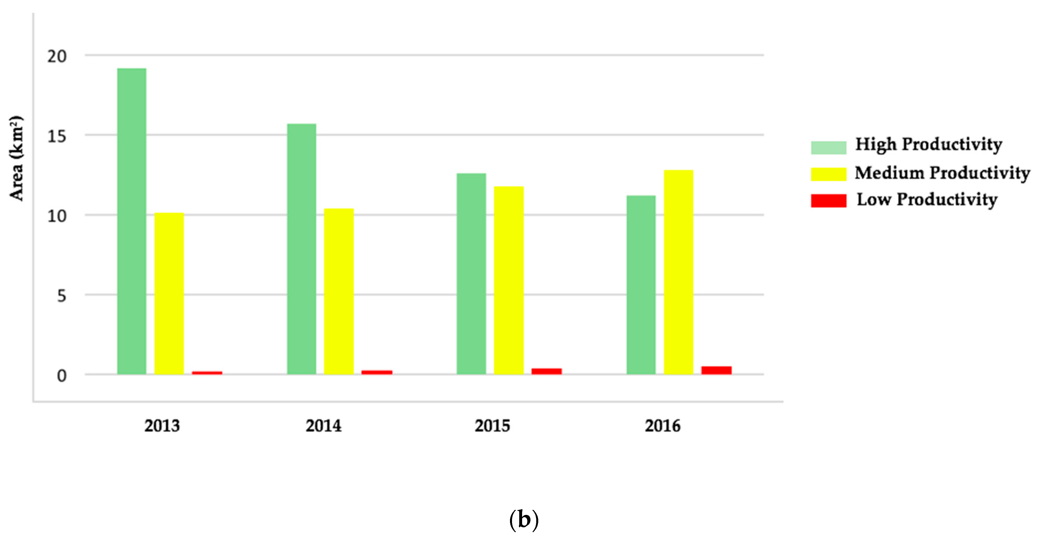
We observed a substantial decrease in the area coverage of highly productive vegetation, which was associated with an increase in the area coverage of medium and lowly productive vegetation (Figure 6, Table 4). The area around the waterbodies, which experienced the abrupt growth, was with the highest decrease in NDVI values between 2013 and 2016, i.e., the average NDVI values decreased from 0.61 to 0.29 (Figure 6). A total of 58.5% degradation in the productive vegetation mostly occurred in the neighborhood of waterbodies and along the water courses in the east (Figure 6, Table 4). Overall, the total area coverage under highly productive vegetation decreased from 56.5% to 28.3% with an annual rate of −9.5%, whereas the area coverage under medium and lowly productive vegetation increased from 14% to 76% with an annual rate of 15.5% between 2013 and 2016 (Table 4).
Our results indicate an overall degradation of vegetation productivity with substantial loss of vegetation productivity along the water course in the east of Kirchheller Heide (Figure 6, Table 4). This degradation of productivity was likely entailed by the increase in the groundwater table and consequent intrusion into the surface level (Figure 6) [3].
The variation in vegetation productivity can also be caused by confounding ecological variables, e.g., phenological characteristics (differences between growing characteristics across years). However, we controlled for the dominant drivers of seasonal variations, i.e., chose images from frost-free growing season in Germany, and precipitation level, i.e., between 28.2 and 34.4 L per m2 in July during 2013–2016, while selecting the imageries [32]. Moreover, ours is a short-term study and hence, excludes variation in plant phenological characteristics, which is usually long-term and gradual. Furthermore, the major decrease in vegetation productivity was observed for the area neighboring the waterbodies that experienced the abrupt growth. Consequently, we argue that the increase in the groundwater table caused by the subsidence is the dominant cause for the degradation of vegetation productivity in Kirchheller Heide. Increasing groundwater table led to surface flooding as well as to soil erosion, which directly influenced the vegetation productivity, as observed in the extent of NDVI values (Figure 6) [1,2].
5. Outlook
We applied freely available Landsat imageries to study short-term landscape dynamics in the mine-reclaimed Kirchheller Heide, and identified two potential subsidence spots that may be under risk of collapse and overall degradation and damage of vegetation (Figure 5). Thus, our results inform environmental management and mining reclamation experts about land surface and vegetation loss because of subsidence. Environmental management authorities in Kirchheller Heide should prioritize the indicated subsidence areas for further surface and subsurface investigation, as well as for remediation and mitigation. The potential biodiversity and ecosystem impacts of subsidence should also be investigated.
In general, our study proves the virtue of RS and GIS for monitoring short-term geological changes and thus for predicting long-term environmental impacts in reclaimed mine areas. Thus, we urge the importance of including RS and GIS monitoring in environmental conservation and management projects in addition to field monitoring [1,2,3]. Our approach is also useful for identifying ecological stress, and surface erosion and inundation, and thus may provide important metrics for ecological restoration and infrastructure provision [2,3,4].
Our study also emphasizes the need for proper backfilling and management of reclaimed mine areas [1,2,3]. Environmental regulations mostly address the direct impacts of mining activities and insufficiently address the long-term impacts of post-mining activities [2,3,4]. We recommend that environmental management should take advantage of satellite imageries and RS and GIS techniques [7]. The reclaimed mine areas should be regularly monitored for the identification of subsidence and surface collapses.
Field observation and survey data should complement the applied RS techniques with freely available satellite data to validate our results [2]. The results should also be compared with the SAR analyses and monitoring [3,8]. Future studies should apply higher spatial resolution (e.g., 5 m) satellite imageries, e.g., Quickbird and LIDAR images, for the identification of subsidence extent and magnitude in reclaimed mine areas [3,4]. RS-based monitoring could also result in surface metrics for quantification of geological changes in reclaimed mine areas.
High- and hyperspectral and temporal satellite imageries may provide landscape dynamics with higher precision than in our study [2,3,4,5,6,7,8]. For example, a comprehensive monthly variation analysis may provide precise information on the emergence and dynamics of subsidence zones when compared to yearly analysis, as subsidence occurs abruptly at the surface level [8]. Moreover, images with higher coverage of bands may identify subsidence spots that are not observed through the growth of waterbodies, e.g., sink holes and landslides [4,5,6,7,8]. We particularly recommend the usage of high- and hyperspectral and temporal resolution imageries collected in continuous mode for monitoring immediately after reclamation, when urgent surface and subsurface level investigation, as well as proper remediation through backfilling to avoid surface level collapse, are needed.
Acknowledgments
The research was conducted as part of the Ph.D. programme in Information Management at NOVA IMS, Universidade Nova de Lisboa. We thank three anonymous reviewers for their comments that have helped to substantially improve the paper.
Author Contributions
R.P. and P.C. conceived the study. R.P. conducted image processing, classification accuracy assessment, and indices calculation under the supervision of A.K.B. and P.C. R.P. and A.K.B. wrote the paper, P.C. revised the paper.
Conflicts of Interest
The authors declare no conflict of interest.
References
- Brunn, A.; Dittmann, C.; Fischer, C.; Richter, R. Atmospheric correction of 2000 HyMAP data in the framework of the EU-project MINEO. In Proceedings of the International Symposium on Remote Sensing, Toulouse, France, 18–21 September 2001; SPIE: Bellingham, WA, USA, 2001; Volume 454, pp. 382–392. [Google Scholar]
- Dittmann, C.; Vosen, P.; Brunn, A. MINEO (Central Europe) Environment Test Site in Germany—Contamination/Impact Mapping and Modelling—Final Report; The Deutsche Steinkohle AG, Division of Engineering Survey and Geoinformation Services: Recklinghausen, Germany, 2002. [Google Scholar]
- Millán, V.E.G.; Müterthies, A.; Pakzad, K.; Teuwsen, S.; Benecke, N.; Zimmermann, K.; Kateloe, H.-J.; Preuße, A.; Helle, K.; Knoth, C. GMES4Mining: GMES-based Geoservices for Mining to Support Prospection and Exploration and the Integrated Monitoring for Environmental Protection and Operational Security. BHM Berg- und Hüttenmännische Monatshefte 2014, 2, 66–73. [Google Scholar] [CrossRef]
- Brunn, A.; Busch, W.; Dittmann, C.; Fischer, C.; Vosen, P. Monitoring Mining Induced Plant Alteration and Change Detection in a German Coal Mining Area using Airborne Hyperspectral Imagery. In Proceedings of the Spectral Remote Sensing of Vegetation Conference, Las Vegas, NV, USA, 12–14 March 2003. [Google Scholar]
- Wegmuller, U.; Strozzi, T.; Werner, C.; Wiesmann, A.; Benecke, N.; Spreckels, V. Monitoring of mining-induced surface deformation in the Ruhrgebiet (Germany) with SAR interferometry. Proceedings of IEEE 2000 International Geoscience and Remote Sensing Symposium (IGARSS 2000), Honolulu, HI, USA, 24–28 July 2000; Volume 6, pp. 2771–2773. [Google Scholar]
- Eikhoff, J. Developments in the German coal mining industry. In Entwicklungen im Deutsch. Steinkohlenbergbau; Deutsche Steinkohle AG, Division of Engineering Survey and Geoinformation Services: Recklinghausen, Germany, 2007; Volume 143, pp. 10–16. [Google Scholar]
- Frank, O. Aspects of surface and environment protection in German mining areas. Min. Sci. Tech. (China) 2009, 19, 615–619. [Google Scholar] [CrossRef]
- Dittmann, C.; Vosen, P. Test Site Report for the “Kircheller Heide” Area at Bottrop/Germany for the EU-Project MINEO; Deutsche Steinkohle AG, Division of Engineering Survey and Geoinformation Services: Recklinghausen, Germany, 2004. [Google Scholar]
- Prakash, A.; Gupta, R.P. Land-use mapping and change detection in a coal mining area—A case study in the Jharia coalfield, India. Int. J. Remote Sens. 1998, 19, 391–410. [Google Scholar] [CrossRef]
- Wang, C.C.; Lv, Y.; Song, Y. Researches on mining subsidence disaster management GIS’s system. In Proceedings of the 2012 International Conference on Systems and Informatics (ICSAI 2012), Yantai, China, 19–20 May 2012; pp. 2493–2496. [Google Scholar]
- Song, J.; Han, C.; Li, P.; Zhang, J.; Liu, D.; Jiang, M.; Zheng, L.; Zhang, J.; Song, J. Quantitative prediction of mining subsidence and its impact on the environment. Int. J. Min. Sci. Technol. 2012, 22, 69–73. [Google Scholar]
- Morfeld, P.; Ambrosy, J.; Bengtsson, U.; Bicker, H.; Kalkowsky, B.; Ksters, A.; Lenaerts, H.; Ruther, M.; Vautrin, H.J.; Piekarski, C. The risk of developing coal workers’ pneumoconiosis in German coal mining under modern mining conditions. Ann. Occup. Hyg. 2002, 46, 251–253. [Google Scholar]
- Carnec, C.; Delacourt, C. Three years of mining subsidence monitored by SAR interferometry, near Gardanne, France. In European Space Agency, (Special Publication) ESA SP; European Space Agency: Paris, France, 2000; pp. 141–149. [Google Scholar]
- Allgaier, F.K. Surface Subsidence over Longwall Panels in the Western United States. In State of the Art of Ground Control in Longwall Mining and Mining Subsidence; Society for Mining Metallurgy & Exploration: Englewood, CO, USA, 1982; pp. 199–209. [Google Scholar]
- Scott, M.J.; Statham, I. Development advice maps: Mining subsidence. Geol. Soc. Lond. Eng. Geol. Spec. Publ. 1998, 15, 391–400. [Google Scholar] [CrossRef]
- Hu, Z.; Hu, F.; Li, J.; Li, H. Impact of coal mining subsidence on farmland in eastern China. Int. J. Surf. Min. Reclam. Environ. 1997, 11, 91–94. [Google Scholar] [CrossRef]
- Zuo, C.; Ma, F.; Hou, J. Representatives of mining subsidence analysis visualization of China. Liaoning Gongcheng Jishu Daxue Xuebao 2014, 33, 788–792. [Google Scholar]
- Jat, M.K.; Garg, P.K.; Khare, D. Monitoring and modelling of urban sprawl using remote sensing and GIS techniques. Int. J. Appl. Earth Obs. Geoinf. 2008, 10, 26–43. [Google Scholar] [CrossRef]
- Rajchandar, P.; Bhowmik, A.K.; Cabral, P.; Zamyatin, A.; Almegdadi, O.; Wang, S. Modelling Urban Sprawl Using Remotely Sensed Data: A Case Study of Chennai City, Tamilnadu. Entropy 2017, 19, 163. [Google Scholar]
- Deck, O.; Verdel, T.; Salmon, R. Vulnerability assessment of mining subsidence hazards. Risk Anal. 2009, 29, 1381–1394. [Google Scholar] [CrossRef] [PubMed]
- Venkatesan, G.; Padmanaban, R. Possibility Studies and Parameter Finding for Interlinking of Thamirabarani and Vaigai Rivers in Tamil Nadu, India. Int. J. Adv. Earth Sci. Eng. 2012, 1, 16–26. [Google Scholar]
- Monishiya, B.G.; Padmanaban, R. Mapping and change detection analysis of marine resources in Tuicorin and Vembar group of Islands using remote sensing. Int. J. Adv. For. Sci. Manag. 2012, 1, 1–16. [Google Scholar]
- Baek, J.; Kim, S.; Park, H.; Kim, K. Analysis of ground subsidence in coal mining area using SAR interferometry. Geosci. J. 2008, 12, 277–284. [Google Scholar] [CrossRef]
- Whittaker, B.N.; Reddish, D.J. Mining Subsidence in Longwall Mining with Special Reference to the Prediction of Surface Strains. In Stability in Underground Mining II; Society for Mining Metallurgy & Exploration: Englewood, CO, USA, 1984. [Google Scholar]
- Kuosmanen, V.; Laitinen, J.; Arkimaa, H. A comparison of hyperspectral airborne HyMAP and spaceborne Hyperion data as tools for studying the environmental impact of talc mining in Lahnaslampi, NE. In Proceedings of the 4th Workshop on Imaging Spectroscopy: ‘Imaging Spectroscopy: New Quality in Environmental Studies’, Warsaw, Poland, 27–29 April 2005. [Google Scholar]
- Lingam, S.S.; Padmanaban, R.; Thomas, V. Inventory of Liquefaction Area and Risk Assessment Region Using Remote Sensing. Int. J. Adv. Remote Sens. GIS 2013, 2, 198–204. [Google Scholar]
- Brunn, A.; Fischer, C.; Dittmann, C.; Richter, R. Quality Assessment, Atmospheric and Geometric Correction of airborne hyperspectral HyMap Data. In Proceedings of the 3rd EARSeL Workshop on Imaging Spectroscopy, Herrsching, Germany, 13–16 May 2003. [Google Scholar]
- Lucas, R.; Ellison, J.; Mitchell, A.; Donnelly, B.; Finlayson, M.; Milne, A. Use of stereo aerial photography for quantifying changes in the extent and height of mangroves in tropical Australia. Wetl. Ecol. Manag. 2002, 10, 159–173. [Google Scholar] [CrossRef]
- Ferdinent, J.; Padmanaban, R. Development of a Methodology to Estimate Biomass from Tree Height Using Airborne Digital Image. Int. J. Adv. Remote Sens. GIS 2013, 2, 49–58. [Google Scholar]
- Padmanaban, R. Modelling the Transformation of Land use and Monitoring and Mapping of Environmental Impact with the help of Remote Sensing and GIS. Int. J. Adv. Altern. Energy Environ. Ecol. 2012, 1, 36–38. [Google Scholar]
- Visalatchi, A.; Padmanaban, R. Land Use and Land Cover Mapping and Shore Line Changes Studies in Tuticorin Coastal Area Using Remote Sensing. Int. J. Adv. Earth Sci. Eng. 2012, 1, 1–12. [Google Scholar]
- Hinz, C. Wetterdienst. Available online: http://www.wetterdienst.de/Deutschlandwetter (12 January 2016).
- Padmanaban, R. Integrating of Urban Growth Modelling and Utility Management System using Spatio Temporal Data Mining. Int. J. Adv. Earth Sci. Eng. 2012, 1, 13–15. [Google Scholar]
- Liaw, A.; Wiener, M. Classification and Regression by randomForest. R News 2002, 2, 18–22. [Google Scholar]
- Chen, J.; Zhu, X.; Vogelmann, J.E.; Gao, F.; Jin, S. A simple and effective method for filling gaps in Landsat ETM+ SLC-off images. Remote Sens. Environ. 2011, 115, 1053–1064. [Google Scholar] [CrossRef]
- Pebesma, E.; Bivand, R.S. Classes and Methods for Spatial Data: The sp Package. Econ. Geogr. 2005, 50, 1–21. [Google Scholar]
- Padmanaban, R.; Sudalaimuthu, K. Marine Fishery Information System and Aquaculture Site Selection Using Remote Sensing and GIS. Int. J. Adv. Remote Sens. GIS 2012, 1, 20–33. [Google Scholar]
- Morris, S.; Tuttle, J.; Essic, J. A Partnership Framework for Geospatial Data Preservation in North Carolina. Libr. Trends 2009, 57, 516–540. [Google Scholar] [CrossRef]
- Chander, G.; Markham, B.L.; Helder, D.L. Summary of current radiometric calibration coefficients for Landsat MSS, TM, ETM+, and EO-1 ALI sensors. Remote Sens. Environ. 2009, 113, 893–903. [Google Scholar] [CrossRef]
- Hijmans, R.J.; van Etten, J.; Mattiuzzi, M.; Sumner, M.; Greenberg, J.A.; Lamigueiro, O.P.; Bevan, A.; Racine, E.B.; Shortridge, A. Package “Raster” R. 2014, pp. 1–27. Available online: https://CRAN.R-project.org/package=raster (accessed on 8 February 2016).
- Hijmans, R.J.; Etten, J. Raster: Geographic Analysis and Modeling with Raster Data. R Package Version 2.4-20. 2012. Available online: https://cran.r-project.org/web/packages/raster/index.html (accessed on 8 February 2016).
- Vincenzi, S.; Zucchetta, M.; Franzoi, P.; Pellizzato, M.; Pranovi, F.; De Leo, G.A.; Torricelli, P. Application of a Random Forest algorithm to predict spatial distribution of the potential yield of Ruditapes philippinarum in the Venice lagoon, Italy. Ecol. Model. 2011, 222, 1471–1478. [Google Scholar] [CrossRef]
- Padmanaban, R.; Kumar, R. Mapping and Analysis of Marine Pollution in Tuticorin Coastal Area Using Remote Sensing and GIS. Int. J. Adv. Remote Sens. GIS 2012, 1, 34–48. [Google Scholar]
- Breiman, L. Random forests. Mach. Learn. 2001, 45, 5–32. [Google Scholar] [CrossRef]
- Goslee, S.C. Analyzing Remote Sensing Data in R: The landsat Package. J. Stat. Softw. 2011, 43, 1–25. [Google Scholar] [CrossRef]
- Streiner, D.L. An introduction to multivariate statistics. Can. J. Psychiatry 1993, 38, 9–13. [Google Scholar] [CrossRef] [PubMed]
- Bivand, R.S.; Pebesma, E.J.; Gómez-Rubio, V. Applied Spatial Data Analysis with R; Springer Science & Business Media: Berlin, Germany, 2008; Volume 65. [Google Scholar]
- Assal, T.J.; Anderson, P.J.; Sibold, J. Mapping forest functional type in a forest-shrubland ecotone using SPOT imagery and predictive habitat distribution modelling. Remote Sens. Lett. 2015, 6, 755–764. [Google Scholar] [CrossRef]
- Walston, L.J.; Cantwell, B.L.; Krummel, J.R. Quantifying spatiotemporal changes in a sagebrush ecosystem in relation to energy development. Ecography 2009, 32, 943–952. [Google Scholar] [CrossRef]
- Dubovyk, O.; Menz, G.; Conrad, C.; Kan, E.; Machwitz, M.; Khamzina, A. Spatio-temporal analyses of cropland degradation in the irrigated lowlands of Uzbekistan using remote-sensing and logistic regression modeling. Environ. Monit. Assess. 2013, 185, 4775–4790. [Google Scholar] [CrossRef] [PubMed]
- Assal, T.J.; Anderson, P.J.; Sibold, J. Spatial and temporal trends of drought effects in a heterogeneous semi-arid forest ecosystem. For. Ecol. Manag. 2016, 365, 137–151. [Google Scholar] [CrossRef]
- Masek, J.G.; Vermote, E.F.; Saleous, N.E.; Wolfe, R.; Hall, F.G.; Huemmrich, K.F.; Gao, F.; Kutler, J.; Lim, T.K. A landsat surface reflectance dataset for North America, 1990–2000. IEEE Geosci. Remote Sens. Lett. 2006, 3, 68–72. [Google Scholar] [CrossRef]
- Assal, T.J.; Sibold, J.; Reich, R. Modeling a Historical Mountain Pine Beetle Outbreak Using Landsat MSS and Multiple Lines of Evidence. Remote Sens. Environ. 2014, 155, 275–288. [Google Scholar] [CrossRef]
- Stehman, S.V. Estimating the Kappa coefficient and its variance under stratified random sampling. Photogramm. Eng. Remote Sens. 1996, 62, 401–407. [Google Scholar]
- Halabisky, M.; Moskal, L.M.; Gillespie, A.; Hannam, M. Reconstructing semi-arid wetland surface water dynamics through spectral mixture analysis of a time series of Landsat satellite images (1984–2011). Remote Sens. Environ. 2016, 177, 171–183. [Google Scholar] [CrossRef]
- Clough, B.F.; Ong, J.E.; Gong, W.K. Estimating leaf area index and photosynthetic production in canopies of the mangrove Rhizophora apiculata. Mar. Ecol. Prog. Ser. 1997, 159, 285–292. [Google Scholar] [CrossRef]
- Chevrel, S.; Kopackova, V.; Fischer, C.; Ben Dor, E.; Adar, S.; Shkolnisky, Y.; Misurec, J. Mapping minerals, vegetation health and change detection over the sokolov lignite mine using multidate hyperspectral airborne imagery. In Proceedings of the 1st EAGE/GRSG Remote Sensing Workshop, Paris, France, 3–5 September 2012. [Google Scholar]
- Green, E.P.; Mumby, P.J.; Edwards, A.J.; Clark, C.D.; Ellis, A.C. Estimating leaf area index of mangroves from satellite data. Aquat. Bot. 1997, 58, 11–19. [Google Scholar] [CrossRef]
- Kovacs, J.M.; Wang, J.; Flores-Verdugo, F. Mapping mangrove leaf area index at the species level using IKONOS and LAI-2000 sensors for the Agua Brava Lagoon, Mexican Pacific. Estuar. Coast. Shelf Sci. 2005, 62, 377–384. [Google Scholar] [CrossRef]
- Kovacs, J.M.; Flores-Verdugo, F.; Wang, J.; Aspden, L.P. Estimating leaf area index of a degraded mangrove forest using high spatial resolution satellite data. Aquat. Bot. 2004, 80, 13–22. [Google Scholar] [CrossRef]
- Kovacs, J.M.; King, J.M.L.; Flores de Santiago, F.; Flores-Verdugo, F. Evaluating the condition of a mangrove forest of the Mexican Pacific based on an estimated leaf area index mapping approach. Environ. Monit. Assess. 2009, 157, 137–149. [Google Scholar] [CrossRef] [PubMed]
- Bhowmik, A.K.; Cabral, P. Cyclone Sidr Impacts on the Sundarbans Floristic Diversity. Earth Sci. Res. 2013, 2, 62–79. [Google Scholar] [CrossRef]
- Meza Diaz, B.; Blackburn, G.A. Remote sensing of mangrove biophysical properties: Evidence from a laboratory simulation of the possible effects of background variation on spectral vegetation indices. Int. J. Remote Sens. 2003, 24, 53–73. [Google Scholar] [CrossRef]
Figure 1.
Inundation and subsidence through geological changes in a mining-affected area. The changes observed in the surface level using remote sensing (RS) may indicate the geological changes at the subsurface level. The figure is created according to the description of subsidence in Brunn et al. (2002) [4].

Figure 2.
Location of Kirchheller Heide and mining area. The maps were created using Google Maps.

Figure 3.
Methodology for the analysis of landscape dynamics and vegetation health (productivity) (NDVI: Normalized Difference Vegetation Index; ETM: Enhanced Thematic Mapper; SMA: Spectral Mixture Analysis; LULC: Land-use and Land cover).
Figure 3.
Methodology for the analysis of landscape dynamics and vegetation health (productivity) (NDVI: Normalized Difference Vegetation Index; ETM: Enhanced Thematic Mapper; SMA: Spectral Mixture Analysis; LULC: Land-use and Land cover).

Figure 4.
Classified land-use and landcover (LULC) maps of Kirchheller Heide in July 2013, 2014, 2015, and 2016.
Figure 4.
Classified land-use and landcover (LULC) maps of Kirchheller Heide in July 2013, 2014, 2015, and 2016.

Figure 5.
Changes in the extent and coverage of waterbodies in Kirchheller Heide during 2013–2016. (a) The location of waterbodies (A and B) in the red circle indicate the waterbodies with the highest (87.2%) growth and potential subsidence spots; (b) the dynamics of the extent of waterbodies A and B during the years 2013–2016; and (c) the changes in the area coverage of waterbodies A and B during 2013–2016.

Figure 6.
(a) NDVI map of the Kirchheller Heide mining area in July 2013, 2014, 2015, and 2016. Value ranges 0.42–1, 0.08–0.42, and −1–0.08 indicated highly, medium, and lowly productive vegetation, respectively (see b and Table 4 for details). The location of the waterbodies, which experienced abrupt growth, are in the black circles; (b) Area coverage in km2 by vegetation productivity classes in 2013, 2014, 2015, and 2016.


Table 1.
Description of Land-Use and Landcover (LULC) classes.
| No | LULC Classes | Land Uses Involved in the Class |
|---|---|---|
| 1 | Settlement | Urban built-up and roads |
| 2 | Dense vegetation | Forests, gardens and shrubs |
| 2 | Waterbodies | Rivers, lakes, ponds, open water and streams |
| 3 | Agriculture | Farms and Agriculture parcels |
| 4 | Bare land | Non-irrigated properties and Dry lands |
Table 2.
Summary of the confusion matrix for the classified images of 2013–2016.
| LULC Classes | 2013 | 2014 | 2015 | 2016 | ||||
|---|---|---|---|---|---|---|---|---|
| Producer Accuracy | User Accuracy | Producer Accuracy | User Accuracy | Producer Accuracy | User Accuracy | Producer Accuracy | User Accuracy | |
| Settlement | 87.02 | 82.21 | 86.01 | 82.12 | 88.22 | 79.71 | 92.02 | 88.19 |
| Dense Vegetation | 83.05 | 83.85 | 82.14 | 85.34 | 81.76 | 81.96 | 83.14 | 87.02 |
| Agriculture land | 86.78 | 91.76 | 83.21 | 94.21 | 83.45 | 92.12 | 88.46 | 96.75 |
| Water bodies | 86.95 | 91.35 | 81.11 | 89.55 | 87.65 | 88.76 | 82.11 | 85.88 |
| Bare land | 91.21 | 84.12 | 88.54 | 79.32 | 89.31 | 83.66 | 81.43 | 83.23 |
| Kappa | 0.87 | 0.84 | 0.86 | 0.85 | ||||
Table 3.
Comparison of the land-use and land cover (LULC) types during 2013–2016.
| LULC Classes | Area in km2 | Differences (km2) 2013–2016 | Differences (%) 2013–2016 | |||
|---|---|---|---|---|---|---|
| 2013 | 2014 | 2015 | 2016 | |||
| Settlement | 12.70 | 13.04 | 13.25 | 13.40 | 0.69 | 0.05 |
| Dense vegetation | 30.78 | 30.27 | 29.72 | 29.10 | −1.67 | −0.05 |
| Waterbodies | 0.29 | 0.31 | 0.32 | 0.35 | 0.06 | 0.20 |
| Agriculture | 9.24 | 9.16 | 9.02 | 8.95 | −0.29 | −0.03 |
| Bare land | 4.74 | 5.03 | 5.75 | 5.95 | 1.21 | 0.26 |
Table 4.
Vegetation productivity changes between 2013–2014, 2014–2015, and 2015–2016. Value ranges 0.42–1, 0.08–0.42, and −1–0.08 indicated highly, medium, and lowly productive vegetation, respectively, and the overall changes in their coverage are reported in bold.
Table 4.
Vegetation productivity changes between 2013–2014, 2014–2015, and 2015–2016. Value ranges 0.42–1, 0.08–0.42, and −1–0.08 indicated highly, medium, and lowly productive vegetation, respectively, and the overall changes in their coverage are reported in bold.
| Vegetation Productivity Classes | NDVI Values | Changes in Area Coverage % (km2) | ||
|---|---|---|---|---|
| From 2013 to 2014 | From 2014 to 2015 | From 2015 to 2016 | ||
| Highly Productive | 0.97–1 | −6% (0.55) | –8% (0.36) | –12% (0.27) |
| 0.54–0.97 | –45% (7.56) | –67% (6.49) | –78% (4.36) | |
| 0.42–0.54 | –34% (11.25) | –62% (8.84) | –79% (4.85) | |
| 0.42–1 | –28% (19.36) | –45.66 (15.69) | –56% (9.48) | |
| Medium Productive | 0.34–0.42 | 62% (5.30) | 71% (6.07) | 74% (6.33) |
| 0.29–0.34 | 35% (3.20) | 42% (3.83) | 67% (6.11) | |
| 0.24–0.29 | 51% (29.00) | 64% (3.64) | 72% (4.10) | |
| 0.16–0.24 | 35% (8.00) | 38% (0.87) | 42% (0.96) | |
| 0.08–0.16 | 21% (0.60) | 29% (0.83) | 44% (1.25) | |
| 0.08–0.42 | 40% (12.80) | 48% (15.24) | 59% (18.75) | |
| Lowly Productive | 0–0.08 | 12% (0.18) | 61% (0.29) | 86% (0.55) |
| −1–0 | 16% (0.21) | 57% (0.34) | 66% (0.56) | |
| −1–0.08 | 14% (0.39) | 59% (0.63) | 76% (1.10) | |
© 2017 by the authors. Licensee MDPI, Basel, Switzerland. This article is an open access article distributed under the terms and conditions of the Creative Commons Attribution (CC BY) license (http://creativecommons.org/licenses/by/4.0/).
Share and Cite
MDPI and ACS Style
Padmanaban, R.; Bhowmik, A.K.; Cabral, P. A Remote Sensing Approach to Environmental Monitoring in a Reclaimed Mine Area. ISPRS Int. J. Geo-Inf. 2017, 6, 401. https://doi.org/10.3390/ijgi6120401
AMA Style
Padmanaban R, Bhowmik AK, Cabral P. A Remote Sensing Approach to Environmental Monitoring in a Reclaimed Mine Area. ISPRS International Journal of Geo-Information. 2017; 6(12):401. https://doi.org/10.3390/ijgi6120401
Chicago/Turabian StylePadmanaban, Rajchandar, Avit K. Bhowmik, and Pedro Cabral. 2017. "A Remote Sensing Approach to Environmental Monitoring in a Reclaimed Mine Area" ISPRS International Journal of Geo-Information 6, no. 12: 401. https://doi.org/10.3390/ijgi6120401
Note that from the first issue of 2016, this journal uses article numbers instead of page numbers. See further details here.