Hydrological Modeling with Respect to Impact of Land-Use and Land-Cover Change on the Runoff Dynamics in Godavari River Basin Using the HEC-HMS Model


Abstract
:1. Introduction
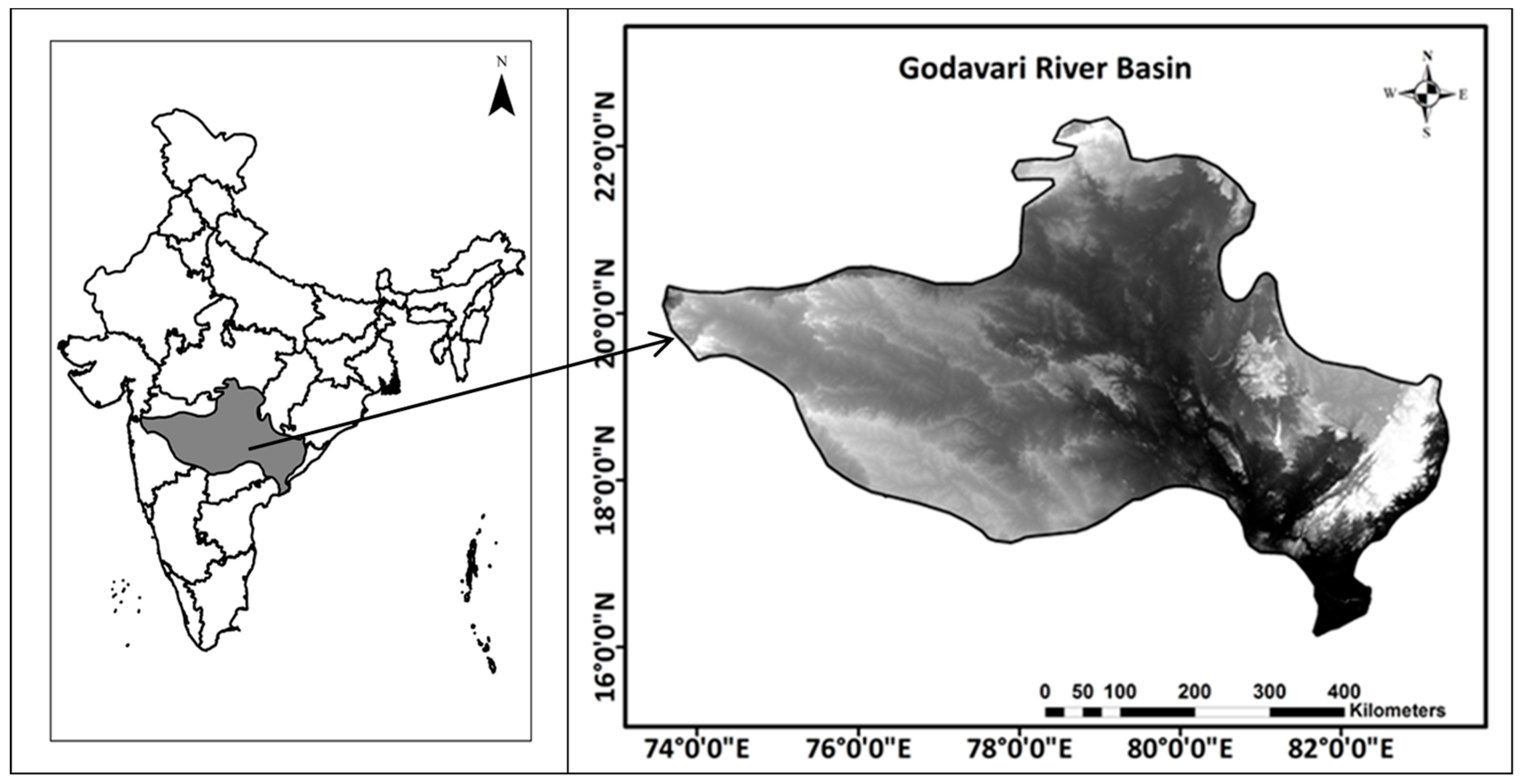
2. Study Area: The Godavari River Basin
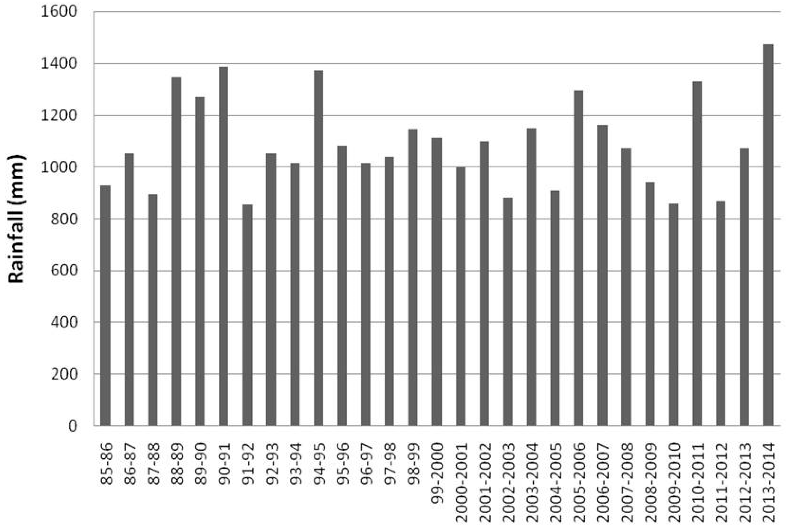
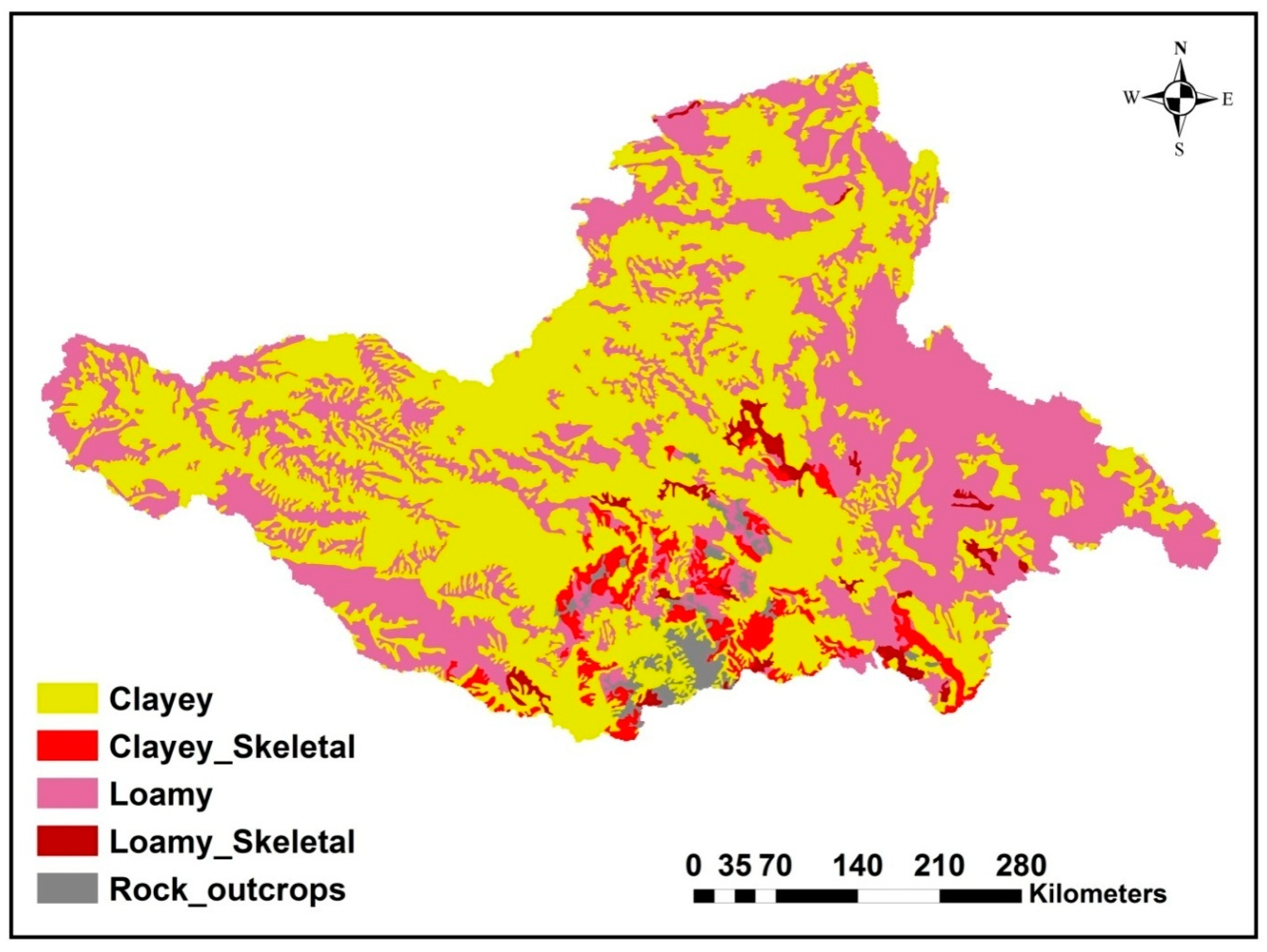
3. Data Used
4. Methodology
4.1. Land-Use and Land-Cover Classification
4.2. Accuracy Assessment
4.3. Land-Use and Land-Cover Change Detection Analysis
4.4. Hydrological Modeling Using the HEC-HMS Model 4.1
5. Results and Discussion
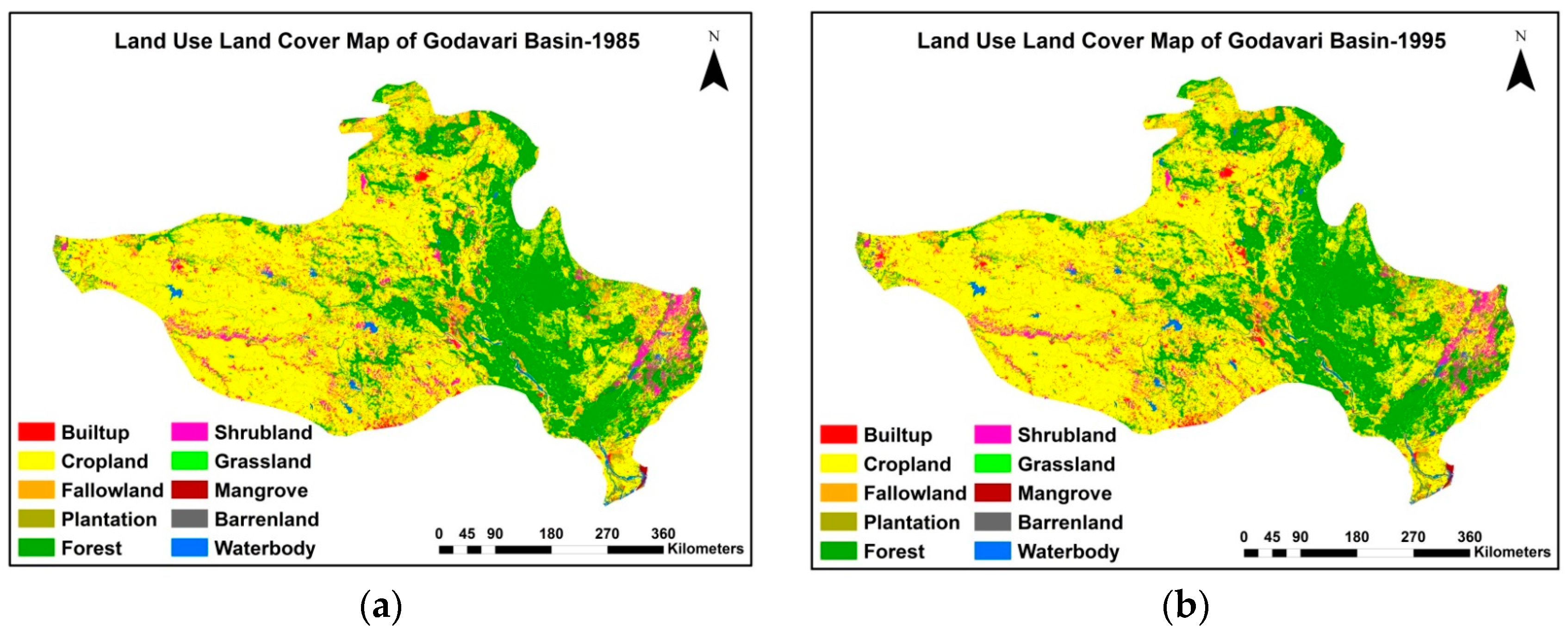
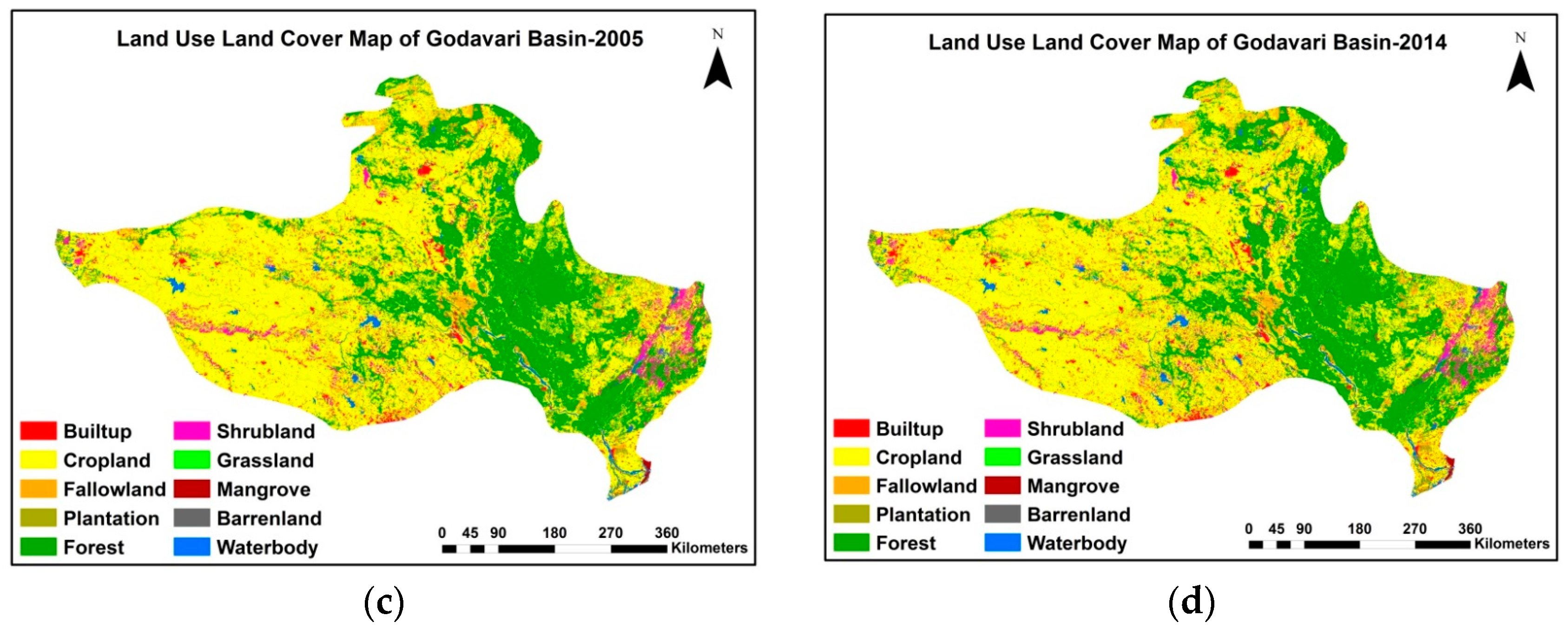
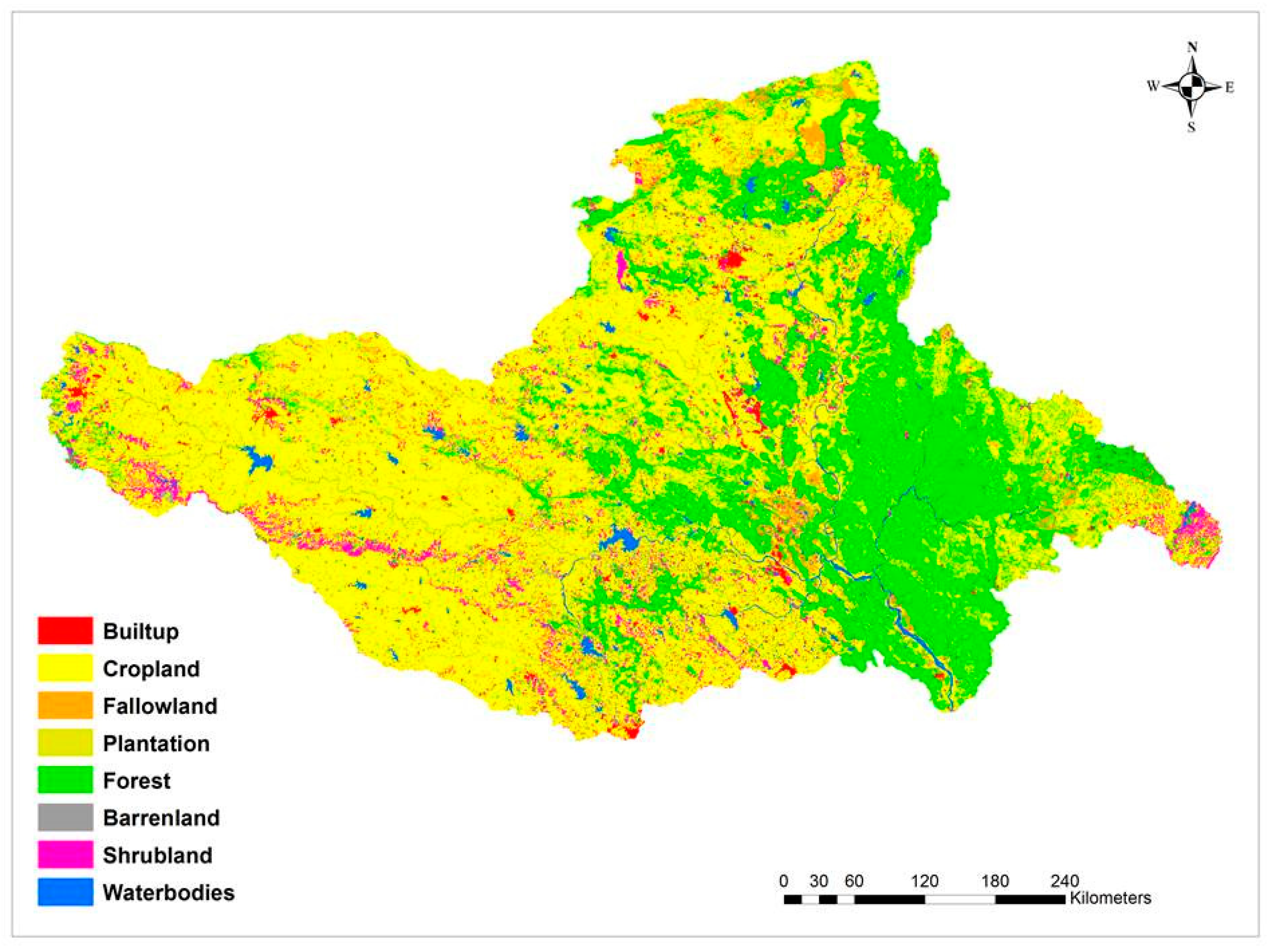
5.1. Land-Use and Land-Cover Map of Godavari Basin
5.2. Change Detection Analysis of the Godavari Basin
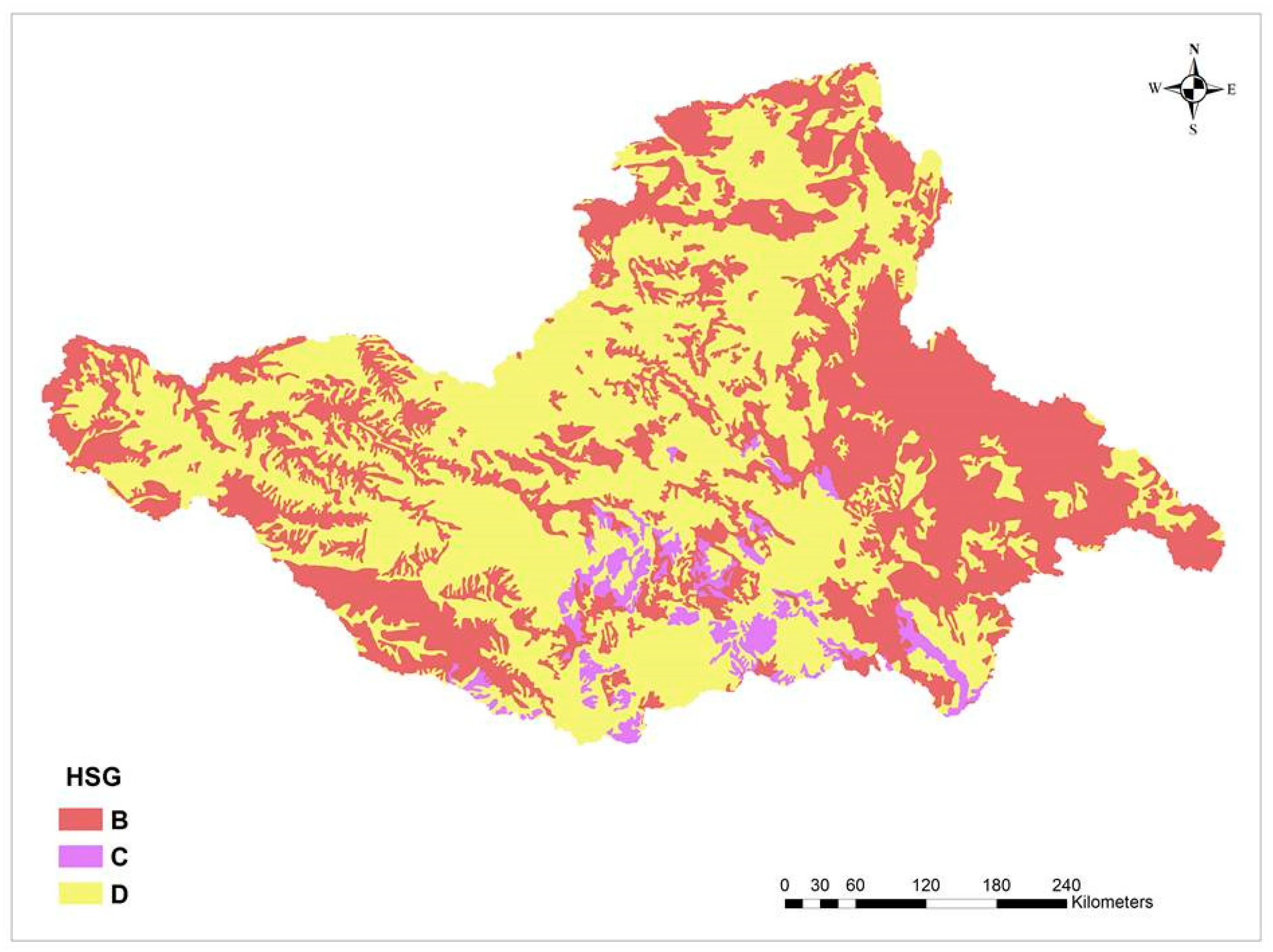
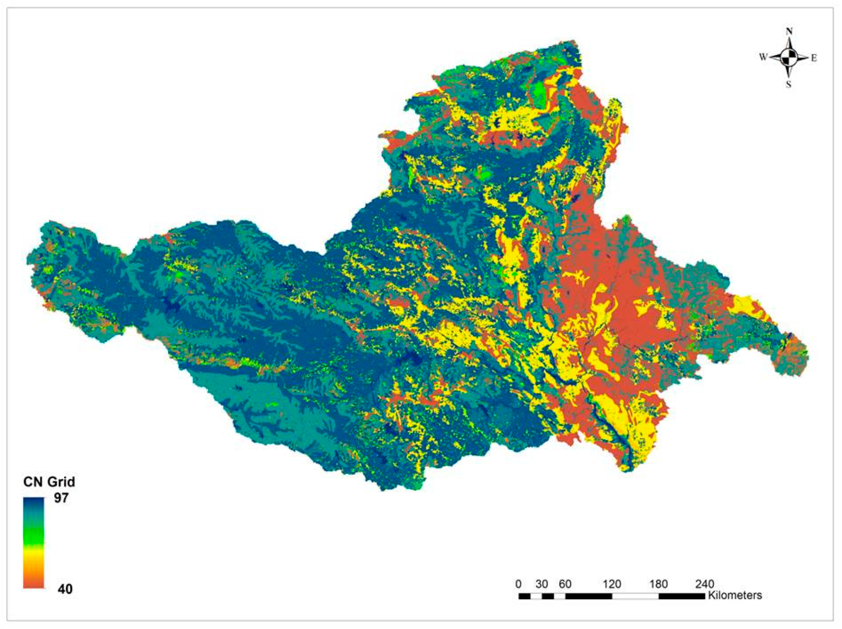
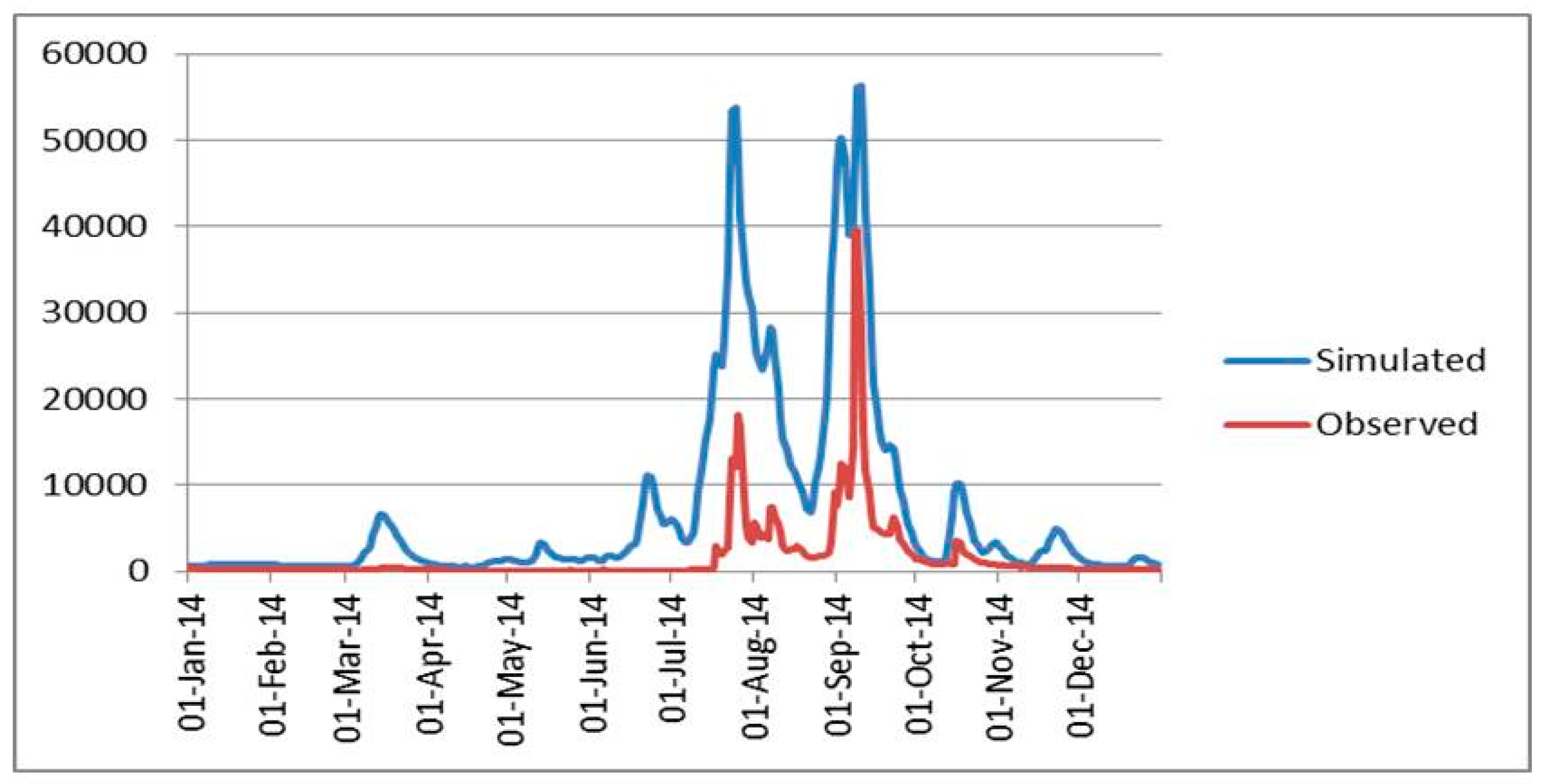
5.3. HEC-HMS Model of the Godavari River Basin
5.4. Impact of LULC Change on Runoff
6. Conclusions
Author Contributions
Acknowledgments
Conflicts of Interest
References
- Gautam, N.C.; Narayanan, L.R.A. Landsat MSS data for land use/land cover inventory and mapping: A case study of Andhra Pradesh. J. Indian Soc. Remote Sens. 1983, 11, 15–28. [Google Scholar]
- Sharma, K.R.; Jain, S.C.; Garg, R.K. Monitoring land use and land cover changes using Landsat imager. J. Indian Soc. Remote Sens. 1984, 12, 115–121. [Google Scholar]
- Brahabhatt, V.S.; Dalwadi, G.B.; Chhabra, S.B.; Ray, S.S.; Dadhwal, V.K. Land use/land cover change mapping in Mahi canal command area, Gujarat using multi-temporal satellite data. J. Indian Soc. Remote Sens. 2000, 28, 221–232. [Google Scholar] [CrossRef]
- Anil, Z.C.; Katyar, S.K. Impact analysis of open cast coal mines on land use/land cover using remote sensing and GIS technique: A case study. Int. J. Eng. Sci. Technol. 2010, 2, 7171–7176. [Google Scholar]
- Roy, P.S.; Roy, A. Land use and land cover change in India: A remote sensing & GIS perspective. J. Indian Inst. Sci. 2010, 90, 489–502. [Google Scholar]
- Anil, N.C.; Sankar, G.J.; Rao, M.J.; Prasad, I.V.; Sailaja, U. Studies on Land Use/Land Cover and change detection from parts of South West Godavari district, A.P–Using Remote Sensing and GIS Techniques. J. Indian Geophys. Union 2011, 15, 187–194. [Google Scholar]
- Kamal, P.; Kumar, M.; Rawat, J.S. Application of Remote Sensing and GIS in Land Use and Land Cover Change Detection: A Case study of Gagas Watershed, Kumaun Lesser Himalaya, India. Quest 2012, 6, 342–345. [Google Scholar] [CrossRef]
- Amin, A.; Fazal, S. Quantification of Land Transformation using Remote sensing and GIS Techniques. Am. J. Geogr. Inf. Syst. 2012, 1, 17–28. [Google Scholar] [CrossRef]
- Rawat, J.S.; Biswas, V.; Kumar, M. Changes in land use/cover using geospatial techniques: A case study of Ramnagar town area, Nainital district, Uttarakhand, India. Egypt. J. Remote Sens. Space Sci. 2013, 16, 111–117. [Google Scholar] [CrossRef]
- Rawat, J.S.; Kumar, M. Monitoring land use/cover change using remote sensing and GIS techniques: A case study of Hawalbagh block, district Almora, Uttarakhand, India. Egypt. J. Remote Sens. Space Sci. 2015, 18, 77–84. [Google Scholar] [CrossRef]
- Sampath Kumar, P.; Mahtab, A.; Roy, A.; Srivastava, V.K.; Roy, P.S.; ISRO, D. Impact of drivers on the Land use/land cover change in Goa, India. In Proceedings of the International Symposium, India Geospatial Forum, Hyderabad, India, 5–7 February 2014. [Google Scholar]
- Roy, P.S.; Roy, A.; Joshi, P.K.; Kale, M.P.; Srivastava, V.K.; Srivastava, S.K.; Dwevidi, R.S.; Joshi, C.; Behera, M.D.; Meiyappan, P.; et al. Development of Decadal (1985–1995–2005) Land Use and Land Cover Database for India. Remote Sens. 2015, 7, 2401–2430. [Google Scholar] [CrossRef]
- Lorup, J.K.; Refsgaard, J.C.; Mazvimavi, D. Assessing the effect of land use change on catchment runoff by combined use of statistical tests and hydrological modelling: Case studies from Zimbabwe. J. Hydrol. 1998, 205, 147–163. [Google Scholar] [CrossRef]
- Brown, D.G.; Pijanowski, B.C.; Duh, J.D. Modeling the relationships between land use and land cover on private lands in the Upper Midwest, USA. J. Environ. Manag. 2000, 59, 247–263. [Google Scholar] [CrossRef]
- Seneviratne, S.I.; Corti, T.; Davin, E.L.; Hirschi, M.; Jaeger, E.B.; Lehner, I.; Orlowsky, B.; Teuling, A.J. Investigating soil moisture-climate interactions in a changing climate: A review. Earth Sci. Rev. 2010, 99, 125–161. [Google Scholar] [CrossRef]
- Dadhwal, V.K.; Aggarwal, S.P.; Mishra, N. Hydrological Simulation of Mahanadi River Basin and Impact of Land Use/Land Cover Change on Surface Runoff Using a Macro Scale Hydrological Model. In Proceedings of the ISPRS TC VII Symposium—100 Years ISPRS, Vienna, Austria, 5–7 July 2010; Volume 38. [Google Scholar]
- Rao, K.H.V.D.; Rao, V.V.; Dadhwal, V.K.; Behera, G.; Sharma, J.R. A distributed model for real-time flood forecasting in the Godavari Basin using space inputs. Int J Disaster Risk Sci. 2012, 2, 31–40. [Google Scholar] [CrossRef]
- Asadi, A.; Sedghi, H.; Porhemat, J.; Babazadeh, H. Calibration, Verification and Sensitivity Analysis of the HEC-HMS Hydrologic Model (Study area: Kabkian Basin and Delibajak Watershed). Ecol. Environ. Conserv. 2012, 18, 805–812. [Google Scholar]
- Meenu, R.; Rehana, S.; Mujumdar, P.P. Assessment of hydrologic impacts of climate change in Tunga-Bhadra river basin, India with HEC-HMS and SDSM. Hydrol. Process. 2012, 27, 1572–1589. [Google Scholar] [CrossRef]
- Roy, D.; Begum, S.; Ghosh, S.; Jana, S. Calibration and Validation of HEC HMS Model for a River Basin in Eastern India. ARPN J. Eng. Appl. Sci. 2013, 8, 33–49. [Google Scholar]
- Jain, M.; Daman Sharma, S. Hydrological modeling of Vamsadhara River Basin, India using SWAT. In Proceedings of the International Conference on Emerging Trends in Image Processing, Pattaya, Thailand, 15–16 December 2014. [Google Scholar]
- Shinde, S.P.; Taley, S.M.; Kale, M.U. Hydrological Modeling with HEC-HMS for Wan Reservoir Catchment. Int. J. Agric. Sci. 2016, 8, 2263–2266. [Google Scholar]
- Leong, T.M.; Ibrahim, A.L.B. Remote Sensing, Geographic Information System and Hydrological Model for Rainfall—Runoff Modeling; ResearchGate Publication: Berlin, Germany, 2012. [Google Scholar]
- Halwatura, D.; Najim, M.M.M. Application of HEC HMS model for runoff simulation in a tropical catchment. Environ. Model. Softw. 2013, 46, 155–162. [Google Scholar] [CrossRef]
- Nirav Kumar, K.P.; Mukesh, K.T. Rainfall Runoff Modeling using Remote Sensing, GIS and HEC-HMS model. J. Water Resour. Pollut. Stud. 2017, 2, 1–8. [Google Scholar]
- Anderson, J.R. Land use classification schemes used in selected recent geographic applications of remote sensing. Photogramm. Eng. Remote Sens. 1971, 37, 379–387. [Google Scholar]
- Congalton, R.G.; Green, K. Assessing the accuracy of remote sensed data. Remote Sen. Environ. 1999, 37, 35–46. [Google Scholar] [CrossRef]
- Reddy, C.S.; Roy, A. Assessment of three decade vegetation dynamics in Mangroves of Godavari delta, India using multi-temporal satellite data and GIS. Res. J. Environ. Manag. 2008, 2, 108–115. [Google Scholar]
- NRCS-USDA. National Engineering Handbook; Part 630 Hydrology; Hydrological Soil Groups: Washington, DC, USA, 2009; Chapter 7.
- Subramanya, K. Engineering Hydrology, 4th ed.; McGraw-Hill Education Private Limited: New Delhi, India, 2013. [Google Scholar]
- Punnag, S. Estimation of Runoff of an Upper Catchment of an Existing Reservoir by SCS–CN Method Using GIS Software; IS-030-IA-LSCW: Phnom Penh, Cambodia, 2015; Chapter 3. [Google Scholar]


| LULC Class | 1985 | 1995 | 2005 | 2014 | ||||
|---|---|---|---|---|---|---|---|---|
| Area | ||||||||
| sq·km | % | sq·km | % | sq·km | % | sq·km | % | |
| Builtup | 1611 | 0.51 | 2253 | 0.72 | 2385 | 0.76 | 3611 | 1.15 |
| Cropland | 181,962 | 57.86 | 182,560 | 58.05 | 183,445 | 58.33 | 181,337 | 57.66 |
| Fallowland | 6584 | 2.09 | 6675 | 2.12 | 6860 | 2.18 | 6756 | 2.15 |
| Plantation | 1582 | 0.50 | 1589 | 0.51 | 1590 | 0.51 | 1716 | 0.55 |
| Forest | 92,851 | 29.52 | 92,361 | 29.37 | 92,237 | 29.33 | 92,273 | 29.34 |
| Shrubland | 18,808 | 5.98 | 17,152 | 5.45 | 15,957 | 5.07 | 15,907 | 5.06 |
| Grassland | 76 | 0.02 | 77 | 0.02 | 77 | 0.02 | 95 | 0.03 |
| Mangroves | 183 | 0.06 | 183 | 0.06 | 182 | 0.06 | 188 | 0.06 |
| Barrenland | 648 | 0.21 | 673 | 0.21 | 687 | 0.22 | 661 | 0.21 |
| Waterbodies | 10,198 | 3.24 | 10,980 | 3.49 | 11,083 | 3.52 | 11,959 | 3.80 |
| Total | 314,503 | 100 | 314,503 | 100 | 314,503 | 100 | 314,503 | 100 |
| Reference Data | |||||||||||
|---|---|---|---|---|---|---|---|---|---|---|---|
| Classified Data | FO | BU | CL | BL | GL | FL | PL | SL | WB | Total | |
| FO | 193 | 0 | 2 | 0 | 0 | 0 | 6 | 0 | 0 | 201 | |
| BU | 0 | 68 | 2 | 0 | 0 | 2 | 0 | 0 | 0 | 72 | |
| CL | 1 | 1 | 137 | 0 | 1 | 0 | 0 | 1 | 8 | 149 | |
| BL | 2 | 0 | 6 | 50 | 0 | 0 | 0 | 0 | 1 | 59 | |
| GL | 10 | 0 | 4 | 0 | 146 | 0 | 0 | 0 | 0 | 160 | |
| FL | 0 | 1 | 0 | 2 | 0 | 25 | 0 | 0 | 0 | 28 | |
| PL | 0 | 0 | 1 | 0 | 0 | 5 | 51 | 0 | 0 | 57 | |
| SL | 2 | 1 | 4 | 0 | 1 | 0 | 0 | 75 | 0 | 83 | |
| WB | 0 | 0 | 1 | 0 | 0 | 0 | 0 | 1 | 14 | 16 | |
| Total | 208 | 71 | 157 | 52 | 148 | 32 | 57 | 77 | 23 | 825 | |
| 1995 | 1985 | ||||||||||
| BU | CL | FL | PL | FO | SL | GL | MG | BL | WB | ||
| BU | 1611.30 | 0.00 | 0.00 | 0.00 | 0.00 | 0.00 | 0.00 | 0.00 | 0.00 | 0.01 | |
| CL | 325.20 | 180,662.40 | 24.46 | 4.43 | 9.77 | 246.01 | 0.64 | 0.00 | 2.45 | 686.17 | |
| FL | 0.01 | 0.02 | 6580.79 | 0.00 | 0.29 | 0.14 | 0.00 | 0.00 | 0.00 | 2.53 | |
| PL | 0.00 | 0.65 | 0.00 | 1581.54 | 0.00 | 0.00 | 0.00 | 0.00 | 0.00 | 0.05 | |
| FO | 19.38 | 417.82 | 4.45 | 0.17 | 92,345.13 | 21.05 | 0.00 | 0.00 | 0.00 | 42.81 | |
| SL | 297.43 | 1475.48 | 65.16 | 2.52 | 0.00 | 16,884.76 | 0.00 | 0.00 | 23.45 | 59.59 | |
| GL | 0.00 | 0.00 | 0.00 | 0.00 | 0.00 | 0.01 | 75.95 | 0.00 | 0.00 | 0.00 | |
| MG | 0.00 | 0.00 | 0.00 | 0.00 | 0.00 | 0.00 | 0.00 | 183.12 | 0.00 | 0.17 | |
| BL | 0.00 | 0.14 | 0.00 | 0.00 | 0.29 | 0.08 | 0.00 | 0.00 | 647.54 | 0.01 | |
| WB | 0.00 | 3.79 | 0.00 | 0.13 | 5.49 | 0.41 | 0.00 | 0.00 | 0.00 | 10,188.18 | |
| 2005 | 1995 | ||||||||||
| BU | CL | FL | PL | FO | SL | GL | MG | BL | WB | ||
| BU | 2253.12 | 0.20 | 0.00 | 0.00 | 0.00 | 0.00 | 0.00 | 0.00 | 0.00 | 0.00 | |
| CL | 85.98 | 181,751.03 | 109.02 | 1.35 | 20.22 | 270.06 | 0.00 | 0.15 | 0.89 | 321.61 | |
| FL | 5.00 | 60.67 | 6604.02 | 0.58 | 1.51 | 2.19 | 0.00 | 0.90 | 0.00 | 0.00 | |
| PL | 0.00 | 3.97 | 0.00 | 1578.61 | 0.59 | 0.69 | 0.00 | 0.13 | 4.67 | 0.13 | |
| FO | 0.00 | 153.52 | 2.62 | 0.00 | 92,196.12 | 0.98 | 0.00 | 0.00 | 0.08 | 7.64 | |
| SL | 31.11 | 1219.06 | 135.52 | 6.33 | 11.09 | 15,678.65 | 0.00 | 0.00 | 0.87 | 69.84 | |
| GL | 0.00 | 0.00 | 0.00 | 0.00 | 0.00 | 0.00 | 76.59 | 0.00 | 0.00 | 0.00 | |
| MG | 0.02 | 0.00 | 1.76 | 0.01 | 0.00 | 0.00 | 0.00 | 171.20 | 0.52 | 9.62 | |
| BL | 0.00 | 5.30 | 0.00 | 0.00 | 0.00 | 0.00 | 0.00 | 0.00 | 668.02 | 0.12 | |
| WB | 9.44 | 251.08 | 7.33 | 3.38 | 7.15 | 4.93 | 0.00 | 9.79 | 12.05 | 10,674.38 | |
| 2014 | 2005 | ||||||||||
| BU | CL | FL | PL | FO | SL | GL | MG | BL | WB | ||
| BU | 2383.61 | 0.00 | 0.00 | 0.00 | 0.00 | 0.00 | 0.00 | 0.00 | 0.00 | 1.05 | |
| CL | 973.35 | 180,736.75 | 76.67 | 62.30 | 272.74 | 58.63 | 0.26 | 0.00 | 21.51 | 1242.53 | |
| FL | 70.01 | 86.02 | 6653.40 | 4.51 | 0.34 | 4.66 | 0.00 | 0.01 | 1.83 | 39.49 | |
| PL | 25.01 | 15.24 | 0.65 | 1537.88 | 4.33 | 4.21 | 0.00 | 0.07 | 0.00 | 2.88 | |
| FO | 20.94 | 19.87 | 5.75 | 57.82 | 91,869.15 | 25.61 | 22.01 | 0.00 | 5.73 | 209.80 | |
| SL | 63.42 | 30.61 | 2.46 | 0.18 | 17.73 | 15,761.23 | 1.40 | 0.00 | 15.85 | 64.61 | |
| GL | 0.00 | 0.91 | 0.00 | 0.00 | 4.08 | 0.00 | 71.61 | 0.00 | 0.00 | 0.00 | |
| MG | 0.60 | 0.19 | 0.52 | 0.37 | 0.00 | 0.00 | 0.00 | 173.38 | 0.00 | 7.11 | |
| BL | 0.64 | 27.33 | 0.91 | 11.09 | 2.42 | 23.28 | 0.00 | 1.43 | 603.48 | 16.53 | |
| WB | 73.78 | 419.87 | 15.48 | 42.25 | 102.00 | 29.54 | 0.00 | 12.78 | 12.81 | 10,374.83 | |
| LU Value | Description | Soil A | Soil B | Soil C | Soil D |
|---|---|---|---|---|---|
| 1 | Built up | 49 | 69 | 79 | 84 |
| 2 | Cropland | 76 | 86 | 90 | 93 |
| 3 | Fallowland | 54 | 70 | 80 | 85 |
| 4 | Plantation | 41 | 55 | 69 | 73 |
| 5 | Forest | 26 | 40 | 58 | 61 |
| 6 | Shrubland | 33 | 47 | 64 | 67 |
| 7 | Barrenland | 71 | 80 | 85 | 88 |
| 8 | Waterbodies | 97 | 97 | 97 | 97 |
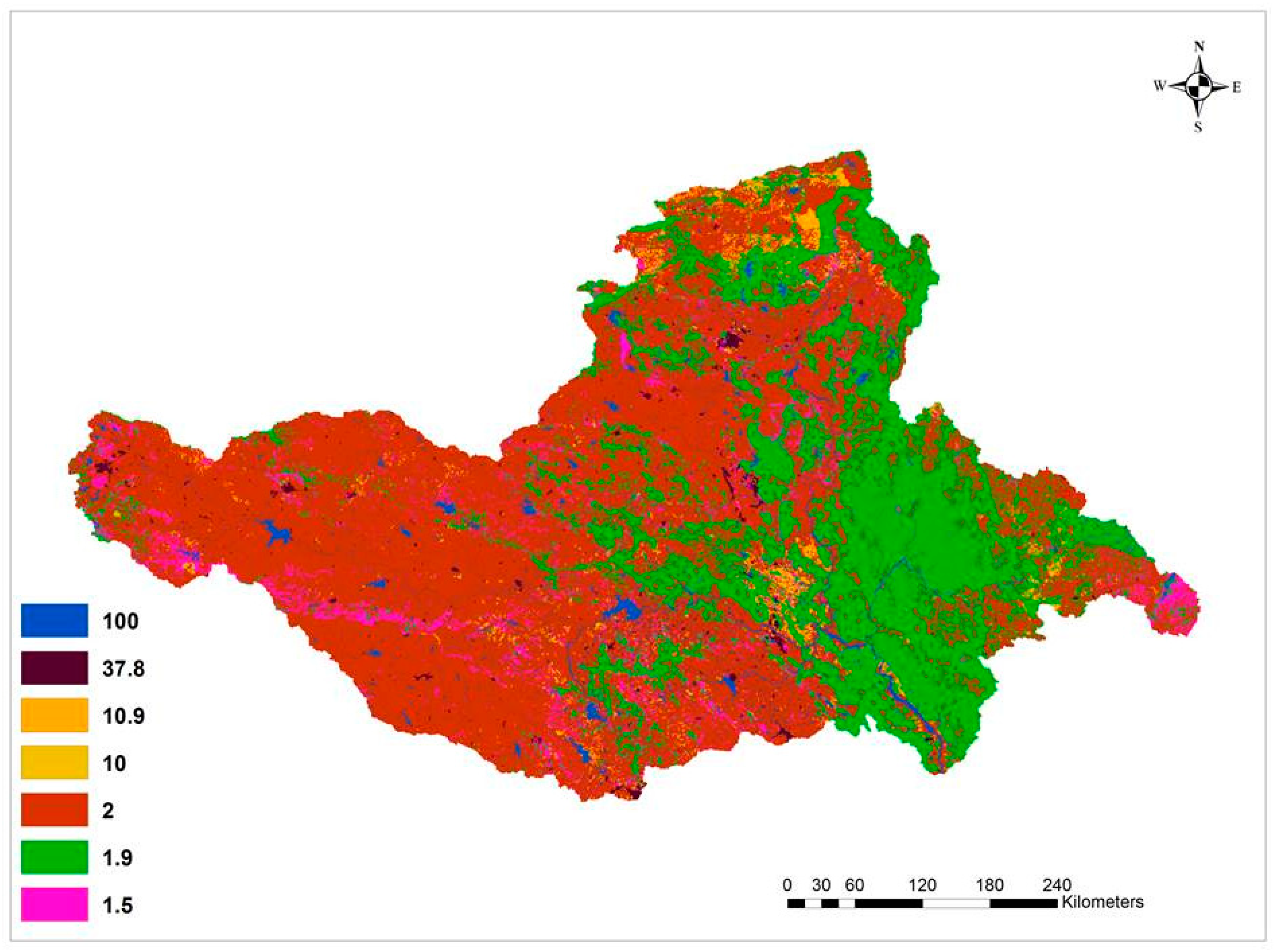
| Land Use | % Imperviousness |
|---|---|
| Builtup | 37.8 |
| Cropland | 2 |
| Barrenland | 10 |
| Forest | 1.9 |
| Fallowland | 10.9 |
| Plantation | 1.9 |
| Shrubland | 1.5 |
| Waterbodies | 100 |
| LULC Class | 1985 | 1995 | 2005 | 2014 |
|---|---|---|---|---|
| Area Sq·Km | ||||
| Builtup | 128 | 206 | 214 | 323 |
| Cropland | 6187 | 6392 | 6427 | 6283 |
| Fallowland | 368 | 367 | 410 | 397 |
| Plantation | 5 | 5 | 5 | 4 |
| Forest | 4451 | 4307 | 4306 | 4298 |
| Shrubland | 796 | 626 | 554 | 545 |
| Barrenland | 11 | 11 | 12 | 17 |
| Waterbodies | 789 | 821 | 807 | 868 |
© 2018 by the authors. Licensee MDPI, Basel, Switzerland. This article is an open access article distributed under the terms and conditions of the Creative Commons Attribution (CC BY) license (http://creativecommons.org/licenses/by/4.0/).
Share and Cite
Koneti, S.; Sunkara, S.L.; Roy, P.S. Hydrological Modeling with Respect to Impact of Land-Use and Land-Cover Change on the Runoff Dynamics in Godavari River Basin Using the HEC-HMS Model. ISPRS Int. J. Geo-Inf. 2018, 7, 206. https://doi.org/10.3390/ijgi7060206
Koneti S, Sunkara SL, Roy PS. Hydrological Modeling with Respect to Impact of Land-Use and Land-Cover Change on the Runoff Dynamics in Godavari River Basin Using the HEC-HMS Model. ISPRS International Journal of Geo-Information. 2018; 7(6):206. https://doi.org/10.3390/ijgi7060206
Chicago/Turabian StyleKoneti, Sunitha, Sri Lakshmi Sunkara, and Parth Sarathi Roy. 2018. "Hydrological Modeling with Respect to Impact of Land-Use and Land-Cover Change on the Runoff Dynamics in Godavari River Basin Using the HEC-HMS Model" ISPRS International Journal of Geo-Information 7, no. 6: 206. https://doi.org/10.3390/ijgi7060206