Direction-Aware Continuous Moving K-Nearest-Neighbor Query in Road Networks

1
College of Computer Science and Technology, Zhejiang University of Technology, Hangzhou 310023, China
2
School of Economics and Management, Zhejiang University of Science and Technology, Hangzhou 310023, China
*
Author to whom correspondence should be addressed.
ISPRS Int. J. Geo-Inf. 2019, 8(9), 379; https://doi.org/10.3390/ijgi8090379
Submission received: 29 May 2019
/
Revised: 23 July 2019
/
Accepted: 21 August 2019
/
Published: 29 August 2019
(This article belongs to the Special Issue Spatial Big Data, BIM and advanced GIS for Smart Transformation: City, Infrastructure and Construction)
Abstract
:Continuous K-nearest neighbor (CKNN) queries on moving objects retrieve the K-nearest neighbors of all points along a query trajectory. They mainly deal with the moving objects that are nearest to the moving user within a specified period of time. The existing methods of CKNN queries often recommend K objects to users based on distance, but they do not consider the moving directions of objects in a road network. Although a few CKNN query methods consider the movement directions of moving objects in Euclidean space, no efficient direction determination algorithm has been applied to CKNN queries over data streams in spatial road networks until now. In order to find the top K-nearest objects move towards the query object within a period of time, this paper presents a novel algorithm of direction-aware continuous moving K-nearest neighbor (DACKNN) queries in road networks. In this method, the objects’ azimuth information is adopted to determine the moving direction, ensuring the moving objects in the result set towards the query object. In addition, we evaluate the DACKNN query algorithm via comprehensive tests on the Los Angeles network TIGER/LINE data and compare DACKNN with other existing algorithms. The comparative test results demonstrate that our algorithm can perform the direction-aware CKNN query accurately and efficiently.
1. Introduction
There are many LBS applications, such as taxi hailing, ride sharing and car navigation, and various K-nearest-neighbor (KNN) query algorithms have been proposed to solve these problems. With the development of geographic information systems (GISs), KNN query in road networks has evolved from static objects to dynamic objects. The moving objects change their locations and directions frequently over time; therefore, the cost of retrieving the exact results of continuous K-nearest neighbor (CKNN) for moving objects is expensive, particularly in highly dynamic spatio-temporal applications, for example, finding the nearest taxi while the user moves in road networks over a period of time. When the user moves to a new location, the traditional solution is to perform a snapshot KNN query. Due to the objects’ continuous movement in road networks, a series of frequent snapshot KNN queries are necessary, which are unrealistic and expensive. The cost includes updating the location of moving objects when the velocities change over time and processing the CKNN queries that are posed by the moving object to the server. Therefore, this paper proposes a continuous KNN query method for predicting the K-nearest moving objects via predictive computation.
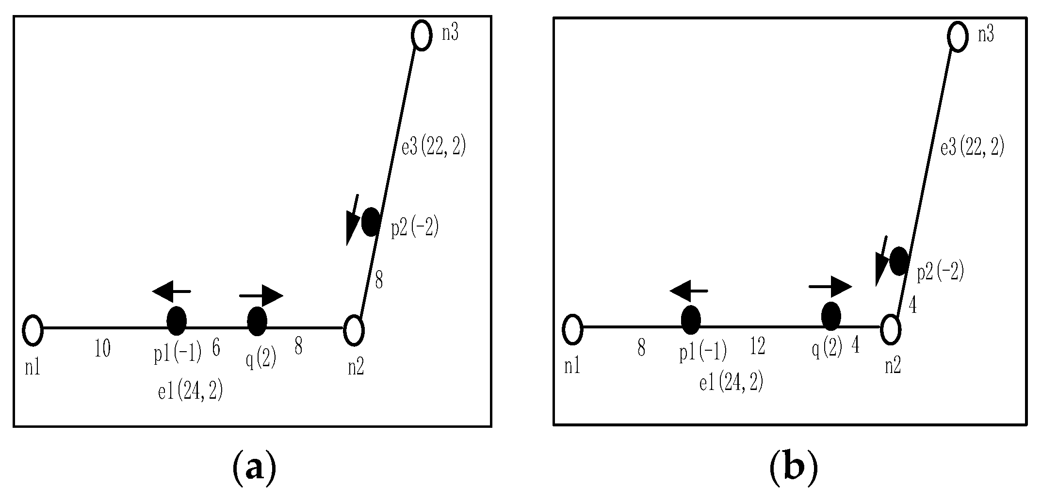
As shown in Figure 1, there are a query object, which is denoted by q, and a moving object set, which is denoted by P. Each object in the road network moves in the direction of arrow. Taking the query object q as an example, q(2) indicates that the query object q moves at speed 2 towards starting point n2 of the edge where q is located in the road network. The moving query object q requests to retrieve the nearest neighbor object in a specified period. In Figure 1a, the result of the nearest- neighbor query is p1 at timestamp 0, and the query result is changed to p2 at timestamp 2, as shown in Figure 1b. The query system must monitor the timestamp when the query result will change in the time interval [0, 2] and return the updated result. The query result consists of two-tuples, <{p1}, [t0, t1]>, <{p2}, [t1, t2]>… <{pi}, [ti-1, ti]>. {pn}, [tn-1, tn]. The query results in Figure 1 are as follows: <{p1}, [0, 10/7]> and <{p2}, [10/7, 2]>.
As in Figure 1, the CKNN query only uses distance as the criterion, namely, the KNN query recommended objects are the nearest objects to the query object; however, there may be objects that move away from the query object gradually and the distance to the query object will increase. Moreover, in one-way roads, these moving objects need to turn around at the next intersection to reach the query object. For identifying the object that is nearest to the query object in application scenarios, the object that is queried in Figure 1a is invalid. Therefore, the CKNN query should not only consider the distance factor but also the direction of moving objects. In this paper, we propose a method of direction-aware continuous moving K-nearest neighbor (DACKNN) query in road networks. By using the direction constraint, we can continuously monitor the K-nearest moving objects that are moving towards the query object.
Many scholars [1,2,3] have utilized the search-space pruning algorithm, which is based on a road network, to deal with continuous K-nearest neighbor queries. Most of them only consider the nearest objects in the dimension of distance. There are some scholars [4,5,6] that consider the direction-aware query of moving objects in Euclidean space. However, the problem does not involve road network constraints; hence, it cannot be applied to continuous nearest-neighbor query in road networks. In this paper, we consider direction-aware continuous nearest-neighbor queries under the following three assumptions: (1) all objects (including the query object) are dynamic in the road network. (2) The distance between two objects is represented by the shortest path between the two objects in the road network. (3) The result set in each sub-interval of a period is determined. The first problem to be solved is the calculation of the distances between moving objects and the query object at every timestamp in the road network. Because of the continuous movement of objects in the road network, the distance between any two objects is constantly changing. If the Dijkstra algorithm is used for every movement change, the re-computation of the network distance is highly time-consuming. In this paper, the distance between moving objects is calculated based on three factors: the moving speed, the moving direction, and the shortest path between the nodes in the road network. It is a linear function of time.
The main contributions of this paper are as follows:
- The directions of the moving objects are considered to guarantee that the objects in the result set move towards the query object to realize the direction-aware CKNN.
- The concept of monitoring distance is proposed to determine which moving object affects the CKNN query results.
- This paper evaluates the DACKNN algorithm via comprehensive tests on the Los Angeles network TIGER/LINE data and the comparative test results demonstrate the efficiency and practicability of our DACKNN algorithm.
In this paper, Section 2 introduces the related work on the K-nearest-neighbor query in road networks; Section 3 presents the data structure, problem definition and related concepts; Section 4 describes the direction-aware continuous moving K-nearest-neighbor query algorithm in a road network environment; Section 5 presents the results and analyses of the relevant comparative tests; and Section 6 summarizes the paper, identifies the shortcomings and discusses future work.
2. Related Work
Shifting from static objects to dynamic objects, many scholars focused on CKNN queries under road network constraints. However, the practical requirements of users are not met by only considering the distance factor. Therefore, the direction-based CKNN query will inevitably become a trend in spatial database technology.
2.1. K-Nearest-Neighbor Query in Road Networks
The K-nearest-neighbor query in road networks has been widely studied in the field of spatial databases. Papadias et al. [7] proposed a flexible system for handling KNN queries in spatial road network databases, which used the Incremental Euclidean Restriction (IER) algorithm and the Incremental Network Expansion (INE) algorithm to discover KNN objects. These extensions are inspired by the Dijkstra algorithm [8]. Kolahdouzan et al. [9] introduced the Network Nearest Neighbor (VN3) algorithm for solving KNN queries by dividing the spatial network into several small voronoi polygons, and calculated the road network distance based on these voronoi polygons. Hu et al. [10,11] facilitated the KNN query by establishing an index. The KNN query was performed by retrieving a set of interconnected trees [10]. These trees come from the road network. Hu et al. [11] used the distance labeling to maintain approximate road network distances and construct indices to accelerate KNN search. Lee et al. [12] pruned the KNN search space into a subspace without objects. The above studies only consider the distances in the road network as the criterion for judging the neighborhoods; however, in practice, the distance between moving objects cannot be determined only by the physical distance and the relative direction of motion between the two is also an important factor.
2.2. Continuous K-Nearest-Neighbor Query in Road Networks
With the rapid development of moving devices, the motion states of moving objects in space can be monitored in real time. We are no longer satisfied with KNN query in static environments. The KNN query in dynamic environments has attracted more attention and CKNN query has become a research hotspot. The query results of CKNN query processing are computed continuously in the specified period by moving users; thus, the process is highly complicated.
Tao et al. [1] designed a CKNN query processing method for a line edge. This query processing method uses R-tree as the underlying data structure and the KNN query results of a query object on a line can be obtained via a single calculation; however, this method can only query on a pre-defined line. The authors in [2,3] solved the CKNN query for a moving query location on the query path. Cho et al. [2] employed the unique continuous search algorithm which divides the query path into effective intervals by considering the distance between the object and the query object. Within each interval, regardless of where the query moves, the KNN object is the same. Kolahdouzan et al. [3] introduced the IE/UBA algorithm for identifying CKNN candidates and divided paths into several sub-paths, each of which has the same KNN result set. The objects that are queried in [2,3] are static on the road network; only the query object can move on the path. Since the object that is being queried is moving, Shahabi et al. [13] developed a Road Network Embedding (RNE) technique, which transforms the road network into a higher-dimensional space, retrieves approximate results, and mainly deals with CKNN queries of moving objects on the road network. Mouratidis et al. [14] proposed the incremental monitoring algorithm (IMA) and group monitoring algorithm (GMA) algorithms for updating the results when updates from objects and edges falling in the expansion tree. Demiryurek et al. [15] extended the method for solving the same problem in [14]. The proposed ER-CKNN algorithm avoids blindly expanding the road network when searching for candidate objects and selects candidate objects based on the Euclidean distance between each object and the query object. Huang et al. [16] developed a continuous K-nearest-neighbor query algorithm (CKNN) for moving objects in road networks. This algorithm uses a continuous detection method for moving objects in road networks, eliminates unqualified moving objects and identifies candidate objects, and evaluates candidate objects to determine whether they belong to the K-nearest neighbors of the query objects. Li et al. [17] introduced a continuous KNN (SCKNN) algorithm that is based on a moving state value. This algorithm considers the continuous K-nearest-neighbor queries of query object and the moving objects’ moving states, identifies fewer candidate objects, and increases the computational efficiency. Although the existing continuous K-nearest-neighbor query method considers the distance attributes and the motion state of the object, it does not consider the moving direction of the moving object relative to the query object; thus, it cannot accurately realize continuous K-nearest-neighbor query towards the query object.
2.3. Direction-Based KNN Query
In the spatial database query, researchers have introduced direction attributes and carried out some researches on direction-based spatial query technology. To improve the efficiency of direction determination, an open shape-based strategy (OSS) model proposed by Liu et al. [4], which transforms the direction determination between geometric objects and query objects into a spatial topology analysis between open-shape and closed-geometric objects and improves the query efficiency. Patroumpas [5] solved the range query problem of objects that are moving towards query objects in Euclidean space. To quickly determine whether the moving objects are moving towards the query object, a Polar-Tree is generated for each query object via polarization mapping with query objects as poles to efficiently complete the range query and the objects in the result set are moving towards the query object. However, this method can only be applied to scenarios in which the query object is fixed and known and cannot handle random query requests. Nutanong et al. [6] studied visible K-nearest neighbor (VkNN) queries. The main problem is to identify the neighbors that can be seen by the query object; objects that are blocked by obstacles should be excluded. Gao et al. [18] studied the continuous visible K-nearest neighbor (CVkNN) queries, in which the query object can move along a straight edge and the algorithm returns the visible K-nearest object at any point on the edge. The main strategy of CVkNN is to perform only one single-point query for the whole edge instead of one query for each point of the edge. At the same time, an efficient heuristic strategy is used to prune the interest point set and the obstacle set separately, which substantially improves the query efficiency.
Li et al. [19] solved the K-nearest-neighbor query problem in the perspective direction of query object using direction-aware spatial keyword search. Given the location of the query object and the viewing angle range, the algorithm returns the K-nearest neighbors within the viewing angle range. View-field K-nearest-neighbor (VFkNN) query, which was proposed by Yi et al. [20], solves similar problems to direction-aware spatial keyword search; however, and VFkNN supports query processing of moving objects. This method uses a grid to index interest points, accesses the grid within the perspective, and directly excludes the grid outside the perspective, which substantially increases the query efficiency. Because of the high applicability of the grid index to moving objects, the VFkNN algorithm can not only process queries of static interest points but also fully support moving interest points. At the same time, they also solve the problem of continuous VFkNN query. Continuous VFkNN query is divided into two stages: an initial stage and an update stage. In the initial stage, the author implements two query algorithms, namely, naive search and sector search, which are used to process snapshot VFkNN queries. In the update stage, the sector surveillance algorithm, which is proposed in this paper, can efficiently handle the updating of moving objects. Lee et al. [21,22,23] studied the nearest surrounder (NS) query. No longer is only the interest point that is nearest to the query object identified; multiple interest points are returned. These interest points are centered on the query object, distributed in various directions of query object and have a unique interest point in each direction. These interest points become the surroundings of the query object, that is to say, NS gives the query object a global perspective, from which the nearest-neighbor object to the query object in any direction can be identified. Guo [24] and others proposed Direction-Based Surrounder (DBS) queries for solving NS queries in Euclidean space and road network space and supporting continuous DBS query processing. Lee et al. [25] solved the K-nearest-neighbor query problem with the same direction as the query object by using a direction-constrained K-nearest-neighbor (DCkNN) query. Given the location and direction of query object, DCkNN can identify a point in the direction of the query object from the set of interest points if the difference value does not exceed a specified threshold, which is denoted as θ. Chen et al. [26] determined the nearest-neighbor query of the path and retrieved the nearest-neighbor object along the path of the query object.
Although these KNN query methods consider the direction attribute, the solved problems do not involve road network constraints or continuous moving K-nearest-neighbor query. Therefore, we propose a direction-aware continuous moving K-nearest-neighbor query algorithm in road networks that is based on progressive network expansion. Our previous research has solved the problem of Direction-aware KNN queries for moving objects in a road network (DAKNN) [27]. In this paper, we focused on the problem of continuous queries and the efficiency of continuous K-nearest-neighbor query for moving objects in road networks that are moving towards query objects.
3. Data Structure and Problem Definition
In this section, we present important concepts and data structures that are involved in directional-aware continuous moving K-nearest neighbor queries and formally define the problem that we attempt to solve in the paper.
3.1. Data Structure
In our method, it is assumed that the speed of each object that is moving in road networks is constant. The data structures are designed as follows.
The road network is composed of nodes and edges, which is represented by an undirected weighted graph, namely, G (N, E, W), where N represents the set of nodes and stores all node information of the road network; E represents the set of edges and stores the edges of the road network; W represents the weight of the edge, where the weight that is set by the system is the length of the edge [27]. In addition, the two endpoints of a specified edge are denoted by and . ns represents the starting point and ne represents the ending point of the edge. For simplicity, we do not consider the direction of each edge; therefore, the starting points and ending points of the edges in the road network are represented by only two endpoints, which are arbitrarily specified.
The moving objects are a set , where is a moving object p in the road network at timestamp t. The spatial information for each moving object in the road network, such as its location, speed, and movement direction at a timestamp, is available. Especially, when the moving object reaches a road network node, an adjacent edge of the node is randomly selected as its next traveling edge, the moving object will travel along the selected edge.
The query object refers to the spatial object that makes the query request, such as when a pedestrian makes the following query request: “At a certain period of time, find two taxis coming toward me.” In this case, the pedestrian is the initiator of the query request, namely, the query object. The query object typically contains the following information: (1) the query coordinates; (2) the query time interval; (3) the value of K; and (4) the result set.
Given a range value m, starting from the query object, the node is gradually expanded until the distance from all adjacent nodes of the current node to query object is greater than the range value m. Expanded edges constitute the influencing edge, which is composed of triples , where represents the distance between the node and .
In our algorithm, a data structure of memory is used to store edge, node and moving object information [27].
- Edge table: the following information is stored: (1) the edge starting and ending nodes; (2) the lengths of the edges; (3) the sets of objects that are moving on the edges; (4) the directions of the edges; and (5) the maximum speed.
- Node table: this mainly includes the node identifiers and the location information.
- Moving object table: the following information is stored: (1) the edge of the object; (2) the moving speed; (3) the distance to the starting node; (4) whether it moves towards the ending point; (5) the moving direction of the object; and (6) the time when the location of the object is updated.
3.2. Road Network Distance
The distance between two objects on an undirected weighted graph is the length of the shortest path. If two objects are not reachable, the distance is ∞.
In this paper, we must determine the road network distances between moving objects at each timestamp in the time interval. The distance between the moving object p and the query object q is denoted as . When the object arrives at the network node, the network distance must be recalculated. If the query object q and the moving object p are specified, the distance between them in any time interval can be calculated. According to the edge of the moving object and the location of the query object, there are two cases.
In the first case, the query object and the moving object move on the same edge, namely e, and the distance is calculated as follows:
In an undirected weighted graph, the starting and ending nodes are arbitrarily specified on each edge. If the object moves towards the ending node, indicates the positive speed; otherwise, indicates the negative speed. and represent the marking speed and the last update time, respectively, of the query object. Similarly, and represent the marking speed and the last update time, respectively, of the moving object. represents the distance between the query object and the starting point of the edge that is located by the query object. When an object arrives at the road network node, the distance between the object and the query object must be recalculated.
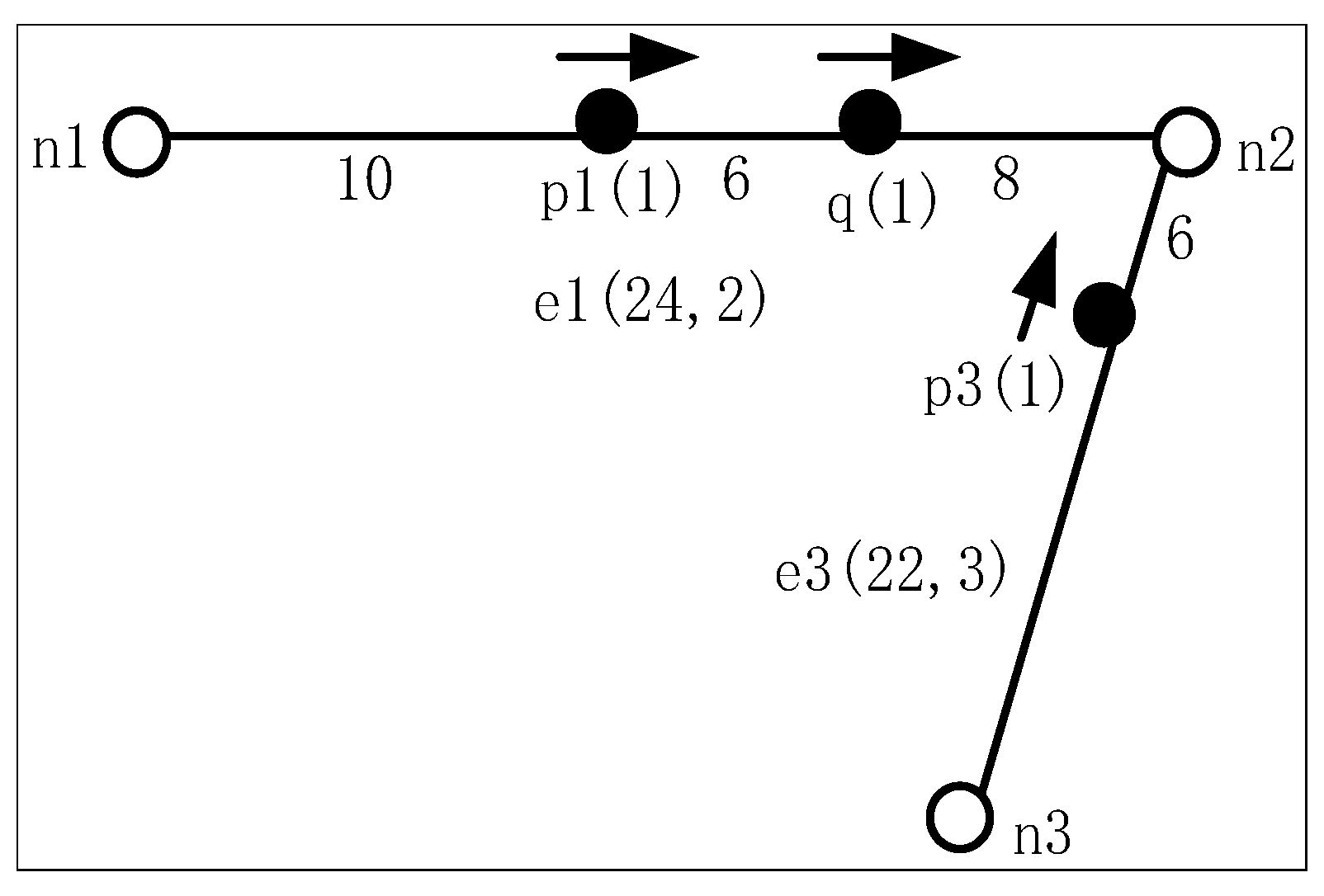
In the second case, query object q and the moving object p move on different edges, e.g., edge and edge . For simplicity, in this paper, we pre-calculate the shortest distance between the nodes in the road network and use to represent the shortest path between nodes and . In this case, the distance between objects can be calculated by the shortest path between nodes. The shortest paths between the starting nodes and the ending nodes of the two moving objects are denoted as , , , and . Therefore, the distance between the moving object and the query object at timestamp t is composed of the following three parts: (1) the distance between the query object and node or ; (2) the shortest path between the nodes; and (3) the distance between the moving object and node or . The road network distance can be expressed as:
where represents the distance between the object and the starting point of the edge and represents the distance between the object and the ending point of the edge. For example, in Figure 2, the paths are composed of edges and . The moving object, namely, p3, and the query object, namely, q, are located at and , respectively. The object p3 moves towards the starting point, namely, n2; hence, is . The query object q moves towards the ending point, namely, n2; hence, is . The distance between them is . We can find that when the moving object arrives at the node, its moving edge will change, and the four nodes involved in the distance calculation formula also change; thus, once the moving object reaches the node, its distance formula to the query point needs to be recalculated.
3.3. Problem Definition
After the above overview and basic definitions, we define the problem that is considered in this paper.
Question Definition: In this paper, we study direction-aware continuous moving KNN queries in road networks in dynamic environments.
In a dynamic environment, if there is a group of moving objects P and a query object q in the road network, the query is to retrieve the K-nearest neighbors from the road network at any timestamp in [t0, t1] towards the query object, e.g., “A moving passenger inquires about K taxis moving towards himself during [t0, t1] period”.
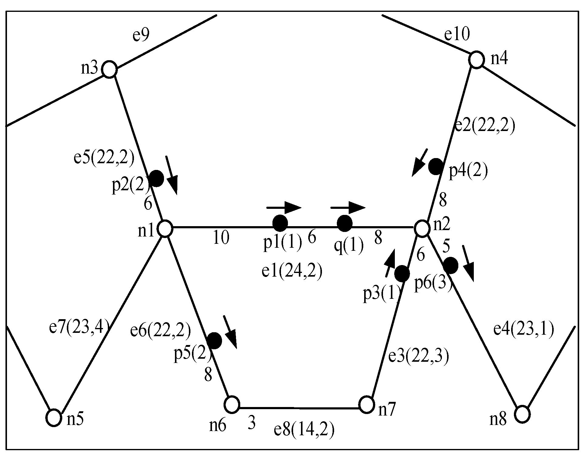
For the example in Figure 3, the global problem is clarified. In edge , represents the length of the edge and represents the speed limit of indicating the maximum speed of the moving object on . For moving object p(s), s represents the speed of object p. The query point q requests the two nearest-neighbor objects in the time interval [0, 4].
4. Direction-Aware Continuous Moving K-Nearest Neighbor Query
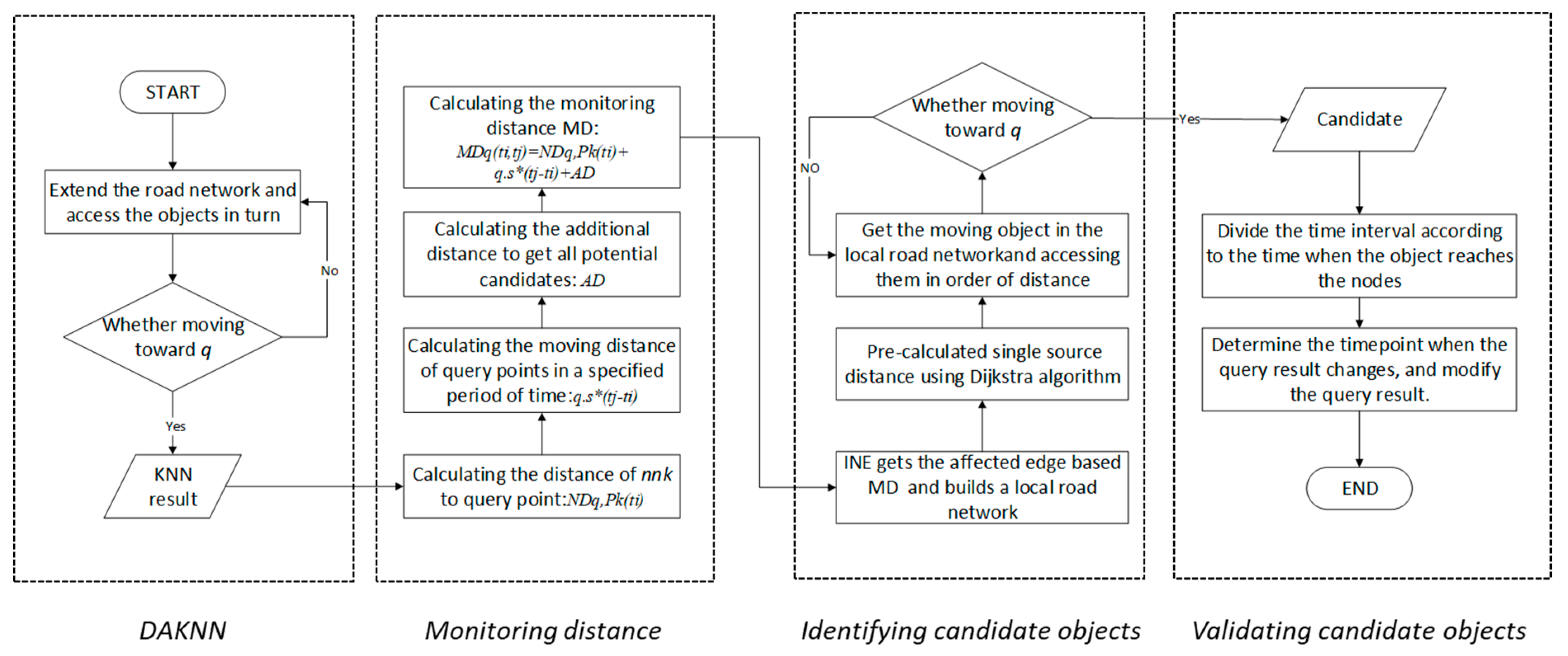
When the query object arrives at the road network node, it records the timestamp and divides the time interval into sub-intervals such that in each sub-interval, the query object moves on the same edge. First, we must execute the direction-aware KNN query algorithm at the starting timestamp to identify the K-nearest neighbor objects that are moving towards the query object. Then, the monitoring range of continuous queries is calculated; the moving objects in the monitoring range may affect the query results. After that, a local road network is established according to the monitoring range and then moving candidates are identified. Finally, the timestamp when the candidate objects replace the query results is determined. If the timestamp is within the specified period, the sub-interval is divided, and the result set is modified. Figure 4 shows the basic process of the algorithm.
4.1. Direction-Aware K-Nearest Neighbor Query for Moving Objects
In determining whether the moving object moves towards query object in road networks, two cases are considered. Case 1: the moving object and the query object are on the same edge. At this time, it is only necessary to determine whether the moving direction of the moving object points towards the query object or not. The moving direction of the moving object is determined according to the azimuth information. Case 2: the moving object and the query object are on the different edge. This paper adopts the method of Direction-aware K-Nearest Neighbor Query [27], in which road network expansion and azimuth angle are used to determine k neighbor objects moving toward the query point. The azimuth angle is used to determine if the direction of moving object is toward the query point, and the direction determination rule is the direction of road network expansion is opposite the direction towards the query object.
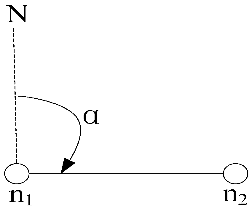
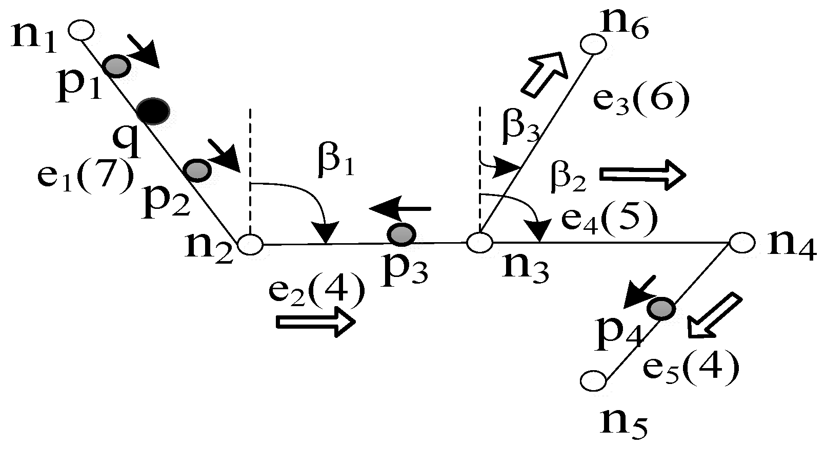
As shown in Figure 5, the horizontal angle between the reference point, which is denoted as n1, and the target directional line, which is denoted as n1n2, is α. In the road network, node is either the starting node or the ending node of edge; hence, the azimuth angle, namely, β, of the road network expansion is or . In Figure 6, if the current accessing node is n3, its extended adjacent edges are e3 and e4, the extended direction has two, when the extended edge , and the extended direction is n3 to n6, then β = β3; when the extended edge and the extended direction is n3 to n4, β = β2.
Using the direction of road network expansion, the rules for judging whether the moving object is moving on road network towards query object are as follows: when the road network extends to the adjacent edge, which is denoted as , the direction of moving object is denoted as γ, the direction of road network expansion is denoted as β. The moving object is moving towards the query object if it satisfies the inequality ε-180 ≤ γ-β≤ 180-ε (ε is the minimum deviation of the azimuth).
Based on the method for identifying the moving objects of road network that are moving towards query object, this paper uses R-tree to quickly retrieve the road edges and an INE-based road network expansion method to query the K-nearest moving objects, which efficiently identifies the K-nearest objects that are moving towards the query object. The algorithm generates a priority queue according to the distance from each network node to the query object and the priority queue controls the expansion order of the network. The closer a node is, the earlier its adjacent edges will be expanded. If an adjacent edge e of node v is currently expanding and all the moving objects on the adjacent edge have been retrieved, then use the azimuth angle to judge whether these objects are moving towards the current road network node v. If p is moving towards v, the road network distance from p to the query object is calculated, and put p into the result set. Then, the adjacent edge e is marked as “expanded” and this process will continue until there are K objects in the result set. Only when the distance from the next road network node to the query object is smaller than the distance from the farthest neighbor of the result set to the query object; otherwise, the algorithm directly returns the K objects that are moving towards the query object.
For the problem in Figure 3, since the speed of q is 1, the time to reach road network node n2 is 8; therefore, in the time interval [0, 4], q always moves on the same road edge. In this stage, we must identify the K-nearest neighbor object that is moving towards the query object at timestamp 0. Combined with the INE road network extension and the direction determination method, the algorithm process is as follows: first, edge e1 is retrieved, object p1 is acquired, p1 is moved towards the query object, and the distance between p1 and the query object is inserted into the result set: R = {(p1,6)}. Node n2 is closest to the query object and adjacent edges e2, e3, and e4 of node n2 are extended, p4 is retrieved on edge e2 and the direction of p4 is opposite the direction of expansion. Thus, R = {(p1, 6), (p4, 16)}. Next, p3 at edge e3 is retrieved, since the distance from the query object is 14, which is smaller than p4, R = {(p1, 6), (p3, 14)} is inserted; on edge e4, p6 is retrieved and it is determined that p6 is consistent with the expansion direction; the moving direction is far from the query object, and the condition is not satisfied. Then, the other end node, namely, n1 of e1, is expanded and the moving object on the adjacent edge of n1 is retrieved. The algorithm terminates when the distance of the next node of the algorithm is larger than the distance of the second-nearest-neighbor object to the query object. The final result is R = {(p1, 6), (p3, 14)}.
4.2. Evaluation of Monitoring Range in Continuous Queries
The objective of this stage is to obtain the road network monitoring range of the query request. For the time sub-interval, namely , of the query, the direction-aware road network moving object KNN query technology is used to identify the KNN object that is moving towards the query point and the result set is {p1, p2…, NNk}. In this result set, NNk is the object farthest from the query point. The monitoring distance (MD) is calculated according to the result set, and it ensures that only an object that is within the monitoring distance can become the final continuous query result. Knowing that the objects in the KNN result set are all moving towards the query point and the distance between NNk and the query point is the largest at timestamp ti. The MD is calculated as follows:
There are three parts as follows: (1) represents the distance between NNk and the query point at timestamp ; (2) represents the distance that query point q moves between ; and (3) AD represents an additional distance to ensure that all potential candidates for the KNN results are monitored in the query process within the time interval . AD is calculated as follows: firstly, the set of edges arrived after extending the distance of from the query point is determined and the additional distances of these edges are calculated as . Then, the maximum additional distance is .
If the distance from an object on an edge to a query point exceeds , but this object moves towards the query point at the maximum speed for this edge, the moving object may be the result of the continuous KNN query. Therefore, we must add an additional distance to avoid missing all possible KNN results.
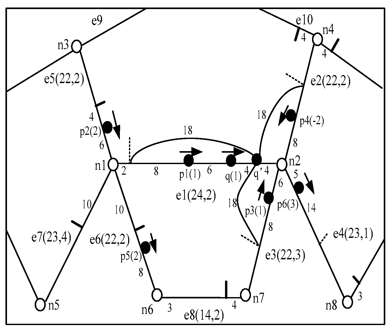
We consider the example in the previous section. After the DAKNN query processing stage, we obtain K-nearest neighbor object R = {(p1, 6), (p3, 14)}, , . The distance that q moves in time interval [0, 4] is 4 and the road network monitoring distance is MD = 14 + 4 + AD, as shown in Figure 7. The objects p1 and p3 in the result set move towards the query point; hence, the distance between p1 or p3 and query point must be less than 18 in the time interval [0, 4]. That is, at timestamp 4, the query point arrives at q’ and a distance of 18 is extended from the query point q’ and marked with dotted lines. In Figure 7, the marks fall on edges e1, e2, e3, and e4 and AD = max {2*4, 2*4, 3*4, 1*4} = 12. Therefore, the monitoring range of the road network is 30 and by expanding by a distance of 30 from query point q’, the monitoring range is obtained and marked with solid lines in Figure 7.
4.3. Identifying Candidate Objects
This stage is a process to prune the search space and gets all moving objects for which the road network distances are less than MD. The task at this stage is mainly to build a local road network and to obtain candidate objects.
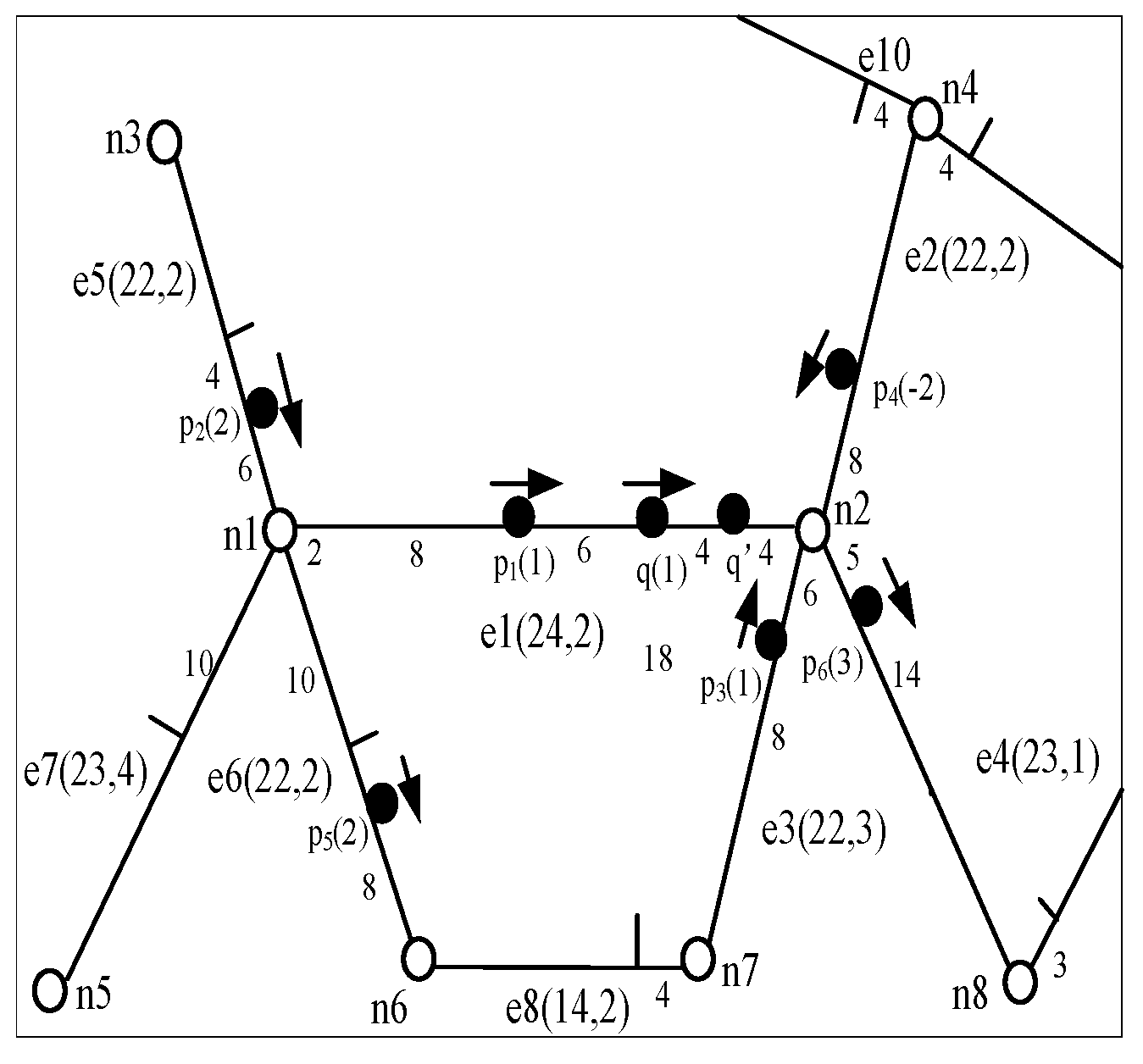
The first task is to build a local road network; all the edges in the monitoring range are added to the list of influential edges for constructing a local road network. We use the road network expansion method to expand the road network from near and far from the road edge where the query point is located. For one road edge, if the distance from one of the nodes to the query point is less than MD, add it to influence edges to participate in the construction of the local road network. It is specifically stated that the Dijkstra algorithm is used to pre-calculate the shortest distance from the nodes in the local road network to the query point. The purpose of pre-calculation is to avoid inefficiencies caused by online distance calculation. That is to say, in the subsequent calculation process of the distance from the moving point to the query point, the pre-calculation improves the efficiency of the algorithm. The information in the local road network is useful information that may affect the query result and the moving object in the local road network is also the candidate object of the query result. Our next task is to obtain the moving object moving towards the query point in the local road network as the candidate object, then use the proposed method to determine the direction of moving object. As shown in Figure 8, the final set of candidate objects is {p1, p2, p3, p4}.
4.4. Validating Candidate Objects
After the pruning stage, any object that cannot be the query result is excluded and a candidate object set, namely, {p1, p2…, pm} (m ≥ k), in the specified interval, namely [t0, tn], is obtained. Since the object is continuously moving, the query result may change within this time interval; if we cannot determine the time point at which the change occurs, queries at multiple timestamps maybe return the same query result. To reduce the cost of repeated query, we proposed the verification algorithm for determining the time points at which the time interval is divided into sub-intervals, which ensures that the query result set remains unchanged over each sub-interval.
In the verification algorithm, we first divided the specified time interval, namely, into several sub-intervals, namely, based on the time points when the candidates arrive at the nodes of the road network. When the moving objects arrive at the network nodes, the formula for calculating the distance between them and the query point will change. For each sub-interval, the distance between the moving object and the query point is determined via a specified linear function of time.
The objective of the verification algorithm is to identify the time point of the KNN result set change in each sub-interval , so that the result set is the same at any timestamp within two consecutive . Using the DAKNN method, which was introduced in Section 4.1, to obtain the query result set Q of initial time , the first object to be replaced by other candidate objects in the query result set Q must be NNk. The distance between the moving object NNk and the query point should be recorded as . For each of the candidate objects, the time point at which NNk is replaced by pi can be calculated via equation and the minimum calculated time point can be selected as the time point of change tc1. There are two cases as follows: (1) if object pi is in the KNN result set, the query result only changes in order and pi becomes a new NNk; (2) If object pi is not in the KNN result set, time subinterval is divided into and . For partitioned , the query results at any time in the subinterval are consistent with those at time . For partitioned [tc1, tm], NNk of query result Q is replaced by pi as the query result at time tc1 and the above calculation process is repeated until the time of change exceeds tm.
We proceed with the example from the previous stage to verify that we have obtained the result set of candidate objects: {p1, p2, p3, p4}. In Figure 8, we divide the time interval, namely, [0, 4], into sub-intervals according to the time when the p2 arrives at the road network node: [0, 3] and [3, 4]. First, we verify subinterval [0, 3]. At time 0, KNNs = {p1, p3} and NNk = p3. Using the equation to verify each candidate, it is concluded that object p4 replaces p3 at time 2 and p4 is not in the KNN result set; thus, the result set changes at time = 2. Therefore, time sub-interval [0, 3] is divided into [0, 2] and [2, 3] and the query results are <{p1, p3}, [0, 2]> and <{p1, p4}, [2, 3]>. For time interval [3, 4], the candidates are validated via the same processes. At time 10/3, p1 replaces p4 and p1 is in the KNN set; the final result is R= <{p1, p3}, [0, 2]>, <{p1, p4}, [2, 10/3]>, and <{p4, p1}, [10/3, 4]>.
5. Results and Analysis
This section evaluates the DACKNN query algorithm in road networks via detailed comparative test schemes. The performance of the algorithm is measured in terms of the execution time of the CPU. The results demonstrate that the proposed DACKNN method can efficiently process direction-aware continuous K-nearest neighbor queries of moving objects in road networks.
5.1. Parameter Setting
The comparative test is implemented in Java and run on an Intel (R) Core (TM) i5-6200U CPU @ 2.30 GHz processor, 4G memory, and 64-bit Windows 10 operating system. The comparative test data in this paper include road network data and moving object data, as presented in Table 1. The road network data are based on Los Angeles from TIGER/Line [28] and include 195,888 road nodes and 267,536 edges. At the same time, the Brinkoff Road Network Data Simulator [29] was used to generate moving object data with moving directions. When the moving object arrives at a road network node, it randomly selects the next path. These data objects are evenly distributed in the road network, and there are 10,000–100,000 of them.
The performance of the comparative test algorithm is mainly measured in terms of the CPU execution time. The effects of the number of moving objects, the number of K-nearest neighbors and the time interval of continuous query on the query performance are investigated via the control variable method. Because the location of the query point affects the execution time, we execute 1000 non-concurrent queries at various locations and the average execution time is taken as the comparative test result for analysis. The default settings of each parameter are adopted by the current mainstream continuous nearest neighbor queries of moving objects that are based on the road network, as listed in Table 2.
In addition, we analyzed the performances and accuracies of the CKNN, SCKNN, and DACKNN algorithms, and demonstrated the advantage of DACKNN.
5.2. Comparative Test Results and Analysis
First, the DACKNN algorithm is analyzed under various parameter settings. Second, the time efficiency and accuracy are compared with those of the SCKNN and CKNN query algorithms. Finally, the shortcomings are identified to facilitate improvement in future work. In this comparative test, default values are used for all variables unless otherwise specified.
5.2.1. Evaluation of the DACKNN Algorithm
We conduct a series of comparative tests in which we vary the number of neighbors: K, the number of moving objects and the time interval and analyze the performance of DACKNN under the parameter settings.
- (1)
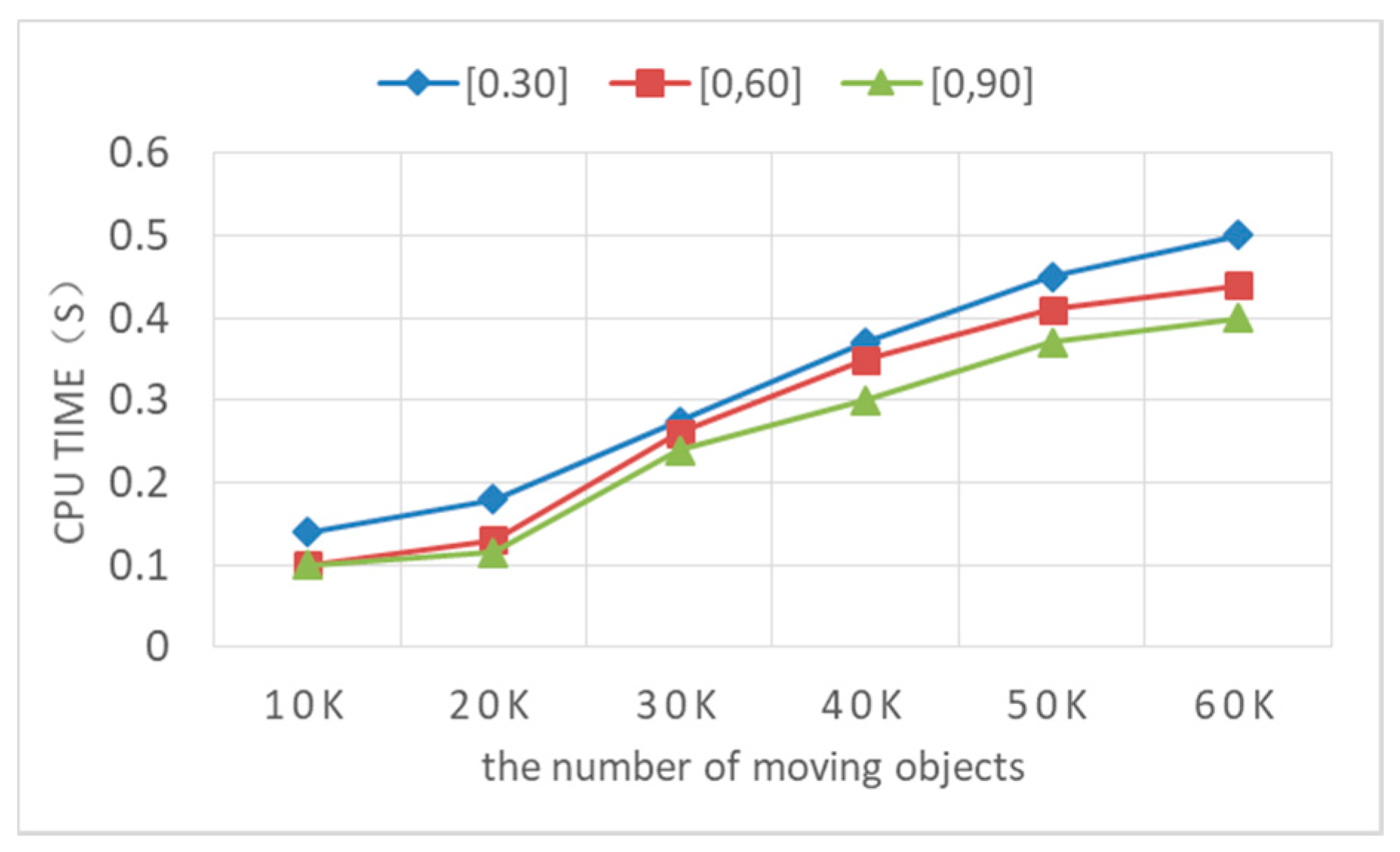
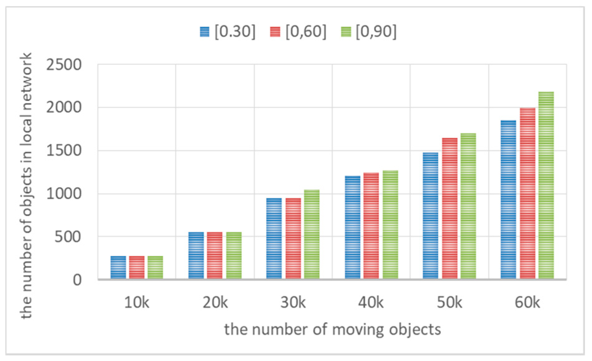
- The influence of the number of moving objects on the query performance.According to Figure 9, the value of K is 30. In the comparative tests, we compared the effects of the number of moving objects on the overall continuous query performance in three-time intervals: [0, 30], [0, 60], and [0, 90]. As shown in this Figure 9, the overall query time increased with the number of moving objects and when the number of moving objects is between 10,000 and 20,000, the query performance among the query intervals tended to be stable. This is because the number of objects in the local road network that was established by the monitoring range increased and the time cost of judging whether each moving object was moving towards the query point and executing the verification algorithm also increased. As shown in Figure 10, according to the number of moving objects in the global road network, the number of moving objects in the local road network that was established by the monitoring range of time intervals [0, 30], [0, 60], and [0, 90] is displayed. The figure shows that as the number of moving objects in the global road network increases gradually, the number of objects in the local road network also increases. The more objects there are, the longer it takes to evaluate the candidate objects. Hence, the complete algorithm becomes more time-consuming as the number of moving objects increases. From Figure 9, we also can see the larger the time interval, the higher the time cost of the algorithm. In different time intervals, when the interval difference is not very large, the calculated monitoring distances are similar and the numbers of moving objects in the local road networks that were established according to the monitoring ranges are almost the same. However, the longer the time interval is, the more time-consuming the whole algorithm will be, because the longer the time interval is, the number of moving objects that have arrived at the nodes increases, the time interval is divided into several sub-intervals according to their arrival times, and the road network distances between them and the query object are recalculated; thus, the time-consuming will increase accordingly.
- (2)
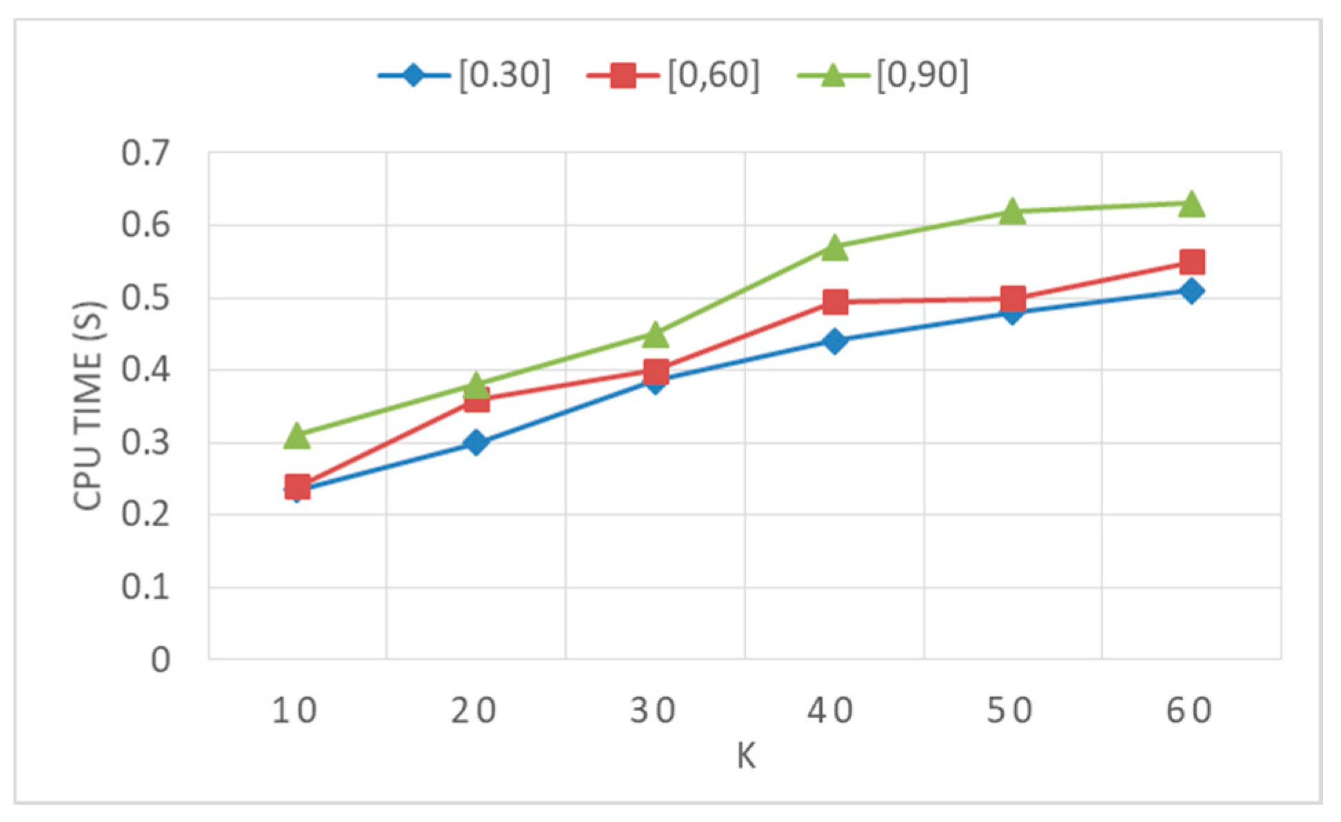
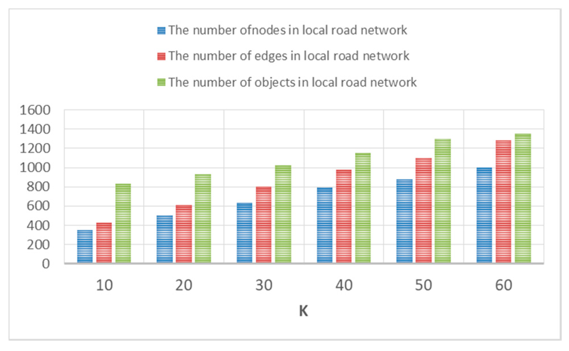
- The influence of the number of neighbors on the performance.Figure 11 shows the query execution in the Los Angles road network with 50,000 moving objects. The overall query time varies with the K under the query intervals: [0, 30], [0, 60], and [0, 90]. As shown in Figure 11, when the numbers of moving objects are the same, as K increases, the overall query running times will increase. This is because the scale of local road network gradually increases with an increase of K, thereby resulting in an increasing number of objects to be verified. Figure 12 shows how the numbers of edges, nodes and moving objects in a local road network vary with the K value. With the increase of K, the scale of local road network increases gradually and the number of moving objects in the monitoring range of the local road network also increases gradually. If the number of neighbors, namely, K, is 10, the number of moving objects in the monitoring range is 823 and the numbers of edges and nodes in the local road network are 438 and 361, respectively. When the number of neighbors, namely, K, is 30, the number of moving objects in the monitoring range is 1021 and the numbers of edges and nodes in the local road network are 812 and 641. The K value of the nearest neighbors of the query requests increases slightly and the number of local road networks increases gradually. Thus, as the scale of the road network increases steadily, the amount of data that the query algorithm must process and verify increases and the overall query time cost also increases. From Figure 11, we can also see that the larger the time interval, the higher the time cost of the algorithm. Consistent with the analysis in the previous section, the longer the time interval is, the more sub-intervals must be updated and verified.
- (3)
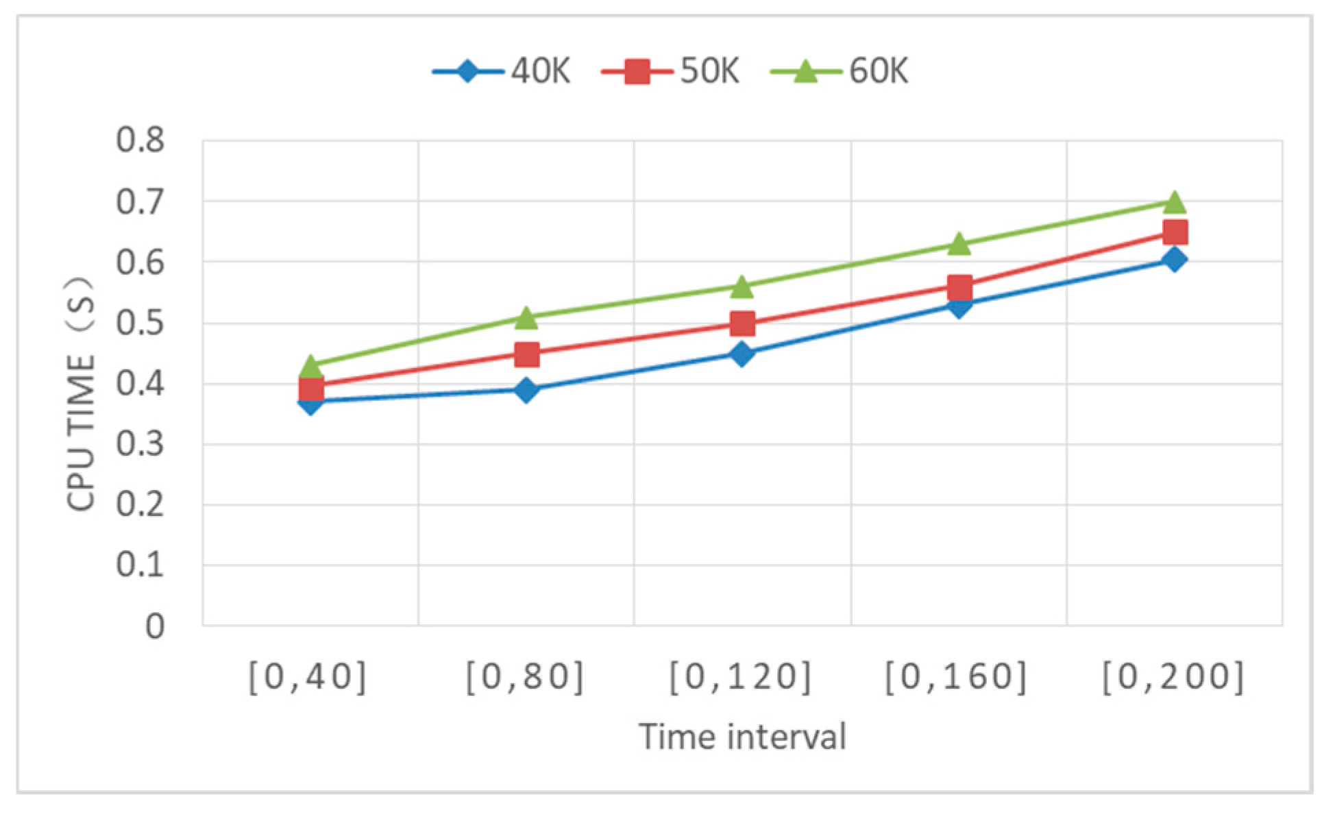
- The influence of the time interval on the overall performance.For 40,000, 50,000, and 60,000 moving objects and 30 nearest neighbors, comparative tests were carried out in various time intervals. The results are shown in Figure 13. As the length of the query time interval increases, the running time increases gradually. The larger the time interval is, the larger the monitoring range is and the larger the number of moving objects that were in the monitoring range. Moreover, with a longer time interval, more candidates arrive at the nodes of the road network in the continuous monitoring range. It is necessary to re-select the moving section, update the calculation formula for the distance from the query object, and divide the sub-intervals. These factors will lead to a higher query time cost as the time interval increases. When the moving objects are distributed in the road network with 265,536 edges, the graph shows that when the number of moving objects is small, the overall query time consumption is stable and the overall query time consumption gradually increases with the time interval. The more moving objects there are in the same time interval, the more moving objects must be retrieved and validated and the longer it takes.
- (4)
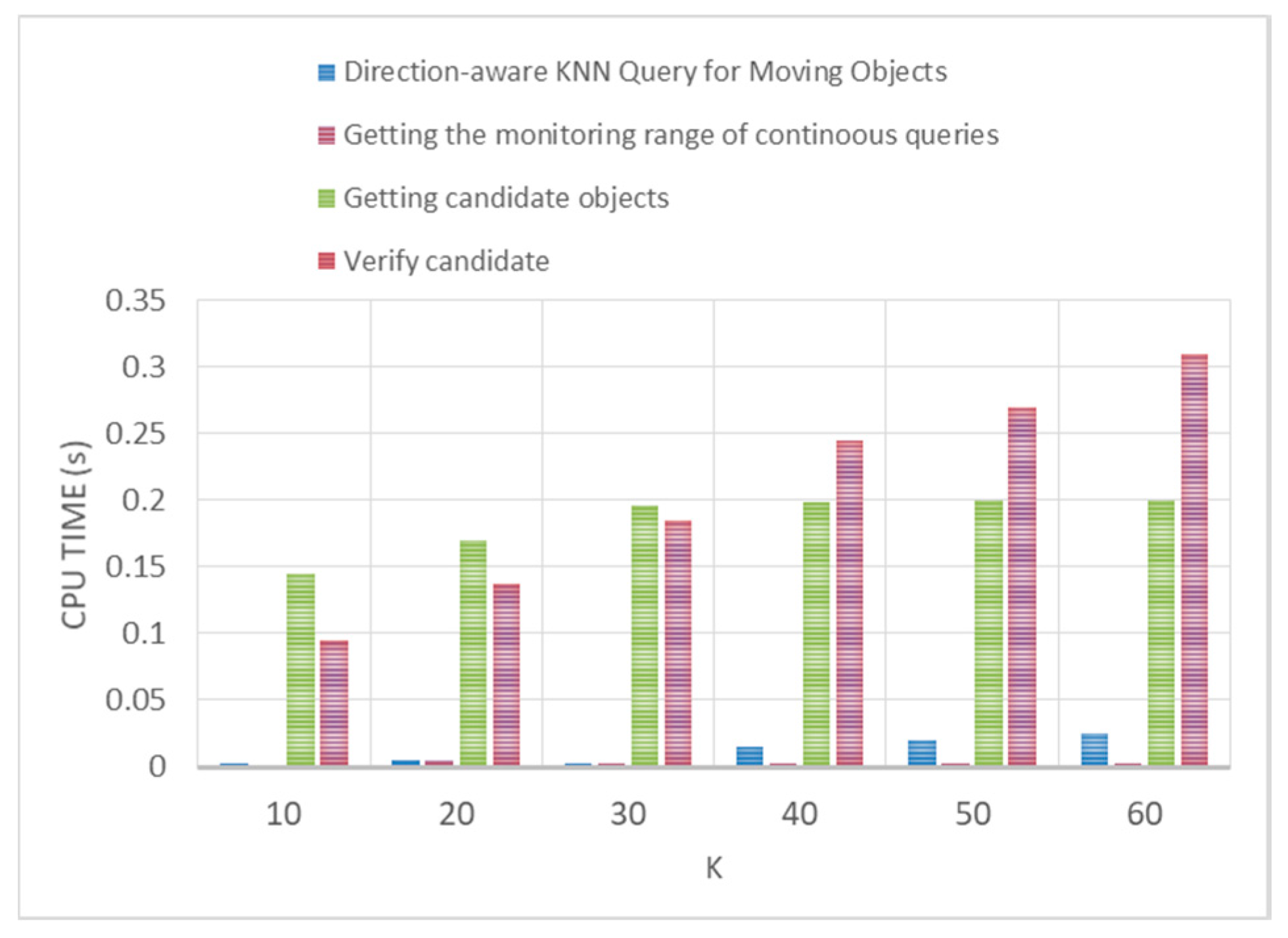
- The time-consuming situation of each stage in the algorithm.First, the comparative test makes the following comparisons according to the number of neighbors in the query: when the number of moving objects is 30,000 and the query time interval is [0, 30], the query time distribution for the K-nearest neighbors is adopted. In Figure 14, the histogram represents the time distribution of each stage of the algorithm. The first stage of the algorithm identifies the K-nearest neighbor objects that are moving towards the query point. This stage consumes a small proportion of the total time consumption of the algorithm. In the process of continuous monitoring of nearest-neighbor queries, the monitoring range is calculated by traversing the KNN result set, which costs little time. The time consumption of the stage of identifying candidate objects via road network expansion accounts for the majority of the total time consumption of the process. In this stage, the local road network is constructed according to the monitoring range and the moving objects in the local road network are evaluated. In the process of identifying the moving objects, according to the diagram, the time-consumption occupancy ratio is the highest out of the whole process when the number of K-nearest neighbors is small. In the process of validating the candidate objects, the time interval is divided into several sub-intervals according to the arrival timestamps of the candidate objects at the node of the road network and a result set is obtained in each sub-interval. When dividing the time interval, it is necessary to update each object that arrives at the node and to recalculate the road network distance to the query point. The more candidate objects and K-nearest neighbors, the higher the time consumption of the validation process; the time consumption of the verification stage will also increase.
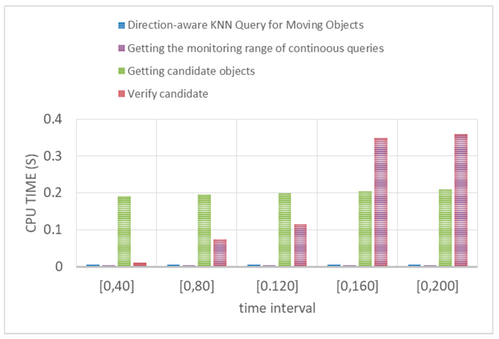
Then, the comparative test makes the following comparisons according to the various query time intervals. When the number of moving objects is 30,000 and the number of neighbors, namely, K, is 10, the time distribution of each stage of the algorithm is observed for various query time intervals: [0, 20], [0, 40], [0, 60], [0, 80], and [0, 100]. In Figure 15, the histogram shows the time distribution of each stage of the algorithm and the time-consumption trend is stable for acquiring direction-aware neighbors and monitoring ranges. When the number of K-nearest neighbors is constant, the time-consumptions of the K-nearest neighbor queries that are acquired at the starting time are stable when the starting times are the same. In the whole process, it is time-consuming to obtain and verify candidate objects. In the stage of obtaining candidate objects, the influential edges are identified according to the monitoring range, a local road network is created, and the moving objects in the local road network are retrieved as candidate objects. With the increase of the time interval, the monitoring range becomes larger and the amount of data that must be processed increases. The time-consumption of the candidate validation stage increases with the time interval. The longer the time interval is, the larger the monitoring range is, the more edges that must be retrieved, and the larger the number of candidates that must be evaluated. Moreover, the longer the time interval is, the larger the number sub-intervals into which it must be divided. For each sub-interval, the candidates must be evaluated; thus, the time-consumption increases with the number of sub-intervals.
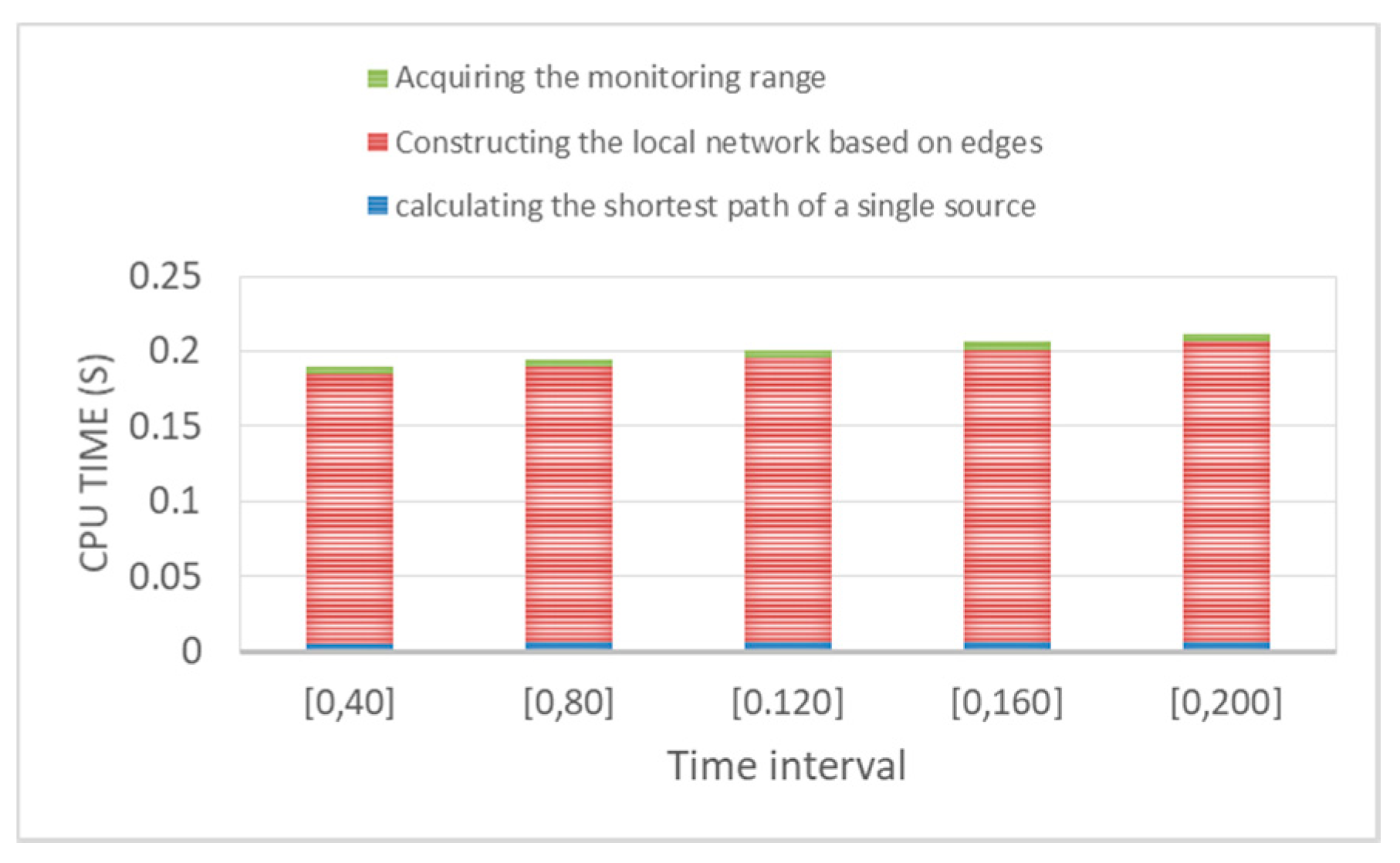
To deal with the continuous K-nearest-neighbor query and improve the query efficiency, we must transform the global network into a small-scale local network to facilitate the retrieval of objects. We analyze the time-consumption of the whole process of constructing the local network. As shown in Figure 16, in the process of local road network construction, the time consumption of determining the monitoring range is very small. According to the size of the monitoring range, the query point-centered edge is acquired and the local road network is constructed on the edge of the monitoring range; this process is time-consuming. As the time interval increases, the monitoring range increases and the acquisition influence edge becomes larger, thereby increasing the processing time. The time consumption for calculating the shortest path of a single source on a local road network is negligible.
5.2.2. Comparison with Other Algorithms
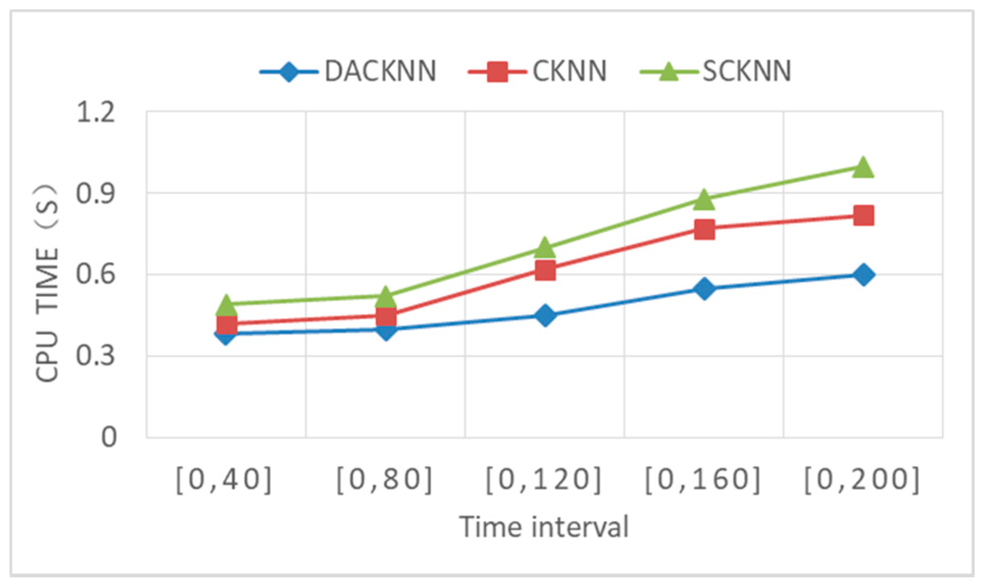
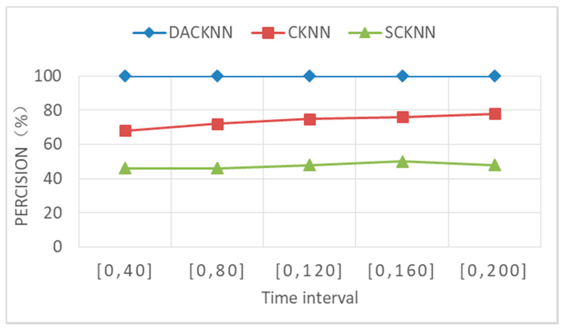
First, we evaluate the effects of the CKNN, SCKNN, and DACKNN algorithms on the time consumption as the time interval increases and their accuracies. Here, accuracy refers to the accuracy with which moving objects that are moving towards the query point are identified, which is expressed as a percentage. According to Figure 17, the time costs of these three algorithms increase with the time interval because more moving objects will arrive at the network nodes over a larger time interval; thus, the time interval is divided into more sub-time intervals for verification. However, the time costs of CKNN and SKNN increase faster as the time interval increases because these two algorithms do not screen out objects that are moving towards the query object, but consider all objects in the monitoring range as candidates; thus, the more objects they deal with, the more time they consume. The DACKNN algorithm can filter out objects that are moving away from the query point in the monitoring range. Thus, the number of candidate objects is smaller; therefore, DACKNN outperforms SCKNN and CKNN in terms of time consumption. Figure 18 shows the accuracies of these three algorithms. The moving objects that are moving towards the query object can be obtained with 100% accuracy by the DACKNN algorithm as the time interval increases, while the accuracy of SCKNN reaches more than 70%, and the accuracy of CKNN is approximately 50%.
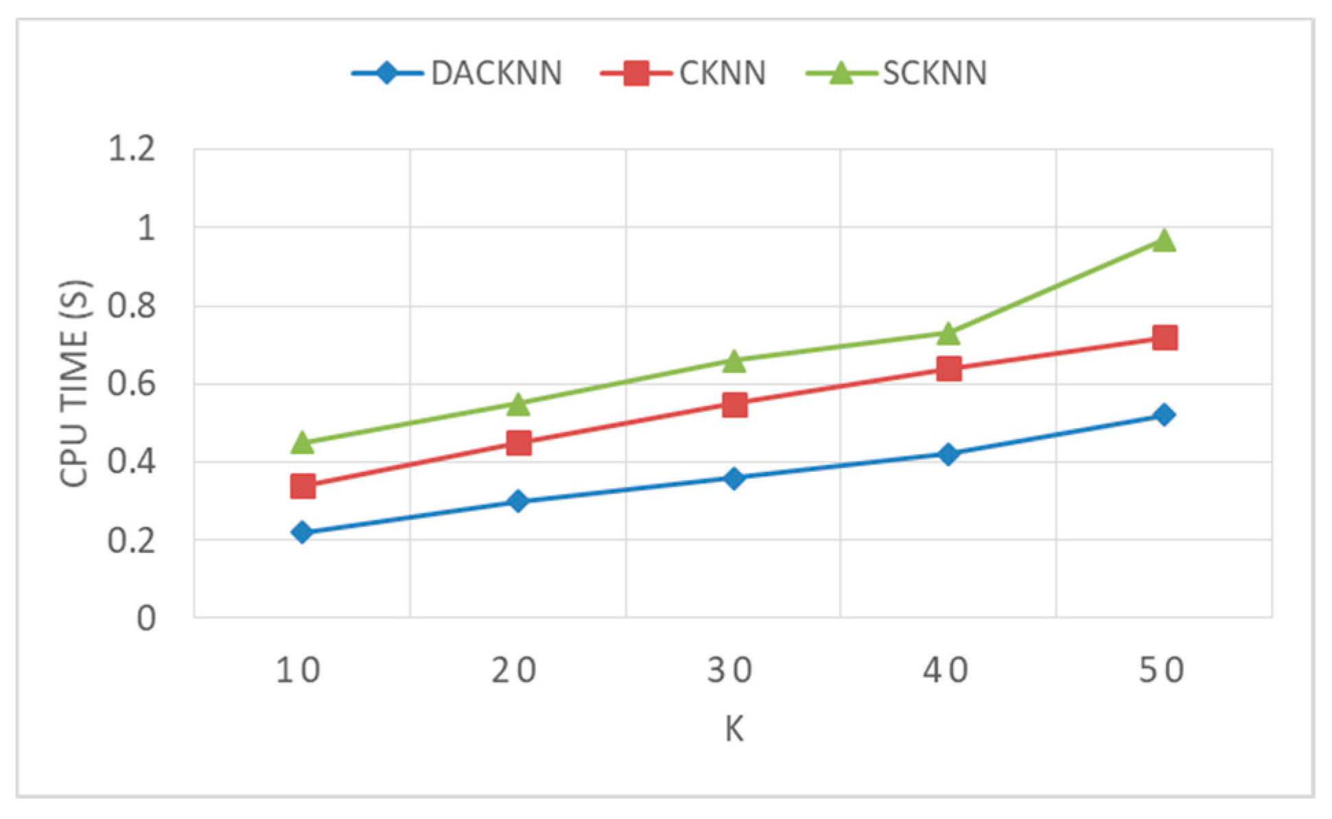
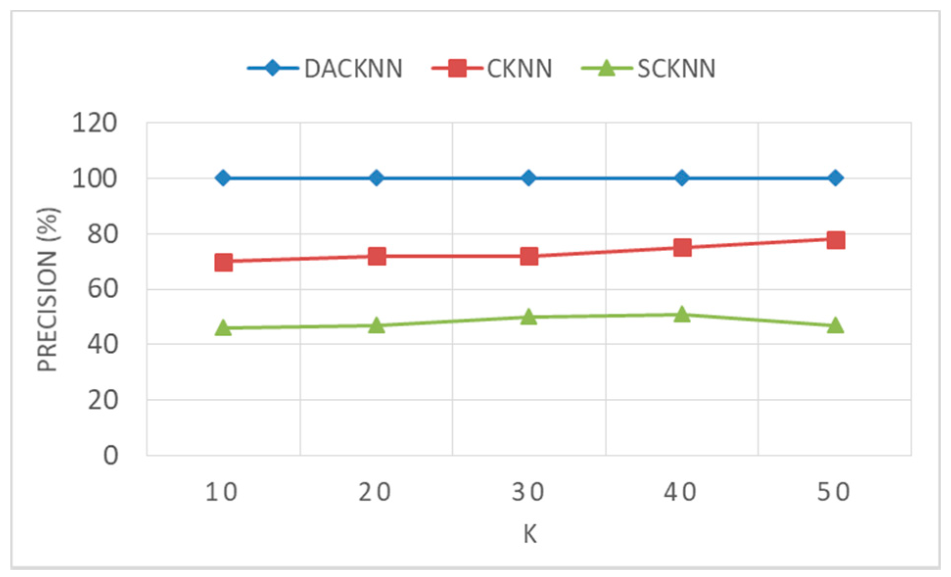
Figure 19 shows that the time costs of CKNN, SCKNN and DACKNN will increase as the value of K increases. This is because with the increase of K, a larger monitoring range is needed to ensure that there are K objects in this range, and more candidate objects are needed to verify. The overall time consumption of the proposed DACKNN algorithm is lower than those of other two query algorithms, and its overall performance is higher than CKNN and SKNN. Figure 20 shows the accuracy of three algorithms with the increase of K. It can be seen that the moving objects towards query object can always be obtained 100% by DACKNN algorithm as K increases, while the accuracy of moving objects obtained by SCKNN algorithm is between 60% and 80%, and the accuracy of CKNN algorithm is nearly 50%.
The results show that the proposed DACKNN algorithm is superior to SCKNN and CKNN. By utilizing the directional characteristics of moving objects, the DACKNN determine moving objects moving towards query point, and filters out some objects far from the query point in the monitoring range, thus improving the overall performance and effectiveness of the query algorithm.
6. Conclusions
This paper presents a direction-aware continuous moving K-nearest-neighbor query algorithm in road networks. In this algorithm, we adopt an efficient direction determination method that is based on road network expansion to quickly judge whether moving objects are moving towards the query point. This method can filter out moving objects that are far away from the query point and reduce the number of candidate objects for continuous K-nearest-neighbor query, thereby improving algorithm efficiency. In this paper, we define the road network distance of a moving object from the query object as a function of time, so we can determines when candidate objects replace the objects in the result set. The algorithm guarantees the consistency of the query results within each sub-interval; hence, it does not make continuous query requests on continuous K-nearest neighbor queries, avoids repeated queries and reduces computational costs.
This paper initially solves the problem of direction-aware continuous moving K-nearest neighbor query in road networks. However, there are still some limitations in our method. On the one hand, due to the simulated moving objects information, the more moving objects there are, the more points will move outside the edge, and the information of each moving point that arrives at the specified node will be recorded in memory, which may lead to memory overflow of computers and cause substantial difficulties in the process of comparative tests. On the other hand, when the moving object reaches a road network node, an adjacent edge of the node is randomly selected as its next traveling edge; the moving object will travel along the selected edge. This randomness does not match the reality. In future research, we will study the processing of the node and the variable motion speed of moving objects to be more realistic.
Author Contributions
Conceptualization, T.D., Y.S. and L.Y.; Methodology, Y.S. and L.Y.; Original draft preparation, Y.Y. and Y.S.; Paper writing Y.S. and L.Y.; Data quality check, Y.S. and L.Y.; Data validation, L.Z.; Paper revision, T.D. and L.Y.; Writing-revision &editing, Y.S. and L.Y.; Project Administration, T.D.
Funding
This research was supported by the following foundations: National Natural Science Foundation of China (No.61672464, No.61572437).
Conflicts of Interest
The authors declare no conflict of interest.
References
- Tao, Y.; Papadias, D.; Shen, Q. Continuous nearest neighbor search. In Proceedings of the 28th international conference on Very Large Data Bases, Hong Kong, China, 20–23 August 2002; pp. 287–298. [Google Scholar]
- Cho, H.J.; Chung, C.W. An Efficient and Scalable Approach to CNN Queries in a Road Network. In Proceedings of the International Conference on Very Large Data Bases, Trondheim, Norway, 30 August–2 September 2005; pp. 865–876. [Google Scholar]
- Kolahdouzan, M.R.; Shahabi, C. Continuous K nearest neighbor queries in spatial network databases. In Proceedings of the STDBM, Toronto, ON, Canada, 30 August 2004; pp. 44–50. [Google Scholar]
- Liu, X.; Shekhar, S.; Chawla, S. Object-based directional query processing in spatial databases. IEEE Trans. Knowl. Data Eng. 2003, 15, 295–304. [Google Scholar]
- Patroumpas, K.; Sellis, T. Monitoring Orientation of Moving Objects around Focal Points. In Proceedings of the Symposium on Large Spatial Databases, Aalborg, Denmark, 8–10 July 2009; pp. 228–246. [Google Scholar]
- Nutanong, S.; Tanin, E.; Zhang, R. Visible nearest neighbor queries. In Proceedings of the DASFAA, Bangkok, Thailand, 9–12 April 2007; pp. 876–883. [Google Scholar]
- Papadias, D.; Zhang, J.; Mamoulis, N.; Tao, Y. Query processing in spatial network databases. In Proceedings of the Very Large Data Bases, Berlin, Germany, 9–12 September 2003; pp. 802–813. [Google Scholar]
- Ahuja, R.K.; Mehlhorn, K.; Orlin, J.B.; Tarjan, R.E. Faster algorithms for the shortest path problem. J. ACM 1990, 37, 213–223. [Google Scholar] [CrossRef] [Green Version]
- Kolahdouzan, M.R.; Shahabi, C. Voronoi-based k nearest neighbor search for spatial network databases. In Proceedings of the Thirtieth International Conference on Very Large Data Bases, Toronto, ON, Canada, 31 August—3 September 2004; Volume 30. [Google Scholar]
- Hu, H.; Lee, D.L.; Xu, J. Fast nearest neighbor search on road networks. In Proceedings of the Extending Database Technology, Munich, Germany, 26–31 March 2006; pp. 186–203. [Google Scholar]
- Hu, H.; Lee, D.L.; Lee, V.C. Distance indexing on road networks. In Proceedings of the Very Large Data Bases, Seoul, Korea, 12–15 September 2006; pp. 894–905. [Google Scholar]
- Lee, K.C.K.; Lee, W.C.; Zheng, B. Fast object search on road networks. In Proceedings of the International Conference on Extending Database Technology, Saint Petersburg, Russia, 23–27 March 2009; pp. 1018–1029. [Google Scholar]
- Shahabi, C.; Kolahdouzan, M.R.; Sharifzadeh, M. A road network embedding technique for K-nearest neighbor search in moving object databases. GeoInformatica 2003, 7, 255–273. [Google Scholar] [CrossRef]
- Mouratidis, K.; Yiu, M.; Papadias, D.; Mamoulis, N. Continuous nearest neighbor monitoring in road networks. In Proceedings of the VLDB, Seoul, Korea, 12–15 September 2006; pp. 43–54. [Google Scholar]
- Demiryurek, U.; Banaei-Kashani, F.; Shahabi, C. Efficient Continuous Nearest Neighbor Query in Spatial Networks Using Euclidean Restriction. In Proceedings of the International Symposium on Spatial and Temporal Databases, Aalborg, Denmark, 8–10 July 2009. [Google Scholar]
- Huang, Y.K.; Chen, Z.W.; Lee, C. Continuous K-Nearest Neighbor Query over Moving Objects in Road Networks. In Advances in Data and Web Management; Springer: Berlin/Heidelberg, Germany, 2009; pp. 27–38. [Google Scholar]
- Li, G.; Fan, P.; Li, Y.; Du, J. An Efficient Technique for Continuous K-Nearest Neighbor Query Processing on Moving Objects in a Road Network. In Proceedings of the Computer and Information Technology, 29 June–1 July 2010; pp. 627–634. [Google Scholar]
- Gao, Y.; Zheng, B.; Lee, W.C.; Chen, G. Continuous visible nearest neighbor queries. In Proceedings of the EDBT, Saint Petersburg, Russia, 24–26 March 2009; pp. 144–155. [Google Scholar]
- Li, G.; Feng, J.; Xu, J. Desks: Direction-aware spatial keyword search. In Proceedings of the IEEE 28th International Conference on Data Engineering (ICDE), Arlington, VA, USA, 1–5 April 2012; pp. 474–485. [Google Scholar]
- Yi, S.; Ryu, H.; Son, J.; Chung, Y.D. View field nearest neighbor: A novel type of spatial queries. Inf. Sci. 2014, 275, 68–82. [Google Scholar] [CrossRef]
- Lee, K.C.K.; Lee, W.C.; Leong, H.V. Nearest surrounder queries. In Proceedings of the ICDE, Atlanta, GA, USA, 3–8 April 2006; p. 85. [Google Scholar]
- Lee, K.C.K.; Schiffman, J.; Zheng, B.; Lee, W.-C.; Leong, H.V. Tracking nearest surrounders in moving object environments. In Proceedings of the ICPS, Lyon, France, 26–29 June 2006; pp. 3–12. [Google Scholar]
- Lee, K.C.K.; Schiffman, J.; Zheng, B.; Lee, W.-C.; Leong, H.V. Roundeye: A system for tracking nearest surrounders in moving object environments. J. Syst. Softw. 2007, 80, 2063–2076. [Google Scholar] [CrossRef]
- Guo, X.; Zheng, B.; Ishikawa, Y.; Gao, Y. Direction-based surrounder queries for moving recommendations. VLDB J. 2001, 20, 743–766. [Google Scholar] [CrossRef]
- Lee, M.J.; Choi, D.W.; Kim, S.; Park, H.M.; Choi, S.; Chung, C.W. The direction-constrained k nearest neighbor query. GeoInformatica 2016, 20, 471–502. [Google Scholar] [CrossRef]
- Chen, Z.; Shen, H.T.; Zhou, X.; Yu, J.X. Monitoring path nearestneighbor in road networks. In Proceedings of the SIGMOD, Providence, RI, USA, 29 June–2 July 2009; pp. 591–602. [Google Scholar]
- Tianyang, D.; Lulu, Y.; Qiang, C.; Bin, C.; Jing, F. Direction-aware KNN queries for moving objects in a road network. World Wide Web 2019, 22, 1765–1797. [Google Scholar] [CrossRef]
- U.S. Census Bureau. TIGER/Line Shapefiles. 2013. Available online: http://www.census.gov/geo/www/tiger (accessed on 1 September 2013).
- Brinkhoff, T. A framework for generating network-based moving objects. GeoInformatica 2002, 6, 153–180. [Google Scholar] [CrossRef]
Figure 1.
The local road network information under different timestamp: (a) at timestamp 0; (b) at timestamp 2.
Figure 1.
The local road network information under different timestamp: (a) at timestamp 0; (b) at timestamp 2.

Figure 2.
The local road network information.

Figure 3.
Road network at timestamp 0.

Figure 4.
Direction-aware continuous moving K-nearest neighbor (DACKNN) algorithm process diagram.

Figure 5.
Azimuth angle.

Figure 6.
Azimuth angle of road network expansion.

Figure 7.
An example of monitoring range.

Figure 8.
The Local Road Network.

Figure 9.
Comparisons of time consumed with the number of moving objects in different time intervals.
Figure 9.
Comparisons of time consumed with the number of moving objects in different time intervals.

Figure 10.
The number of objects in local road networks varies with the number of moving objects in different time intervals.
Figure 10.
The number of objects in local road networks varies with the number of moving objects in different time intervals.

Figure 11.
Effect of K value on Performance.

Figure 12.
The number of nodes, edges, and moving objects in local road network with different K values.
Figure 12.
The number of nodes, edges, and moving objects in local road network with different K values.

Figure 13.
Effect of different time intervals on performance.

Figure 14.
Time-consuming for each stage of continuous query for different K values.

Figure 15.
Time-consuming for each stage of continuous query in different time intervals.

Figure 16.
Time-consuming of local road network construction stage under different time interval.

Figure 17.
Time consumption of algorithms under different time intervals.

Figure 18.
Accuracy of algorithms under different time intervals.

Figure 19.
Time consumption of Algorithms for different K values.

Figure 20.
Accuracy of Algorithms for different K values.


Table 1.
Comparative test data.
| Parameters | Values |
|---|---|
| Los Angeles Edge | 267,536 |
| Los Angeles Node | 195,888 |
| Moving object | 10K~100K |
| K | 1~100 |
| Time interval t | 0~100 |
Table 2.
Default parameter settings for comparative tests.
| Parameters | Default Values |
|---|---|
| R-tree maximum capacity of nodes | 50 |
| R-tree minimum capacity of nodes | 20 |
| Moving object p | 50k |
| K | 30 |
| Time interval t | 30 |
© 2019 by the authors. Licensee MDPI, Basel, Switzerland. This article is an open access article distributed under the terms and conditions of the Creative Commons Attribution (CC BY) license (http://creativecommons.org/licenses/by/4.0/).
Share and Cite
MDPI and ACS Style
Dong, T.; Yuan, L.; Shang, Y.; Ye, Y.; Zhang, L. Direction-Aware Continuous Moving K-Nearest-Neighbor Query in Road Networks. ISPRS Int. J. Geo-Inf. 2019, 8, 379. https://doi.org/10.3390/ijgi8090379
AMA Style
Dong T, Yuan L, Shang Y, Ye Y, Zhang L. Direction-Aware Continuous Moving K-Nearest-Neighbor Query in Road Networks. ISPRS International Journal of Geo-Information. 2019; 8(9):379. https://doi.org/10.3390/ijgi8090379
Chicago/Turabian StyleDong, Tianyang, Lulu Yuan, Yuehui Shang, Yang Ye, and Ling Zhang. 2019. "Direction-Aware Continuous Moving K-Nearest-Neighbor Query in Road Networks" ISPRS International Journal of Geo-Information 8, no. 9: 379. https://doi.org/10.3390/ijgi8090379
Note that from the first issue of 2016, this journal uses article numbers instead of page numbers. See further details here.