Transition Models for Turbomachinery Boundary Layer Flows: A Review

Abstract

Current models for transition in turbomachinery boundary layer flows are reviewed. The basic physical mechanisms of transition processes and the way these processes are expressed by model ingredients are discussed. The fundamentals of models are described as far as possible, with a common structure of the equations and with emphasis on the similarities between the models. Tests of models reported in the literature are summarized and our own test is added. A conclusion on the performance of models is formulated.

1. Transition Mechanisms

With the objective of modelling with Reynolds-averaged Navier-Stokes (RANS) or URANS (unsteady or time-accurate RANS) description of a flow, generally, four types of transition from laminar state to turbulent state in turbomachinery boundary layer flows are distinguished [1,2]. These are: natural transition in attached boundary layer state, bypass transition in attached boundary layer state under a statistically steady mean flow, separation-induced transition in the free shear layer formed by separation of a boundary layer under a statistically steady mean flow, and wake-induced transition due to periodically unsteady impact of wakes on boundary layers in attached or separated state. Despite the vast amount of studies on these transition types during the last 4 or 5 decades, understanding of the mechanisms is still not complete, although large progress has been made in the last decade thanks to direct numerical simulation (DNS) and large-eddy simulation (LES). Hereafter, we summarise the mean mechanisms, taking into account the inherent limitations of modelling with Reynolds-averaged Navier-Stokes description of a flow. This means that secondary effects, which mostly are the least understood and sometimes still are a matter of controversy, are not discussed, because, anyhow these features cannot be represented by RANS or URANS.

1.1. Natural Transition

Under a statistically steady mean flow of low turbulence level, transition in an attached boundary layer is initiated by 2D viscosity-dependent Tollmien-Schlichting instability waves, followed by a 3D instability, leading to formation of spanwise periodic hairpin vortices, which, farther downstream, cause breakdown of the laminar layer with generation of turbulent spots. These spots finally merge resulting in the formation of a turbulent boundary layer [1,2]. This type of transition is called natural transition. It is a rather slow process and, under a very low mean-flow turbulence level, as in external aerodynamics, it is very sensitive to all sorts of perturbations. This makes the prediction of transition in external aerodynamics very delicate. However, in turbomachinery flows, the mean-flow turbulence level is never extremely low and turbulent fluctuations perturbing the pre-transitional boundary layer amplify and control the Tollmien-Schlichting wave growth. This makes the transition process much less sensitive to other kinds of perturbations and much more amenable to simple descriptions by correlations or characteristic sensor numbers, as we will discuss in later sections.

1.2. Bypass Transition

Under a sufficiently high level of mean-flow turbulence, generally above 0.5%–1%, streamwise elongated disturbances are induced in the near-wall zone of an attached laminar boundary layer, termed streaks or Klebanoff distortions. They are zones of forward and backward jet-like perturbations, alternating in spanwise direction with almost perfect periodicity, with a wavelength in the order of the boundary layer thickness. The streaks are caused by deep penetration of low-frequency disturbances, while high-frequency disturbances are strongly damped by the laminar shear layer. This damping is called shear-sheltering. The laminar boundary layer distorted by the streaks is susceptible to instabilities. A remarkable feature is that the streak patterns are of large wavelength, but that the instability patterns are of short wavelength. This means that the instability patterns can only be excited by high-frequency perturbations, although these are damped by the boundary layer shear. The Klebanoff distortions grow downstream both in length and amplitude and finally cause breakdown with formation of turbulent spots. The transition is then called of bypass type, which means that the instability mechanism of the Tollmien-Schlichting waves is bypassed. Flow breakdown is then much faster. Details of the bypass transition mechanisms were obtained by DNS and LES of many researchers [3,4,5,6,7,8,9]. There are at least two instability modes, one called outer mode or sinuous mode and one called inner mode or varicose mode. Both are a consequence of inflectional velocity profiles in wall-normal direction caused by the streaks. However, for modelling with RANS or URANS description of a flow, the details of the instabilities are not relevant.

1.3. Separation-Induced Transition

In a boundary layer with laminar separation and low or moderate mean-flow turbulence, transition is initiated by inviscid Kelvin-Helmholtz instability of the laminar free shear layer, with generation of spanwise vortices. They group at selective streamwise wavelengths, analogous to Tollmien-Schlichting waves in an attached boundary layer. The roll-up vortices become unstable by spanwise perturbations and cause breakdown as they convect downstream. This is a slow process that is sensitive to all sorts of disturbances under very low mean-flow turbulence. As with natural transition, mean-flow turbulence accelerates and controls the growth of the Kelvin-Helmholtz vortices and makes the process less sensitive to other disturbances. The mechanisms of separation-induced transition were studied by experiments, by LES and by DNS by many researchers [10,11,12,13,14,15,16,17,18,19,20,21,22,23,24]. Generally, the free shear layer, once sufficiently turbulent, reattaches forming a separation bubble. For this result, transition into turbulence does not have to be complete at the reattachment point. Under a low or moderate mean-flow turbulence level, natural transition upstream of the separation point by Tollmien-Schlichting waves can co-exist with the Kelvin-Helmholtz vortices in the separated layer. Similarly, under a higher mean-flow turbulence level, bypass transition with the formation of streaks in the pre-transitional attached boundary layer can co-exist with the Kelvin-Helmholtz vortices. The breakdown of the vortex rolls is then accelerated by the perturbation due to the Klebanoff distortions. For sufficiently strong mean-flow turbulence, the Kelvin-Helmholtz instability may even be bypassed by the breakdown due to streaks. So, a bypass mechanism is possible, similarly as in an attached boundary layer.

1.4. Wake-Induced Transition

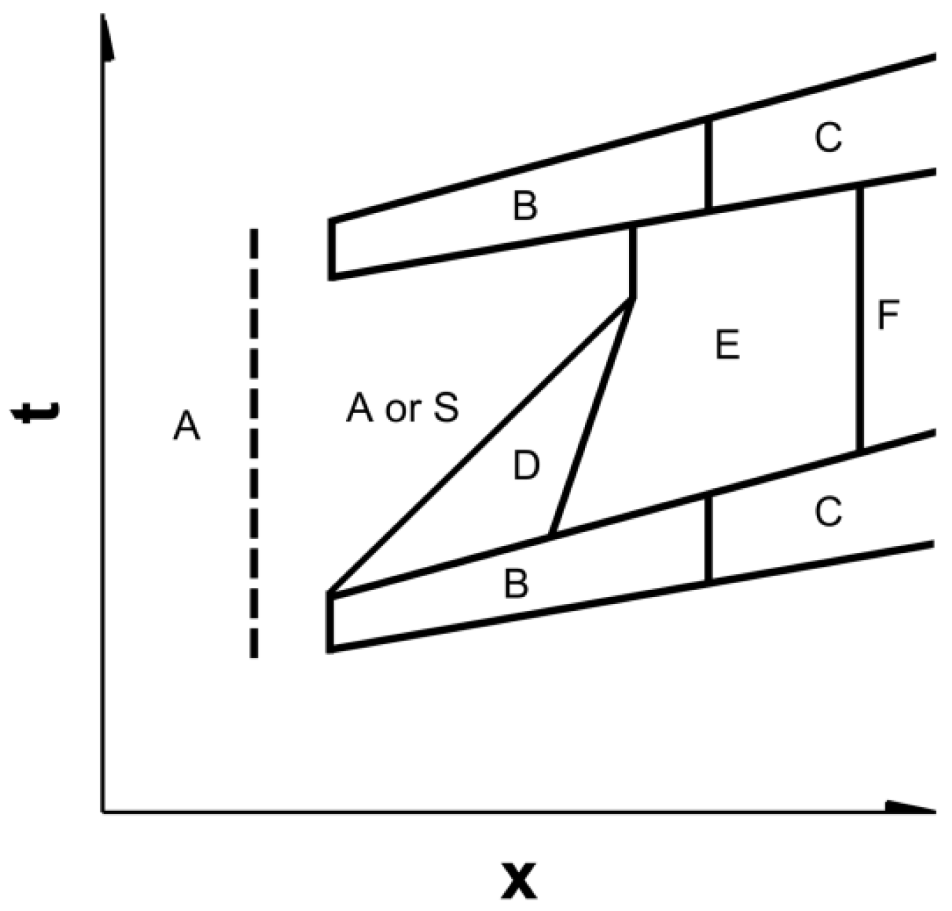
In turbomachinery flows, the transition is strongly determined by impinging wakes generated by preceding blade rows. With an attached boundary layer, bypass transition occurs under the wake path. With low or moderate kinematic perturbation by the impinging wakes, the induction of Klebanoff distortions is similar as with mean steady flow, as observed experimentally by, e.g., Liu and Rodi [25] and by Orth [26]. A general description of the transition under wake paths and in between wake paths was given by Halstead et al. [27,28,29,30] for axial turbomachines, based on tests covering a broad range of Reynolds numbers and loading levels, but always with a sufficiently high level of background turbulence such that natural transition did not occur. Figure 1 is a schematic of the different zones in a time-space diagram (t = time; x = streamwise distance along the blade surface). Along a path under wakes, the boundary layer starts in laminar state (A); undergoes transition (B) and becomes fully turbulent (C) with an evolution that is similar as under a steady free flow. For attached flow, this can be derived from the propagation speed of turbulent parts in hot-film signals, which are around 90% and 50% of free-stream velocity for leading and trailing boundaries of these parts. These velocities correspond to the propagation velocities of leading and trailing parts of a turbulent spot in a boundary layer under a statistically steady mean flow. That transitional strips lag with respect to wake trajectories was further demonstrated by Schobeiri et al. [31] for unsteady wake passages from cylindrical rods along the concave surface of a curved plate. This means that the path BC in Figure 1 is not exactly under the wake path and that its propagation speed is about 70% of the free-stream velocity. For a path in between wakes (parts E and F), the evolution is similar as under wakes, but with a later onset and completion of transition. After passage of a wake, the transitional boundary relaxes towards a laminar state, but, at start of this relaxation, the velocity profile stays close to the turbulent one, while turbulence decays very rapidly. This phenomenon is called calming of the boundary layer. The consequence is increased resistance against transition by the turbulence in between wakes (region D). The propagation speed of the trailing edge of this zone is about 30% of the free-stream velocity. Figure 1 is a schematic and the extensions of the indicated zones depend in reality on Reynolds number, free-stream turbulence level and pressure gradient. For lower Reynolds numbers, the boundary layer may separate in laminar state, but for sufficiently high free-stream turbulence level, there is reattachment. A separation zone (S) may then precede the transitional zones B and E in Figure 1. The calmed region D is then also a zone of increased resistance against separation. That the transition evolution with a separated boundary layer, for paths under wakes and in between wakes, can be similar to the evolution under a statistically steady mean flow was further demonstrated by Schobeiri et al. [32,33] for unsteady wake passages from cylindrical rods along the suction side of a low-pressure turbine profile. Turbulent spots generated by the wake impact suppress or reduce periodically the size and height of the separation bubble.

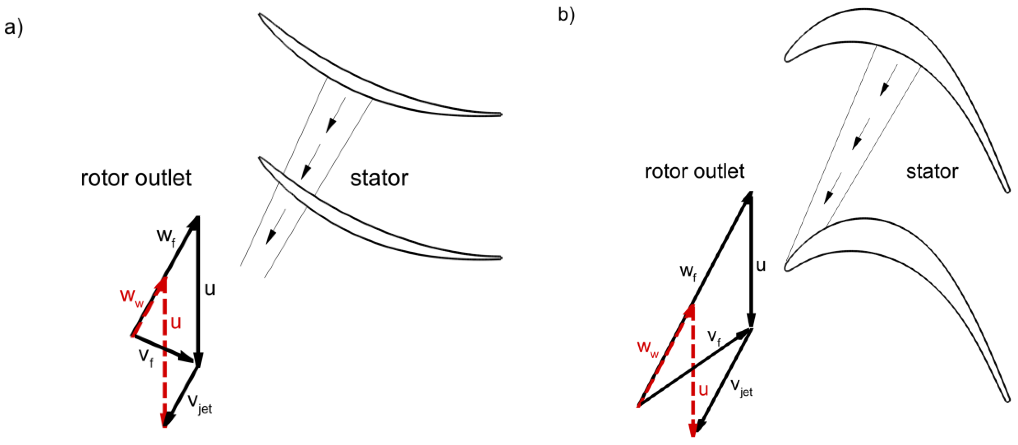
When the kinematic impact of wakes on the boundary layer is strong, the transition processes may be altered. This applies mainly to the suction side of turbine blades. Figure 2a is a schematic of the wake generated by a moving compressor rotor blade impacting on downstream stator vanes. The sketch shows that the wake results in a jet oriented towards the pressure side of a vane. This jet is commonly called a negative jet. The jet is oriented away from the suction side. The sketch also shows the jet generated by the wake of a moving turbine rotor blade on downstream stator vanes (Figure 2b). For a turbine, the negative jet is oriented towards the suction side and is oriented away from the pressure side.

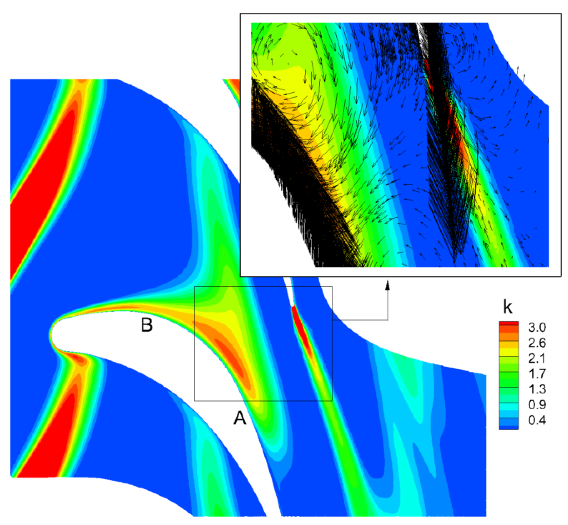
Figure 3 shows the convection of the wake turbulence and the perturbation vectors of a negative jet (instantaneous velocity minus time-averaged velocity) generated by upstream moving rods on the suction and pressure sides of a high-pressure turbine vane, used as test case later in this paper. On the suction side, the leading part of the jet causes acceleration in the boundary layer, which goes together with decreased pressure. The pressure is the highest in the centre of the jet. The boundary layer thus experiences a transient adverse pressure gradient in the leading edge zone of the jet. This may cause local flow reversal at the edge of an attached boundary layer, as demonstrated by DNS by Wu et al. [34]. If the impact of the wakes is sufficiently strong, local Kelvin-Helmholtz instability occurs in the outer part of the attached boundary layer, leading to a much faster breakdown than with bypass transition under a mean steady flow.

A particular aspect of the impacting negative jet on the suction side of a turbine blade is that, the turbulence lags the kinematic perturbation. This is visible on Figure 3. The letter A in the figure denotes the leading edge of the wake, and the letter B the turbulence in the tail of the wake. The lag comes from the deformation of the wake by the acceleration and strong curvature in the leading edge zone of the suction side. The effect of the kinematic impact lagged by the turbulence impact on the separated boundary layer on the suction side of a low-pressure turbine blade was studied by Hodson et al. [35,36,37,38]. The kinematic impact on the leading laminar part of a separation bubble can cause vortices with the size of the height of the separation bubble, so quite large-scale vortices, which convect through the separation bubble towards the trailing edge of the blade. These vortices have been called roll-up vortices by the group of Hodson and co-workers. They may cause flow reversal near the blade surface and surface shear stress against the main flow direction. The vortices travel with a speed of about 50%–70% of the main-flow velocity, thus slower than the impacting wake. This means that more than one roll-up vortex can be formed by kinematic wake impact. These vortices eventually break down in the vicinity of the trailing edge. This means that their associated turbulence is mainly near the trailing edge and in the wake of the blade. The turbulence impacting on the boundary layer, which comes later than the kinematic impact, may cause bypass transition upstream of the separation point or transition by Kelvin-Helmholtz instability in the laminar part of the separated shear layer, precisely in the same way as transition induced by turbulence in a mean steady free flow (letter B in Figure 3). There may thus be two main sources of turbulence on the suction side of a turbine blade. One is associated to rather large-scale roll-up vortices near the trailing edge and the other is associated to rather small-scale Klebanoff distortions or Kelvin-Helmholtz distortions near the separation point. On the pressure side of a turbine blade, kinematic impact and turbulence impact of a wake occur together and, normally, in a zone of attached and accelerating boundary layer flow. The transition is then of bypass type. The mechanisms described for turbines have been confirmed by DNS and LES [39,40,41,42,43,44,45,46,47]. A very particular aspect studied by Wissink and Rodi [43] is the consequence of the impact of the wake turbulence on the large-scale vortex rolls (letter A in Figure 3). By comparison of the results of a wake with and without turbulent kinetic energy, they demonstrated that the turbulence in the wake induces turbulence inside the vortex rolls. So, this turbulence is enforced and is not the consequence of spontaneous breakdown of the vortex rolls.

With a compressor, the curvature of blades is very limited. As a consequence, wake deformation with lagging of turbulence impact with respect to kinematic impact is not significant. With strong enough kinematic impact on a separated boundary layer on the suction side of a compressor blade, roll-up vortices of rather large scale may form, by Kelvin-Helmholtz instability. However, contrary to what happens with turbine blades, these are not driven towards the suction surface. Moreover, by the synchronous turbulence impact, turbulence is rapidly generated inside the vortex rolls. This is demonstrated by the DNS of Zaki et al. [48] and Wissink et al. [49]. So, the mechanism is enforcement of turbulence inside the vortex rolls by the impact of the turbulence in the wake, similarly as for turbines. On the pressure side of a compressor, the synchronous kinematic and turbulence impacts of a wake occur, normally, in a zone of attached and accelerating boundary layer flow. The transition is then of bypass type.

The splitting of kinematic and turbulence impacts of a wake is particular for the suction side of a turbine blade. So, one has to be careful with the interpretation of results of wake impact on flat plates with an imposed pressure distribution simulating that of the suction side of a turbine. Examples are the experimental results of Simoni et al. [50,51]. They demonstrated that Kelvin-Helmholtz instability grows and leads to breakdown along the inflection line of a separated layer, both under steady mean free flow and in between wakes for wake-perturbed flow. They further demonstrated that under wake impact, the Kelvin-Helmholtz rolls break down very rapidly. This last result is a confirmation of mechanisms described above and is useful for understanding, but the flow configuration in a real turbine is different.

2. Intermittency

The concept of intermittency, as introduced by Narasimha [52], is commonly used in analysis and description of transitional boundary layer flows. The intermittency is the fraction of time that the flow is turbulent in a position in the boundary layer during the breakdown phase. It is zero in laminar flow and unity in fully turbulent flow. The start of transition is defined as the foremost position in the boundary layer where turbulent features become visible, which means that intermittency begins to deviate from zero. The end of transition is the foremost position where the full flow may be considered as turbulent, which means that intermittency approaches unity. So, the concepts of start and end of transition are only loosely defined.

In the very first phase of transition research, laminar and turbulent states were detected by the value of the wall shear stress. This implies that distinction can be made between a laminar and a turbulent value, which, for instance, is possible for zero pressure gradient mean steady flow over a flat plate. Further, this type of detection only allows the definition of intermittency at the wall and not in the interior of the boundary layer. Later on, the turbulent state during transition was detected by analysis of spectral properties or distribution properties of velocity component fluctuations. Turbulence scales are much smaller in the interior of a turbulent spot inside a transitional boundary layer than in the outer flow. Distinction can, e.g., be made by the magnitude of the first order or second order time derivative of the streamwise velocity component (Arnal and Julien [53], Keller and Wang [54]). Making the distinction requires the choice of a discriminator value. Another possibility is by analysis of distribution properties of velocity fluctuations, wall shear stress (a so-called quasi wall shear stress can be derived from hot film signals) or wall heat flux. Transition starts when the variance of the distribution begins to increase and the skewness begins to rise from a slightly negative value, typical for pre-transitional fluctuations, to a positive value. Intermittency is 50% at the position of maximum variance together with zero skewness. Transition goes towards the end when the variance returns to a low value and the skewness evolves from a negative value to a zero value (e.g., Gomes et al. [55]). More advanced techniques use wavelet analysis of a hot film signal (Hughes and Walker [56]) or wavelet analysis of velocity signals (Schobeiri et al. [31]; Elsner et al. [57]; Simoni et al. [58]). With sufficiently refined techniques derived from distribution analysis or wavelet analysis, intermittency can also be determined in boundary layer flows perturbed by impinging wakes and distinction can be made between instability waves in laminar flow, propagating wave packages in laminar flow, developing turbulence within a turbulent spot and fully developed turbulence (e.g., Hughes and Walker [56]).

The cited techniques allow distinguishing turbulent fluctuations during breakdown from laminar fluctuations in the pre-transitional boundary layer and from turbulence in the free stream. If distinction is made between turbulence due to breakdown and free-stream turbulence, intermittency evolves in wall-normal direction very sharply from zero at the wall to a maximum in wall vicinity, which typically forms a plateau up to 20% of the boundary layer thickness. Farther from the wall, it evolves gradually until a zero value in the free stream (e.g., Wang and Keller [59,60]).

Already in the pioneering period, it was observed by Narasimha [52] that for mean steady flows, the streamwise evolution of the plateau value in the intermittency profile, as well as the values deduced from the wall shear stress, can be well described by:

$$\gamma (x)=1-\mathit{exp}\left[-\frac{N\sigma }{U}{(x-x_t)}^2\right].$$

(1)

The position x_t is the start of transition and U is the velocity magnitude at the edge of the boundary layer. The description applies very well to natural transition. For bypass transition, there is some deviation for small values of intermittency (Gostelow et al. [61]). The explanation is that start of breakdown is concentrated for natural transition, which means that turbulent spots all originate in a narrow space strip, while start of breakdown in bypass transition is distributed, which means that turbulent spots originate over a rather broad area.

The evolution law (1) can be applied to other forms of transition as well. It was found by Malkiel and Mayle [62] that it describes very well transition in a separated shear layer under a mean steady oncoming free stream. They observed that intermittency is at maximum in the centre of the shear layer, which means on the line of maximum vorticity, and the maximum value follows very well the law (1). It was also found by Gostelow and Thomas [63] that for wake-perturbed boundary layer flow, the law (1) describes well transition in separated state under low free-stream turbulence in between wake impacts. Furthermore, growth and spreading of turbulent spots induced by wake impact and those induced by a statistically steady free stream, are similar (Walker et al. [64,65]; Schobeiri et al. [31]). Thus, the evolution law may also be used for describing transition induced by wakes in wake-perturbed flow.

The evolution law (1) was derived for steady flow transition in attached state from the geometric model on spot growth and spot propagation by Emmons [66]. In this representation, spots are assumed to have a heart-shaped planform with a pointed leading edge. The leading edge travels at about 0.88 times the free-stream velocity and the trailing edge at about 0.5 times the free-stream velocity. The spots are supposed to grow in the planform view with an angle 2α. With these data, the probability can be expressed that the flow is turbulent on some position (x,y,t) if the streamwise position of the birth of the spots and their production rate are imposed [1]. The Narasimha-law follows for constant planform shape, constant spreading angle and constant proportionality factors of leading and tailing edge velocities. The dimensionless parameter σ depends on the planform shape, the spreading angle and the propagation velocities, while the factor N is the spot production rate per unit distance in spanwise direction, with dimension (1/s)/m. These parameters can be obtained from correlations. For example, detailed correlations for α, σ, and N were constructed by Gostelow et al. [67] and Solomon et al. [68]. The factor Nσ/U in (1) has the dimension 1/m². In further discussions we use the spatial growth rate parameter of intermittency, ${\beta }_{\gamma }=\sqrt{N\sigma /U}$, with dimension 1/m. With this parameter, Equation (1) becomes:

$$\gamma (x)=1-\mathit{exp}\mathit{\left[}-{\beta }_{\gamma }^2{(x-x_t)}^2\right],$$

(2)

or

$$1-\gamma (x)=\mathit{exp}\left[-{\beta }_{\gamma }^2{(x-x_t)}^2\right].$$

(3)

The intermittency evolution law (1) may be written in dimensionless form by:

$$\gamma (x)=1-exp\left[-\widehat{N}\sigma {(R{e}_x-R{e}_{xt})}^2\right],$$

(4)

with ${Re}_x=\frac{Ux}{\nu }$ and $N\sigma =\widehat{N}\sigma \frac{U^3}{{\nu }^2}$, where $\widehat{N}\sigma$ is dimensionless.

Thus:

$${\beta }_{\gamma }=\sqrt{\widehat{N}\sigma }\frac{U}{\nu }.$$

(5)

The following obvious relations are useful in further discussions.

From (2) follows:

$$\frac{d\gamma }{dx}=\mathit{exp}\left[-{\beta }_{\gamma }^2{(x-x_t)}^2\right]2{\beta }_{\gamma }^2(x-x_t).$$

With (3), this is:

$$\frac{d\gamma }{dx}=2{\beta }_{\gamma }^2(1-\gamma )(x-x_t).$$

(6)

From (3) follows also:

$$\sqrt{-\mathit{ln}(1-\gamma )}={\beta }_{\gamma }(x-x_t).$$

(7)

Thus, (6) may also be written as:

$$\frac{d\gamma }{dx}=2{\beta }_{\gamma }(1-\gamma )\sqrt{-\mathit{ln}(1-\gamma )}.$$

(8)

Typically, once intermittency has been determined experimentally, the linear law (7) is fitted to the results. By this fitting, the onset position (x_t) and growth rate (β_γ) are determined.

3. Correlations for Start and Growth of Transition

3.1. Start of Bypass Transition in Steady Attached Boundary Layer Flow

From now on, we use the term steady flow as an abbreviation for a statistically steady turbulent flow. Mayle [1] proposed as correlation for start of steady bypass transition:

$${Re}_{\theta }\ge {Re}_{\theta t}=400T{u}^{-0.625},$$

(9)

where Tu is the local turbulence level in percent at the edge of the boundary layer, Re_θ is the local Reynolds number of boundary layer momentum thickness θ and edge velocity U. Re_θt is the critical value for start of transition. Criterion (9) expresses the first order effect of the free-stream turbulence on the start of transition. From the discussion on the transition mechanisms follows that the major effects are the free-stream turbulence level, the status of the boundary layer (pressure gradient) and the scale of the impacting turbulence. The scale of the turbulence is not present in criterion (9), but may be taken into account, according to Mayle [1], by defining an effective turbulence level through:

$${(Tu)}_{eff}=1.93Tu{(\theta /L_t)}^{0.2},$$

(10)

where Tu is the turbulence intensity and L_t is the integral length scale of the turbulence, both at the edge of the boundary layer. The correlation (9) fits a very large amount of data, but Equation (10) for the length scale effect is based on only two data points. The pressure gradient is not explicitly present in the correlations, but comes in, of course, implicitly by the value of the momentum thickness.

The Mayle-correlation (9) was determined by experiments of flows at zero pressure gradient and, mainly, free-stream turbulence levels higher than 1%, thus aiming at bypass transition. The criterion is less reliable for low free-stream turbulence levels, where it has the tendency to generate too high values of Re_θt. Therefore, it is advisable to combine it with the correlation of Abu-Ghannam and Shaw (AGS) [69] for natural transition and bypass transition at low free-stream turbulence levels. The critical Reynolds number by the AGS-correlation is a function of turbulence intensity and pressure gradient by:

$${Re}_{\theta t}=163+exp\left(F({\lambda }_{\theta })-\frac{F({\lambda }_{\theta })}{6.91}Tu\right),$$

(11)

with

$$F({\lambda }_{\theta })=\{\begin{array}{l}6.91+12.75{\lambda }_{\theta }+63.64{\lambda }_{\theta }^{2}for{\lambda }_{\theta }\le 0\\ 6.91+2.48{\lambda }_{\theta }-12.27{\lambda }_{\theta }^{2}for{\lambda }_{\theta }\ge 0\end{array}.$$

The pressure gradient parameter is:

$${\lambda }_{\theta }=({\theta }^2/\nu )(dU/ds),$$

(12)

where dU/ds is the acceleration along the streamwise direction, determined at the edge of the boundary layer.

Since the pioneering work of Mayle [1], work has been done on the influence of the turbulence length scale on bypass transition onset, in particular by Jonas et al. [70] and Praisner and Clark [71,72]. A correlation was proposed by Praisner and Clark using an effective turbulence level proportional to Tu(θ/L_t), but this seems to give a too strong exponent to (θ/L_t) according to the measurements of Jonas et al. and according to the relation (10). The turbulence length scale has a big influence, but mainly on the decay rate of the free-stream turbulence, so on the value of the turbulence level at the boundary layer edge at the start of transition. In older flat plate experiments, mostly turbulence intensity is specified at the leading edge of the flat plate and this value may sometimes be much larger than at transition onset. In the AGS-correlation (11), the turbulence intensity is halfway the leading edge and the onset of transition. Mayle [1] is not explicit on which value of the turbulence intensity has to be used in the correlation (9), but it is likely that he followed the practise of Abu-Ghannam and Shaw. In a practical turbomachinery application, there is no flat plate leading edge and thus, there is ambiguity on the position where the turbulence level has to be taken in the correlations. Jonas et al. [70] showed results for bypass transition in the boundary layer of a flat plate for zero pressure gradient flow. The free-stream turbulence was 3% at the leading edge for all the experiments and the turbulence length scale was varied by varying the mesh spacing and the rod diameter of the turbulence generating grids. They compared their results for onset of transition with the Mayle-criterion and the AGS-criterion, applied with the value of turbulence intensity at transition onset (Figure 12 in [70]). The correlations predict the onset reasonably well, but somewhat too late, and the delay increases with increasing turbulence length scale. The results by the correlations can be matched with the experiments, if an effective turbulence level is defined as the local turbulence level multiplied by a factor proportional to (θ/L_t)^−1/3, thus with an exponent of (θ/L_t) with the opposite sign as suggested by Mayle and by Praisner and Clark. When the turbulence intensity half-way between the leading edge and the onset position is used, the predictions by the correlations come closer to the experiments, but still, for large length scale, they produce values of Re_θt that are somewhat too high and need a correction for length scale in the opposite sense as suggested by Mayle and by Praisner and Clark. From the discussion on transition mechanisms, we know that the turbulence length scale affects transition in two ways. For larger length scale, perturbations from the free stream penetrate deeper into the pre-transitional boundary layer and thus induce Klebanoff structures earlier. At the other hand, Klebanoff structures are driven into breakdown by small-scale perturbations. So, the effect of length scale may not be unique. Experiments by Shahinfar and Fransson [73] with independently varied turbulence intensity and length scale confirm that the correction for length scale is not always in the same sense. They find that, with increased length scale, transition advances at lower free-stream turbulence level and delays at larger free-stream turbulence level. However, they do not have enough data points to construct a correlation. We conclude, based on the current state of knowledge, that it is not justified to apply a correction for length scale to the turbulence intensity in the correlations (9) and (11). We also remark that when the correlations are used with the turbulence intensity at transition onset, as typically is done in turbomachinery applications, they have the tendency to predict onset somewhat too late.

Newer correlations were proposed for onset of transition by Suzen and Huang [74], Menter et al. [75,76] and Langtry and Menter [77], which explicitly contain the pressure gradient, but not the turbulence length scale. The correlation by Menter et al. is a further developed version of the correlation by Suzen and Huang and the correlation by Langtry and Menter is a fine-tuned version of the correlation by Menter at al., improved for prediction of natural transition. For zero pressure gradient flows, the correlation reproduces approximately the results of the correlations by Abu-Ghannam and Shaw and by Mayle.

The correlation of Langtry and Menter [77] is:

$$\begin{gathered} {Re}_{\theta t}=[1173.51-589.428Tu+0.2196T{u}^{-2}]F({\lambda }_{\theta }),\text{ for }Tu\le 1.3; \\ {Re}_{\theta t}=331.50{[Tu-0.5658]}^{-0.671}F({\lambda }_{\theta }),\text{ for }Tu>1.3; \end{gathered}$$

(13)

$$\begin{gathered} F({\lambda }_{\theta })=1-[-12.986{\lambda }_{\theta }-123.66{\lambda }_{\theta }^2-405.689{\lambda }_{\theta }^3]\mathit{exp}[{(\frac{Tu}{1.5})}^{1.5}],\text{ for }{\lambda }_{\theta }\le 0; \\ F({\lambda }_{\theta })=1+0.275[1-\mathit{exp}(-35.0{\lambda }_{\theta })]\mathit{exp}(-\frac{Tu}{0.5}),\text{ for }{\lambda }_{\theta }>0. \end{gathered}$$

(14)

For numerical robustness, the following limitations are applied:

$$-0.1\le {\lambda }_{\theta }\le 0.1,Tu\ge 0.027,{Re}_{\theta t}\ge 20.$$

The present authors consider the correlation by Langtry and Menter as the most reliable correlation available nowadays for attached-state onset of bypass transition and natural transition influenced by free-stream turbulence under a statistically steady free stream.

3.2. Start of Separation-Induced Transition in Steady Free-Stream Flow

Mayle [1] derived correlations for start of transition in the free shear layer caused by boundary layer separation in a steady free stream. As a consequence of transition, the free shear layer gains in momentum and, normally, reattaches to the wall, with formation of a separation bubble. Mayle makes the distinction into short bubbles, by which is meant that the pressure distribution is only locally perturbed by the bubble, and long bubbles, causing a global change of the pressure distribution on the wall. The following streamwise positions are used in the correlations: s for start of separation, t for start of transition and T for end of transition.

Short bubbles:

$$\begin{gathered} {({Re}_x)}_{st}={({Re}_x)}_t-{({Re}_x)}_s=300{Re}_{\theta s}^{0.7}, \\ {({Re}_x)}_{tT}={({Re}_x)}_T-{({Re}_x)}_t=400{Re}_{\theta s}^{0.7}. \end{gathered}$$

(15)

Long bubbles:

$$\begin{gathered} {({Re}_x)}_{st}={({Re}_x)}_t-{({Re}_x)}_s=1000{Re}_{\theta s}^{0.7}, \\ {({Re}_x)}_{tT}={({Re}_x)}_T-{({Re}_x)}_t=400{Re}_{\theta s}^{0.7}. \end{gathered}$$

(16)

Re_θs is the Reynolds number based on momentum thickness and edge velocity at the separation point. Re_st is the Reynolds number with the length between the separation point (s) and the transition point (t) and the edge velocity at the separation point. Re_tT is similarly defined.

These correlations do not take into account the turbulence level of the free stream. In the discussion added to the paper of Mayle, W.B. Roberts argues that the free-stream turbulence level has a significant effect on the distance between the separation point and the start of transition. This seems obvious for transition in a separated shear layer under moderate or large levels of free-stream turbulence with the formation of spots and propagation and growth of spots similar to bypass transition in an attached boundary layer. Roberts suggests a correlation for short separation bubbles, based on a turbulence level corrected for length scale. Mayle answers then that the following correlation, but only based on a limited amount of data, may account for the effect of turbulence level:

$${Re}_{st}=700{Re}_{\theta s}^{0.7}exp(-0.3Tu).$$

(17)

Newer correlations were proposed by other researchers (e.g., Hatman and Wang [78]; Roberts and Yaras [79]; Praisner and Clark [71,72]), but often not in a convenient form for numerical simulations of turbomachinery flows. Suzen et al. [80] constructed a correlation in the form of (17), based on a quite large data set:

$${Re}_{st}=874{Re}_{\theta s}^{0.71}exp(-0.4Tu).$$

(18)

The present authors consider this correlation as convenient and reliable for separated-state transition onset under a mean steady free stream, with presence of upstream natural transition influenced by free-stream turbulence or bypass transition.

3.3. Growth of Transition

Mayle [1] constructed a simple correlation for growth of bypass transition (and natural transition influenced by free-stream turbulence) in attached boundary layer state for zero-pressure-gradient flow:

$$\widehat{N}\sigma =15.0{10}^{-12}T{u}^{7/4}.$$

(19)

Further, he presented graphically a multiplication factor for pressure gradient, based on work by Blair [81,82] for accelerating flow and by Gostelow et al. [61] for decelerating flow. This factor was expressed by Steelant and Dick [83] by fitting to the graphical data, as:

$$F(K)=\frac{N\sigma }{{(N\sigma )}_{ZPG}}=\{\begin{array}{l}{10}^{-3227K^{0.5985}}\mathrm{for}K\ge 0\\ {(474T{u}^{-2.9})}^{(1-exp(2{10}^{6}K)}\mathrm{for}K<0\end{array}.$$

(20)

The acceleration parameter used by Mayle is related to the earlier defined acceleration parameter λ_θ (12) by

$$K=\frac{\nu }{U^2}\frac{dU}{ds}=\frac{{\lambda }_{\theta }}{{Re}_{\theta }^2}.$$

(21)

More data for decelerating flow were taken into account by Suzen et al. [80], resulting in an improved correlation:

$$F(K)=\frac{N\sigma }{{(N\sigma )}_{ZPG}}=\{\begin{array}{l}{10}^{-3227K^{0.5985}}\mathrm{for}K\ge 0\\ {(120-100T{u}^{-0.5}+850T{u}^{-3})}^{[1-exp(0.75{10}^{6}KT{u}^{-0.7})]}\mathrm{for}K<0\end{array}.$$

(22)

From the correlations (15) and (16) follows that the transition length on a separation bubble has the same expression for short and long bubbles. Mayle converted this correlation into a growth factor by considering an interval of increase of intermittency in the formula of Narasimha. Since start and end of transition are only loosely defined, a start and end value have to be chosen. For instance, for $\mathsf{\gamma }=0.975$, the Narasimha-formula (4) gives: $\widehat{N}\sigma {({Re}_x-{Re}_{xt})}^2=3.6889$. For γ = 0.025 this is $\widehat{N}\sigma {({Re}_x-{Re}_{xt})}^2=0.0253$. Thus, growth can be related to transition length by:

$$\widehat{N}\sigma =\frac{3.6636}{{(400)}^2}{Re}_{\theta s}^{-1.4}=22.9{10}^{-6}{Re}_{\theta s}^{-1.4}.$$

(23)

The factor in this expression is somewhat arbitrary since transition length cannot be exactly defined in the Narasimha-formula. Further, there are different interpretations of the position of the end of transition in experiments with separation bubbles (Mayle [1], Walker [2]). Mayle follows the traditional view that the start of pressure recovery coincides with the end of transition. In reality, transition can even be incomplete at the point of reattachment, which makes that Mayle underestimates the length of the transition zone. However, the growth rate for transition in separated state by (23) is magnitudes larger than the growth rate for attached flow by (19) and, therefore, the precise value of the factor is not crucial for modelling purposes. Mayle remarks that the difference between Re_θs and Re_θt is very small, such that the formula (23) may also be used with Re_θt.

3.4. Wake-Induced Transition

There are no specific correlations for wake-induced transition. From the discussion on transition mechanisms, we know that the basic mechanisms of bypass transition in attached boundary layer state (or natural transition influenced by free-stream turbulence) and Kelvin-Helmholtz driven transition in separated boundary layer state under impact of wakes are not fundamentally different from those under a mean steady free flow. So, it is generally accepted that correlations for steady mean flow may also be used for wake-impacted flows for transition phenomena associated to fine-scale structures. There are no correlations for transition inside large-scale vortices caused by strong kinematic wake impact (roll-up vortices), with transition induced by the turbulence in the wake.

4. Sensor Quantities for Transition Phenomena

Models that are classified as physics-based contain terms which are functions of dimensionless quantities that characterise features of transition. Mostly, these quantities are ratios of relevant time scales, length scales or velocity scales and have the meaning of Reynolds numbers. It is also typical that the Reynolds numbers of low-Reynolds turbulence models are used. These are the turbulence Reynolds number ${Re}_T={\nu }_T/\nu$ and the wall-distance Reynolds number ${Re}_y=\sqrt{k}y/\nu$. In the current text, we denominate all these quantities by the term “sensor quantities”. In this section, we discuss some examples, which are used in further discussed models.

4.1. Shear-Sheltering in Attached Boundary Layer State

According to the results of DNS and linear stability theory of Jacobs and Durbin [3,84], confirmed by similar results of Zaki [7], shear-sheltering, which is the damping of small-scale free-stream fluctuations penetrating the pre-transitional boundary layer, depends on the ratio of two time scales: the time scale of convection of disturbances relative to an observer inside the layer and the time scale of diffusion in the normal direction. Walters and Cokljat [85] and Walters [86] estimate the convective time scale by the time scale of the strain, τ_c = 1/Ω, where Ω is the vorticity magnitude. The diffusive time scale is fundamentally ℓ²/ν, with ℓ being the fluctuation length scale in normal direction and ν the kinematic fluid viscosity. Walters [86] expresses shear-sheltering by stating that fluctuations in the border zone of the turbulent part (near the edge of the boundary layer) and non-turbulent (laminar) part (in the middle of the boundary layer) synchronise strongly with the mean velocity gradient in the laminar part. So, he assumes that fluctuations, both in streamwise and in wall-normal direction scale with ℓΩ. Consequently, he assumes proportionality between $\sqrt{k}$ and ℓΩ, resulting in $\ell \propto \sqrt{k}/\Omega$ and ${\tau }_d\propto k/\nu {\Omega }^2$. The ratio of the diffusive and convective time scales is the Reynolds number

$${Re}_{k\Omega }=k/(\nu \Omega ).$$

(24)

With this Reynolds number, Walters and Cokljat [85] define a shear-sheltering factor by:

$$f_{SS}=exp\left[-{\left(\frac{C_{SS}\nu \Omega }{k}\right)}^2\right].$$

(25)

This factor is then used for filtering the turbulence penetrating the boundary layer, as we describe later. However, if one accepts the supplementary assumption that in the laminar part of a pre-transitional boundary layer the wall-normal fluctuation length scale is proportional to the distance to the wall, denoted by y, $\sqrt{k}$ may be replaced by yΩ. This means that the characteristic Reynolds number for shear-sheltering may also be the wall-distance Reynolds number

$${Re}_y=\sqrt{k}y/\nu .$$

(26)

Dependence on Ω is then avoided. With this Reynolds number, a shear-sheltering factor can be defined by

$$f_{SS}=exp\left[-{\left(\frac{C_{SS}\nu }{\sqrt{k}y}\right)}^2\right].$$

(27)

This factor is used in the laminar fluctuation kinetic energy model of Walters and Leylek [87] and in our own algebraic intermittency model [88], described later.

4.2. Onset of Bypass Transition in Attached Boundary Layer State

Wang et al. [89] observed that breakdown by bypass transition occurs when, near to the wall, the ratio of turbulent shear stress to wall shear stress reaches a critical value. Near to a wall, the streamwise fluctuation u′ in a pre-transitional boundary layer is non-turbulent and caused by streaks. So, we may assume that near to a wall u′ scales with yΩ. Turbulent fluctuations near to a wall are induced by the free stream and are mainly in wall-normal direction. With an eddy-viscosity turbulence model used in a pre-transitional boundary layer, the objective is to represent the magnitude of the wall-normal velocity fluctuation v′ by $\sqrt{k}$. So, the near-wall turbulent shear stress in a pre-transitional boundary layer, obtained by multiplying u′ by the wall-normal fluctuation v′ and time-averaging, can be estimated by $-\rho \langle u^{\prime }{v}^{\prime }\rangle \propto \rho y\Omega \sqrt{k}$. The wall shear stress is ${\tau }_w=\rho \nu {\Omega }_w$. So, the ratio of both terms can be estimated as proportional to $y\sqrt{k}/\nu$. It thus means that the wall-distance Reynolds number (26) can be used for activation of bypass transition in a transition model. Referring to the discussion on shear sheltering, it is quite remarkable that ${Re}_y=\sqrt{k}y/\nu$ can serve, in the laminar part of a pre-transitional boundary layer, as an estimator of both the ratio of the time scales of convection and wall-normal diffusion for perturbations in the zone near to the turbulent part of the boundary layer and the ratio of turbulent shear stress to the wall shear stress in the zone near to the wall. However, one has to observe that the meaning of the turbulent kinetic energy, obtained from a turbulence model, is different in both zones.

In some physics-based transition models, onset of bypass transition is activated by an expression based on the wall-distance Reynolds number ${Re}_y=\sqrt{k}y/\nu$. Examples are the model by Walters and Leylek [87] and the models of Pacciani et al. [90,91].

A second possible Reynolds number is the shear rate Reynolds number, used in the intermittency-transport models by Langtry and Menter [77] and by Menter et al. [92] or the vorticity Reynolds number used in the models of Durbin [93] and Ge et al. [94].

$${Re}_S=y^{2}S/\nu ,{Re}_{\Omega }=y^2\Omega /\nu .$$

(28)

In a zero pressure gradient laminar boundary layer, the velocity profile is the Blasius profile. ${Re}_S={Re}_{\Omega }$ varies then across the boundary layer from a zero value at the wall to a zero value in the free stream over a maximum of about 2.193 Re_θ, with ${Re}_{\theta }=U\theta /\nu$, the momentum thickness Reynolds number formed by the free-stream velocity and the momentum thickness. Since the momentum thickness Reynolds number is a characteristic value for onset of bypass transition, as expressed by correlations (9), (11) and (13), the shear rate Reynolds number or the vorticity Reynolds number can be used as a sensor for activation of bypass transition.

4.3. Onset of Transition in Separated Boundary Layer State

For modelling onset of transition in a separated boundary layer, the presence of a separated layer together with free-stream turbulence has to be detected. This role can be taken by the shear rate Reynolds number, because it becomes large for presence of shear away from walls. Obviously, the vorticity Reynolds number can take the same role, because it becomes large for presence of rotation away from walls. So, Re_S or Re_Ω can be used as a sensor together with a critical value that depends on free-stream turbulence. Re_S is a sensor for activation of transition in separated state in the intermittency-transport models of Langtry and Menter [77] and Menter et al. [92].

Remarkably, the Reynolds number ${Re}_y=\sqrt{k}y/\nu$ can also be used for activation of transition onset in a separated boundary layer. This parameter is used in the laminar fluctuation kinetic energy models of Pacciani et al. [90,91]. However, they do not formulate a strict justification for this use. So, it is based on the assumption that external turbulence triggers breakdown in a comparable way in an attached pre-transitional boundary layer perturbed by Tollmien-Schlichting waves or Klebanoff distortions and a separated boundary layer perturbed by Kelvin-Helmholtz waves.

5. Classification of Transition Models

Transition models can be characterised according to several criteria, but it is not possible to define clearly distinct families of types. The reason is that many models combine features of different characteristics. Usually, distinction is made between the broad categories of correlation-based models and physics-based models. In a correlation-based model, onset and growth of transition are derived from correlations. In a physics-based model these features are derived from sensor parameters that characterise some physical aspects of transition phenomena. A second broad classification concerns the description of the mixed character of a transitional flow with phases of non-turbulent fluctuations, usually called laminar fluctuations, and turbulent fluctuations. Distinction is made between intermittency models and laminar fluctuation kinetic energy models. Intermittency is, principally, the fraction of time by which a transitional flow is turbulent in some position during the breakdown process. Technically, it is a parameter that evolves from zero in a fully laminar flow to unity in a fully turbulent flow. With a transition model, such a parameter is mostly called intermittency, but it does not have to be a true descriptor of the physical intermittency. The laminar fluctuation kinetic energy is the kinetic energy of the non-turbulent fluctuations, similar to the turbulent kinetic energy, which is the kinetic energy of the turbulent fluctuations. Usually, the sum of these two kinetic energies is considered as the kinetic energy of the total fluctuations in the flow. Again, within the frame of transition modelling, this description does not have to be physically fully correct. Within the class of intermittency models, distinction is made between algebraic models and transport models. With an algebraic model, intermittency is prescribed by an algebraic formula, either streamwise, e.g., with a Narasimha-formula, or in wall-normal direction. With a transport model, intermittency follows from a differential equation in time and space expressing convection, diffusion, production and dissipation, similarly to a transport equation for a turbulent quantity in a turbulence model. With intermittency transport models, onset and growth of intermittency may be derived from correlations or from sensors. Within the correlation-based methods, distinction is made between methods that determine the integral parameters in the correlations, e.g., the momentum thickness, by direct integration of these quantities or that derive these quantities from sensors. The objective of this last way is reaching a local model, by which is meant that no manipulations occur that can cross borders of grid patches in a parallel computing organisation. The methods using integration are then non-local. We denote here such methods by the term direct, which means that integral quantities are derived by direct integration.

6. Low-Reynolds-Number Turbulence Models

Turbulence models that are adapted to flows with a low turbulence level, called low-Reynolds-number turbulence models are able to describe bypass transition in a qualitative manner. An explanation for the possible transitional behaviour of two-equation eddy-viscosity turbulence models was given by Wilcox [95]. By the low-Reynolds-number terms that damp turbulence, such models can maintain a boundary layer flow near to a laminar state, when starting from low levels of turbulence quantities inside the boundary layer and the main flow. Under higher free-stream turbulence levels, they turn the boundary layer into turbulent state after some flow length by diffusion of turbulence into the boundary layer. Onset of transition is obtained if the net production term in the k-equation, i.e. the sum of the production and the dissipation terms, evolves from a negative to a positive value in a laminar boundary layer. Similarly, the model mimics the transition region if the net production of the dissipation parameter, ω in the analysis of Wilcox, also evolves from a negative to a positive value and if the sign change is obtained after that of the net production term in the k-equation. This reasoning extends to Reynolds stress models. It is observed that low-Reynolds-number versions of many eddy-viscosity models and Reynolds-stress models produce a transitional behaviour. However, the ability to mimic transition is a consequence of mathematical properties of the turbulence equations system and, normally, in the calibration of the turbulence model transitional flows have not been taken into account.

An overview of the early developments on simulation of bypass transition with low-Reynolds-number turbulence models was given by Savill [96,97]. Models, like the Launder-Sharma model, in which the near-wall behaviour is described by the turbulence Reynolds number, Re_T, perform the best. However, no model generates a reliable result for various combinations of Reynolds number, free-stream turbulence level and pressure gradient and results are sensitive to initial conditions, boundary conditions and numerical aspects like grid resolution and computational domain extension. The conclusions of Savill for the older turbulence models were confirmed for newer turbulence models in the studies of Westin and Henkes [98], Craft et al. [99], Chen et al. [100], Lardeau and Leschziner [101] and Hadžić and Hanjalić [102], for attached state bypass transition and for separated state bypass transition under a steady mean flow. Nonlinear eddy-viscosity models and Reynolds-stress models generally produce better results than linear eddy-viscosity models.

The abilities of non-linear eddy-viscosity models for bypass transition in steady flow and for wake-induced transition were investigated by Lardeau et al. [103,104]. The predictions of the basic models were found to be qualitatively in good agreement with the experiments, but important quantitative discrepancies were observed. They found that they could only obtain close results by adding transition-specific modelling approaches. They added an equation for laminar fluctuation kinetic energy and produced a resulting fluctuation kinetic energy as the intermittency weighted sum of laminar fluctuation kinetic energy and turbulent kinetic energy. They described the intermittency algebraically with the Narasimha-formula, the Mayle-criterion for transition onset and the Mayle-formula for transition growth.

7. Conditionally Averaged Flow Equations

A transitional flow can be seen as a two-phase flow with turbulent and non-turbulent phases. It can be described by a homogeneous mixture model, with the intermittency the probability that the turbulent phase is present. Such a description requires conditional averaging of flow quantities and associated equations, where a conditioned average either means an average during a turbulent phase or during a non-turbulent phase. The technique was introduced by Libby [105] and Dopazo [106] for description of the intermittency at the outer edge of mixing layers and boundary layers. However, the description is general and can be applied to intermittency due to transition in the interior of boundary layers and free shear layers. It leads to conditionally averaged Navier-Stokes equations for the turbulent fraction and non-turbulent fractions of the flow, with interaction terms between these. These interaction terms need modelling and an equation for intermittency has to be added to the coupled sets of equations. Further, the turbulence in the turbulent phase has to be described by a turbulence model. A similar description can be added for the fluctuations in the non-turbulent phase, but this has not been done in techniques of this kind.

A conditionally averaged description of the flow goes well together with conditionally averaged experimental analysis of a transitional flow. Mean and fluctuating values are then defined during turbulent and non-turbulent phases as, e.g., for a the velocity component in the mean streamwise direction, ${\overline{u}}_t$, ${\overline{u}}_{\ell }$, $u{\prime }_t$, $u{\prime }_{\ell }$. The resulting Reynolds-stress is then

$$\overline{u\prime v\prime }=\gamma (\overline{u{\prime }_{t}v{\prime }_t})+(1-\gamma )(\overline{u{\prime }_{\ell }v{\prime }_{\ell }})+\gamma (1-\gamma )({\overline{u}}_t-{\overline{u}}_{\ell })({\overline{v}}_t-{\overline{v}}_{\ell }).$$

(29)

The contributions are due to the turbulent and non-turbulent (laminar) fluctuations and due to the interaction between the two phases.

From experimental results it can be derived that turbulence during a turbulent phase of a transitional flow can well be described by conventional turbulence models. Modelling of non-turbulent fluctuations requires an adapted model, but can be done using the same principles, as proved with LES by Lardeau et al. [107].

Conditionally averaged flow equations and associated models for the interaction terms were constructed with boundary layer approximations by Vancoillie and Dick [108] and applied to zero pressure gradient flat plate flows. The conditioned equations were combined with the Launder-Sharma low-Reynolds k-ε turbulence model and the intermittency was described by the Narasimha-law in streamwise direction, with imposed start and end of the transition. They showed that, ignoring contributions by laminar fluctuations, experimental results of fluctuation kinetic energy across a boundary layer can be well represented. A particular feature is that the fluctuation kinetic energy has two maxima, one close to the wall due to turbulence activity and one farther away from the wall due to interaction between the two phases.

The technique was extended by Steelant and Dick [83] to the full Navier-Stokes equations. The conditioned equations were combined with the Yang-Shih low-Reynolds k-ε turbulence model and a streamwise version of the Narasimha-law in the form (6):

$$\rho \overrightarrow{v}.\nabla \gamma =2\rho u(1-\gamma )F(s-s_t),$$

(30)

where u is the magnitude of the local velocity, s is a streamwise coordinate and the function F(s − s_t) is a modified form of ${\beta }_{\gamma }^2(x-x_t)$ in order to take distributed breakdown into account. The streamwise coordinate was derived through integration of

$$\rho \overrightarrow{v}.\nabla s=\rho u.$$

(31)

Start and growth of transition were determined with the formulae of Mayle (9), (19) and (20) for bypass transition, with slightly different coefficients and exponents. The observations were, again, that accurate prediction of the two peaks in the profiles of fluctuation kinetic energy across the boundary layer can be obtained.

The technique was generalised for analysis of a high-pressure turbine cascade with steady inflow [109]. The generalisation consisted by the construction of a transport equation for the sum of the intermittency at the outer edge of a pre-transitional boundary layer due to impact by free-stream turbulent eddies (ζ) and the intermittency inside a boundary layer due to breakdown ($\mathsf{\gamma }$). We will detail this equation in the section on intermittency transport models.

The use of conditionally averaged equations is mainly motivated by fundamental rigour in the description of transitional flows, but it has not much meaning for engineering practise. A first drawback is that a double set of equations is necessary, which increases considerably the computational effort. However, a second aspect is that conditionally averaged description mainly helps in better prediction of profiles of fluctuation kinetic energy across the boundary layer but does not help much in improvement of predictions of shear stress. The large-scale interaction term (last term in Equation (29)) contributes approximately half-way the boundary layer and is the largest half-way the transition. Further, the contribution is much more significant for fluctuation kinetic energy than for shear stress, due to much less difference in the v-components of velocity than in the u-components. And even the differences in the u-components are not as big as one would expect from pure laminar and pure turbulent velocity profiles, as demonstrated by Kuan and Wang [110], due to the interaction between the two phases which is in the sense of attraction. This means that, technically, Equation (29) may be simplified into

$$\overline{u\prime v\prime }=\gamma (\overline{u{\prime }_{t}v{\prime }_t})+(1-\gamma )(\overline{u{\prime }_{\ell }v{\prime }_{\ell }}),$$

(32)

and the approximation improves if global fluctuations are used in the turbulent term instead of conditioned averages. Further, the contribution of the non-turbulent part is only significant in the first stage of the development of transition and may be left out without much loss of accuracy. This way, a justification can be given to the usual practice of using intermittency technically as a parameter that evolves from zero to unity and that multiplies either the Reynolds stress obtained from a turbulence model or multiplies the production and destruction terms of the equation of turbulent kinetic energy in an eddy-viscosity turbulence model. A contribution by laminar fluctuations can then be added, but is not strictly necessary.

8. Streamwise Algebraic Transition Models

An algebraic transition model is an algebraic formula describing a quantity relevant for transition that is introduced in a turbulence model. Mostly, intermittency is prescribed and used as a multiplier factor of the eddy viscosity of a turbulence model or the production and destruction terms of the equation of turbulent kinetic energy. Traditionally, algebraic models prescribe the relevant parameter along streamlines with the formula of Narasimha or a similar formula. We call such models streamwise, because it is also possible to prescribe intermittency in wall-normal direction, as we discuss in a later section. Modern examples are the model by Fürst et al. [111] and Kožulović and Lapworth [112].

In the model of Fürst et al., intermittency is described by

$$\gamma =0.5({\gamma }_e+{\gamma }_i)+0.5({\gamma }_e-{\gamma }_i)tanh[C_{\gamma }(\frac{y}{{\delta }_{995}}-1)],$$

(33)

where γ_e is the intermittency of the free stream, which is 1 for a turbulent flow and 0 for a non-turbulent flow, γ_i is the intermittency in the interior of the boundary layer, determined with the Narasimha-formula (4), y is the distance to the wall and δ₉₉₅ is the 99.5% thickness of the boundary layer. The model is connected to the k-ω turbulence model version of Kok [113]. The intermittency factor is a multiplier factor of the production term of the k-equation and a multiplier factor of the destruction term, but with a limiting value of 0.1. Onset of transition and growth of transition are obtained from correlations that are similar to those of Mayle. A particular aspect is that Re_θ is not derived from integral values but from the maximum value of the vorticity Reynolds number ${Re}_{\Omega \mathit{max}}={[y^2\Omega /\nu ]}_{\mathit{max}}$. The ratio of the maximum of the vorticity Reynolds number to the momentum thickness Reynolds number is 2.193 for the Blasius boundary layer and this ratio depends on the shape of the boundary layer. The ratio is determined by a correlation that contains the pressure gradient, as a substitute for the shape factor. Determination of the maximum of thevorticity Reynolds number requires a search along lines perpendicular to a wall, but does not require integration operations. A structured grid is used in wall vicinity and grid lines in wall-normal direction are used as approximation for perpendicular lines. Similarly, grid lines in streamwise direction are used for the length coordinate in the Narasimha-formula. The model was applied to natural transition and bypass transition in steady mean flow and to wake-perturbed flow. For wake-perturbed flow, it functions exactly in the same way as for steady mean flow.

In the model of Kožulović and Lapworth, intermittency is described for natural transition and bypass transition by

$${\gamma }_{NB}=1-exp[-5{(\frac{{Re}_{\theta }-{Re}_{\theta t}}{{Re}_{\theta e}-{Re}_{\theta t}})}^{1.2}],$$

(34)

where Re_θt and Re_θe are the values of Re_θ at start and end of transition, both determined from correlations derived from the AGS-correlation, involving turbulence intensity and pressure gradient. A structured grid is used in wall vicinity and grid lines in wall-normal direction are used as approximation for perpendicular lines. The momentum thickness Reynolds number is derived by integration along the wall-normal grid lines. By the form of the formula (34), a streamwise coordinate is not necessary. The intermittency is constant across the boundary layer. For separated flow, the intermittency γ_S is started from zero and increased linearly as a function of streamwise distance in the zone of negative shear stress up to values above unity, but with a maximum of four, and decreased linearly in the zone of positive shear stress down to unity. The intermittency model is coupled to the one-equation Spalart-Allmaras turbulence model [114]. The production term is multiplied with the maximum of γ_NB and γ_S and the destruction term with the same value, but with a lower limit of 0.02. The model was applied with good success to the T106A low-pressure turbine cascade with steady inflow at low and high turbulence levels (0.4% and 4%) and several values of the outlet Reynolds number. The model is non-local, but Kožulović and Lapworth [112] describe how the computations can be organised such that there is not much efficiency penalisation in a parallel computation.

As an example of an older model, we take the model by Cho et al. [115]. It is linked to a two-layer model with the standard k-ε model as outer model and the eddy viscosity in the inner zone derived from the k-equation and an algebraically prescribed length scale. The inner eddy viscosity is

$${\nu }_T=C_1{f}_{\mu }\sqrt{k}L,\text{ with }{f}_{\mu }=1-exp[-C_2{Re}_y(25/A^{+})].$$

(35)

The turbulent value of A⁺, denoted by $A_t^{+}$, is dependent on the pressure gradient and is 25 for zero pressure gradient. For describing transition, the following formula is used:

$$A^{+}=A_t^{+}+(300-A_t^{+}){[1-\mathit{sin}(\frac{\pi }{2}\frac{{Re}_{\theta }-{Re}_{\theta t}}{{Re}_{\theta t}})]}^2.$$

(36)

Onset of transition is determined by the AGS-formula, used in a Lagrangian way. This means that a flow path is traced in the boundary layer edge vicinity and that that the correlation is used on such a path. The momentum thickness is obtained by integration along wall-normal grid lines of a structured grid.

A similar methodology was used by Michelassi et al. for analysis of stator-rotor interaction in a transonic turbine stage [116]. They coupled the algebraic transition model to the standard k-ω turbulence model, with multiplication of the eddy-viscosity by the factor:

$$f_{\mu }={[\frac{A_t^{+}}{A_t^{+}+(300-A_t^{+})[1-\sin (\frac{\pi }{2}\frac{{\mathrm{Re}}_{\theta }-{\mathrm{Re}}_{\theta t}}{{\mathrm{Re}}_{\theta t}})]}]}^2.$$

(37)

We close the discussion on streamwise algebraic models by a rather particular example, called prescribed unsteady intermittency method (PUIM). The technique was developed by Addison and Hodson [117] and Schulte and Hodson [118]. Unsteady probability patterns of intermittency on walls are determined by formulas derived from the geometric propagation theory of turbulent spots by Emmons. The spreading of spots and the calming after wake passage are taken into account. The technique requires boundary layer parameters and correlations for determining the positions of spot generation, their rate of production and their growth. The method can be coupled to any turbulence model, but it creates only intermittency values on surfaces and is limited to bypass transition. A particularity of the method is that calming after a wake passage is modelled by a calculated value of intermittency. This hinders the spontaneous relaxation generated by the Navier-Stokes equations, when a source for turbulence is switched off.

There are more streamwise algebraic transition models, but the ones described here can be seen as representative. They have some common features. They derive a parameter that is relevant for transition by an algebraic formula or sets of algebraic formulas and they use correlations for start and end of transition, which need the evaluation of boundary layer parameters, in particular the momentum thickness Reynolds number. They apply the correlations quite directly to the turbulence model and thus, in principle, produce a result that is as good as the correlations are. A limitation of these models is that they are fundamentally one-dimensional, which means that they describe transition along a streamline or a path-line. Their generalisation to a multidimensional and unsteady formulation is, however, quite simple, as explained in the next section on intermittency transport models.

9. Intermittency Transport Models

The algebraic intermittency law of Narasimha in the form (8) can serve as the basis for the definition of a transport equation of intermittency:

$$\frac{d\gamma }{dx}=2{\beta }_{\gamma }(1-\gamma )\sqrt{-\mathit{ln}(1-\gamma )}.$$

(38)

This equation can be generalised into:

$$\overrightarrow{v}.\nabla \gamma =2\sqrt{\widehat{N}\sigma }\frac{U}{\nu }u(1-\gamma )\sqrt{-\mathit{ln}(1-\gamma )},$$

(39)

where “$\overrightarrow{v}$” is the local velocity vector, U is the magnitude of the velocity at the edge of the boundary layer and u is the magnitude of the local velocity. A further generalisation is

$$\frac{D(\rho \gamma )}{Dt}=2\sqrt{\widehat{N}\sigma }\rho (\frac{U}{\nu }u)(1-\gamma )\sqrt{-\mathit{ln}(1-\gamma )}{F}_{onset}+\frac{\partial }{\partial x_j}\left[\left(\mu +\frac{{\mu }_t}{{\sigma }_{\gamma }}\right)\frac{\partial \gamma }{\partial x_j}\right].$$

(40)

The function F_onset switches from zero to unity at transition onset. The diffusion term is added to allow a profile of γ across the boundary layer. Some of the factors in Equation (40) can easily be replaced by others. The factor $\sqrt{-\mathit{ln}(1-\gamma )}$ is approximately proportional to $\sqrt{\gamma }$ in the range γ = 0 to 0.35 and approximately proportional to γ in the range γ = 0.35 to 0.95. So, replacement of this term by $\sqrt{\gamma }$ or γ, or a combination of these factors is possible. The factor $(\frac{uU}{\nu })$ has the same dimension as the shear rate magnitude S or the rotation magnitude Ω. For instance, Equation (40) may be replaced by:

$$\frac{D(\rho \gamma )}{Dt}=F_{lenght}\rho S(1-\gamma )\sqrt{\gamma }{F}_{onset}+Diff(\gamma ).$$

(41)

The function F_length is then a dimensionless function expressing the growth rate of the intermittency. The ratio of the factor $(\frac{uU}{\nu })$ to S or Ω depends on the dimensionless thickness of the boundary layer and on the shape of the boundary layer. These dependencies have to be taken into account in the functions F_length and F_onset. However, this is not a practical problem. Correlations for onset of transition use Re_θ as dimensionless boundary layer thickness as a function of free-stream turbulence level and shape of the boundary layer described by the dimensionless pressure gradient. The supplementary dependencies can be taken into account by Re_θ and the dimensionless pressure gradient. A similar methodology can be used with a model where F_onset is determined by sensors. So, the structure of Equation (41) can be recognised in many of the dynamic intermittency equations used for transition modelling. We illustrate this with examples that are representative for the local correlation-based, direct correlation-based and physics-based types.

9.1. The Local Correlation-Based γ-Re_θ Model

The correlation-based model by Menter, Langtry et al. [75,76], later improved by Langtry and Menter [77], is an intermittency model using only local variables. The transition model is combined with the SST k-ω turbulence model [119]. Bypass transition in an attached boundary layer is derived from the transport equation:

$$\frac{D(\rho \gamma )}{Dt}=P_{\gamma }-E_{\gamma }+\frac{\partial }{\partial x_j}\left[\left(\mu +\frac{{\mu }_t}{{\sigma }_{\gamma }}\right)\frac{\partial \gamma }{\partial x_j}\right].$$

(42)

Production and destruction terms are

$$P_{\gamma }=c_{a1}{F}_{length}\rho S\left(1-c_{e1}\gamma \right)\sqrt{\gamma F_{onset}},$$

(43)

$$E_{\gamma }=c_{a2}{F}_{turb}\rho \Omega \left(c_{e2}\gamma -1\right)\gamma .$$

(44)

The destruction term is used to preserve laminar flow prior to transition. The F_turb function is defined such that the destruction term switches to zero outside a laminar boundary layer. Production is activated with the F_onset function. The input to this function is the ratio of the shear rate Reynolds number ${Re}_S=y^{2}S/\nu$ and a critical value of the momentum thickness Reynolds number Re_θc. The function becomes active if this ratio exceeds a threshold value which depends on the turbulence Reynolds number ${Re}_T={\nu }_T/\nu$. The critical value of the momentum thickness Reynolds number Re_θc comes from a correlation, but not in a direct way. The correlation defines a value of Re_θt for transition onset as a function of turbulence intensity and pressure gradient in the free stream. The correlation is used with local values, everywhere in the flow field. The values are then input of the source term of a transport equation which generates modified values of Re_θt, denoted by ${\overline{Re}}_{\theta t}$:

$$\frac{D\left(\rho {\overline{Re}}_{\theta t}\right)}{Dt}=P_{\theta t}+\frac{\partial }{\partial x_j}\left[{\sigma }_{\theta t}\left(\mu +{\mu }_t\right)\frac{\partial \left({\overline{Re}}_{\theta t}\right)}{\partial x_j}\right].$$

(45)

The source term P_θt enforces the free-stream values of ${\overline{Re}}_{\theta t}$ to be equal to Re_θt and is set to zero in boundary layers. The transport equation processes the value of Re_θt such that ${\overline{Re}}_{\theta t}$ inside a boundary layer is influenced by the properties of the flow prior to transition. Re_θc is then derived as a function of ${\overline{Re}}_{\theta t}$.

In the original publications [75,76], the empirical functions ${Re}_{\theta c}=F({\overline{Re}}_{\theta t})$ and $F_{lenght}=F({\overline{Re}}_{\theta t})$ were not specified. Improved versions of these correlations were then published in [77]. Meanwhile, some research groups had reconstructed these functions. Examples are Suluksna et al. [120], Sørensen [121] and Piotrowski et al. [122].

For transition in a separated boundary layer at low free-stream turbulence, the production term in the k-equation is increased by an effective intermittency function γ_eff = max (γ_sep,γ), which is a multiplier factor of the production term in k-equation. The γ_eff function is set to a value larger than unity in the flow region in which the ratio Re_S/(3.235Re_θc), used as an indicator of a separated flow region, becomes larger than unity. This allows for fast transition to turbulence. The function switches off when the boundary layer reattaches and fully turbulent flow is recovered. So, this modification is not active in a fully developed turbulent boundary layer.

9.2. The Local Correlation-Based Transition Model of Menter et al.

The intermittency model by Menter et al. [92] is a simplified version of the γ-Re_θ model by Menter, Langtry, et al. [75,76,77]. The equation for ${\overline{Re}}_{\theta t}$ is not used in the new model and Re_θc is obtained from an algebraic formula. The general form of the γ-equation is the same as in the previous model (Equation (42)), but the production term was simplified into

$$P_{\gamma }=F_{length}\rho S\left(1-\gamma \right)\gamma F_{onset}.$$

(46)

F_onset is again a function of the shear rate Reynolds number and the critical Reynolds number, Re_θc. However, in the new model, the critical Reynolds number Re_θc is a direct function of the local turbulence intensity and the local pressure gradient. Local values of turbulence intensity and pressure gradient are approximated by functions of distance to the wall, specific dissipation rate and velocity gradient normal to the wall. So, determination of the mean velocity and pressure gradient at the boundary layer edge is avoided. Secondly, the functional relation between Re_θc and the local turbulence intensity and local pressure gradient (local correlations) was optimised by numerical experiments, starting from experimental correlations. So, there is no use anymore of experimental correlations as with the γ-Re_θ model. This way, the necessity to solve a transport equation for ${\overline{Re}}_{\theta t}$ is avoided. F_length is a constant value. The destruction term in γ-equation was kept the same as in the previous model (Equation (44)).

For transition in a separated boundary layer at low free-stream turbulence, an additional production term was added to the k-equation. This term has as basic input the product of the shear rate magnitude and the vorticity magnitude. Its activity is limited to the separation flow region using Re_S and γ.

9.3. A Local Intermittency Transport Model Employing Sensors

Ge et al. [94] proposed the following transport equation for intermittency:

$$\frac{D(\rho \gamma )}{Dt}=P_{\gamma }-E_{\gamma }+\frac{\partial }{\partial x_j}\left[\left(\frac{\mu }{{\sigma }_{\ell }}+\frac{{\mu }_t}{{\sigma }_{\gamma }}\right)\frac{\partial \gamma }{\partial x_j}\right],$$

(47)

with the production term

$$P_{\gamma }=\rho \Omega \left({\gamma }_{\mathit{max}}-\gamma \right)\sqrt{\gamma }{F}_{\gamma }.$$

(48)

The model is a further developed version of a model by Durbin [93]. The F_γ function triggers onset of bypass transition. The function depends on the vorticity Reynolds number, Re_Ω = y²Ω/ν and T_ω, which is the product of the turbulence Reynolds number, Re_T = k/(ων), and the ratio Ω/ω. The destruction term reads

$$E_{\gamma }=F_{turb}\rho \Omega {\gamma }^{1.5}{G}_{\gamma }.$$

(49)

The destruction term ensures a laminar boundary layer prior to transition. The inputs of the functions, F_turb and G_γ are the vorticity Reynolds number, Re_Ω, and the turbulence Reynolds number, Re_T. The functions are designed such that the destruction term becomes zero outside a laminar boundary layer and in a fully turbulent boundary layer.

The transition in separated boundary layer is modelled with an effective intermittency with values above unity. It is a function of a sensor, composed by an approximation of the ratio of the second- and the first-order derivatives of streamwise velocity, which detects inflection, and distance to the wall. The sensor is an indicator of strong adverse pressure gradient flow and separation.

9.4. Our Own Non-Local Correlation-Based Transport Intermittency Model

The model consists of an equation for free-stream intermittency ζ and one for near-wall intermittency γ, combined with the SST k-ω turbulence model [119]. The intermittency factor γ represents the fraction of time during which near-wall velocity fluctuations, caused by transition, have a turbulent character. This intermittency factor tends to zero in the free stream. The free-stream factor ζ expresses the intermittent behaviour of the turbulent eddies, coming from the free stream, impacting onto the boundary layer edge. Inside the boundary layer, these eddies are damped and the free-stream factor goes to zero near the wall. The free-stream factor is unity in the free stream. The turbulence weighting factor τ is the sum of the two factors and is a multiplication factor of the production term of the k-equation. Both intermittency factors are modelled by a convection-diffusion-source equation.

Hereafter is a description of the latest version of the model. It is the version described in [123], with one further small modification. The version of [123] constitutes a repair of an earlier version [124]. The major differences are better description of relaminarisation, replacement of the ad-hoc criterion for detection of strong wake impact in separated boundary layer state (free-stream turbulence level above 2.12% together with separated state) by a more rational criterion and use of the same criterion for strong wake impact in attached boundary layer state (there was no criterion for this type of transition in the earlier version). In the version described in [123] the old criterion of 2.12% was left active. This is not necessary and it was later switched off.

The equation for free-stream intermittency is

$$\frac{\partial \left(\rho \zeta \right)}{\partial t}+\frac{\partial \left(\rho U_i\zeta \right)}{\partial x_i}=\frac{\partial }{\partial x_i}\left[\left(\mu +{\mu }_{\zeta }\right)\frac{\partial \zeta }{\partial x_i}\right]-C_2{\mu }_{\zeta }\frac{U}{U_{\infty }^2}\frac{\partial U}{\partial n}\frac{\partial \zeta }{\partial n}.$$

(50)

The dissipation term (last term) realises a zero normal derivative of the free-stream factor near a wall. In combination with the boundary condition ζ = 0, this leads to a zero free-stream factor across the major part of the boundary layer. The diffusion coefficient μ_ζ was determined to obtain the complement of a Klebanoff profile (one minus the formula of Klebanoff) for the free-stream factor prior to transition:

$${\mu }_{\zeta }=\mu C_{1}T{u}^{-0.69}{\left[-\mathit{ln}\left(1-\zeta \right)\right]}^{-1/4\left(1-\zeta \right)}.$$

(51)

The equation and the expression of the viscosity coefficient were constructed by Steelant and Dick [109] and used with conditionally averaged equations. They were modified somewhat and recalibrated by Pecnik et al. [125] for globally averaged Navier-Stokes equations. The factors obtained by Pecnik et al. are C₁ = 3.5, C₂ = 15.

The equation for near-wall intermittency is

$$\frac{\partial \left(\rho \gamma \right)}{\partial t}+\frac{\partial \left(\rho U_i\gamma \right)}{\partial x_i}=P_{\gamma }+\frac{\partial }{\partial x_i}\left[\left(\mu +{\mu }_t\right)\frac{\partial \gamma }{\partial x_i}\right],$$

(52)

$$P_{\gamma }=2{\beta }_{\gamma }\left(1-\gamma \right)\sqrt{-\mathit{ln}\left(1-\gamma \right)}\rho U_{\gamma }{F}_s.$$

(53)

The role of the diffusion term is a gradual variation of γ towards zero in the free flow. The boundary condition for γ at the wall is a zero normal derivative. The source term in the equation determines the transition onset location and the growth of the intermittency in the transition zone. The ingredients are a starting function F_S, a growth factor β_γ and a velocity scale U_γ. Without diffusion term, F_S = 1 and U_γ equal to the local velocity magnitude, the equation reproduces the Narashima-law. In a laminar flow, F_S is set to zero. The intermittency equation then generates γ equal to zero. F_S is set to unity at start of transition for every type of transition, using onset correlations and the corresponding growth factors. The velocity scale U_γ is set to the local velocity magnitude for attached flow transition and to the boundary layer edge velocity magnitude for separated flow transition. This way is approximately expressed that in separated flow the instability evolves along the inflection line. If, after activation of transition, no onset criteria are satisfied anymore, F_S is set to zero. The production term of the γ-equation then becomes zero and near-wall intermittency is convected out. This way, calming is obtained as a result of the Navier-Stokes equations, after a wake passage.

A particular aspect of this model is the explicit equation for the impact of the free-stream turbulence on the edge of the boundary layer. In the other models discussed above, there is only one equation for intermittency. The boundary conditions for this intermittency are then a unit value in the free stream and zero normal derivative at a wall. With the present model, a unique equation can be obtained by adding the two Equations (50) and (52) into an equation for τ = ζ + γ, by writing the diffusion term as in Equation (50). This was actually done this way by Steelant and Dick [109] for applications to steady flows. In a steady flow, the impact on the pre-transitional layer is upstream of the breakdown such that the equations can be added up. However, in wake-induced transition, breakdown by turbulence in a wake can be upstream of impact of free-stream turbulence to the boundary layer edge, as illustrated in Figure 3. It is thus more accurate to use separate equations. Of course, this increases the computational effort.

The onset criteria (9) and (11) for steady transition in attached boundary layer state and in separated boundary layer state (17) with corresponding growth rate factors (19) and (23) are used in steady flow and for quasi-steady transition in wake-perturbed flow. These criteria are always verified and the most critical one determines the onset. With the criteria, the onset function is set to unity across the whole boundary layer on the wall-normal grid lines. A criterion for strong wake impact is added by comparing two time scales: the time scale of the temporal growth of the turbulent kinetic energy T_start = k/(dk/dt) of the oncoming turbulence impact of a wake and the dissipation time scale of the turbulence T_turb = k/ε = 1/(β*ω). Both time scales are calculated at the boundary layer edge. An impact is considered as strong if T_start < T_turb. For an attached boundary layer, the intermittency growth rate is then switched from slow growth (19) to fast growth (23). For a separated boundary layer, onset of transition is then set as immediate and the fast growth rate (23) is applied. The modifications for strong wake impact are switched off when the time scale criterion is not satisfied anymore.

9.5. Other Transport Models

There exist many more intermittency transport models than described here, but the main principles are covered by the examples discussed. Savill [126] was the first to use an intermittency transport equation combined with a turbulence model. He used the equation by Cho and Chung [127] designed for description of intermittency at the edge of a turbulent shear layer and a surrounding laminar flow. This intermittency equation is meant to be physical and does not involve correlations. He showed significant improvement of predictions of bypass transition by adding the intermittency equation to the low-Reynolds form of a Reynolds-stress model. The intermittency equation was slightly modified by Vicedo et al. [128] and applied to a low-Reynolds k-ε model. It was combined with a turbulence indicator function which switches off the production and destruction terms of the turbulence model if separation is detected and switches these again on if the Mayle-criterion for start of transition in separated state (17) is satisfied. Suzen, Huang et al. [74,129,130] used an intermittency equation which is a combination of the equations of Steelant and Dick [83] and Cho and Chung [127]. In their model, the intermittency is a multiplier factor of the eddy viscosity by the SST k-ω turbulence model and is used in the Navier-Stokes equations, but the turbulence equations are not modified. They constructed own correlations for onset of bypass transition in an attached boundary layer and for onset of separation-induced transition. A remarkable feature is that the growth rate correlation of Mayle (19) is used for all types of transition, but with a coefficient enlarged to 18. They obtained good results for transition in attached boundary layer state and in separated boundary layer state on a low-pressure turbine cascade with steady inflow, but the validation of their model for wake-induced transition was very limited. A last model that we mention is by Wang et al. [131]. The intermittency equation has the structure of Equation (41), but with $\sqrt{-\mathit{ln}(1-\gamma )}$ instead of $\sqrt{\gamma }$ and onset of transition is given by a sensor based on the turbulent kinetic energy and the ratio of the magnitude of the gradient of the turbulent kinetic energy to the magnitude of the gradient of the mean flow kinetic energy.

10. Laminar Fluctuation Kinetic Energy Models

With a laminar fluctuation kinetic energy model, a transport equation is formulated for the kinetic energy of the laminar fluctuations in a pre-transitional boundary layer and transition is modelled by transfer of this kinetic energy to the turbulent kinetic energy of a two-equation turbulence model. So, typically, such a model employs three equations: one for the turbulent kinetic energy, one for the laminar fluctuation kinetic energy, commonly abbreviated to laminar kinetic energy, and one for the common dissipation. Such models may be extended by a fourth equation for a turbulence indicator function, meant to make the distinction between transition in attached boundary layer state and in separated boundary layer state. With laminar fluctuations is meant the fluctuations by Tollmien-Schlichting waves, by Klebanoff-distortions or by Kelvin-Helmholtz waves. The associated kinetic energy can be described by an equation that is similar to the equation of turbulent kinetic energy. This possibility was demonstrated for fluctuations in attached boundary layer state by LES by Lardeau et al. [107]. They showed that growth of laminar fluctuations in a laminar flow is governed by interaction between shear stress and shear strain, very similar to the evolution of turbulent fluctuations in a turbulent flow. This means that the conventional RANS-type description of turbulent kinetic energy, primarily based on the balance between shear production and dissipation, can be adapted to laminar (fluctuation) kinetic energy and that the associated stress can be described by similar eddy-viscosity models.

Mayle and Schultz [132] were the first to propose a transport equation for the laminar kinetic energy in a pre-transitional boundary layer, but the source term of the equation was based on the believe that pressure diffusion is the source for the kinetic energy. This equation did not lead to a practical model. Since then, a number of models have been proposed. The origin is the model by Walters and Leylek [87]. We describe here the transfer terms of the models. For the other aspects, we refer to the original publications.

10.1. The k-k_L-ω Model of Walters and Cokljat

The k-k_L-ω model by Walters and Cokljat [85] is a further developed version of the earlier model by Walters and Leylek [87]. The transport equations read (written here for constant density)

$$\frac{Dk}{Dt}=P_k+R_{NAT}+R_{BP}-D_k-\omega k+\frac{\partial }{\partial x_j}\left[\left(\nu +\frac{{\alpha }_T}{{\sigma }_k}\right)\frac{\partial k}{\partial x_j}\right],$$

(54)

$$\frac{D{k}_L}{Dt}=P_L-R_{NAT}-R_{BP}-D_L+\frac{\partial }{\partial x_j}\left[\nu \frac{\partial k_L}{\partial x_j}\right],$$

(55)

$$\begin{array}{l}\frac{D\omega }{Dt}=c_{\omega 1}\frac{\omega }{k}{P}_k+\left(\frac{c_{\omega R}}{f_W}-1\right)\frac{\omega }{k}\left(R_{NAT}+R_{BP}\right)-c_{\omega 2}{\omega }^2+\\ \begin{array}{cc}\begin{array}{c}\end{array}& +\end{array}{c}_{\omega 3}{f}_{\omega }{\alpha }_T{f}_W^2\frac{\sqrt{k}}{y^3}+\frac{\partial }{\partial x_j}\left[\left(\nu +\frac{{\alpha }_T}{{\sigma }_{\omega }}\right)\frac{\partial \omega }{\partial x_j}\right].\end{array}$$

(56)

The equations have the usual structure of convection, production, dissipation, and diffusion. The basis is the standard k-ω eddy-viscosity model by Wilcox [133], but with an added term in the dissipation equation. Particular terms are the transfer terms R_NAT and R_BP, which express natural and bypass transition. These terms are activated by sensors. The sensor for natural transition is the ratio of the time scale of molecular diffusion near to the wall, τ_d = y²/ν (y is distance to the wall), and the time scale associated with the Tollmien-Schlichting waves, estimated as the inverse of the vorticity magnitude τ_TS = 1/Ω. This last estimate is based on the assumption that fluctuations in a pre-transitional layer synchronise with the main shear, as discussed in the section on sensors. The ratio of both time scales forms the vorticity Reynolds number τ_d/τ_TS = Re_Ω = y²Ω/ν. Natural transition is started when the ratio of both time scales reaches a critical value. The sensor for bypass transition is the ratio of the time scale of molecular diffusion half-way a boundary layer τ_d = k/(νΩ²), derived in the section on sensors, and the time scale of small-scale (isotropic) turbulence, again estimated by τ_r = 1/Ω (interpreted also as rapid pressure strain time scale, see Walters [86]). The ratio of the two time scales forms the Reynolds number τ_d/τ_r = Re_k = k/(νΩ). Bypass transition is started when this Reynolds number reaches a critical value. The model of Walters and Cokljat has no specific terms for separation-induced transition. It is assumed that the transfer terms for natural and bypass transition may also be used in separated boundary layer state. It means that implicitly the assumption is accepted that external turbulence triggers breakdown in a comparable way in attached and separated boundary layers, as discussed in the section on sensors.

The production terms are

$$P_k={\nu }_s{S}^2,P_L={\nu }_{\ell }{S}^2,$$

(57)

where ν_S and ν_ℓ are the eddy viscosities associated to small-scale and large-scale parts of the turbulence. These are defined with the shear-sheltering function (25) by

$$k_s=f_{SS}k,k_{\ell }=k-k_s.$$

(58)

The small-scale turbulent kinetic energy determines the small-scale eddy viscosity with a formula of classic type, with as main inputs the square root of the turbulent kinetic energy and the turbulence length scale. The large-scale turbulent kinetic energy is input to a formula with a part expressing contributions by Tolmien-Schlichting waves and one by Klebanoff distortions. The production terms (57) express that small-scale turbulence from the free stream feeds the turbulence inside the boundary layer and that large-scale turbulence from the free stream feeds the laminar fluctuations.

10.2. The k-k_L-ω-I Model of Pacciani et al.

This model is a four-equation model proposed by Pacciani et al. [91] for simulation of wake-induced transition. The model uses transport equations for turbulent and laminar kinetic energy and dissipation rate, supplemented with an equation for an indicator function. The model is an adapted version of the earlier three-equation model by Pacciani et al. [90], specifically for transition in separated state. The symbol I stands for the turbulence indicator function associated with wake turbulence. The model equations read

$$\frac{Dk}{Dt}=I{P}_k+R-{\beta }^{\ast }{f}_k\omega k+\frac{\partial }{\partial x_j}\left[\left(\nu +{\sigma }_k{\nu }_t\right)\frac{\partial k}{\partial x_j}\right],$$

(59)

$$\frac{D{k}_L}{Dt}=\left(1-I\right)P_L-R+2\nu \frac{k_L}{y^2}+\frac{\partial }{\partial x_j}\left[\nu \frac{\partial k_L}{\partial x_j}\right],$$

(60)

$$\frac{D\omega }{Dt}=\alpha I\frac{\omega }{k}{P}_k-\beta {\omega }^2+\frac{\partial }{\partial x_j}\left[\left(\nu +{\sigma }_{\omega }{\nu }_t\right)\frac{\partial \omega }{\partial x_j}\right],$$

(61)

$$\frac{DI}{Dt}=P_I+\frac{\partial }{\partial x_j}\left[\left(\nu +{\sigma }_I{\nu }_t\right)\frac{\partial I}{\partial x_j}\right].$$

(62)

The basic model is the three-equation model without the equation for the indicator function and with the factors I and 1 − I set to unity in the other equations. This model is particularly built for transition in separated state. The production term in the equation of laminar kinetic energy and the associated large-scale eddy viscosity are

$$\begin{array}{cc}{P}_L={\nu }_L{S}^2,& {\nu }_L=c_L\end{array}{f}_L(Tu)\sqrt{k_L}{\delta }_{\Omega }.$$

(63)

The f_L function is calculated based on the free-stream turbulence level, Tu. δ_Ω is an estimator of the thickness of the separated shear layer by:

$${\delta }_{\Omega }=\frac{1}{2}U/{\left(\partial u/\partial y\right)}_{\mathit{max}}.$$

(64)

Both functions require free-stream quantities at the boundary layer edge. The second formula requires determination of the maximum of the velocity derivative along a normal to the wall. The sensor for activation of the transfer term R is the wall-distance Reynolds number ${Re}_y=\sqrt{k}y/\nu$. When this Reynolds number reaches a critical value, the transfer is activated. The wall-distance Reynolds number is a typical Reynolds number for onset of transition in an attached boundary layer. That it is used for a separated boundary layer is thus, as with the model of Walters and Cokljat, based on the assumption that external turbulence triggers breakdown in a comparable way in attached and separated boundary layers.

The equation with the indicator function is added for simulation of bypass transition in attached boundary layer state under wake impact. The production term in the I-equation is activated when the presence of a wake is detected, done with the value of the turbulence Reynolds number ν_T/ν. This drives the indicator function to unity (the value is limited by zero and unity) and the laminar kinetic energy to small values. Transition is then activated by diffusion of turbulent kinetic energy from the free stream and is made possible by the low-Reynolds terms in the turbulence model. Small values of laminar kinetic energy are necessary in order to avoid activation of the transfer by the criterion for separated flow. After the wake passage, the indicator function switches to zero and the transfer term becomes low again. So, in between wakes the flow relaminarises.

10.3. The k-v²-ω Model of Lopez and Walters

The k-v²-ω model by Lopez and Walters [134] is a three-equation model with a transport equation for turbulent kinetic energy, k, energy of fluctuating velocity component, v², and specific dissipation rate, ω. The equations read:

$$\frac{Dk}{Dt}=P_k-\mathit{min}\left(\omega k,\omega v^2\right)-D_k+\frac{\partial }{\partial x_j}\left[\left(\nu +\frac{{\alpha }_T}{{\sigma }_k}\right)\frac{\partial k}{\partial x_j}\right],$$

(65)

$$\frac{D{v}^2}{Dt}=P_{v^2}+R_{NAT}+R_{BP}-\omega v^2-D_{v^2}+\frac{\partial }{\partial x_j}\left[\left(\nu +\frac{{\alpha }_T}{{\sigma }_k}\right)\frac{\partial v^2}{\partial x_j}\right],$$

(66)

$$\begin{array}{l}\frac{D\omega }{Dt}=P_{\omega }+\left(\frac{c_{\omega R}}{f_W}-1\right)\frac{\omega }{v^2}\left(R_{NAT}+R_{BP}\right)-c_{\omega 2}{\omega }^2{f}_w^2+\\ \begin{array}{c}\end{array}{\beta }^{\ast }2\left(1-F_1^{\ast }\right){\sigma }_{\omega 2}\frac{1}{\omega }\frac{\partial k}{\partial x_j}\frac{\partial \omega }{\partial x_j}+\frac{\partial }{\partial x_j}\left[\left(\nu +\frac{{\alpha }_T}{{\sigma }_{\omega }}\right)\frac{\partial \omega }{\partial x_j}\right].\end{array}$$

(67)

The v²-variable has a dual meaning. In the pre-transitional boundary layer it corresponds to energy of fluctuating velocity components normal to the streamlines. In the fully turbulent flow, so after transition completion, it corresponds to the energy of the fully turbulent fluctuations. The production term in the v²-equation is strongly damped in the pre-transitional boundary layer. At transition onset either R_NAT or R_BP becomes sufficiently large to activate the breakdown. If the transition is complete both R_NAT and R_BP terms are put to zero again and thus the v²-equation becomes equivalent to the k-equation. It means that the transitional and fully turbulent flow behaviour is prescribed by the Equations (66) and (67). The k-equation (65) is only needed to construct some of the model functions. Note that the quantity v²/k is close to zero in a laminar boundary, and is equal to unity in a fully turbulent flow. The justification for using the transport equation for the v²-variable is that the wall-normal velocity component coming from the free stream leads to the growth of the Klebanoff-distortions in the pseudo-laminar boundary layer and initiates the transition to turbulence.

11. A Wall-Normal Algebraic Transition Model

In this section, we describe our own algebraic transition model [88]. As in the other sections, we discuss only the fundamental ingredients. The model is a further developed version of an earlier model [135]. It is combined with the newest version of the k-ω model by Wilcox [136].

The transport equations for turbulent kinetic energy and specific dissipation rate are

$$\frac{Dk}{Dt}=\gamma P_k+\left(1-\gamma \right)P_{sep}-{\beta }^{*}k\omega +\frac{\partial }{\partial x_j}\left[\left(\nu +{\sigma }^{*}\frac{k}{\omega }\right)\frac{\partial k}{\partial x_j}\right],$$

(68)

$$\frac{D\omega }{Dt}=\alpha \frac{\omega }{k}{P}_k-\beta {\omega }^2+\frac{\partial }{\partial x_j}\left[\left(\nu +\sigma \frac{k}{\omega }\right)\frac{\partial \omega }{\partial x_j}\right]+\frac{{\sigma }_d}{\omega }\frac{\partial k}{\partial x_j}\frac{\partial \omega }{\partial x_j}.$$

(69)

There are three modifications in the production terms. In the original model, production of turbulent kinetic energy by turbulent shear is $P_k={\nu }_T{S}^2$, with ν_T the eddy viscosity and S the shear rate magnitude. Firstly, this production term is written as $P_k={\nu }_s{S}^2$, where ν_s is the small-scale eddy viscosity, which is part of the full eddy viscosity ν_T. Secondly, in the k-equation, the production term P_k is multiplied with an intermittency factor γ , which is zero in laminar flow and unity in turbulent flow. Thirdly, the term (1 − γ)P_sep is added to the production term of the k-equation. This term expresses turbulence production by instability and breakdown of a laminar free shear layer in a low turbulence level background flow.

The turbulent kinetic energy k is split, based on the laminar-fluctuation kinetic energy transition model by Walters and Cokljat [85], into a small-scale part k_s and a large-scale part k_ℓ by

$$k_s=f_{SS}k,k_{\ell }=k-k_s.$$

(70)

The splitting by the factor f_SS (Equation (27)) expresses the shear-sheltering effect in a pre-transitional boundary layer, by which is meant a boundary layer with a large near-wall laminar part. The effect means that small-scale disturbances in the turbulent flow near to the laminar part of the layer are damped by the vicinity of the laminar shear flow. Only large-scale disturbances penetrate deeply into the laminar layer, but these do not contribute to turbulence production by shear and induce the streaks. In the model, the restriction of the turbulence production by turbulent shear to small-scale fluctuations is expressed by replacing the full eddy viscosity by a small-scale eddy viscosity in the production term for turbulent shear.

The eddy viscosity associated to small scales is calculated in the same way as the eddy viscosity of the original turbulence model [136] by replacing k by k_s:

$${\nu }_s=\frac{k_s}{\tilde{\omega }},\text{ with }\tilde{\omega }=\mathit{max}\left[\omega ,C_{\mathit{lim}}\frac{\sqrt{2S_{ij}{S}_{ij}}}{a_1}\right].$$

(71)

The constant a₁ is set to 0.3 and C_lim = 7/8, which are the standard values. The large-scale eddy viscosity, is, similarly defined with k_ℓ:

$${\nu }_{\ell }=\frac{k_{\ell }}{\tilde{\omega }},\text{ with }\tilde{\omega }=\mathit{max}\left[\omega ,C_{\mathit{lim}}\frac{\sqrt{2S_{ij}{S}_{ij}}}{a_2}\right].$$

(72)

The constant a₂ is set to 0.6, which is larger than the standard value 0.3. The resulting eddy viscosity, used in the Navier-Stokes equations, is ν_T = ν_s + ν_ℓ. The reason for the enlarged value of a₂ with respect to a₁ is earlier transition due to increased instability of a laminar flow perturbed by streaks under an adverse pressure gradient, as observed by Zaki and Durbin [137]. We express this effect by a somewhat higher eddy viscosity associated to large-scale perturbations, and consequently a somewhat higher turbulent stress, which becomes mainly active in adverse pressure gradient flow.

The intermittency function γ determines when a flow region is laminar or turbulent. The free stream is turbulent. Thus, γ is set to unity in the free stream. At a wall, the flow is laminar. Hence, γ is set to zero there. γ is prescribed algebraically as a function of the distance to the wall by:

$$\gamma =\mathit{min}\left(\mathit{max}\left(\frac{\sqrt{k}y}{A_{\gamma }\nu }-1,0\right),1\right),$$

(73)

were A_γ is a constant. The non-dimensional representation of the distance to the wall is ${Re}_y=\sqrt{k}y/\nu$. The intermittency γ is zero for Re_y ≤ A_γ, unity for Re_y ≤ 2A_γ and it varies linearly in between. In the section on sensors, we explained that ${Re}_y=\sqrt{k}y/\nu$ is an estimator of the normalised shear stress. The role of the intermittency function is modelling flow breakdown into turbulence for bypass transition when $y\sqrt{k}/\nu$, reaches a critical value.

Turbulence production due to breakdown of a laminar separated boundary layer at low free-stream turbulence level is modelled by the term (1 − γ)P_sep in the k-equation (Equation (68)). For P_sep, we adopted a term with the same purpose in the newest intermittency-transport transition model by Menter et al. [92]:

$$P_{sep}=C_{sep}{F}_{sep}\nu S^2,$$

(74)

with

$$F_{sep}=\mathit{min}\left(\mathit{max}\left(\frac{{Re}_S}{2.2A_S}-1,0\right),1\right),{Re}_S=\frac{y^{2}S}{\nu }.$$

(75)

The sensor is the shear rate Reynolds number Re_S, as in the model by Menter et al. [92], but P_sep is simplified.

12. Tests of Transition Models for Steady Inflow

In this section, we review some tests reported in the literature on transition prediction in attached boundary layer state and in separated boundary layer state for steady inflow.

Cutrone et al. [138,139] tested some models for steady flow bypass transition in attached boundary layer state and for steady flow transition in separated state. The models tested for bypass transition were the dynamic intermittency model of Steelant and Dick [83], but applied to Reynolds-averaged equations, the dynamic intermittency model of Suzen and Huang [74] and the laminar fluctuation kinetic energy model of Walters and Leylek [87]. The intermittency models were combined with the correlation of Suzen and Huang [74] for onset of transition and the correlation for growth of transition by Mayle (Equation (19)), but with the coefficient enlarged to 18. Because the same correlations were used, the models by Suzen and Huang and by Steelant and Dick become almost identical. This statement applies with good approximation to all direct correlation-based intermittency transport models, because these are essentially a technical means to impose the correlations. The test cases for bypass transition were the T3 flat plate flows of ERCOFTAC [140] and a high-pressure turbine cascade. All models perform quite well for these cases. This is not fully surprising because such cases are used in the tuning of models.

For separated flow transition, they verified the model by Suzen and Huang and the model by Walters and Leylek for several levels of turbulence and several Reynolds numbers on the T3L case of ERCOFTAC [140]. The Suzen and Huang model was combined with the criterion for onset of transition of long separation bubbles by Mayle (Equation (16)). The results of the k-k_L-ω model are always good. The separation bubble predicted by the Suzen and Huang model is mostly too large. We consider these tests as not conclusive for the direct correlation-based intermittency transport model of Suzen and Huang, because the transition onset correlation used seems not appropriate. The Walters and Leylek model was also tested on a cascade of T106 low-pressure turbine blades for several levels of inflow turbulence and two exit Reynolds numbers (500 × 10³ and 1.1 × 10⁶). The flow at the suction side was separated for all cases, except for the highest Reynolds number combined with turbulence levels above 3%. The predictions with separated flow are very good for the lowest Reynolds, less accurate for the high Reynolds number. However, the model predicts correctly attached flow transition. The model of Walters and Leylek was further employed for simulation of the three-dimensional flow in a cascade with T106 blades. Good correspondence was observed between measured and computed loss coefficients.

Choudry et al. [141] studied the 2D steady flow over a NACA 0021 aerofoil at various angles of attack using the laminar kinetic energy model by Walters and Cokljat [85] and the γ-Re_θ model by Langtry and Menter [77]. The predictive qualities of the models were verified for short and long separation bubbles. Both models capture quite well both the lift and drag coefficient at small angle of attack (up to 12°), but the Walters and Cokljat model was found superior to the γ-Re_θ model for prediction of the drag coefficient at high angle of attack (up to 20°). At high angle of attack, the reattachment length by the γ-Re_θ model is much too short compared to the experiment owing to a too strong turbulence production at the leading edge of the separation bubble.

Sanders et al. [142,143] verified the laminar fluctuation kinetic energy model of Walters and Leylek [87] for steady inflow of a lightly loaded LP-turbine cascade for inlet Reynolds numbers from 15 × 10³ to 100 × 10³ and inlet turbulence level of 1% and for steady inflow of a highly loaded low-pressure turbine cascade for inlet Reynolds numbers from 25 × 10³ to 100 × 10³ and inlet turbulence level of 0.6% using 2D and 3D URANS techniques. With the lightly loaded cascade, the flow at the suction side was separated for the lower Reynolds numbers and attached for the higher Reynolds numbers. The flow was attached at the pressure side. With the highly loaded cascade, the flow was separated both at the pressure side and the suction side and strongly unsteady at the suction side. The results compare quite well with experimental data, but the roll-up vortices at the trailing edge of the suction side stay largely two-dimensional. This means that the physical three-dimensional breakdown mechanism is not reproduced.

Marty [144] tested the γ-Re_θ model of Langtry and Menter [77] for separation-induced transition on the high-lift T106C low-pressure turbine cascade for exit Reynolds numbers 80 × 10³, 140 × 10³ and 250 × 10³ and free-stream turbulence level in the leading-edge plane of 0.9%. The boundary layer was separated at the suction side and attached at the pressure side. The predictions are qualitatively correct, but for Re = 80 × 10³, the separation point is somewhat upstream of the experimental one and for Re = 140 × 10³ the reattachment point is somewhat upstream of the experimental one. For Re = 250 × 10³, predictions are very good.

Fürst et al. [111] tested their own algebraic intermittency model and the laminar kinetic energy model by Walters and Cokljat [85] for bypass transition in steady flows over flat plates, flow over two NACA 0012 aerofoils in a tandem configuration at Re = 200 × 10³, 400 × 10³ and 600 × 10³ and free-stream turbulence level 0.3% (zero angle of attack) and flow through a high-pressure turbine cascade for exit Reynolds number 590 × 10³ and free-stream turbulence level at inlet to the cascade Tu = 1.5%. The algebraic and laminar kinetic energy models show quite good correspondence between measured and computed skin friction coefficient for the flow over the aerofoils. The results are also good for bypass transition on the suction side of the turbine blade.

Pacciani at al. [91] tested the γ-Re_θ model by Langtry and Menter [77] and their own k-k_L-ω-I model for transition in separated state on the suction side of blades in a very-high-lift front-loaded (T108) and a very-high-lift aft-loaded (T106C) low-pressure turbine cascade. They tested the γ-Re_θ model with several closure functions from the literature. The turbulence intensity at inflow was always 0.8%. The exit Reynolds number was varied over a wide range. With the T108, the separation bubble by the γ-Re_θ model is too large and the building up of shear stress after reattachment is much too slow for all sets of closure functions. The value of the shear stress is too low in the breakdown region of the bubble. The k-k_L-ω-I model produces good results. With the T106C, all results are quite good, but the k-k_L-ω-I model performs somewhat better than the γ-Re_θ models. These tests illustrate that the γ-Re_θ model is primarily meant for bypass transition and that the extension to transition in separated state is less reliable. For the k-k_L-ω-I model it is the inverse. This model is primarily designed for transition in separated state and is extended for transition in attached boundary layer state.

From the reported tests with steady inflow, one can conclude that transition models, in principle, predict quite well for steady inflow, although not perfect, of course. Not all combinations of models and flow patterns have been tested. In particular tests on strongly separated flows are limited. We think that we can conclude from the literature that models that have been designed for bypass transition function well for this type of transition. This applies to direct correlation-based models, the local correlation-based γ-Re_θ model of Menter, Langtry et al. [75,76,77], and the laminar kinetic energy models of Walters and Leylek [87] and Walters and Cokljat [85]. For transition in separated state, the intermittency models are less reliable, in particular for flows with very large separation zones. Direct correlation-based models impose, in principle, the results of correlations, but these are not fully reliable for separated flows. The local correlation-based γ-Re_θ model has a rather simple model ingredient for separated flows, which, very likely, cannot be fully universal. That predictions for strong separation are not very good can thus be believed. Remarkably, the models of Walters et al. seem to function quite well for separated flows, although these models have no specific ingredients for separated flows and use the same methodology as for attached flows. This is probably the result of model calibration on separated boundary layer flows with steady inflow, because Walters and Cokljat [85] demonstrate good performance for separated boundary layer flow over the S809 aerofoil for angles of attack up to 15°. The k-k_L-ω models of Pacciani et al. were designed for flows with separation and perform very well for such cases, but these models have no specific ingredients for bypass transition in attached flows.

13. Tests of Transition Models for Wake-Perturbed Inflow

In this section, we review some tests reported in the literature and we report on an own test about wake-induced transition on the suction side of a turbine blade.

Wake-induced transition is challenging for transition models, because, usually, such cases are not considered during tuning and developers hope that tuning for steady inflow is sufficient. We report on one test on wake-induced transition by Pacciani et al. [91] on the suction side of the T106A blade and two tests on wake-induced transition by Piotrowski et al. [122,145] on the suction side of the N3-60 blade. Later, we illustrate the predictive qualities of four transition models for wake-induced transition on the suction side of the N3-60 blade.

Pacciani at al. [91] tested the γ-Re_θ model by Langtry and Menter [77] and their own k-k_L-ω-I model for wake-induced transition on the suction side of the T106A low-pressure turbine blade for background turbulence level Tu = 4%. In between wake impacts, the boundary layer at the suction side is prone to separation, but not separated. Boundary layer transition is thus of bypass type or by strong wake impact. Pacciani et al. report that the F_θt function in the${\overline{Re}}_{\theta t}$ equation of the γ-Re_θ model may erroneously switch to unity outside boundary layer regions and suggest a repair of the sensor for boundary layer presence. Both models predict a somewhat too early transition under wake-impact. In between wakes the relaxation towards the separated flow is better captured with the k-k_L-ω-I model than with the γ-Re_θ model. However, overall, both models reproduce quite well the major features of the boundary layer unsteady evolutions.

The N3-60 cascade has blades with the profile of that of a stator vane in the high-pressure part of a steam turbine. The cascade was experimentally analysed by Zarzycki and Elsner [146]. Geometric characteristics of the N3-60 cascade are: blade chord 300 mm, axial blade chord 203.65 mm, blade pitch 240 mm. Full details on the blade geometry are specified in [123]. In the experiments, the wake generator was a wheel of pitch diameter D_p = 1950 mm with cylindrical bars rotating in a plane perpendicular to the flow direction. The bars were spaced by b_s = 204 mm on the pitch circle. The axial distance between the bars and the leading edge of the blades was 0.344 of the axial blade chord. The frequency of the incoming wakes was f_d = 59 Hz, with an inflow velocity U₀ = 10 m/s, resulting in the reduced frequency: St = f_d·b_s/U₀ = 1.22. The exit velocity was U₁ = 30 m/s, which corresponds to an exit Reynolds number of 600 × 10³. The free-stream turbulence intensity Tu was controlled with a movable grid upstream of the cascade entrance. Data were recorded for bar diameter 4 mm with inflow turbulence level Tu = 0.4% and for bar diameter 6 mm with inflow turbulence level Tu = 3%. This cascade is very useful because detailed experimental data are available on the evolution of the fluctuating streamwise velocity component (parallel to the surface) above the suction side of the blade. This is crucial for proper validation of transition models. The boundary layer is attached at the suction side for both cases, but is prone to separation for the low inflow turbulence level.

In [145], Piotrowski et al. tested the PUIM [118] and the dynamic intermittency model of Lodefier and Dick [124] on the N3-60 for background inflow turbulence level 3%. PUIM generates quite good results, except that the relaxation to laminar state after the wake passage is incomplete, which means that the boundary layer does not return to fully laminar state, as it is the case in the experiments. We attribute this deficiency to the algebraic prescription of intermittency during calming. We are convinced that calming is better described by setting γ fast to zero and let the relaxation be the result of the reaction of the Navier-Stokes equations. With the dynamic intermittency model, the start of transition under the wake impact is too slow, but the predictions of the time-varying intermittency and shape factor are good, but with a time lag of about 15% of the wake impact period. This deficiency was repaired in a later version by Kubacki et al. [123] by the introduction of an onset for strong wake impact, as described before. In [122], Piotrowski et al. tested the PUIM [118], the dynamic intermittency model of Lodefier and Dick [124] and the γ-Re_θ model, but combined with their own correlations, on the N3-60 for background inflow turbulence level 0.4%. All models produce very good predictions of the time-varying intermittency and momentum thickness, but with a time lag of about 15% of the wake impact with respect to the experiments.

Hereafter, we illustrate an application of four k-ω based transition models to wake-induced transition on the suction side of the N3-60 blade. The models tested are: the laminar fluctuation kinetic energy model (k-k_L-ω) model by Walters and Cokljat [85], our own correlation-based dynamic intermittency model [123], which is non-local because it uses boundary layer integral quantities, the local correlation-based dynamic intermittency transition model by Menter et al. [92], and our own wall-normal (local) algebraic intermittency model [88]. We use the following abbreviated names for the intermittency types: direct intermittency model, local intermittency model and algebraic intermittency model. By the term direct, we mean that the correlations are directly imposed to the intermittency equation, while in the local model this is done in an indirect way by a sensor of the boundary layer momentum thickness. We denote the laminar fluctuation kinetic energy model by k-k_L-ω model. The model by Menter et al. was used without activation of the Kato-Launder limiter since activation of this term caused very strong damping of the wake turbulence at the leading edge of the blade. The models are combined with k-ω turbulence models, but the model versions are not always the same. The k-k_L-ω model uses the version by Walters and Cokljat, which is near to the standard k-ω model [133]. The direct and local intermittency models use the SST version [119] and the algebraic intermittency model uses the newest version by Wilcox [136]. The simulations were done with the ANSYS-Fluent package. The k-k_L-ω model and the local intermittency model were programmed by the developers of the package. We programmed the direct and algebraic intermittency models and the linked k-ω turbulence models with “User Defined Functions” (UDF).

The inlet to the computational domain was placed at 0.17 times the axial chord length upstream of the leading-edge plane. This position is about half-way between the moving bar system of the experiments and the leading edges of the blades. The effect of the moving bars was superimposed on the flow obtained from a steady calculation. The bar pitch was increased to 240 mm to be equal to the blade pitch in the calculation. The bar velocity was adjusted so that the reduced frequency (St) of the impacting wakes is unchanged; 800-time steps were used per wake period. As shown by Piotrowski et al. [145], this number of time steps is sufficient for capturing the wake characteristics. Self-similar profiles for velocity and turbulent kinetic energy were imposed at the inlet:

$$U=U_{\infty }-\left(U_{\infty }-U_{center}\right)exp\left[-\left(\mathit{ln}2\right){\left(\frac{y}{y_{1/2}}\right)}^2\right],k=k_{\infty }+\left(k_{center}-k_{\infty }\right)exp\left[-\left(\mathit{ln}2\right){\left(\frac{y}{y_{1/2}}\right)}^2\right].$$

(76)

In the above expressions, y is the distance perpendicular to the wake with y = 0 the centre of the wake and y_1/2 is the position where the defect of the velocity attains half of its maximum value. The parameters in the above expressions were fitted to experimental data for wakes of stationary bars. The inlet value of the specific dissipation rate (turbulence length scale) was adjusted both inside the wake and in between wakes to match the evolution of the measured wall-parallel fluctuating velocity component at 10 mm from the suction side of the blade surface (see Figure 4 and Figure 7).

Figure 4 shows the comparison between computed and measured profiles of the fluctuating velocity component parallel to the blade surface, u’ = (2k/3)^1/2, at distance 10 mm from the suction surface of the blade at different locations for the wakes by 6 mm bars in a flow with background turbulence intensity Tu = 3.0%. The fluctuating velocity is normalised by the mean velocity at the entrance to the cascade (U₀). The comparison is presented for two wake impact periods (τ/T). The agreement between predictions and measurements is, overall, quite good. As said, this is crucial for a proper validation of the models. At the last location, S/S₀ = 0.8, a peak of u’ is present in the experiment, which cannot be matched by the calculations. In the experiment, there is an increase of the free-stream turbulence towards the trailing edge, due to strong interaction between the moving wakes generated by the bars and the wakes of the blades [147]. When a moving wake impacts on a blade wake, the blade wake is distorted and becomes very unsteady. The interaction causes large-scale eddies shed from the blade wake that break down into smaller fragments. The turbulence generated by this interaction causes an increased turbulence level in the free stream above the suction side in the trailing edge region. This interaction cannot be detected by a 2D URANS simulation.

Figure 5 shows contour plots of the shape factor obtained in the experiment (Figure 5a) and in the simulations (Figure 5b–e). The two straight lines show the position of the moving wake. The bottom line (denoted L) corresponds to the leading edge of the wake and the upper one (denoted C) to its central part. The leading edge of the wake is the position at which local flow acceleration starts in the contour plots of the mean velocity (not shown) in the rear part of the blade (S/S₀ > 0.6). The central position of the moving wake is the position at which local flow deceleration starts. In the experiments, a fast transition to turbulence is observed under the wakes at S/S₀ = 0.6 and τ/T = 0.2, caused by strong wake impact, as described in the section on mechanisms. The wake turbulence, which lags the front part of the wake (see Figure 3), causes bypass transition. In the predictions, the best agreement with the experimental data is obtained by the direct intermittency model. The start of transition is somewhat delayed with respect to the experiment under the wake-impact (S/S₀ = 0.6 and τ/T = 0.3), but the prediction agrees very well with the experiment after the wake passage. The local (Figure 5c) and algebraic intermittency models (Figure 5d) give good results in the turbulent zone, after the wake impact, but are more off in between wakes (S/S₀ = 0.8 and τ/T = 1.0–1.3) near the trailing edge of the blade. The k-k_L-ω model (Figure 5e) shows the largest deviations with respect to the experiment both under and in between wakes.

Figure 6 shows the evolution in time (two wake impact periods) of momentum thickness at two streamwise locations S/S₀ = 0.7 and 0.95. The momentum thickness is normalised by the length of suction side surface (S₀). The vertical lines are the positions of the leading edge (L) and central part (C) of the moving wakes. Two peaks of momentum thickness appear during one wake passage. The first peak is at the leading edge of the wake. The local thickening of the boundary layer is caused by the strong kinematic impact of the moving wake. This peak is too weakly reproduced by the intermittency models and missed by the k-k_L-ω model. Obviously, the interaction is stronger in reality than in the 2D-simulations, and, very likely, turbulence at the edge of the boundary layer in the simulations damps too much the interaction. The second peak occurs in the trailing part of the wake and is the result of turbulence created in the boundary layer due to bypass transition. None of the models produces the correct amplitude of the second peak at S/S₀ = 0.7 and 0.95, but the direct and local intermittency models are not far off. The mean value of the momentum thickness is well predicted at the tailing edge by the direct intermittency model, somewhat too low by the local intermittency model, more too low by the algebraic intermittency model and much too low by the k-k_L-ω model.

Figure 7 shows the comparison between computed and measured profiles of the fluctuating wall-parallel velocity component at distance 10 mm from the suction surface of the blade at S/S₀ = 0.315, 0.395, 0.51 and 0.78 for the wakes by 4 mm bars in a flow with background turbulence intensity Tu = 0.4%. At the locations S/S₀ = 0.315, 0.395 and 0.51 the agreement between predictions and measurements is very good. At the last location, S/S₀ = 0.78, a peak of u’ is present in the experiment, which cannot be matched by the calculations. Again, this peak is due to strong interaction between the moving wakes generated by the bars and the wakes of the blades [147].

Figure 8 shows contour plots of shape factor obtained in the experiment (Figure 8a) and in the simulations with the transition models (Figure 8b–e). The direct (Figure 8b) and the algebraic (Figure 8d) intermittency models show good correspondence between prediction and experiment under the wakes (S/S₀ = 0.7 and τ/T = 0.5). The transition to turbulence is underestimated somewhat in between wakes near to the trailing edge of the blade (S/S₀ = 0.9 and τ/T = 0.1–0.4). Less accurate results are obtained with the local intermittency model (Figure 8c) and k-k_L-ω models (Figure 8e) both under and in between wakes.

Figure 9 shows the time-evolution of the momentum thickness at two streamwise distances S/S₀ = 0.75 and 0.95. The direct and algebraic intermittency models capture quite well the double-peak variation of the momentum thickness at both streamwise distances. The local intermittency model is able to reproduce the gross effect of the moving wake, but there is some delay in time. The k-k_L-ω model shows significant differences between simulation and experiment and the mean level is too low. The conclusion is that the mean value of the momentum thickness is well reproduced at the tailing edge by the intermittency models, but that the k-k_L-ω model produces a too low value.

Overall, the direct intermittency model performs the best. We consider this conclusion as quite normal for wake-induced transition dominated by the bypass mechanism. We are convinced that correlations are quite reliable for bypass transition such that a model by which the correlations are used in the most direct way is the most reliable. Further, the direct intermittency model has a specific model ingredient for strong wake impact, which helps much in improving predictions [123]. Of course, a model using integral boundary layer quantities, which is thus non-local, has a drawback on computational efficiency. The results for the average value of the momentum thickness by the local intermittency model are quite good. But, there is a remarkable phase shift in the time-wise evolution of the momentum thickness with respect to the experiments and the flow is reproduced as too laminar in between wakes. The performance of the algebraic intermittency model is comparable to that of the local intermittency model. There is no phase shift in the time-dependent evolution of the momentum thickness, but momentum thickness is slightly underestimated and the flow is represented as too laminar in between wakes. The k-k_L-ω model underestimates the momentum thickness. We think that the deficiency may be partly caused by the use of a turbulence model that is very close to the standard k-ω turbulence model and that results may be better with a modern version of the k-ω turbulence model. When Walters and Leylek converted the first version of the model from a k-ε model [87] to a k-ω model [148], they introduced a supplementary diffusion term in the ω-equation (fourth term in the right hand side of Equation (56)) in order to improve the behaviour in the outer part of a boundary layer. It could have been better to start from a modern model with a cross-diffusion term in the ω-equation. We remark that the results reported by Walters and Leylek [148] for wake-induced transition, but for cases with separation, were not fully successful.

The penalisation in computational efficiency of a non-local intermittency transport model with respect to a local one can be minimised by organisation of grid partitions in a parallel computation such that wall-normal lines for the calculation of the integral quantities do not cross grid partition borders, as demonstrated by Kožulović and Lapworth [112]. Nevertheless, the calculation of integrals represents some overhead. In order to estimate this overhead, we recorded calculation times for 100 time steps in simulations on a single core of a 12-core computer of the flow across the N3-60 cascade. We compared the computing times for a k-ω turbulence model without transition model added, and with the added local intermittency γ-Re_θ transport model, our own non-local intermittency transport model and our own algebraic intermittency model. The SST k-ω turbulence model and the γ-Re_θ transition model are programmed within the ANSYS-Fluent package and, consequently, run inherently faster than the Wilcox k-ω turbulence model and our own transition models, which are programmed with the UDF functionality. We observed that the overhead due to the UDF can approximately be added by leaving it in an active state, even when it is not used. We set the convergence limits of the flow equations to the same value in all simulations and we take the computing time of simulations by the SST k-ω turbulence model with the UDF active and the Wilcox k-ω turbulence model (with UDF), which are equal, to 100%. The results are:

• SST k-ω turbulence model with UDF active: 35.5 min = 100%;
• Wilcox k-ω turbulence model (with UDF): 35.5 min = 100%;
• SST k-ω turbulence model with UDF inactive: 33 min = 93.0%;
• Local intermittency transport model with UDF active: 59 min = 166.0%;
• Local intermittency transport model with UDF inactive: 50 min = 141.0%;
• Non-local intermittency transport model: 63 min = 177.5%;
• Algebraic intermittency model: 40 min = 112.5%;
• Algebraic intermittency model + integral calculations artificially added: 42.5 min = 119.5%.

The supplementary computing time for the integral calculations is 119.5% − 112.5% = 7.0%. The local and non-local intermittency transport models both employ two dynamic equations for intermittency. The non-local one requires more computing time due to integral calculations and other non-local operations, such as distance determinations along path-lines. The computational cost of all these non-local operations is 177.5% − 166.0% = 11.5%. The supplementary computing time by the algebraic intermittency model is only 12.5%, which is much lower than the overhead of the local and non-local intermittency transport models, which are 66.0% and 77.5%.

14. Conclusions

We reviewed current models for modelling transition in turbomachinery boundary layer flows, with emphasis on the basic physical mechanisms of transition processes and the way these processes are expressed by model ingredients.

By the tests in the literature and our own tests it is not possible to come to a strong conclusion on the predictive qualities of current models. Successes by models are reported in the literature for some test cases, but failures are reported for other test cases. Also in our own test, we observe deficiencies. So, there does not seem to be yet a model that is universally successful. We remark that differences might be partly due to uncertainties on the free-stream turbulence level. The space-time evolution of the free-stream turbulence is rarely reported in measurements of wake-induced transition. This hinders model calibration and testing.

We think that the γ-Re_θ local correlation-based intermittency transport model by Menter, Langtry et al. [75,76,77] functions overall quite well. This model has been used by many research groups and we are not aware of complete failures. However, there seems need for an improved model ingredient for transition in separated flow. We are also convinced that our own non-local correlation-based intermittency transport model functions quite well for turbomachinery applications. A useful ingredient in this model is the expression of strong wake impact, which makes results less influenced by the less reliable correlations for onset and growth in separated state. However, this model has the obvious drawback of being non-local. It is not possible to conclude on the new intermittency transport models by Menter et al. [92] and Ge et al. [94]. These are, very likely, not yet fully developed and not sufficiently tested. There can also not be a definite conclusion on our algebraic intermittency model [88]. However, the last three models certainly have potential. So, it is probably a matter of further development and further testing. We are somewhat disappointed by the k-k_L-ω model of Walters and Cokljat [85] for wake-induced transition. Successes of this model have been reported in the literature, but, as far as we know, only about tests with steady inflow. This model is not successful for our own test on wake-induced transition. We cannot judge fully on the qualities of the k-k_L-ω-I model of Pacciani et al. [91]. This model is specifically designed for separated flow. Transition in attached boundary layer flow has to come from the transition by the low-Reynolds number functions in the turbulence model. We consider such an approach as not fully reliable.

Considering the ingredients of the current models, we can conclude that each model has at least one strong feature. Moreover, current models are not so much different than one would conclude from a first analysis of the models. Stressing the resemblances was one of the goals of our review. So, a positive last conclusion may be that ingredients from different models may be combined into models with better performance. We also believe that better understanding of the mechanics of transition in separated state, in particular, under wake impact, may help in further development of models. So, it seems to us that, although there is not yet a transition model that functions universally well for turbomachinery flows, such a model may not be very far away anymore.

References

- Mayle, R.E. The role of laminar-turbulent transition in gas turbine engines. J. Turbomach. 1991, 113, 509–537. [Google Scholar] [CrossRef]
- Walker, G.J. The role of laminar-turbulent transition in gas turbine engines: A discussion. J. Turbomach. 1993, 115, 207–217. [Google Scholar] [CrossRef]
- Jacobs, R.G.; Durbin, P.A. Simulations of bypass transition. J. Fluid Mech. 2001, 428, 185–212. [Google Scholar] [CrossRef]
- Brandt, L.; de Lange, H.C. Streak interactions and breakdown in boundary layer flows. Phys. Fluids 2008, 20, 024107. [Google Scholar] [CrossRef]
- Schlatter, P.; Brandt, L.; de Lange, H.C.; Henningson, D.S. On streak breakdown in bypass transition. Phys. Fluids 2008, 20, 101505. [Google Scholar] [CrossRef]
- Wang, J.J.; Pan, C.; Zhang, P.F. On the instability and reproduction mechanism of a laminar streak. J. Turbul. 2009, 10, N26. [Google Scholar] [CrossRef]
- Zaki, T.A. From streaks to spots and to turbulence: Exploring the dynamics of boundary layer transition. Flow Turbul. Combust. 2013, 91, 451–473. [Google Scholar] [CrossRef]
- Hack, M.J.P.; Zaki, T.A. Streak instabilities in boundary layers beneath free-stream turbulence. J. Fluid Mech. 2014, 741, 280–315. [Google Scholar] [CrossRef]
- Xu, Z.; Zhao, Q.; Lin, Q.; Xu, J. Large eddy simulation on the effect of free-stream turbulence on bypass transition. Int. J. Heat Fluid Flow 2015, 54, 131–142. [Google Scholar] [CrossRef]
- Volino, R.J.; Hultgren, L.S. Measurements in separated and transitional boundary layers under low-pressure turbine airfoil conditions. J. Turbomach. 2001, 123, 189–197. [Google Scholar] [CrossRef]
- Volino, R.J. Separated flow transition under simulated low-pressure turbine airfoil conditions—Part 1: Mean flow and turbulence statistics. J. Turbomach. 2002, 124, 645–655. [Google Scholar] [CrossRef]
- Volino, R.J. Separated flow transition under simulated low-pressure turbine airfoil conditions—Part 2: Turbulence spectra. J. Turbomach. 2002, 124, 656–664. [Google Scholar] [CrossRef]
- Volino, R.J. Separated flow measurements on a highly loaded low-pressure turbine airfoil. J. Turbomach. 2010, 132, 011007. [Google Scholar] [CrossRef]
- Coton, T.; Arts, T.; Lefebvre, M.; Liamis, N. Unsteady and calming effects investigation on a very high-lift LP turbine blade—Part 1: Experimental analysis. J. Turbomach. 2003, 125, 281–290. [Google Scholar] [CrossRef]
- Houtermans, R.; Coton, T.; Arts, T. Aerodynamic performance of a very high lift low pressure turbine blade with emphasis on separation prediction. J. Turbomach. 2004, 126, 406–413. [Google Scholar] [CrossRef]
- Michálek, J.; Monaldi, M.; Arts, T. Aerodynamic performance of a very high lift low pressure turbine airfoil (T106C) at low Reynolds and high Mach number with effect of free stream turbulence intensity. J. Turbomach. 2012, 134, 061009. [Google Scholar] [CrossRef]
- Raverdy, B.; Mary, I.; Sagaut, P. High-resolution large-eddy simulation of flow around low-pressure turbine blade. AIAA J. 2003, 41, 390–397. [Google Scholar] [CrossRef]
- Lardeau, S.; Leschziner, M.; Zaki, T. Large eddy simulation of transitional separated flow over a flat plate and a compressor blade. Flow Turbul. Combust. 2012, 88, 19–44. [Google Scholar] [CrossRef]
- Medic, G.; Zhang, V.; Wang, G.; Joo, J.; Sharma, O.P. Prediction of transition and losses in compressor cascades using large-eddy simulation. J. Turbomach. 2016, 138, 121001. [Google Scholar] [CrossRef]
- McAuliffe, B.R.; Yaras, M.I. Numerical study of instability mechanisms leading to transition in separation bubbles. J. Turbomach. 2008, 130, 021006. [Google Scholar] [CrossRef]
- McAuliffe, B.R.; Yaras, M.I. Numerical study of turbulent-spot development in a separated shear layer. J. Turbomach. 2008, 130, 041018. [Google Scholar] [CrossRef]
- McAuliffe, B.R.; Yaras, M.I. Transition mechanisms in separation bubbles under low-and elevated-freestream turbulence. J. Turbomach. 2010, 132, 011004. [Google Scholar] [CrossRef]
- Zaki, T.A.; Wissink, J.G.; Rodi, W.; Durbin, P.A. Direct numerical simulations of transition in a compressor cascade: The influence of free-stream turbulence. J. Fluid Mech. 2010, 665, 57–98. [Google Scholar] [CrossRef]
- Wheeler, A.P.S.; Sandberg, R.D.; Sandham, N.D.; Pichler, R.; Michelassi, V.; Laskowski, G. Direct numerical simulations of a high-pressure turbine vane. J. Turbomach. 2016, 138, 071003. [Google Scholar] [CrossRef]
- Liu, X.; Rodi, W. Experiments on transitional boundary layers with wake-induced unsteadiness. J. Fluid Mech. 1991, 231, 229–256. [Google Scholar] [CrossRef]
- Orth, U. Unsteady boundary-layer transition in flow periodically disturbed by wakes. J. Turbomach. 1993, 115, 707–713. [Google Scholar] [CrossRef]
- Halstead, D.E.; Wisler, D.C.; Okiishi, T.H.; Walker, G.J.; Hodson, H.P.; Shin, H.-W. Boundary layer development in axial compressors and turbines: Part 1—Composite picture. J. Turbomach. 1997, 119, 114–127. [Google Scholar] [CrossRef]
- Halstead, D.E.; Wisler, D.C.; Okiishi, T.H.; Walker, G.J.; Hodson, H.P.; Shin, H.-W. Boundary layer development in axial compressors and turbines: Part 2—Compressors. J. Turbomach. 1997, 119, 426–444. [Google Scholar] [CrossRef]
- Halstead, D.E.; Wisler, D.C.; Okiishi, T.H.; Walker, G.J.; Hodson, H.P.; Shin, H.-W. Boundary layer development in axial compressors and turbines: Part 3—LP turbines. J. Turbomach. 1997, 119, 225–237. [Google Scholar] [CrossRef]
- Halstead, D.E.; Wisler, D.C.; Okiishi, T.H.; Walker, G.J.; Hodson, H.P.; Shin, H.-W. Boundary layer development in axial compressors and turbines: Part 4—Computations and analyses. J. Turbomach. 1997, 119, 128–139. [Google Scholar] [CrossRef]
- Schobeiri, M.T.; Read, K.; Lewalle, J. Effect of unsteady wake passing frequency on boundary layer transition, experimental investigation and wavelet analysis. J. Fluids Eng. 2003, 125, 251–266. [Google Scholar] [CrossRef]
- Schobeiri, M.T.; Öztürk, B. Experimental study of the effect of periodic unsteady wake flow on boundary layer development, separation, and reattachment along the surface of a low pressure turbine blade. J. Turbomach. 2004, 126, 663–676. [Google Scholar] [CrossRef]
- Schobeiri, M.T.; Öztürk, B.; Ashpis, D.E. Effect of Reynolds number and periodic unsteady wake flow condition on boundary layer development, separation, and intermittency behaviour along the suction surface of a low pressure turbine blade. J. Turbomach. 2007, 129, 92–107. [Google Scholar] [CrossRef]
- Wu, X.; Jacobs, R.G.; Hunt, J.C.R.; Durbin, P.A. Simulation of boundary layer transition induced by periodically passing wakes. J. Fluid Mech. 1999, 398, 109–153. [Google Scholar] [CrossRef]
- Stieger, R.D.; Hodson, H.P. The transition mechanism of highly loaded low-pressure turbine blades. J. Turbomach. 2004, 126, 536–543. [Google Scholar] [CrossRef]
- Stieger, R.D.; Hodson, H.P. The unsteady development of a turbulent wake through a downstream low-pressure turbine blade passage. J. Turbomach. 2005, 127, 388–394. [Google Scholar] [CrossRef]
- Opoka, M.M.; Hodson, H.P. Experimental investigation of unsteady transition processes on high-lift T106A turbine blades. J. Propuls. Power 2008, 24, 424–432. [Google Scholar] [CrossRef]
- Zhang, X.F.; Hodson, H.P. Effects of Reynolds number and freestream turbulence intensity on the unsteady boundary layer development on an ultra-high-lift low pressure turbine airfoil. J. Turbomach. 2010, 132, 011016. [Google Scholar] [CrossRef]
- Wu, X.; Durbin, P.A. Evidence of longitudinal vortices evolved from distorted wakes in a turbine passage. J. Fluid Mech. 2001, 446, 199–228. [Google Scholar]
- Michelassi, V.; Wissink, J.; Rodi, W. Analysis of DNS and LES of flow in a low pressure turbine cascade with incoming wakes and comparison with experiments. Flow Turbul. Combust. 2002, 69, 295–330. [Google Scholar] [CrossRef]
- Michelassi, V.; Wissink, J.G.; Fröhlich, J.; Rodi, W. Large-eddy simulation of flow around low-pressure turbine blade with incoming wakes. AIAA J. 2003, 41, 2143–2156. [Google Scholar] [CrossRef]
- Wissink, J.G.; Rodi, W.; Hodson, H.P. The influence of disturbances carried by periodically incoming wakes on the separating flow around a turbine blade. Int. J. Heat Fluid Flow 2006, 27, 721–729. [Google Scholar] [CrossRef]
- Wissink, J.G.; Rodi, W. Direct numerical simulations of transitional flow in turbomachinery. J. Turbomach. 2006, 128, 668–678. [Google Scholar] [CrossRef]
- Sarkar, S. Identification of flow structures on a LP turbine blade due to periodic passing wakes. J. Turbomach. 2008, 130, 061103. [Google Scholar] [CrossRef]
- Sarkar, S. Influence of wake structure on unsteady flow in a low pressure turbine blade passage. J. Turbomach. 2009, 131, 041016. [Google Scholar] [CrossRef]
- Sandberg, R.D.; Michelassi, V.; Pichler, R.; Chen, L.; Johnstone, R. Compressible direct simulation of low-pressure turbines—Part I: Methodology. J. Turbomach. 2015, 137, 051011. [Google Scholar] [CrossRef]
- Michelassi, V.; Chen, L.-W.; Pichler, R.; Sandberg, R.D. Compressible direct simulation of low-pressure turbines—Part II: Effect of inflow disturbances. J. Turbomach. 2015, 137, 071005. [Google Scholar] [CrossRef]
- Zaki, T.A.; Wissink, J.G.; Durbin, P.A.; Rodi, W. Direct computations of boundary layers distorted by migrating wakes in a linear compressor cascade. Flow Turbul. Combust. 2009, 83, 307–322. [Google Scholar] [CrossRef]
- Wissink, J.G.; Zaki, T.A.; Rodi, W.; Durbin, P.A. The effect of wake turbulence intensity on transition in a compressor cascade. Flow Turbul. Combust. 2014, 93, 555–576. [Google Scholar] [CrossRef]
- Simoni, D.; Ubaldi, M.; Zunino, P.; Lengani, D.; Bertini, F. An experimental investigation of the separated-flow transition under high-lift turbine blade pressure gradients. Flow Turbul. Combust. 2012, 88, 45–62. [Google Scholar] [CrossRef]
- Simoni, D.; Ubaldi, M.; Zunino, P.; Bertini, F. Transition mechanisms in laminar separation bubbles with and without incoming wakes and synthetic jet effects. Exp. Fluids 2012, 53, 173–186. [Google Scholar] [CrossRef]
- Narasimha, R. On the distribution of intermittency in the transition region of a boundary layer. J. Aeronaut. Sci. 1957, 24, 711–712. [Google Scholar]
- Arnal, D.; Juillen, J.-C. Techniques d’analyse conditionnelle d’un signal fil chaud pour l’étude de l’intermittence de transition. Rech. Aérosp. 1979, 1979-1, 23–31. [Google Scholar]
- Keller, F.J.; Wang, T. Effects of criterion functions on intermittency in heated transitional boundary layers with and without streamwise acceleration. J. Turbomach. 1995, 115, 154–165. [Google Scholar] [CrossRef]
- Gomes, R.A.; Stotz, S.; Blaim, F.; Niehuis, R. Hot-film measurements on a low pressure turbine linear cascade with bypass transition. J. Turbomach. 2015, 137, 091007. [Google Scholar] [CrossRef]
- Hughes, J.D.; Walker, G.J. Natural transition phenomena on an axial compressor blade. J. Turbomach. 2001, 123, 392–401. [Google Scholar] [CrossRef]
- Elsner, W.; Wysocki, M.; Drobniak, S. Determination of production rate of turbulent spots using wavelet analysis. Chem. Process Eng. 2004, 27, 935–950. [Google Scholar]
- Simoni, D.; Lengani, D.; Guida, R. A wavelet-based intermittency detection technique from PIV investigations in transitional boundary layers. Exp. Fluids 2016, 57, 145. [Google Scholar] [CrossRef]
- Wang, T.; Keller, F.J. Intermittent flow and thermal structures of accelerating boundary layers: Part 1—Mean quantities. J. Turbomach. 1999, 121, 98–105. [Google Scholar] [CrossRef]
- Wang, T.; Keller, F.J. Intermittent flow and thermal structures of accelerating boundary layers: Part 2—Fluctuation quantities. J. Turbomach. 1999, 121, 106–112. [Google Scholar] [CrossRef]
- Gostelow, J.P.; Blunden, A.R.; Walker, G.J. Effects of free-stream turbulence and adverse pressure gradients on boundary layer transition. J. Turbomach. 1994, 116, 392–404. [Google Scholar] [CrossRef]
- Malkiel, E.; Mayle, R.E. Transition in a separation bubble. J. Turbomach. 1996, 118, 752–759. [Google Scholar] [CrossRef]
- Gostelow, J.P.; Thomas, R.L. Response of a laminar separation bubble to an impinging wake. J. Turbomach. 2005, 127, 35–42. [Google Scholar] [CrossRef]
- Walker, G.J.; Hughes, J.D.; Solomon, W.J. Periodic transition on an axial compressor stator: Incidence and clocking effects: Part I—Experimental data. J. Turbomach. 1999, 121, 398–407. [Google Scholar] [CrossRef]
- Solomon, W.J.; Walker, G.J.; Hughes, J.D. Periodic transition on an axial compressor stator: Incidence and clocking effects: Part II—Transition onset predictions. J. Turbomach. 1999, 121, 408–415. [Google Scholar] [CrossRef]
- Emmons, H.W. The laminar-turbulent transition in a boundary layer. J. Aeronaut. Sci. 1951, 18, 490–498. [Google Scholar] [CrossRef]
- Gostelow, J.P.; Melwani, N.; Walker, G.J. Effects of streamwise pressure gradient on turbulent spot development. J. Turbomach. 1996, 118, 737–743. [Google Scholar] [CrossRef]
- Solomon, W.J.; Walker, G.J.; Gostelow, J.P. Transition length prediction for flows with rapidly changing pressure gradients. J. Turbomach. 1996, 118, 744–751. [Google Scholar] [CrossRef]
- Abu-Ghannam, B.J.; Shaw, R. Natural transition of boundary layers—The effects of turbulence, pressure gradient, and flow history. J. Mech. Eng. Science 1980, 22, 213–228. [Google Scholar] [CrossRef]
- Jonás, P.; Mazur, O.; Uruba, V. On the receptivity of the by-pass transition to the length scale of the outer stream turbulence. Eur. J. Mech. B Fluids 2000, 19, 707–722. [Google Scholar] [CrossRef]
- Praisner, T.J.; Clark, J.P. Predicting transition in turbomachinery: Part I—A review and new model development. J. Turbomach. 2007, 129, 1–13. [Google Scholar] [CrossRef]
- Praisner, T.J.; Clark, J.P. Predicting transition in turbomachinery: Part II—Model validation and benchmarking. J. Turbomach. 2007, 129, 14–22. [Google Scholar] [CrossRef]
- Shahinfar, S.; Fransson, J.H.M. Effect of free-stream turbulence characteristics on boundary layer transition. J. Phys. Conf. Ser. 2011, 318, 032019. [Google Scholar] [CrossRef]
- Suzen, Y.B.; Huang, P.G. Modeling of flow transition using an intermittency transport equation. J. Fluid Eng. 2000, 122, 273–284. [Google Scholar] [CrossRef]
- Menter, F.R.; Langtry, R.B.; Likki, S.R.; Suzen, Y.B.; Huang, P.G.; Völker, S. A correlation-based transition model using local variables—Part 1: Model formulation. J. Turbomach. 2006, 128, 413–422. [Google Scholar] [CrossRef]
- Langtry, R.B.; Menter, F.R.; Likki, S.R.; Suzen, Y.B.; Huang, P.G.; Völker, S. A correlation-based transition model using local variables—Part 2: Test cases and industrial applications. J. Turbomach. 2006, 128, 423–434. [Google Scholar] [CrossRef]
- Langtry, R.B.; Menter, F.R. Correlation-based transition modeling for unstructured parallelized computational fluid dynamics codes. AIAA J. 2009, 47, 2894–2906. [Google Scholar] [CrossRef]
- Hatman, A.; Wang, T. A prediction model for separated-flow transition. J. Turbomach. 1999, 121, 594–602. [Google Scholar] [CrossRef]
- Roberts, S.K.; Yaras, M.I. Modeling transition in separated and attached boundary layers. J. Turbomach. 2005, 127, 402–411. [Google Scholar] [CrossRef]
- Suzen, Y.B.; Huang, P.G.; Hultgren, L.S.; Ashpis, D.E. Predictions of separated and transitional boundary layers under low-pressure turbine airfoil conditions using an intermittency transport equation. J. Turbomach. 2003, 125, 455–464. [Google Scholar] [CrossRef]
- Blair, M.F. Boundary-layer transition in accelerating flows with intense freestream turbulence, Part 1—Disturbances upstream of transition onset. J. Fluid Eng. 1992, 114, 313–321. [Google Scholar] [CrossRef]
- Blair, M.F. Boundary-layer transition in accelerating flows with intense freestream turbulence, Part 2—The zone of intermittent turbulence. J. Fluid Eng. 1992, 114, 322–332. [Google Scholar] [CrossRef]
- Steelant, J.; Dick, E. Modelling of bypass transition with conditioned Navier-Stokes equations coupled to an intermittency transport equation. Int. J. Num. Methods Fluids 1996, 23, 193–220. [Google Scholar] [CrossRef]
- Jacobs, R.G.; Durbin, P.A. Shear sheltering and the continuous spectrum of the Orr–Sommerfeld equation. Phys. Fluids 1998, 10, 2006–2011. [Google Scholar] [CrossRef]
- Walters, D.K.; Cokljat, D. A three-equation eddy-viscosity model for Reynolds-averaged Navier-Stokes simulations of transitional flow. J. Fluids Eng. 2008, 130, 121401. [Google Scholar] [CrossRef]
- Walters, D.K. Physical interpretation of transition-sensitive RANS models employing the laminar kinetic energy concept. ERCOFTAC Bull. 2009, 80, 67–71. [Google Scholar]
- Walters, D.K.; Leylek, J.H. A new model for boundary layer transition using a single-point RANS approach. J. Turbomach. 2004, 126, 193–202. [Google Scholar] [CrossRef]
- Kubacki, S.; Dick, E. An algebraic intermittency model for bypass, separation-induced and wake-induced transition. Int. J. Heat Fluid Flow 2016, 62, 344–361. [Google Scholar] [CrossRef]
- Wang, T.; Keller, F.J.; Zhou, D. Flow and thermal structures in a transitional boundary layer. Exp. Therm. Fluid Sci. 1996, 12, 352–363. [Google Scholar] [CrossRef]
- Pacciani, R.; Marconcini, M.; Fadai-Ghotbi, A.; Lardeau, S.; Leschziner, M.A. Calculation of high-lift cascades in low pressure turbine conditions using a three-equation model. J. Turbomach. 2011, 133, 031016. [Google Scholar] [CrossRef]
- Pacciani, R.; Marconcini, M.; Arnone, A.; Bertini, F. Predicting high-lift low-pressure turbine cascades flow using transition-sensitive turbulence closures. J. Turbomach. 2014, 136, 051007. [Google Scholar] [CrossRef]
- Menter, F.R.; Smirnov, P.E.; Liu, T.; Avancha, R. A one-equation local correlation-based transition model. Flow Turbul. Combust. 2015, 95, 583–619. [Google Scholar] [CrossRef]
- Durbin, P. An intermittency model for bypass transition. Int. J. Heat Fluid Flow 2012, 36, 1–6. [Google Scholar] [CrossRef]
- Ge, X.; Arolla, S.; Durbin, P. A bypass transition model based on intermittency. Flow Turbul. Combust. 2014, 93, 37–61. [Google Scholar] [CrossRef]
- Wilcox, D.C. Simulation of transition with a two-equation turbulence model. AIAA J. 1994, 32, 247–255. [Google Scholar] [CrossRef]
- Savill, A.M. One-point closures applied to transition. In Turbulence and Transition; Hallback, M., Henningson, D.S., Johansson, A.V., Alfredsson, P.H., Eds.; Kluwer Academic Publishers: Dordrecht, The Netherlands, 1996; pp. 233–268. [Google Scholar]
- Savill, A.M. Bypass transition using conventional closures. In Closure Strategies for Turbulent and Transitional Flows; Launder, B.E., Sandham, N., Eds.; Cambridge Univ. Press: Cambridge, UK, 2002; pp. 464–492. [Google Scholar]
- Westin, K.J.A.; Henkes, R.A.W.M. Application of turbulence models to bypass transition. J. Fluids Eng. 1997, 119, 859–866. [Google Scholar] [CrossRef]
- Craft, T.; Launder, B.E.; Suga, K. Prediction of turbulent transition phenomena with a nonlinear eddy-viscosity model. Int. J. Heat Fluid Flow 1997, 18, 15–28. [Google Scholar] [CrossRef]
- Chen, W.L.; Lien, F.S.; Leschziner, M.A. Non-Linear eddy viscosity modelling of transitional boundary layer pertinent to turbomachinery aerodynamics. Int. J. Heat Fluid Flow 1998, 19, 297–306. [Google Scholar] [CrossRef]
- Lardeau, S.; Leschziner, M.A. Unsteady Reynolds-averaged Navier-Stokes computations of transitional wake/blade interaction. AIAA J. 2004, 42, 1559–1571. [Google Scholar] [CrossRef]
- Hadžić, I.; Hanjalić, K. Separation-induced transition to turbulence: Second-moment closure modelling. Flow Turbul. Combust. 2000, 63, 153–173. [Google Scholar] [CrossRef]
- Lardeau, S.; Leschziner, M.A.; Li, N. Modelling bypass transition with low-Reynolds-number nonlinear eddy-viscosity closure. Flow Turbul. Combust. 2004, 73, 49–76. [Google Scholar] [CrossRef]
- Lardeau, S.; Leschziner, M.A. Modeling of wake-induced transition in linear low-pressure turbine cascades. AIAA J. 2006, 44, 1854–1865. [Google Scholar] [CrossRef]
- Libby, P.A. On the prediction of intermittent turbulent flows. J. Fluid Mech. 1975, 68, 273–295. [Google Scholar] [CrossRef]
- Dopazo, C. On conditioned averages for intermittent flows. J. Fluid Mech. 1977, 81, 433–438. [Google Scholar] [CrossRef]
- Lardeau, S.; Li, N.; Leschziner, M.A. Large eddy simulation of transitional boundary layers at high free-stream turbulence intensity and implications for RANS modeling. J. Turbomach. 2007, 129, 311–317. [Google Scholar] [CrossRef]
- Vancoillie, G.; Dick, E. A turbulence model for the numerical simulation of the transition zone in a boundary layer. J. Eng. Fluid Mech. 1988, 1, 28–49. [Google Scholar]
- Steelant, J.; Dick, E. Modeling of laminar-turbulent transition for high freestream turbulence. J. Fluids Eng. 2001, 123, 22–30. [Google Scholar] [CrossRef]
- Kuan, C.L.; Wang, T. Investigation of the intermittent behavior of transitional boundary layers using a conditional averaging technique. Exp. Therm. Fluid Sci. 1990, 3, 157–173. [Google Scholar] [CrossRef]
- Fürst, J.; Příhoda, J.; Straka, P. Numerical simulation of transitional flows. Computing 2013, 95, S163–S182. [Google Scholar] [CrossRef]
- Kožulović, D.; Lapworth, B.L. An approach for inclusion of a nonlocal transition model in a parallel unstructured computational fluid dynamics code. J. Turbomach. 2009, 131, 031008. [Google Scholar] [CrossRef]
- Kok, J.C. Resolving the dependence on free stream values for the k-ω turbulence model. AIAA J. 2000, 38, 1292–1295. [Google Scholar] [CrossRef]
- Spalart, P.R.; Allmaras, S.R. A one-equation turbulence model for aerodynamic flows. Rech. Aérosp. 1994, 1994-1, 5–21. [Google Scholar]
- Cho, N.-H.; Liu, X.; Rodi, W.; Schönung, B. Calculation of wake-induced unsteady flow in a turbine cascade. J. Turbomach. 1993, 115, 675–686. [Google Scholar] [CrossRef]
- Michelassi, V.; Martelli, F.; Dénos, R.; Arts, T.; Sieverding, C.H. Unsteady heat transfer in stator-rotor interaction by two-equation turbulence model. J. Turbomach. 1999, 121, 436–447. [Google Scholar] [CrossRef]
- Addison, J.S.; Hodson, H.P. Modeling of unsteady transitional boundary layers. J. Turbomach. 1992, 114, 580–589. [Google Scholar] [CrossRef]
- Schulte, V.; Hodson, H.P. Prediction of the becalmed region for LP turbine profile design. J. Turbomach. 1998, 120, 839–846. [Google Scholar] [CrossRef]
- Menter, F.R. Two-equation eddy-viscosity turbulence models for engineering applications. AIAA J. 1994, 32, 1598–1605. [Google Scholar] [CrossRef]
- Suluksna, K.; Dechaumphai, P.; Juntasaro, E. Correlations for modelling transitional boundary layers under influences of freestream turbulence and pressure gradient. Int. J. Heat Fluid Flow 2009, 30, 66–75. [Google Scholar] [CrossRef]
- Sørensen, N.N. CFD modelling of laminar-turbulent transition for airfoils and rotors using the γ-Reθ model. Wind Energy 2009, 12, 715–733. [Google Scholar] [CrossRef]
- Piotrowski, W.; Elsner, W.; Drobniak, S. Transition prediction on turbine blade profile with intermittency transport equation. J. Turbomach. 2010, 132, 011020. [Google Scholar] [CrossRef]
- Kubacki, S.; Lodefier, K.; Zarzycki, R.; Elsner, W.; Dick, E. Further development of a dynamic intermittency model for wake-induced transition. Flow Turbul. Combust. 2009, 83, 539–568. [Google Scholar] [CrossRef]
- Lodefier, K.; Dick, E. Modelling of unsteady transition in low-pressure turbine blade flows with two dynamic intermittency equations. Flow Turbul. Combust. 2006, 76, 103–132. [Google Scholar] [CrossRef]
- Pecnik, R.; Sanz, W.; Gehrer, A.; Woisetschläger, J. Transition modeling using two different intermittency transport equations. Flow Turbul. Combust. 2003, 70, 299–323. [Google Scholar] [CrossRef]
- Savill, A.M. The Savill-Launder-Younis (SLY) RST intermittency model for predicting transition. ERCOFTAC Bull. 1995, 24, 37–41. [Google Scholar]
- Cho, J.R.; Chung, M.K. A K-ε-γ equation turbulence model. J. Fluid Mech. 1992, 237, 301–322. [Google Scholar] [CrossRef]
- Vicedo, J.; Vilmin, S.; Dawes, W.N.; Savill, A.M. Intermittency transport modeling of separated flow transition. J. Turbomach. 2004, 126, 424–431. [Google Scholar] [CrossRef]
- Suzen, Y.B.; Huang, P.G. Numerical simulation of unsteady wake/blade interactions in low-pressure turbine flows using an intermittency transport equation. J. Turbomach. 2005, 127, 431–444. [Google Scholar] [CrossRef]
- Suzen, Y.B.; Huang, P.G.; Ashpis, D.E.; Volino, R.J.; Corke, T.C.; Thomas, F.O.; Huang, J.; Lake, J.P.; King, P.I. A computational fluid dynamics study of transitional flows in low-pressure turbines under a wide range of operating conditions. J. Turbomach. 2007, 129, 527–541. [Google Scholar] [CrossRef]
- Wang, L.; Fu, S.; Carnarius, A.; Mockett, C.; Thiele, F. A modular RANS approach for modelling laminar-turbulent transition in turbomachinery flows. Int. J. Heat Fluid Flow 2012, 34, 62–69. [Google Scholar] [CrossRef]
- Mayle, R.E.; Schultz, A. The path to predicting transition. J. Turbomach. 1997, 11, 509–537. [Google Scholar]
- Wilcox, D.C. Reassessment of the scale-determining equation for advanced turbulence models. AIAA J. 1988, 26, 1299–1310. [Google Scholar] [CrossRef]
- Lopez, M.; Walters, D.K. Prediction of transitional and fully turbulent flow using an alternative to the laminar kinetic energy approach. J. Turbulence 2016, 17, 253–273. [Google Scholar] [CrossRef]
- Kubacki, S.; Dick, E. An algebraic model for bypass transition in turbomachinery boundary layer flows. Int. J. Heat Fluid Flow 2016, 58, 68–83. [Google Scholar] [CrossRef]
- Wilcox, D.C. Formulation of the k-ω turbulence model revisited. AIAA J. 2008, 46, 2823–2838. [Google Scholar] [CrossRef]
- Zaki, T.A.; Durbin, P.A. Continuous mode transition and the effects of pressure gradient. J. Fluid Mech. 2006, 563, 357–388. [Google Scholar] [CrossRef]
- Cutrone, L.; De Palma, P.; Pascazio, G.; Napolitano, M. An evaluation of bypass transition models for turbomachinery flows. Int. J. Heat Fluid Flow 2007, 28, 161–177. [Google Scholar] [CrossRef]
- Cutrone, L.; De Palma, P.; Pascazio, G.; Napolitano, M. Predicting transition in two-and three dimensional separated flows. Int. J. Heat Fluid Flow 2008, 29, 504–526. [Google Scholar] [CrossRef]
- Database of Transition Modelling Test Cases. Available online: http://cfd.mace.manchester.ac.uk/ercoftac/ (accessed on 13 April 2017).
- Choudry, A.; Arjomandi, M.; Kelso, R. A study of long separation bubble on thick airfoils and its consequent effects. Int. J. Heat Fluid Flow 2015, 52, 84–96. [Google Scholar] [CrossRef]
- Sanders, D.D.; O’Brien, W.F.; Sondergaard, R.; Polanka, M.D.; Rabe, D.C. Predicting separation and transitional flow in turbine blades at low Reynolds numbers—Part I: Development of prediction methodology. J. Turbomach. 2011, 133, 031011. [Google Scholar] [CrossRef]
- Sanders, D.D.; O’Brien, W.F.; Sondergaard, R.; Polanka, M.D.; Rabe, D.C. Predicting separation and transitional flow in turbine blades at low Reynolds numbers—Part II: The application to a highly separated turbine blade cascade geometry. J. Turbomach. 2011, 133, 031012. [Google Scholar] [CrossRef]
- Marty, J. Numerical investigations of separation-induced transition of high-lift low-pressure turbine using RANS and LES methods. IMechE J. Power Energy 2014, 228, 924–952. [Google Scholar] [CrossRef]
- Piotrowski, W.; Lodefier, K.; Kubacki, S.; Elsner, W.; Dick, E. Comparison of two unsteady intermittency models for bypass transition prediction on a turbine blade profile. Flow Turbul. Combust. 2008, 81, 369–394. [Google Scholar] [CrossRef]
- Zarzycki, R.; Elsner, W. The effect of wake parameters on the transitional boundary layer on a turbine blade. IMechE J. Power Energy 2005, 219, 471–480. [Google Scholar] [CrossRef]
- Bijak-Bartosik, E.; Elsner, W.; Wysocki, M. Evolution of the wake in a turbine blade passage. J. Theor. Appl. Mech. 2009, 47, 41–53. [Google Scholar]
- Walters, D.K.; Leylek, J.H. Computational fluid dynamics study of wake-induced transition on a compressor-like flat plate. J. Turbomach. 2005, 127, 52–63. [Google Scholar] [CrossRef]
Figure 1.
Schematic t–x diagram of wake-induced transition. A: laminar, B: transitional under wake impact, C: turbulent under wake impact, D: calmed, E: transitional in between wakes, F: turbulent in between wakes, S: separated.
Figure 2.
Schematic of negative jet impinging towards the pressure side for a compressor (a) and towards the suction side for a turbine (b). Velocity triangles at rotor outlet: wf: relative velocity of free stream; ww: relative velocity of wake, u: blade speed; vf: absolute velocity of free stream; vjet: absolute velocity of negative jet. Deformation of the jet is not drawn for clarity.
Figure 3.
Wake moving through a turbine cascade. Contours show the turbulent kinetic energy field. Symbol A denotes the leading edge of the wake and symbol B denotes the tail of the impacting wake. Vectors in the subfigure (close-up view) are velocity perturbations (instantaneous velocity minus time-averaged velocity) and show the jet effect.
Figure 4.
N3-60 cascade, bar diameter 6 mm, background turbulence level 3%. Time traces of wall-parallel fluctuating velocity component, u’ = (2k/3)1/2 at 10 mm from the suction surface of the blade at the locations (a) S/S0 = 0.3; (b) S/S0 = 0.4; (c) S/S0 = 0.55; (d) S/S0 = 0.8. U0 = 10 m/s is inflow velocity. T = 16.7 ms is wake-impact period. S0 = 372 mm is length of suction side surface.
Figure 5.
N3-60 cascade, bar diameter 6 mm, background turbulence level 3%. Space-time diagrams of shape factor, in (a) experiment and simulations with (b) direct intermittency model; (c) local intermittency model; (d) algebraic intermittency model and (e) k-kL-ω model.
Figure 6.
N3-60 cascade, bar diameter 6 mm, background turbulence level 3%. Momentum thickness at streamwise distances S/S0 = 0.7 (a) and 0.95 (b).
Figure 7.
N3-60 cascade, bar diameter 4 mm, background turbulence level 0.4%. Time traces of wall-parallel fluctuating velocity component, u’ = (2k/3)1/2 at 10 mm from the suction surface of the blade at the locations (a) S/S0 = 0.315; (b) S/S0 = 0.395; (c) S/S0 = 0.51; (d) S/S0 = 0.78. U0 = 10 m/s is inflow velocity. T = 16.7 ms is wake-impact period. S0 = 372 mm is length of suction side surface.
Figure 8.
N3-60 cascade, bar diameter 4 mm, background turbulence level 0.4%. Space-time diagrams of shape factor, in (a) experiment and simulations with (b) direct intermittency model; (c) local intermittency model; (d) algebraic intermittency model and (e) k-kL-ω model.
Figure 9.
N3-60 cascade, bar diameter 4 mm, background turbulence level 0.4%. Momentum thickness at streamwise distances S/S0 = 0.75 (a) and 0.95 (b).
© 2017 by the authors. Licensee MDPI, Basel, Switzerland. This article is an open access article distributed under the terms and conditions of the Creative Commons Attribution (CC BY) license (http://creativecommons.org/licenses/by/4.0/).
Share and Cite
MDPI and ACS Style
Dick, E.; Kubacki, S. Transition Models for Turbomachinery Boundary Layer Flows: A Review. Int. J. Turbomach. Propuls. Power 2017, 2, 4. https://doi.org/10.3390/ijtpp2020004
AMA Style
Dick E, Kubacki S. Transition Models for Turbomachinery Boundary Layer Flows: A Review. International Journal of Turbomachinery, Propulsion and Power. 2017; 2(2):4. https://doi.org/10.3390/ijtpp2020004
Chicago/Turabian StyleDick, Erik, and Slawomir Kubacki. 2017. "Transition Models for Turbomachinery Boundary Layer Flows: A Review" International Journal of Turbomachinery, Propulsion and Power 2, no. 2: 4. https://doi.org/10.3390/ijtpp2020004