Improving Intrusion Detection Model Prediction by Threshold Adaptation


1
Centre of Information Systems, Sultan Qaboos University, Al-Khoud, P.O. Box 40, P.C. 123, Sultanate of Oman
2
School of Computer Science, University of St. Andrews, St. Andrews KY16 9AJ, UK
*
Author to whom correspondence should be addressed.
Information 2019, 10(5), 159; https://doi.org/10.3390/info10050159
Submission received: 26 February 2019
/
Revised: 10 April 2019
/
Accepted: 25 April 2019
/
Published: 30 April 2019
(This article belongs to the Special Issue Machine Learning for Cyber-Security)
Abstract
:Network traffic exhibits a high level of variability over short periods of time. This variability impacts negatively on the accuracy of anomaly-based network intrusion detection systems (IDS) that are built using predictive models in a batch learning setup. This work investigates how adapting the discriminating threshold of model predictions, specifically to the evaluated traffic, improves the detection rates of these intrusion detection models. Specifically, this research studied the adaptability features of three well known machine learning algorithms: C5.0, Random Forest and Support Vector Machine. Each algorithm’s ability to adapt their prediction thresholds was assessed and analysed under different scenarios that simulated real world settings using the prospective sampling approach. Multiple IDS datasets were used for the analysis, including a newly generated dataset (STA2018). This research demonstrated empirically the importance of threshold adaptation in improving the accuracy of detection models when training and evaluation traffic have different statistical properties. Tests were undertaken to analyse the effects of feature selection and data balancing on model accuracy when different significant features in traffic were used. The effects of threshold adaptation on improving accuracy were statistically analysed. Of the three compared algorithms, Random Forest was the most adaptable and had the highest detection rates.
1. Introduction
In the current digital age, numerous research papers and applications have been written and have developed proposed solutions to combat network based threats and to protect information systems. As a result, various security systems have emerged, which aim to ensure that the key goals of cybersecurity are met [1]. However, every day these stated security goals are flagrantly violated by breaches and security incidents, which raises questions about the capability of existing security systems.
Intrusion detection systems (IDS) are one of the many tools used in the cyber security field. Their main purpose is to detect security attacks targeting the critical networks, systems or data that they monitor, and to report any violation by an external intruder or system insider.
With the rapid advancement in technology many new challenges and threats are evolving. As most of these technologies share the same communication networks, many challenges have emerged; extensive data, traffic diversity and encryption. Such challenges made the identification of threats to develop the right protective measure a very difficult task.
There are many areas being explored to address some of the many cyber security requirements; artificial intelligence (AI), machine learning (ML) and data mining (DM) methods are some of the current key research topics in this field, particularly in the area of anomaly-based intrusion detection (ID). These methods aim to overcome the limitation of human capabilities and conventional technologies in handling the very large amounts and existing diversity of exchanged traffic.
As network traffic evolves over time, due to changes in services and users and their behaviours, the capability of these methods to adapt to such changes is being challenged. Ever evolving traffic makes the process of building ID models a particularly challenging task, as learning all possible variations of traffic patterns for all different kinds of traffic and users is an impossible quest. Therefore, there is a pressing need to make intelligent detection methods adaptable to traffic variability.
The remainder of this paper is organised as follows. In Section 2, we describe the problem that we address in this paper. In Section 3, we discuss related work for threshold adaptation techniques, applications and main research gap. Section 4 presents the proposed solution, which has been empirically investigated. Section 5 describes the experimental setting and data sets used. In Section 6, we present and thoroughly discuss the results of the first set of experiments that aimed to serve as a proof of concept. In Section 7, we discuss the results of the second set of experiments that investigated threshold adaptation under different feature sets and data balance scenarios. Finally, Section 8 concludes this work and lists future work and directions.
2. Problem Statement
In a typical (batch-based) scenario, a network-based anomaly ID model would be built to protect specific environments from attackers. The model building phase would require some training data that were previously captured from old traffic to generate the ID model, which would be tuned and set to detect anomalous behaviours. However, as such a model is used to analyse new, real traffic, it will suffer from high false alarms and low detection accuracy. These phenomena are usually caused by the changes in network patterns, and lead to an early phasing out of such a model and a triggering of model regeneration or updating phase. This could be linked to the inefficiency of using a fixed discriminating threshold for such ID models. For example, a network under high volume attacks, such as denial of service (DoS) or scan attacks, would have different class (normal to attack) distributions than when under low volume, but stealthy attacks such as SQL injection and command-and-control (C&C).
Most of the learning and classification methods used in building such ID models are based on a number of key assumptions [2,3], such as: (i) the equal representation of classes, (ii) the equal representation of sub concepts for a specific class, (iii) the similar class conditional distributions of all classes, and (iv) the pre defining and knowledge of all the values of the attributes for all records in the dataset. Due to the traffic evolution, most, if not all, of these assumptions are violated in real environments, as new traffic will start to exhibit different statistical properties to those of the training data.
Unpredictable differences between the training and evaluated (tested) data can be introduced over time because of such traffic evolution, known as concept drift. These differences can take various forms; for example, class distributions might differ in the new data from those used to build the ID model, and even new classes might emerge over time. In addition, class balance (also known as data balance) can play an important role in the accuracy of constructed models, which could be affected as a result of pattern changes. Traffic variability might also bring about differences in feature importance. These effects (collectively or individually) might render the learnt model outdated sooner than anticipated. However, the current methods to deal with these effects (in a batch-based setup) will attempt to generate a new model, which may consume additional resources in collecting and labelling new data to be used to learn that new model.
Many studies have attempted to address some of these issues in real time setups by tuning the detection parameters of the ID models, while others have introduced ensemble methods for data stream setups. However, there is insufficient empirical work to analyse the threshold adaptation of model predictions in binary batch learning (offline learning) setups [4].
The low detection accuracy of such score-based anomaly ID models in a batch learning setup, could be linked to the use of a fixed discriminating threshold, which in turn could result in an inaccurate reading of the accuracy that is far lower than the actual optimal accuracy. This might explain the early termination of such ID models. As a result, adapting the discriminating threshold to the predictions of the evaluated network traffic would provide an accurate reading of the actual accuracy of the ID model. Understanding this will lead to an improvement in detection accuracy, and hence an extension in the lifespan of the ID models.
Therefore, in this paper we address this problem by investigating the effect of adapting the discriminating threshold (specifically to the evaluated network traffic) on the accuracy (i.e., the geometric mean (G-Mean) of accuracy) of multiple models and comparing the results with the use of a fixed threshold. This investigation was done by comparing the effects on traffic collected at different times with existing variability. Further, the ability of different types of ML algorithms to adapt to traffic changes was analysed.
3. Related Work
Security researchers have been aware that the performance of IDS were tightly related to the behavioural patterns of users, as well as to the characteristics of various underlying services and protocols. Anomaly-based methods were introduced to address possible deviations from normal behaviours in order to flag intrusions. These anomaly-based methods suffered from high false alarms, the key reason being their inability to adapt themselves to changes in data patterns (new data) over time. As a result, many proposals have been put forward to address this issue, including methods that adapt to such changes, such as model updating and rule tuning techniques. Other research has looked into the benefits of using adaptive or tuneable thresholds for the IDS measures to flag anomalies, rather than relying on fixed thresholds. The following section presents the key works in this area.
Chen et al. [5] suggested performing threshold tuning for the predictions of classification methods that generate a quantitative output (score), so that the threshold can be set at different values to assign class labels. Catania and Garino [6] suggested performing tuning on statistical based models whenever a change in network traffic patterns is detected by making adjustments to the normal model.
In an attempt to understand the importance of the right threshold selection on the performance of prediction models, Freeman and Moisen [7] investigated 11 optimisation criteria of threshold selection, and concluded that sensitivity to threshold selection demonstrates a low prevalence or a poor model quality. However, many anomaly detection methods have been developed assuming that anomalous traffic forms a minority compared to normal traffic, and, due to the evolving nature of traffic, the quality of these detection models tends to deteriorate over time. Therefore, a key consideration is that threshold adaptation should help improve the quality of these models in terms of accuracy before they are phased out.
To address model tuning, the conventional (batch learning) modelling process usually has two main phases: training and testing. At the modelling stage, training (learning) data are used to build a prediction model, which is then used to predict the test (evaluation) data. Buczak and Guven [8] stressed the importance of having three phases, in which they suggested that the training data be used to build multiple models using different ML/DM algorithms with different parameters. The validation data, which is used in the second phase, could then be used to select the best model(s) and to estimate their errors before they are used to predict or classify the testing data. Buczak and Guven [8] recommended that the selected model should not be fine-tuned (model parameter tuning) based on how it performed on the test data, to avoid reporting overly optimistic results, i.e., reporting accuracy rates that might not be true for another test dataset. However, many of the recommended adaptive real time systems (see Section 3.2) perform tuning on detection rules. Therefore, threshold tuning based on the prediction scores of a model could provide a tool to tune the system over time. However, the single fine-tuning recommendation may not be appropriate, as it may be based on the assumption that test datasets, including future unseen data, have similar statistical properties; which is not a valid assumption given the variable nature of network traffic.
In an attempt to find the right discriminating threshold for the detection model, Beguería [9] suggested the use of validation data. The selected threshold is then used to classify the records in the evaluation/test data, based on the scores returned by the prediction model. However, Beguería [9] does not appear to take into account the variability of behaviour in input (traffic) data over time.
Overall, there are three main themes in model tuning and adaptability to traffic pattern changes, and these are outlined below.
3.1. Batch Learning
Yang [10] proposed score based local optimisation (SCut) as a strategy to select a threshold based on optimising a performance measure, such as accuracy. SCut is therefore the threshold at which a performance measure would be maximised or minimised. To the best of our knowledge, no studies have explored model adaptation for changes in network traffic by tuning the threshold of the predictions of a model within a batch learning setup.
Lakhina et al. [11] used principal component analysis (PCA) to separate a high-dimensional space of network traffic measurements into disjoint subspaces. Each subspace corresponded to normal or anomalous network settings. They used a fixed threshold (3σ deviation from the mean) to separate the principal axes into normal and anomalous sets, and found that the first four principal components represented the normal subspace for the cases they analysed. This study did not address the variability of traffic over time, and so requires further analysis of its performance when traffic conditions vary.
In an attempt to investigate the effect of threshold tuning on multi class predictions, Fan and Lin [12] concluded the effectiveness of tuning approaches on the performance of classification techniques. They used the 5-folds cross-validation (CV) technique to evaluate these effects. However, the CV technique may not maintain the statistical differences between the training and the testing data, leading to overly optimistic results. The authors analysed the effect of different optimisation metrics (macro average F-measure, micro average F-measure and exact match ratio) on the overall performance of the selected threshold. They then investigated this tuning approach using validation data, without considering whether such tuning was required for every independent evaluation process or whether the selected threshold could be used for future evaluations performed by the prediction model. Pillai et al. [13] also investigated the issue of threshold selection for multi label classification problems by optimising the F-measure and precision-recall curve. They used 5-folds CV on five datasets to validate their results. The results were compared to the evaluation/testing data by using the optimal threshold that had been selected on the basis of the validation data. However, the authors did not extend their analysis to comparing their results with those where the threshold had been tuned for the testing data. They concluded that selecting an optimal threshold based on maximising the micro F-measure can lead to overfitting.
Koyejo et al. [14] investigated the optimisation of a binary classifier using different metrics where they identified the optimal threshold based on the conditional probability of the positive (normal) class using training and validation data. Yan et al. [15] pointed out that this search requires prior knowledge of the optimal classifier, which is usually unknown in reality. As a result, Yan et al. [15] identified two key properties (the Karmic property and the Threshold Quasi Concavity property), and they theoretically demonstrated that the Bayes optimal classifier is a threshold function of the conditional probability of a positive class. Again, these works do not seem to assume a change in data over time (concept drift), as the threshold is only set once using the validation set. In general, nearly all approaches in the batch learning methods adopt the recommendations of using a single validation dataset to select the right threshold.
3.2. Real-Time Learning
In an early study, Eskin et al. [16] proposed an adaptive host-based ID model generation. Their framework, which is similar to that of Honig et al. [17], recommends the aggregation of all data, i.e., system calls, into a single data warehouse. This data can then be used to train detection models, which can in turn be distributed to hosts to detect intrusions. The adaptability of this framework is in the deployment of models on the hosts. However, this framework uses a fixed threshold to flag anomalies without addressing the variability between the hosts. There is a scalability limitation, as storing such large amounts of data will become a serious issue over time.
Hossain and Bridges [18] proposed a framework for adaptive IDS using fuzzy data mining. This framework aims to minimise the human intervention in the adjustments of the profiles used to describe normal traffic by the IDS. The tuning process is designed to operate on a real-time IDS. Hossain et al. [19] evaluated this framework by using a sliding window to update the profile, so that the updating process used the data that fell within that time window. It appears that they considered all traffic, other than simulated portscans, as benign. The system produced results that the authors could not explain, which could be attributed to the lack of controls over the traffic that was analysed.
Jung et al. [20] developed a threshold random walk (TRW) algorithm to detect random portscan attacks in a real-time setup, based on the observations of the state (successful or unsuccessful) of connection attempts from a remote host to newly-visited local addresses. However, this model assumed that all distinct connection attempts had the same likelihood of success, while no correlation between these attempts was assumed. Ali et al. [21] pointed out that threshold adaptation was only performed on the upper boundary of the likelihood ratio, based on previously observed instances, while the lower boundary was fixed.
Idé and Kashima [22] investigated the development of an IDS to detect anomalies in multi-tier systems, such as web-based systems. They used a weighted graph to extract a feature vector of service activities. As this IDS models service activities in the system, where the directions of these activities are assumed to be stable, services that are rarely used may not benefit from its detection capabilities. As a result, services run by careful adversaries, such as command and control (C&C) might not be flagged up.
Yu et al. [23] proposed an automatically tuning IDS (ATIDS) system, which used feedback from the security officer about encountered false predictions to automatically tune the threshold of the rule sets in real-time. This system is dependent on the human resources available, so Yu et al. [24] proposed an extension that adjusts the number of alarms flagged to security operators based on their abilities. Although this extension minimised the burden on security officers, the overall performance of the system was limited by the time it took to provide feedback. This system also failed to cope with drastic changes in system behaviour, as the tuning process was performed on the rules level of the detection model and these rules set might not be representative of new behaviour due to concept or feature drift.
Ali et al. [21] proposed a generic threshold tuning algorithm so that the detection threshold of any score-based anomaly detection systems (ADS) could be adapted. In their approach, statistical and information theoretical analyses were undertaken on the anomaly scores produced by multiple network-based and host-based ADSs. These analyses aimed to reveal consistent structures of time correlation during periods of normal activity. This approach targeted anomalies that cause a detectable variability in traffic patterns due to their high volume, such as UDPFlood, TCP SYN Flood and TCP SYN portscans attacks. This is designed for score-based real-time detectors (not batch), as they quantify the anomaly score based on a comparison between the learned profile and the run-time profile.
Chou and Wang [25] proposed an adaptive network IDS for cloud environments. They claimed that their system had the capability to perform automatic labelling of raw network traffic (normal and anomalous). They used a spectral clustering algorithm (unsupervised learning) to cluster the unlabelled network traffic so that the clusters could later be used as labels to construct a decision-tree-based detection model. These clusters (labelled data) were used to improve the original detector and to adapt it to the network environment. However, the authors used DARPA 2000 and KDD 1999 datasets in their experiments, without any justification as to why such old data had been selected for this scenario. They also proposed an experimental design that overlooked any DDoS attacks in DARPA 2000, claiming that this type of attack would generate lots of connections. This decision calls into question how their system would perform in a real life setup.
Agosta et al. [26] introduced a distributed anomaly detection system (ADS) to detect worm threats. This system employed a threshold adaptation technique, to compare it with the performance of a fixed threshold. This study concluded that the adaptive threshold technique was far superior. However, these techniques were specifically designed for this type of attack, and the ability to generalise these results to other classes of threat is debatable.
Gu et al. [27] devised a framework to measure the effectiveness of IDS quantitatively. This method is based on quantifying the feature representation capability, classification information loss and overall intrusion detection capability of an IDS using a set of information-theoretic metrics. The authors discussed the importance of dynamic fine tuning over static fine tuning to address the issue of traffic variability over time. Their framework introduced dynamic fine tuning by dividing the time series into a number of intervals. However, Strasburg et al. [28] have raised concerns about the practical effectiveness of such a model in IDS development.
Jyothsna and Rama Prasad [29] studied a meta-heuristic assessment model, which aimed to set a threshold for random normal behaviour in real-time by estimating the degree of intrusion scope threshold from a given network transaction. Their model also aimed to identify any new intrusions in the network, and feature correlation methods were performed to reduce processing and time costs. This approach did not cater for the effect of concept drift on the selected features over time, and hence on a model’s performance.
3.3. Data Stream Learning
In the data stream learning methods, the concept drift is a core feature that is considered in the modelling process. Bifet et al. [30] proposed a new data stream framework which aimed to address concept drift by employing ensemble methods using various bagging techniques. They later developed this framework into an open source software known as Massive Online Analysis (MOA) [31].
Masud et al. [32] proposed a classification method to address concept drift in data classes, that is, the emergence of unseen classes (labels). Usually, new class labels require a longer time to be provided with new training data to rebuild the base detection models. Therefore, Masud et al. applied some clustering concepts to measure the distance between known classes and new data instances, so that this technique could flag up these new instances as anomalies. Farid et al. [33] stated that such models would need to gather a large number of test instances to determine their similarities and differences in order to identify any novel classes.
In an earlier study, Masud et al. [34] proposed another detection approach for novel classes that used an adaptive threshold and the Gini coefficient for outlier detection. However, the proposed approach is unable to distinguish between the novel classes if multiple new classes have emerged, and it also does not cater for other types of evolution, such as feature drift [35].
In order to automatically determine the optimal parameters of an anomaly detector (AD) Cretu-Ciocarlie et al. [36] enhanced the training phase by introducing a self-calibration stage. Their method consisted of applying ensemble methods to unsupervised learning techniques to build micro-models. A weighted voting scheme on labels returned by these micro-models was used to compute a final class decision. However, this approach could result into an AD that might be subject to attack, as an adversary could train it. This approach may fail to differentiate between a real change in traffic patterns and an ongoing crafted attack aimed at skewing the majority votes of the micro-models.
Chen et al. [37] suggested the offline mining of an old data stream to build high-quality models for every recurrent concept. When concept drift is later detected in a data stream, it could then be evaluated to identify the type of concept, so that the traffic could be passed to the most suitable pre-built model to classify the traffic in that stream. This technique claims to achieve high rates of accuracy because of the high-order models, but it assumes that there is a finite number of concepts to be modelled. This assumption is challenged by the high volume and diversity of network traffic. In addition, there are scalability issues.
In a more recent work, Gomes et al. [38] proposed an adaptive random forest (ARF) algorithm that was suitable for evolving data streams. This algorithm has the potential to address concept drift by adapting itself to any changes. The adaptation is performed by replacing any outdated trees in the forest with new trees that have been grown (trained) in the background.
3.4. Research Gaps
As presented, the importance of adaptation to pattern variability has mainly been addressed in the context of real time and data stream problems. Most of the adaptation and tuning approaches for real-time-based systems target certain classes of attack which are formed of abrupt patterns, such as DoS attacks. As these attacks introduce high variability into traffic patterns, much research has attempted to detect them and fine tune the system accordingly. In most cases, these tuning approaches would aim to adapt the IDS detection parameters to increase or decrease the thresholds of these parameters. However, Catania and Garino [6] pointed out that most of the adaptation approaches are aware of the high network variability, and the proposed methods provide the required adaptability features to adjust for the targeted anomalies. Similarly, in the data stream field, most of the proposed approaches suggest building new detection models to adapt to such changes [21].
As for the batch learning tasks, in an ideally designed experiment, adaptation is undertaken only once for the prediction model, using validation data [8,39]. Validation data is used to estimate class distributions in order to calculate the optimal threshold for the prediction model. However, in a real life setup, these distributions are not fixed, which renders such approaches ineffective. Furthermore, using a fixed threshold for predictive models could result in an inaccurate reading of the model’s performance, which could in turn lead to the selection of weaker models or an early phasing out of good models. However, no study exists to investigate continuous adaptation for every evaluation/test datum in a batch-based setup. Therefore, in this paper we investigate such an approach.
Moreover, in batch learning approaches, there is a reliance on the K-folds cross-validation (CV) technique to evaluate models, and, when attempting to address the pattern change problem, validation data is the alternative suggested approach. Such an approach is used to select the best threshold based on the optimisation of some measure, such as the accuracy, for the prediction model. However, no study has investigated how a fixed threshold will behave under different setups. Additionally, as model development is based on various decisions taken in relation to the training data (such as feature selection and data balancing), it is important to analyse how such decisions might affect the model performance when traffic changes over time and causes concept or feature drift. It is also important to address whether the threshold (tuning) adaptation of model predictions have any effect on eliminating or mitigating such limitations.
4. Threshold Adaptation
As noted earlier, the adaptation capability of prediction models under the batch learning setups is the least investigated area in comparison to other methods, although the batch-based ID models are important to detect novel attacks that cannot usually be detected by other techniques. Some kinds of attacks are better detected in a batch mode to increase the detection rate, rather than attempting faster detection in real-time with a higher failure rate. With this approach, there is no need to change or tune any of a model’s parameters as long as its predictions are in the form of a probability score. In this sense, threshold adaptation does not require any modification to the anomaly detection model. The detection model is thus treated as a black-box, as the adaptation is performed to its predictions and not to its detection parameters.
5. Experimental Settings
In this section, the experimental settings used in all conducted experiments are presented. Three ML algorithms were used and their main settings are explained. All the experiments were evaluated in terms of detection accuracy using the geometric mean of accuracy (gAcc) [40] measure, as the normal accuracy measure can be a very misleading measure due to its sensitivity to class imbalance. Similarly to other performance assessments of classification models in a supervised learning task, the gAcc uses the computed basic counts of a table known as a confusion (error) matrix [41] (see Table 1).
The gAcc computes the classification accuracies of every class separately, and then computes their geometric mean. Equation (1) shows the general formula used to compute this measure, where Cj,i is the number of class i instances that were predicted as j, and n is the total number of classes.
Although this measure was first proposed by Kubat and Matwin [40], few studies have used it to assess and compare the performance of different models. However, a number of recent studies in network ID domain have started to use it [42,43,44].
5.1. Overview of Classification/Machine Learning Algorithms
For all of the experiments conducted in this paper, three common classification algorithms that are widely used for batch learning were analysed, evaluated and compared to address the anomaly network detection. These algorithms were C5.0, Random Forest (RF) and Support Vector Machine (SVM); this section provides an overview of each of these algorithms.
5.1.1. Decision Trees (C5.0)
C5.0 is a classification algorithm [45] based on decision trees, which are used in classification problems to build a deterministic data structure that is formed out of decision rules for a particular domain [46]. It has a lower error rate due to its use of ‘boosting’ [47]. Additionally, as C5.0 generates smaller trees, it consumes fewer resources, such as memory, and performs faster executions. It also avoids overfitting noisy data [48]. The C5.0 algorithm uses the information gain ratio to perform its splits, aiming to reduce the bias towards features with a large number of distinct values by penalising the selection of a feature based on the number and size of its branches. However, this criterion might result in favouring features with very low information values [49]. The final classification decision is based on the path traversed from root to leaf; these decisions can be either a ‘class’ (label), or ‘probabilities’ (score) of classes.
C5.0 performs tree pruning by removing parts of the tree that are predicted to have a high error rate [50]. In this pruning process, every subtree is evaluated to determine whether it will be replaced with a leaf or a node.
5.1.2. Random Forest (RF)
Random Forest (RF) is basically formed out of multiple decision trees (prediction models) that are grown using a combination of ‘bagging’ and the random selection of features (subspace). Bagging (bootstrap aggregating) is a technique that aims to improve the performance (accuracy and stability) of ML algorithms and to reduce variances and the chance of overfitting [51,52]. This is performed by generating nTree bootstrap samples, which are randomly sampled from the main training data. Each of these bootstraps will then be used to build a prediction model, resulting in a total of nTree models (decision trees).
After a bootstrap sample is produced, a decision tree is generated. In RF, only a random selection of features (subspace), with no replacement, are evaluated at every node to decide on the best split, rather than using the full features set as in the C5.0 algorithm. The number of these random features, mtry, is usually far less than the original number of features.
Out-of-bag (OOB) data are used in the internals of RF to estimate and monitor the errors of the decision tree and its strength, as well as the correlation between different trees and to measure feature importance [46,53].
The final prediction of the forest is performed by running each instance down all decision trees in the forest. The results of all these trees are then aggregated to form the final decision. For numerical predictions, the average or the weighted average of the results of all trees is returned, whereas for classification problems, the majority vote or the probability of the classes is returned.
The RF algorithm has many advantages, such as low training time complexity and fast prediction time [54,55], efficient handling of missing data, no required pre-processing (scaling or normalisation) of data, and efficient handling of imbalanced data and rare cases (due to the bootstrapping feature) [56]. However, this algorithm has some drawbacks, such as slow runtime as the number of its trees increase, and difficulty to interpret its models due to their high complexity (caused by randomisation) [57]. The key stages of the RF algorithm are illustrated in Figure 1.
5.1.3. Support Vector Machine (SVM)
The Support Vector Machine (SVM) [58] is one of the most popular classification algorithms used for supervised learning tasks in ML. Its development is based on the structural risk minimisation principle [57,59]. In SVM, each data instance is represented geometrically as a vector () in p-dimensional space—. SVM attempts to find a linear surface (hyperplane)—or a line in 2D space—that separates the instances into two classes y ∈ {–1, 1}, where this separating hyperplane has the largest distance between the edge points of each class. These edge points define the border lines for each class as per Equation (2):
where x is an edge point in the training data that lies on the border line of a class, and b is (offset) the distance from the origin to the decision boundary [58]. The edge points also define the width of the margin between those border lines. These points (vectors) are used to define and outline (support) the separating hyperplane and are called the support vectors. The minimum number required of these points is (p + 1).
As there could be many separating hyperplanes that might separate positive cases from negative cases, the SVM algorithm searches for a decision boundary with the maximum margin. The width of this margin is the sum of the distances from that decision boundary to the parallel hyperplanes that contain the closest positive and negative training points (support vectors) [60].
The SVM classifier depends on computing w, which is a normal vector perpendicular to the separating hyperplane (decision boundary). This normal vector is precomputed as Equation (3) presents:
where are Lagrange multipliers produced at the training phase using data with N training samples. SVM classification is performed by evaluating which side of the hyperplane a test instance (vector) will fall into, as Equation (4) shows:
where is a test instance, and b is (offset) the distance from the origin to the decision boundary [58], which is precomputed at the training phase.
SVM has the capability to find a separating hyperplane with soft margins, which allows some violation of the boundary by permitting some levels of mixing between classes. This is usually done by tuning some cost value (C), which has an effect on the variance [61].
One of the main advantages of SVM is that it does not suffer from the “curse of dimensionality,” as many other ML algorithms do. As a result, feature reduction is not required by SVM [62]. SVM also has many limitations, such as the required pre-processing phase of the data (dealing with missing data, data transformation, scaling and/or normalisation) [63].
For non-linearly separable problems, SVM might require the use of kernel methods or functions to transform the data from input (data) space into higher dimensional (feature) space, where the data can be made linearly separable. Hence, the resultant separating hyperplane can be expressed using the inner products of the vectors [64]. However, using kernels will incur optimisation costs, as all their tuning parameters need to be taken into account [65]. As a result, SVM processing speed is affected by the kernel used, as some kernels will perform more operations in the transformation phase, which will slow the SVM’s speed [66].
5.2. Parameter Setting for the ML Algorithms
All of the implementations of the analysed algorithms within this study utilized packages of the R environment [67]. Default parameters of these algorithms were used to make these experiments reproducible. Adjusting parameters to improve detection would require further investigation, which is outside the scope of this paper.
5.2.1. C5.0 Algorithm
The “c50” package (version 0.1.0-24) [68] was used in this study. All experiments used the default settings of this algorithm, with the 10 trials option (trials = 10) set to return the results of the classification as a probability score (type = “prob”) when the model was used to predict the evaluation (test) data.
5.2.2. Random Forest
The “ranger” package (version 0.8.0) [69,70] was used over the course of this research. This package was selected because of its fast implementation of RF in C++. All experiments used the default settings of 500 trees (nTree) to grow, with the number of features to evaluate at every node being the square root of the total number of features in the dataset , where p is the number of features. The algorithm was instructed to return results in the form of classification probabilities (probability = TRUE).
5.2.3. Support Vector Machine (SVM)
The open source SVM package (LiblineaR) (version 2.10-8) [71,72] was used in these experiments. This package executes an optimized linear version of SVM. All experiments used the default settings of L2-regularized logistic regression linear model type (type = 0) with the cost set to one (cost = 1).
The choice to use the linear version of SVM was driven by the very large differences in the runtime of experiments between its linear and nonlinear kernel versions. Some preliminary experimentations were conducted to compare the two versions. As a result of the large difference of runtime between the two versions, the linear version of SVM was selected, as it was much faster. These preliminary experiments also showed that the runtime of the kernel SVM grows exponentially as the number of instances increase. With all these differences, the nonlinear kernel SVM was not tractable to be introduced as a solution in a domain like IDS [73].
Data were pre-processed by converting all categorical (nominal) features into dummy attributes, as SVM can only handle numerical data [74]. A data were also standardised, where the standardisation parameters (the mean and standard deviation) of the training data were used to standardise the features of the test data before being classified by the model [71,75].
5.3. Performance Assessment Techniques
K-folds cross-validation (CV) technique is the most widely used performance assessment method of different ML algorithms due to many reasons, such as data shortage [76,77,78], avoiding overfitting problems [79], and to identify and fine tune the model’s parameters [80]. In this technique, the dataset is randomly divided into K parts. A model is then trained using K-1 parts and tested on the remaining part. This process is repeated K times, so that each one of the K parts is only used once as test data. The model’s overall performance is estimated by aggregating the performance of the K models (through averaging or a majority vote). However, it requires a long time to process as larger values of K are used. It could also provide overly optimistic results due to the random division of datasets, which could be a result of partitions that are statistically similar to each other. Therefore, the K-folds CV technique was used in all experiments at every model building (training) stage to estimate the prediction thresholds for every developed model, as per the recommendation of Ambroise and McLachlan [81].
In this paper we adopted the prospective sampling [82] method, which obtains new sample data after the model generation phase is over. This method is not a commonly used evaluation practice in anomaly-based detection. This evaluation method aimed to mirror real life, given that models are usually trained on data that have been collected in the past to predict future data.
5.4. Datasets Description
This section provides an overview of the datasets used in the experiments outlined in this study. Two synthetic datasets (SEA and AGR) were generated randomly, alongside two domain specific datasets (gureKDD and STA2018). The first three datasets (SEA, AGR and gureKDD) were used in the first experiment, and STA2018 in the second one.
5.4.1. SEA
A streaming ensemble algorithm (SEA) generator [83] in the MOA framework [31] was used to generate a data stream with three continuous features (X1, X2, X3). Each feature had a range between 0 and 10, although only features X1 and X2 influenced the class value. Instances were produced by randomly generating points (X1, X2) in a two dimensional space. Instances were labelled as groupA if X1 + X2 > θ, and as groupB if X1 + X2 ≤ θ, where X1 and X2 were the first two features and θ was a threshold. There were four functions, which would label the instances differently based on their threshold values between the two classes (function 1 sets θ = 8, function 2 uses θ = 9, function 3 sets θ = 7, and function 4 sets θ = 9.5) [84]. The SEA generator’s default setting was used to add 10% noise classes. Six different data streams (files) were produced: function 1 was used to generate two streams (file 1 and file 2); function 2 was used to generate two other streams (file 3 and file 4); and a combination of function 1 and function 2 was used to generate two streams (file 5 and file 6). For every file, calls to these functions used different seed values to set the seed of the random generator function to generate new random instances. Figure 2 presents an example of the command line call to generate File 1 with the SEA stream generator.
Each stream consisted of 200,000 instances. This dataset was used to analyse the effect of different statistical properties (concept drift) between training and testing data on the model’s performance. Table 2 lists the number of instances of each class in every file in this dataset.
5.4.2. AGR
The AGRAWAL generator [85] in the MOA framework [31] was used to generate a data stream with nine features (X1, …, X9), six of which were nominal (factor) and three of which were continuous. This generator had ten different functions to assign the produced instances to one of two different classes, based on the values of their different features. The following examples illustrate the labelling rules of the two functions that were used in generating this dataset:
| Function 1: |
|
| Function 2: |
|
Each function increases the level of complexity as it uses additional features and complex rules to label the instances [86]. The generator’s default setting was used to add 10% noise classes by introducing a disturbance factor that added a deviation value (following uniform random distribution) to the original feature’s values. Similar to the SEA dataset generation, six different data streams (each with 200,000 instances) were generated using function 1 and function 2 of the AGR data stream generator. Figure 3 provides an example of the command line used to generate the data of File 1 in this dataset. Table 3 presents a summary of the label frequencies in every file for this dataset.
5.4.3. gureKDDcup
gureKDDcup [87,88,89] (referred to throughout this paper as gureKDD) is a transformation of the raw network traffic of the DARPA 1998 dataset [90] into a suitable format for ML tasks, where every connection is described using a set of features. This transformation is similar to the KDD 1999 dataset [91], but much richer and cleaner. The KDD 1999 dataset was not used in this paper due to its many limitations, identified by Al Tobi and Duncan [92]. Every connection in the gureKDD dataset has a unique ID that helps identify the chronological order of all connections. Therefore, all connections in this dataset are chronologically separable and can be divided by day, week, etc.
For the first experiments, all traffic (over a seven week period) was segregated into a time window of a week, which resulted in seven files. Every file contained the network traffic of that week (Monday–Friday). Every connection in these files was profiled using 41 features: 3 of which were nominal (protocol_type, service and flag), 6 were binary features, 15 were continuous (real) features and 17 were integer features. These features were divided into four main groups: intrinsic (basic) features {1–9}, content based features {10–22}, time based features {23–31} and connection based features {32-41}.
Each connection was labelled either as normal or as one of the 35 different attacks. These attacks were grouped into four main classes: DOS, Probing, Remote to Local or User to Root. In these experiments, the data were pre-processed so all different attack types were grouped and labelled as ‘attack’ to produce binary classes. Table 4 presents a statistical summary of the connection class types for each of the seven weeks, which were clearly shown to have different class balances.
5.4.4. STA2018
The STA2018 dataset (The full data set can be found at: https://doi.org/10.17630/c5f31888-9db5-4ac0-a990-3fd17dcfe865) [73] was generated by transforming the network traffic of the UNB ISCX Intrusion Detection Evaluation DataSet 2012 [93] into a suitable format for ML tasks. This dataset profiles every connection using 193 basic features, where part of Onut’s feature classification schema [94] was used to extend these features to a total of 550 features (549 independent variables plus 1 dependent (class) variable).
The STA2018 dataset contains the profiled sessions (connections) of the network traffic of seven simulation days, where data records are grouped by day so that every data file aggregated all of the connections within that simulation day. The transformation process of this dataset went into five main stages: basic features extraction, validation and connection labelling, extend the basic features, balance and clean up.
Due to the balancing stage, this dataset can be used into two modes: first with the original imbalanced version, second with a balanced version where synthetic instances of the attack connections (minority class) were generated using the Synthetic Minority Over-sampling Technique (SMOTE) algorithm [95]. Table 5 sets out the number of connections for each class for each day (original and balanced versions).
In the second set of experiments outlined in Section 7, only days 2 to 7 were used, as the first day was attack free.
Originally, the file for each day consisted of 550 features (549 features + 1 class). Two features (synthetic and origOrder) were omitted from any analysis, as their only purpose was to distinguish the original data from the balanced (synthetic) data and to identify the connection order. Three further features were removed from the analysis (start_time, src_ip and dst_ip), both to avoid any possibility of overfitting and because of the large number of levels. Removing these five features resulted in a total of 545 features (544 features + 1 class). Any reference to the Full set of features thus refers to these 545 features.
5.6. Hardware Specifications
All experiments were performed on a “Dell C5220 PowerEdge Rack Servers” cluster, which had 12 micro servers. Each micro server ran Scientific Linux 7 on dual quad-core Intel Xeon 3.4GHz CPUs, 16GB RAM, two 500GB SATA disks and two Gigabit Ethernet interfaces. The large data files of the STA2018 dataset {Day 5 (15/Jun) and Day 6 (16/Jun)}, in the second set of experiments, were run on a Hyper-V virtual machine with 8 Virtual Processors, 20 GB RAM and 32 GB Swap space. This VM was used to host the Ubuntu 16.04 (64-bit) operating system. It was hosted on a server with the following hardware specifications: 2U Supermicro chassis; 8x host-swap 2.5" SAS/SATA disk bays; Supermicro X8DTU-LN4F+ motherboard; Dual Intel Xeon E5620 (quad core); 24GB RAM (6 x 4GB DDR3 ECC RDIMM); 4x 1TB SATA (RAID10); and 4x 1Gb Ethernet. This machine used a Windows Server 2012 R2 Datacentre (64-bit) operating system.
6. First Experiment
In the first set of experiments, we examined the effect of threshold adaptation on the overall performance of a detection model. We aimed to provide a proof of concept (PoC) by comparing three well known ML algorithms (C5.0, RF and SVM) to determine which was the most adaptable to variations and concept drifts. In this set of experiments, we conducted two different experimental setups (see Figure 4). Both setups used the same datasets and the same ML algorithms, however, different sampling approaches were performed. We analysed the effect of different sampling approaches on individual detection model accuracy using a real life setup (prospective sampling), and compared this to the usual experimental setups reported in academic publications (K-folds cross-validation). Another part of this experiment was to examine the effect of threshold adaptation in improving model overall detection accuracy. The choice to use the synthetic datasets (SEA and AGR) was driven by the need to control the degree of variability between different data files. The gureKDD dataset was used to make this study comparable to other studies in the field, as its comparator datasets (KDD1999 and NSL-KDD) are widely used in this domain.
6.1. Results and Discussion
This section presents the results of the first set of experiments and discusses their main findings.
6.1.1. 10-folds Cross-Validation on Full Data
In the first setup (Figure 4), we started these experiments by comparing the detection performances of the three ML algorithms (C5.0, RF and SVM) on the three different datasets (gureKDD, SEA and AGR). The conventional method of 10-folds CV technique was performed on the merged files of each dataset. The maximum gAccs of these models and the best cut-off values were reported. Due to the minimal variability between results, each experiment was repeated only ten times (see Table 6).
Table 6 presents the average of the gAcc values of the ten trials of the 10-folds CV in terms of the gAcc of the three algorithms (C5.0, RF and SVM). It also shows the mean of the optimal cut-off values of the ten runs at which the maximum gAccs were reached.
In general, all algorithms reported similar accuracies for their respective datasets. However, in the artificial dataset AGR, SVM failed to perform anywhere close to C5.0 or RF (showing a difference of almost 15%—see Table 5). This could be related to the nature of the dataset, which could be non-linearly separable, as a linear version of SVM was used in this analysis. Generally, RF was capable of improving detection accuracy on all datasets.
Generally, the performance of all algorithms on gureKDD was the highest, followed by those on the SEA dataset. The AGR dataset was the worst in reaching high detection accuracy. This fact is clearly illustrated by the plots in Figure 5, which show the gAcc curve against the cut-off values for all datasets. These plots show the ten runs in a lighter colour and the means of these runs in solid colour. They also show the optimal threshold values for each dataset under the tested algorithm.
Friedman’s test [96,97] was used to analyse whether the differences between the accuracies of all runs of the 10-folds CV on the full datasets for these algorithms were significant. The tested hypothesis was, “there is no statistically significant difference in model gAccs between the different algorithms.” This test revealed that there was a significant difference between the different algorithms applied to these datasets under the 10-folds CV approaches, χ2(2) = 26.7, p = 0.000 < 0.05. The follow up Nemenyi post-hoc test [98] revealed that the algorithms were all different from each other, as illustrated in Figure 6, which shows that the differences between the algorithms were statistically significant.
6.1.2. Subset-to-Subset (File-to-File)
In the second setup (Figure 4), we used the same datasets and algorithms to generate detection models, but in scenarios that were similar to natural settings we applied the prospective sampling technique [82]. In these experiments, models were generated on a subset of the dataset using the 10-folds CV technique to set these models’ parameters, i.e., the prediction threshold (cut-off). These models were then used to evaluate the remaining files in the dataset. Two gAcc values were computed for every combination of prediction model and evaluation data. The first gAcc was obtained when the model’s pre-set prediction threshold value, which was calculated using the 10-folds cross-validation, was used to predict the test data file. The second gAcc value was calculated based on the maximum accuracy reached when the prediction threshold value was adapted to the evaluated data file. This section shows the results obtained under this setup.
Plots of the gAcc (in Figure A1, Figure A2 and Figure A3 in Appendix A) present the performance of the prediction model (MDLk) that was trained using Filek on the files in the dataset (Filei≠k) that were not used in producing that model. In these figures, each model’s performance, based on the CV technique, is illustrated with a solid line; other individual performance evaluations are depicted with dotted lines. As the SEA and AGR datasets are composed of only six files each, there is no illustration of model 7 for these datasets in these figures.
C5.0 algorithm:
Algorithm C5.0 had the worst performance on the first file in the gureKDD dataset, even at CV evaluation during the model generation stage (Figure A1 in Appendix A). This is due to the fact that this file has the least number of attacks (21 attacks) and is the most imbalanced of the files. Therefore, the generated model using this file was not able to predict any instances in other files. Where the number of attacks in other files increased with a proportionate balance, the model performances improved under this algorithm.
Generally, applying this algorithm under the prospective sampling approach followed the same pattern as the first experiment (10-folds cross-validation), where performance on gureKDD resulted in the highest accuracy, followed by the SEA dataset; the worst performing dataset was the AGR.
For both the SEA and AGR datasets, the generated models performed best when files exhibited the same statistical properties, denoted in these experiments by the same generating functions. For example, where MDL1 used File 1 as training data, it predicted instances in File 2 with a high performance and vice versa, as both files were generated using the same function. This was also true for Files 3 and 4. Where files contained mixed behaviours, the prediction performance dropped sharply.
Table A1, Table A2 and Table A3—in Appendix A—present the results of each model on every file generated by each of the different algorithms. These tables show that the performance of all of these models improved when the threshold (cut-off) was adapted for the evaluation dataset, rather than using a pre-calculated one.
Random Forest (RF) algorithm:
Unlike C5.0, it was expected that RF would perform well on the first file of the gureKDD dataset despite its low number of attack connections. This was linked to the bootstrap stage, where instances were sampled from the population with replacement. This means that duplicates of the 21 attack connections were sampled many times, which increased the predictability of the built trees (Figure A2 in Appendix A).
After careful examination of the results, as presented by Table A2 in Appendix A, one can see, especially in the synthetic data (SEA and AGR), that when a testing file has similar statistical properties to the model, its performance will not increase much, even after cut-off adaptation. However, when it has different statistical properties, the adaptation process boosts the prediction, leading to an accurate evaluation of a model’s performance.
Furthermore, the effect of the adaptation process was more tangible in gureKDD than in the synthetic data, as this dataset exhibited both different patterns and varying statistical properties between files. For example, Table A2—in Appendix A—under gureKDD data, shows that MDL1, which was trained on File 1, reached a gAcc of 67.33% on File 5 when the original cut-off (threshold) of the model was used, but applying the adaptation process to this threshold increased its performance to 99.37%.
SVM algorithm:
SVM performed the worst on the AGR dataset in comparison to the other algorithms (Figure A3 in Appendix A). This could have been the result of the non-linear nature of this dataset, which was not picked up by the SVM linear implementation used in these experiments. In general, the cut-off (threshold) adaptation showed a similar effect in improving the models’ performances compared to using the model’s optimal threshold.
6.2. Discussion
The findings of the experiments in this section illustrate the importance of the adapted cut-off value to the data–model pairs in achieving an accurate reading of each model’s performance. Friedman’s test [96,97] was used to assess whether the difference between the different algorithms was significant before and after threshold adaptation. The tested hypothesis was, “there is no statistically significant difference in model gAccs before and after cut-off (threshold) adaptation between the different algorithms.” This test revealed that there was a significant difference between the different algorithms before and after threshold adaptation, χ2(5) = 217.7, p = 0.000 < 0.05.
To identify which algorithms were different, a Nemenyi post-hoc test was carried out to calculate the pairwise comparisons. Figure 7 presents the critical differences between the different algorithms before and after cut-off adaptation as a plot. The plot shows that when the cut-off was adapted for the evaluated dataset, the SVM and C5.0 algorithms were no different to each other. They showed the same behaviour even when cut-off adaptation was not performed, but the cut-off adaptation increased their gAccs. In general, all algorithms were ranked higher when cut-off adaptation was performed, with the RF algorithm always outperforming the other two.
7. Second Experiment
In this set of experiments, we used the STA2018 dataset to investigate the capability of various ML algorithms in adapting their predictions to the variability of network traffic. We investigated this new approach (prediction threshold adaptation) in the IDS domain.
Typical model development would be governed by decisions made to improve some performance measures, e.g., speed or detection rate. Such decisions, which might involve executing a feature selection and/or a data balancing stage, are usually based on the analysis that will be conducted on the training data. As such, when new evaluation data are used, the performance of the models may not be satisfactory, leading to a phasing out of those models and the generation of new ones. However, such models may still be able to maintain high performances if they are adapted to the new concept that is introduced in the new data.
There are many techniques to perform feature selection, which aims to select a subset of salient features to build a prediction model. Bi et al. [99] have attempted feature selection through introducing a probe to the data by adding three randomly generated variables (fake features/columns) to the dataset. These fake features are randomly drawn from a Gaussian distribution [100]. They use a linear SVM to model the subsets at every iteration of a K-folds cross-validation, where variables with nonzero weights are selected. Any variable (feature) with an average weight below that of the fake variables is then rejected. This approach does not address weight variability, as it only compares averages.
Similarly, Kursa et al. [101,102] have proposed a similar approach in which the information system (training data) is doubled, so that every feature has a shadow feature that is basically a shuffled version of the original one. Feature importance evaluation is then performed on the extended system using the RF algorithm. A K-folds CV—of at least 10-folds—is performed at every iteration, so that every feature is compared to its shadow using statistical tests to evaluate the highest performing features. The main drawbacks of this approach are scalability and speed. Therefore, in this paper a new approach has been proposed and executed that combines the core ideas of the two approaches above.
In this approach, as illustrated in Figure 8, the information system (training data) is extended by adding three randomly generated variables (fake features/columns) to the dataset, where these fake variables are drawn randomly from a Gaussian distribution. A feature importance evaluation—using the RF algorithm—was performed on the newly extended system, and the importance measures of these random variables were then used as a threshold to reject any features with a lower importance value than those of the fake variables. In other words, any feature that performed worse than a random guess was rejected. This comparison was performed using statistical measures.
As equal variance between compared groups (feature versus fake variables) is not guaranteed, and due to the unbalanced design (number of compared importance measures) of these comparisons, which would have small sample sizes, Welch’s two sample t-test [103,104] was used. Comparisons were performed to evaluate the statistical significance of the mean difference between every feature and the fake variables. The aim of this approach was to speed up the feature selection stage and to make it independent of human evaluation or fixed thresholds, so that it would be more adaptive to the true nature of the dataset. This study adapts the approach of Bi et al. [99] to address the limitation of the Kursa et al. [101] method.
Every fake feature was formed of N random values drawn from a Gaussian distribution with a mean of zero and a standard deviation of one, where N was the number of records in the training data. These random features were combined with the original dataset and were processed by the RF algorithm to compute its features’ importance, using a 3-folds CV technique. A Welch’s t-test statistical [103,104] comparison was then performed to evaluate whether the mean of the importance measures of every feature, Fi,—from the three folds—was statistically significantly greater than the mean importance of the fake features (with a significance level of α = 0.05). All features with a mean importance statistically significantly greater than that of the fake features were selected. The steps of the feature selection stage are illustrated in Algorithm 1.
As RF can return importance score of every feature, it has been used to select the salient features using its two measures {mean decrease of accuracy (MDA) and mean decrease in Gini (MDG)} [70,105].
| Algorithm 1: Feature Selection with Fake Features (pseudo code) | |
| Input: dataFile, ftrType | |
| Result: Selected Important Features | |
| 1 | dataFile <- filename, // Name of the data file to be processed |
| 2 | ftrType <- ftrMsr, // Features importance measure {MDA or MDG} |
| 3 | |
| 4 | ftrImprtance <- {}, // Initialize list to contain the computed |
| 5 | // importance value of every feature |
| 6 | ftrSelected <- {}, // Initialize list to contain the selected features |
| 7 | |
| 8 | DS <- load file (fileName), // Load the content of the data file |
| 9 | ftrSet <- getDataFeatures(DS), // Get the list of features in the data file |
| 10 | N <- num_rows(DS), // Get number of records in the training data |
| 11 | |
| 12 | <- rand(sample=N, mean=0, sd=1), // Generate 3 lists of random variables where |
| 13 | <- rand(sample=N, mean=0, sd=1), // each list contains N random numbers with |
| 14 | <- rand(sample=N, mean=0, sd=1), // mean=0 and standard deviation=1 |
| 15 | |
| 16 | |
| 17 | newDS <- [ ], // Append the fake features to the original data |
| 18 | partsDS <- create K partitions of newDS, // Create K partitions to calculate features |
| 19 | // importance measures using K-folds Cross-Validation |
| 20 | |
| 21 | // Compute the importance of every feature using K-folds |
| 22 | // Cross-Validation and save them in ftrImprtance |
| 23 | For fold in K-folds, do |
| 24 | trainRcrds <- partsDS[-c(fold)] |
| 25 | ftrImprtance[fold, ] <- featre_importance(data=newDS[trainRcrds, ], measure=ftrMsr) |
| 26 | done |
| 27 | |
| 28 | // Evaluate every feature in the data file by comparing its performance |
| 29 | // to the performances of the 3 fake features. If the mean importance of |
| 30 | // that feature is statistically higher than the mean importance of the |
| 31 | // fake features, then add that feature to the selection set. |
| 32 | For Fi in ftrSet, do |
| 33 | if( ftrImprtance[,Fi] > ftrImprtance[,c(, , )] with t.test probability > 0.05 ){ |
| 34 | ftrSelected <- ftrSelected ∪ {Fi}, |
| 35 | } |
| 36 | |
| 37 | done |
| 38 | |
| 39 | return( ftrSelected ), // Return the list of selected features |
In the feature importance evaluation, 15 categorical (factor) features were eliminated from the STA2018 dataset, as they had been added to all the experiments’ model building designs and evaluation process by default. These features are listed in Table 7.
The experiments were executed in three different phases, as explained below, and presented with the pseudo code in Algorithm 2.
| Algorithm 2: Experiment Phases (pseudo code) | |
| Input: Dataset | |
| Result: Performance results | |
| 1 | For Fi in Dataset, do // Process every file Fi in the STA2018 dataset |
| 2 | Ftrs.Set[Full] <- {Full.Ftrs} // 544 features |
| 3 | Mdls.Set <- {} |
| 4 | Rslt.Set <- {} |
| 5 | |
| 6 | Fi.bal <- Balance(Fi) // Generate/get a balanced version of data file Fi with balanced |
| 7 | // instances’ classes by generating synthetic instances of |
| 8 | // minority class using SMOTE algorithm. |
| 9 | |
| 10 | // Phase 1: features selection... |
| 11 | Ftrs.Set[MDA] <- getImportantFtrs(data=Fi, ftrType=MDA) , |
| 12 | Ftrs.Set[MDG] <- getImportantFtrs(data=Fi, ftrType=MDG) , |
| 13 | Ftrs.Set[MDABal.] <- getImportantFtrs(data=Fi.bal, ftrType=MDA) , |
| 14 | Ftrs.Set[MDGBal.] <- getImportantFtrs(data=Fi.bal, ftrType=MDG) , |
| 15 | |
| 16 | // Phase 2: models generation... |
| 17 | // Generate five predictive models using original data with five different sets of features. |
| 18 | For ftrsa in Ftrs.Set, do |
| 19 | Mdls.Set[Fi, ftrsa] <- generate.Model(data=Fi, features= ftrsa) |
| 20 | done |
| 21 | |
| 22 | // Generate five predictive models using balanced data with five different sets of features. |
| 23 | For ftrsa in Ftrs.Set, do |
| 24 | Mdls.Set[Fi.bal, ftrsa] <- generate.Model(data=Fi.bal, features= ftrsa) |
| 25 | done |
| 26 | |
| 27 | // Phase 3: models evaluation... |
| 28 | // Perform total of 50 evaluations (5 testing files X 10 predictive models) |
| 29 | For Fj≠Fi in Dataset, do |
| 30 | // Test every file other than Fi on every one of the 10 prediction models |
| 31 | // trained on Fi or Fi.bal |
| 32 | For Mdlb in Mdls.Set, do |
| 33 | // Get the following results: |
| 34 | // 1) G-Mean Accuracy using model’s cutoff (threshold) value, |
| 35 | // 2) G-Mean Accuracy using adapted cutoff (threshold) value, |
| 36 | Rslt.Set[Fj, Mdlb] <- evaluate(data=Fj, model=Mdlb) |
| 37 | done |
| 38 | done |
| 39 | |
| 40 | done |
As the STA2018 dataset distinguishes between original and synthetic records, every day’s traffic file (subset) was pre-processed in order to be used into two modes [imbalanced and balanced] (line 6 in Algorithm 2). As explained earlier, the SMOTE algorithm [95] was used by the STA2018 dataset [73] to generate synthetic instances of the minority class until the number of instances in both classes were equal to each other.
In the first phase (lines 10–14 in Algorithm 2), every file in the STA2018 dataset (which was used to generate the models) was evaluated to select two subsets of features (see Algorithms 1) using the Mean Decrease of Accuracy and the Mean Decrease Gini, resulting in the formation of the MDA and MDG sets, respectively. The same feature selection criteria were used on the balanced data file to generate another two sets of features, referred to in this paper as MDABalanced and MDGBalanced. By the end of this phase, there were four feature sets (see Table 8) along with the Full features set for each training day.
In the second phase (lines 16–25 in Algorithm 2), each day’s traffic used each of the five feature sets (including the Full features set) to generate a binary classification (prediction) model, which resulted in five different models. The same process was repeated using the balanced data. Each model generation step used the 3-folds CV technique to establish the model’s optimal (CV) prediction threshold. The final prediction threshold was computed by aggregating all the fold’s predictions for each model to find the point (threshold) of the maximum gAcc. By the end of this phase, there were ten different binary prediction models for each day’s traffic.
In the final phase (lines 27–38 in Algorithm 2), every generated model was evaluated against each day’s traffic from the dataset that had not been used in any of the feature selection, or in the model generation processes. In this phase, to test the data file for each evaluation, the gAcc was computed using the model’s optimal (CV) threshold and the adapted cut-off.
The whole process was repeated for each of the algorithms being evaluated: C5.0, RF and SVM.
7.1. Results and Discussion
As every generated model was evaluated using all of the files (subsets) in the dataset except the one that had been used to generate that model, two gAcc values were computed for every combination of prediction model and evaluation data. The first gAcc () was the one obtained after the model’s optimal (CV) cut-off value had been calculated using 3-folds CV to predict the data file. The other gAcc value () was calculated based on the maximum accuracy achieved after the prediction cut-off value had been specifically adapted for the evaluated data file.
As stated earlier, this set of experiments aimed to investigate the effect of the cut-off adaptation by determining the statistical significance in the gAcc of the models through comparing their optimal threshold with the adaptive cut-off. The analysis compared the difference between the two approaches by conducting four Friedman’s tests [96,97] (with a significance level of α = 0.05). The decision to use the non-parametric Friedman’s test was based on the fact that the data did not follow a normal distribution, as confirmed by the normality test (Shapiro–Wilk test) [106] W = 0.7, p-value = 0.000. The following list shows the hypotheses that were tested and the results returned by the Friedman tests.
Threshold-H0: “there are no statistically significant differences in model gAccs before and after cut-off (threshold) adaptation has been applied.”
χ2(1) = 873.0, p = 0.000 < 0.05 (differences were statistically significant)
ML-H0: “there are no statistically significant differences in model gAccs between the different ML algorithms (C5.0, RF and SVM) before and after cut-off (threshold) adaptation has been applied.”
χ2(5) = 747.5, p = 0.000 < 0.05 (differences were statistically significant)
Features-H0: “there are no statistically significant differences in model gAccs between the different feature sets (Full, MDA, MDG, MDABal. and MDGBal.) before and after cut-off (threshold) adaptation has been applied.”
χ2(9) = 742.8, p = 0.000 < 0.05 (differences were statistically significant)
Balance-H0: “there are no statistically significant differences in model gAccs between the different data balances (Original and Balanced data) before and after cut-off (threshold) adaptation has been applied.”
χ2(3) = 761.3, p = 0.000 < 0.05 (differences were statistically significant)
As all of these tests showed significant differences, a Nemenyi post-hoc test [107,108,109] was conducted to perform pairwise comparisons on the different effects of each test to distinguish which differences were statistically significant. The results of these pairwise comparisons are illustrated in Figure 9 through critical difference plots.
All of the plots in Figure 9 show that the cut-off adaptation effect was significantly different from the fixed model’s optimal (CV) threshold. They also show that different treatments (ML algorithm, feature sets and/or data balance) with the adaptive cut-off always ranked higher. Any insignificant differences fall within the same effect (cut-off adaptation or model’s fixed optimal threshold).
Having shown that the models’ performance was ranked significantly higher when the adaptive cut-off approach was used rather than the fixed optimal (CV) threshold (see results in Table A4, Table A5 and Table A6 in Appendix A), all subsequent analyses focus on the results obtained using the adaptive cut-off. For every analysed algorithm, a Friedman’s test (with a significance level of α=0.05) was performed to test the hypothesis, “there are no statistically significant differences in the gAccs of models built with different feature sets and different data balances after a cut-off (threshold) adaptation has been applied.” The results of this hypothesis are discussed under every algorithm.
C5.0 algorithm
Results in Table A4—in Appendix A—for the C5.0 models show different patterns and behaviours from one training day to another. For example, models trained on Day 2 (12/Jun) failed to perform well on Day 5 (15/Jun), whereas Day 5 models predicted Day 2 traffic with a high degree of accuracy. They also showed inconsistent behaviour towards different feature sets across the days. For example, Day 2 models performed best when the Full feature set was used, but this pattern was not consistent across all days. This can clearly be seen from the results of Day 5, when MDG features were used, and the results of Day 7 (17/Jun) when MDA or MDABal. feature sets were used with the balanced training data. One important observation to make is the poor accuracy of Day 6 (16/Jun) models when the original training data were used. These models showed the worst accuracy, due to the low number of attacks in this data file. When a balanced version of the Day 6 data file was used to build the prediction models, accuracy improved. This supports the finding discussed in the previous experiments regarding the behaviour of C5.0 algorithm with imbalanced data. It can also be clearly observed from these results that data balancing had a minor effect in improving the accuracy of models developed using the C5.0 algorithm, which was further investigated using statistical analysis.
The results of Friedman’s test—stated above—revealed that there was not enough evidence to support this hypothesis, χ2(9) = 16.0, p = 0.067 ≮ 0.05. These tests showed that there was no significant effect of one feature set over another when the C5.0 algorithm was used. In addition, data balancing did not lead to a significant improvement in a model’s accuracy.
Results in Table A4 (see Appendix A) support this conclusion, as the C5.0 models show unstable behaviours. Many factors could be behind the volatile behaviour of the C5.0 algorithm. For example, selected feature sets might not be the best sets for this algorithm. This algorithm was also executed within its default parameters, in particular the number of trials, which was set at ten. In addition, C5.0 algorithms carry out random sampling by following the boosting technique (which randomly samples weighted instances). This might have caused C5.0 to overfit the training data, which could be one of the reasons for its overall poor accuracy in predicting new traffic. Overall, based on the statistical results returned using Friedman’s test, the C5.0 models ranked low, as illustrated by Figure 9b.
Random Forest algorithm
Another Friedman’s test was performed to assess the above hypothesis for the RF algorithm’s models. This test aimed to determine how these models performed when using different feature sets with different data balances, and whether the difference in accuracy was significant after applying the threshold adaptation.
This test revealed that for the RF algorithm, there were significant differences between these features after applying the cut-off (threshold) adaptation, χ2(9) = 38.0, p = 0.000 < 0.05. To distinguish which of these effects were statistically significant, a Nemenyi post-hoc test was conducted to perform a pairwise comparison, as illustrated in Figure 10.
Overall, there were no significant differences in the RF’s accuracy when the Full, MDA and MDABal. feature sets were used. However, the Full features set showed a significant difference over the MDG and MDGBal. feature sets, which ranked lowest among the feature sets. This could be due to the nature of the mean decrease Gini metric in selecting local features, which have low generalisation power. However, even with these low accuracies, RF had the highest overall accuracy. As Figure 10 shows, the data balance had no significant effect on the accuracy of RF. On the contrary, it sometimes negatively affected the accuracy of models using the Full feature set with balanced data, as their difference to the MDG and MDGBal. feature sets became insignificant. This was also evident in the results of Day 6 in Table A5—in Appendix A—which showed a lower accuracy for all models for that day as the balanced version of the data was used. Although that day only had 11 attacks, RF was able to build good predictive models with good evaluation accuracy, except for Day 4’s traffic. The ability of RF to learn from Day 6 traffic was linked to its bagging technique. In contrast to C5.0, this sampling technique prevented RF from overfitting, which in turn produced models with good generalisation capabilities. This gave RF more chance of detecting novel attacks, as demonstrated in these experiments.
The RF algorithm showed the best results of the evaluated ML algorithms. As illustrated by the results in Table A5, RF’s accuracy would not have been better than that of the other algorithms if the fixed optimal (CV) threshold of its models had been used to assess their accuracy. However, with the cut-off adaptation approach, RF’s accuracy improved significantly.
The RF algorithm can take longer to train, depending on the complexity of the training data. However, once the model is built, its evaluation of a new instance is reasonably fast.
As expected, it consumed a lot of resources (memory) at the model building phase, and this consumption increased with the size of the training data. This was a result of the number of bootstrap samples it generated, which were used to build trees in parallel threads. The resulting models were quite large compared to the SVM and C5.0 models, and their sizes increased as the complexity of the training data increased.
SVM algorithm
Similar to C5.0 and RF algorithms, Friedman’s test was used to assess the above hypothesis for the SVM models. This test revealed that there was not enough evidence to support this hypothesis, χ2(9) = 13.1, p = 0.158 ≮ 0.05.
The SVM algorithm exhibited similar behaviour to the C5.0 algorithm. All of its statistical tests revealed insignificant effects between one feature set and another, and there was no sign that the improved accuracy of its models was influenced by any of the data balancing effects. As with the C5.0 algorithm, different behaviours were exhibited on different days, as presented in Table 6 (see Appendix A), so no consistent pattern could be deduced.
Although the SVM algorithm showed some overall improvement on days when the reduced feature sets were used instead of the Full features set, this behaviour was not consistent. As a linear version of SVM was used, this effect could have been caused by the non-linear nature of the data on those days where SVM failed to perform well.
Figure 11 summarises all of the accuracy readings in the tables (Table A4, Table A5 and Table A6) after the threshold adaptation process was applied. It compares the average accuracy of all the C5.0, RF and SVM models. This plot shows the average accuracy for each day’s model for all of the tested ML algorithms. The standard error of the average accuracy for each model is illustrated by vertical bars. For each algorithm, the mean accuracy of all models across all days for every combination of feature sets and data balance type is represented by a horizontal dashed line. As this plot shows, RF was always the highest performing of the ML algorithms evaluated. Unlike C5.0 and SVM, RF showed the most stable results with the least variability.
Although Figure 11 shows that the highest average accuracy of the RF models was attained when the Full features set was used, the difference in the average accuracy of its models was very small, unlike the accuracy of the C5.0 and SVM models, which showed higher variations in accuracy. Therefore, RF models could be generated using a reduced feature set without any significant decrease in their average accuracy, but with a significant gain in speed. Figure 11 also shows that there was only a high variation in the accuracy of models for Day 6; however, given that this day was problematic, with its skewed balance, this level of accuracy is more than acceptable. Moreover, in a real life scenario it would not be sensible to build a model using such data, hence this example is an extreme case, which is presented here merely to demonstrate that the RF algorithm performed reasonably well.
In general, although a linear SVM implementation was used in these experiments, it showed some good results. For example, on average, the accuracy of models trained on the original and balanced version of Day 4’s traffic, using MDG features, was above 90% (see Figure 11). The accuracy of models trained using the MDA features on the original version of Day 6 traffic (which only had 11 attacks), was also above 89%. With such results, more analysis is required to identify the right combination of fast kernel function and parameter tuning to improve the overall SVM results. This would make it an attractive solution for IDS problems.
8. Conclusions
In this work, we have presented the effect of prediction threshold (cut-off) adaptation on improving detection accuracy of binary-based prediction (IDS) models. We also presented how such an approach will benefit the IDS domain is maintaining detection models for long periods of time. The results of our experiments show that the adapted threshold provided a more accurate reading of a model’s true accuracy in comparison to the use of a fixed threshold. From these experiments, we highlight the following characteristics of threshold adaptation:
- An adaptive cut-off (threshold) approach results in better classification performance than a fixed threshold.
- Using a single cut-off (threshold) will lead to misleading results, which could result in a decision to terminate a good prediction model that merely required some tuning.
- Threshold adaptation approach may not show significant improvement to a model’s accuracy when the testing data exhibits the same statistical properties as the training data.
The results of these analyses showed that RF outperformed the other algorithms (C5.0 and SVM) in its ability to predict new traffic and the detection of novel anomalies. It also showed that, before cut-off adaptation, all of the ML algorithms performed as poorly as each other, but that the adaptive cut-off approach increased their overall accuracy, with RF performing the best. Moreover, RF suffered no significant loss in accuracy when the reduced feature sets were used, and its predictions did not improve when the data was balanced, given that the prediction threshold is constantly adapted. This gives RF the advantage of being able to build models using original data with a reduced feature set, which will save a considerable amount of time in training and testing, which makes this algorithm more attractive for such problems.
In these analyses, the gAcc measures were used as the model assessment criteria to avoid issues with imbalanced data. The accuracy of all models was assessed using the non-parametric Friedman test to identify any significant differences. Cut-off adaptation and the algorithm used were the most important effects that contributed to any significant difference in a model’s accuracy.
Furthermore, this study also showed that the K-folds cross-validation (CV) analysis on the entire dataset reports over-optimistic results that would not reflect the true capability of detection models in real life setups. This technique failed to reveal and assess the true power of the detection capability of different ML models. For example, the C5.0 ranked higher than SVM when this technique was applied on the entire datasets (as in the first setup of the first experiment), however, it was no better when more a natural setup (prospective sampling technique) was in effect. As a result, research results using the K-folds CV technique should be carefully addressed in domains such as IDS.
In future work, we will investigate new approaches in identifying the optimal adaptive prediction threshold (cut-off) based on a small randomly selected sample of an evaluated traffic. Another potential avenue for further investigation is including larger, real industrial datasets with real world attacks and unknown labels, to determine if this research can be generalised and to compare the detection accuracy to some production IDS.
Author Contributions
Conceptualization, A.M.A.T. and I.D.; methodology, A.M.A.T. and I.D.; software, A.M.A.T.; validation, A.M.A.T.; formal analysis, A.M.A.T.; investigation, A.M.A.T.; resources, A.M.A.T. and I.D.; data curation, A.M.A.T.; writing—original draft preparation, A.M.A.T.; writing—review and editing, A.M.A.T. and I.D.; visualization, A.M.A.T.; supervision, I.D.; funding acquisition, A.M.A.T.
Funding
This research was supported and funded by the Government of the Sultanate of Oman represented by the Ministry of Higher Education and the Sultan Qaboos University.
Acknowledgments
We thank the editor and the anonymous reviewers for their constructive comments and suggestion, which provided a great help in improving this paper.
Conflicts of Interest
The authors declare no conflict of interest.
Appendix A
This section presents the results of the experiments conducted in this paper. Table A1, Table A2 and Table A3 present the results of the second setup of the first set of experiments (discussed in Section 6) for every algorithm (C5.0, RF and SVM) with different datasets (gureKDD, SEA and AGR).
Table A4, Table A5 and Table A6 present the results of the second set of experiments (discussed in Section 7) for every algorithm (C5.0, RF and SVM) on the STA2018 dataset. These tables show the results of each model under different feature sets (Full, MDA, MDG, MDABal. and MDGBal.) and data balances (original and balanced).
Each shaded cell—of these tables—contains the maximum G-mean accuracy (gAcc) achieved at the K-folds cross-validation stage, where the model’s threshold was set. Every other cell contains two performance measures. The top measure is the model’s gAcc on the test file when its fixed optimal (CV) cut-off was used, and the second measure is the model’s gAcc when the cut-off was adapted for the test data. The measure in bold is the greater of the two measures.

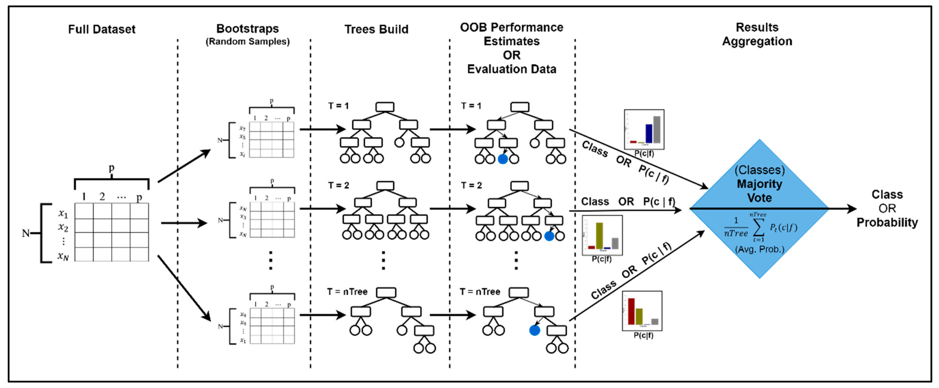
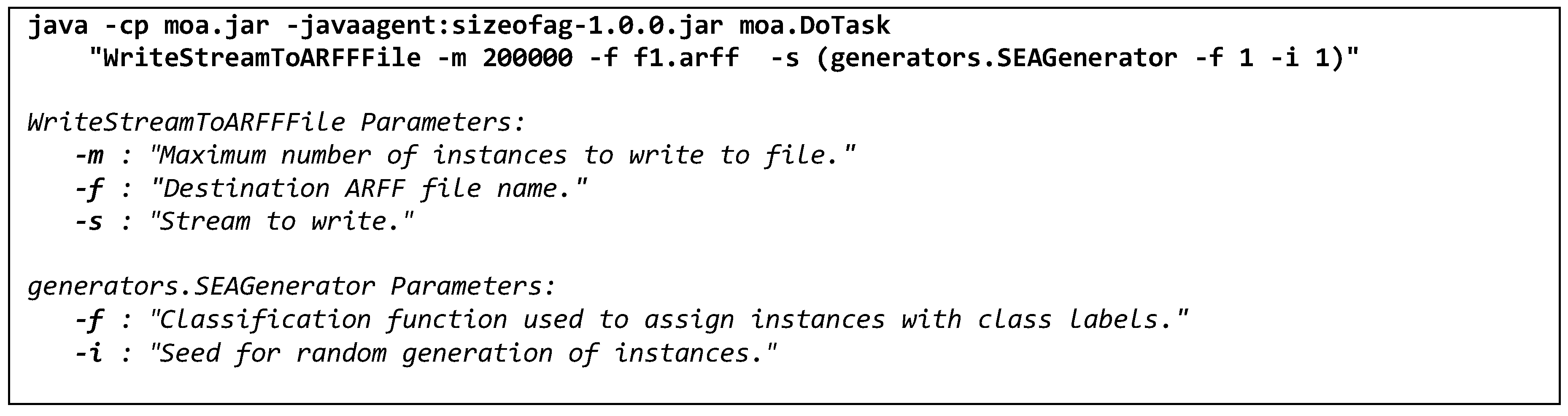
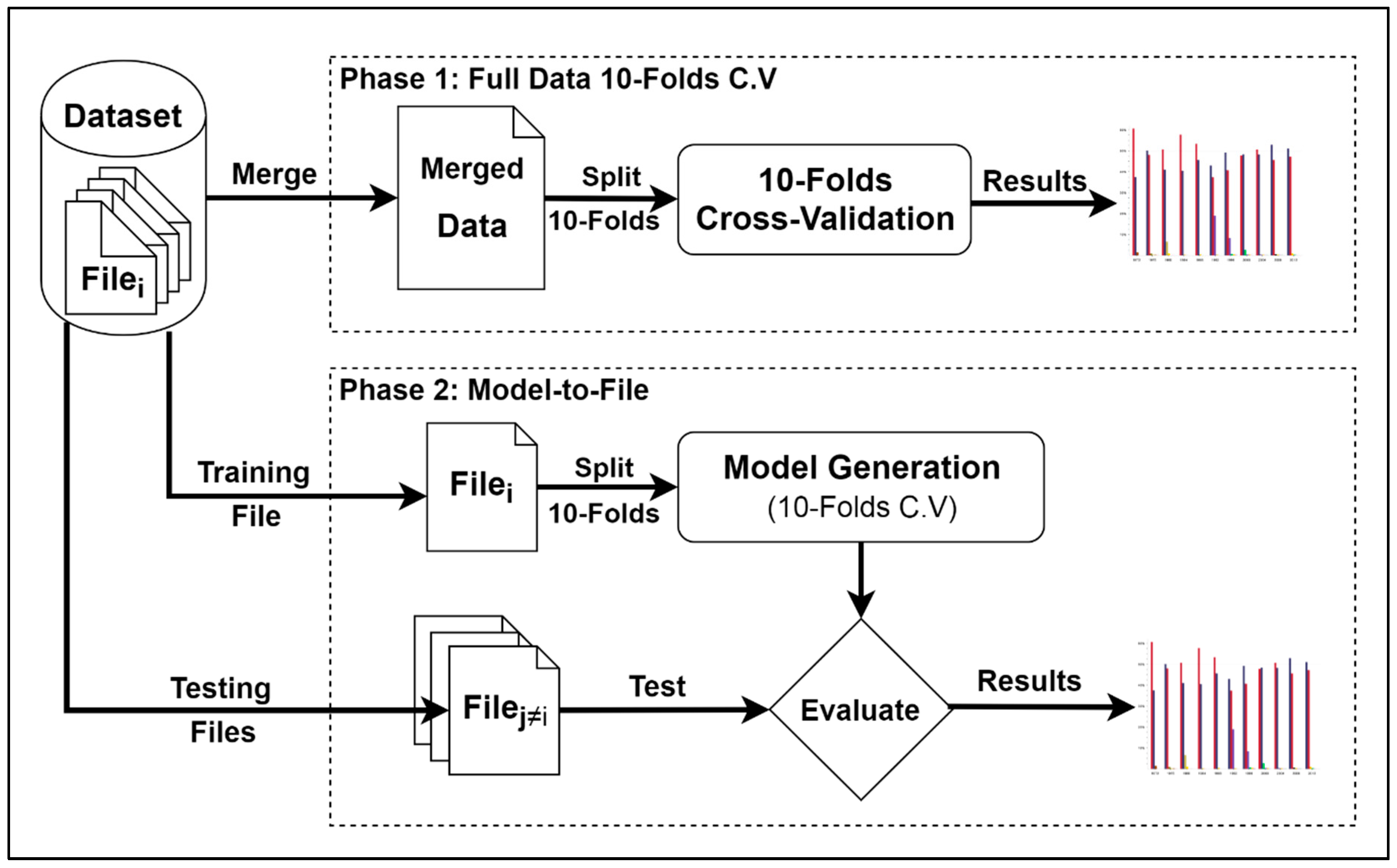
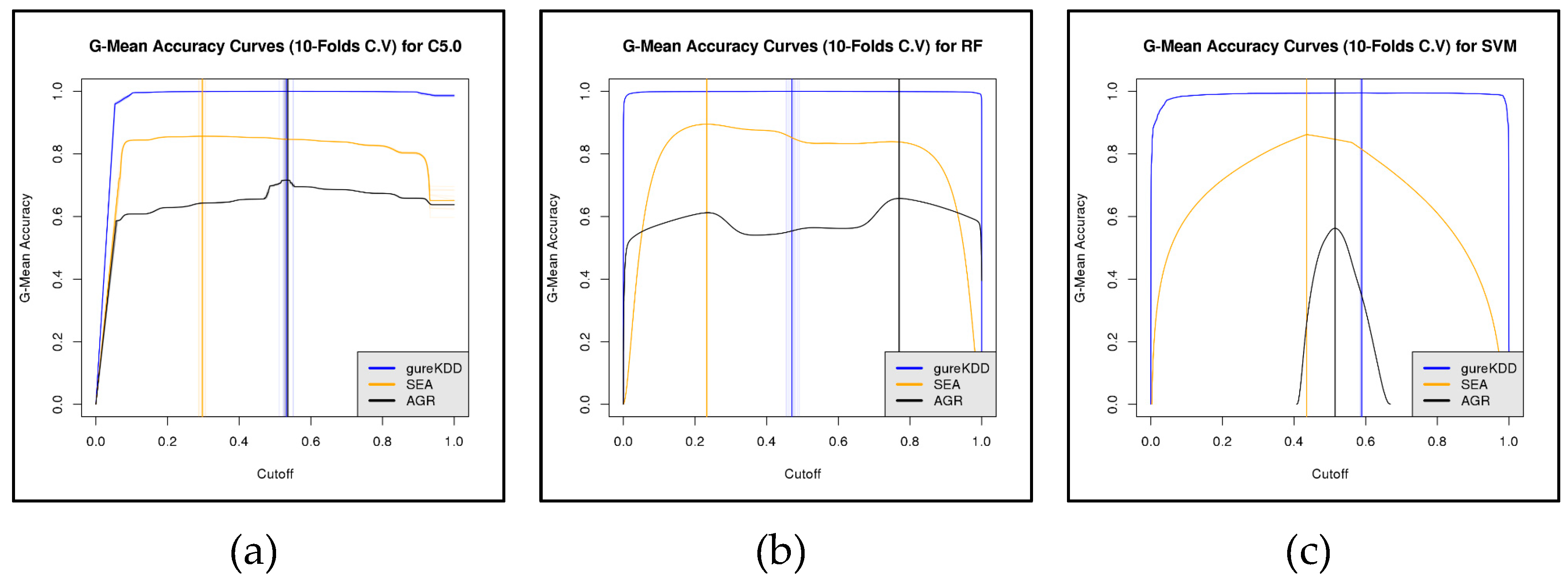
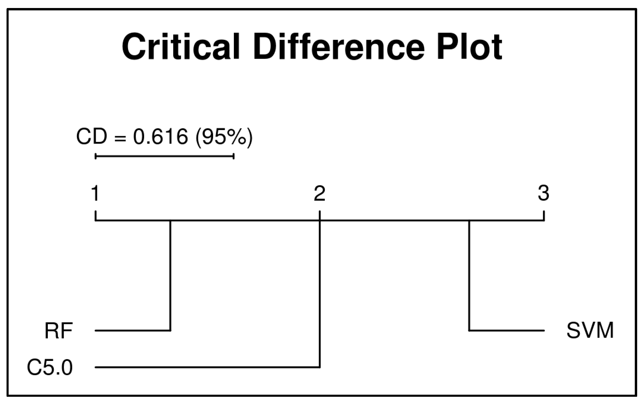
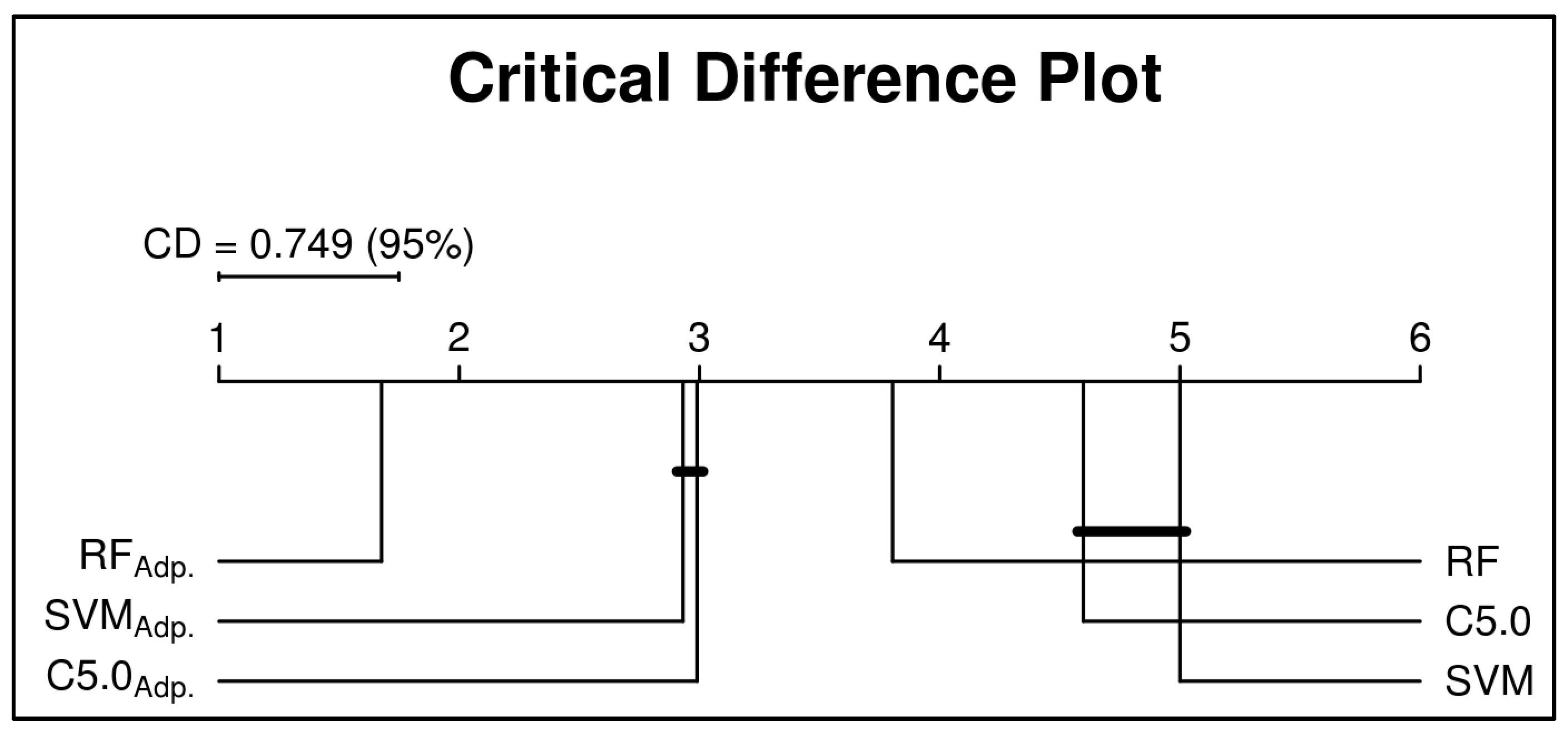
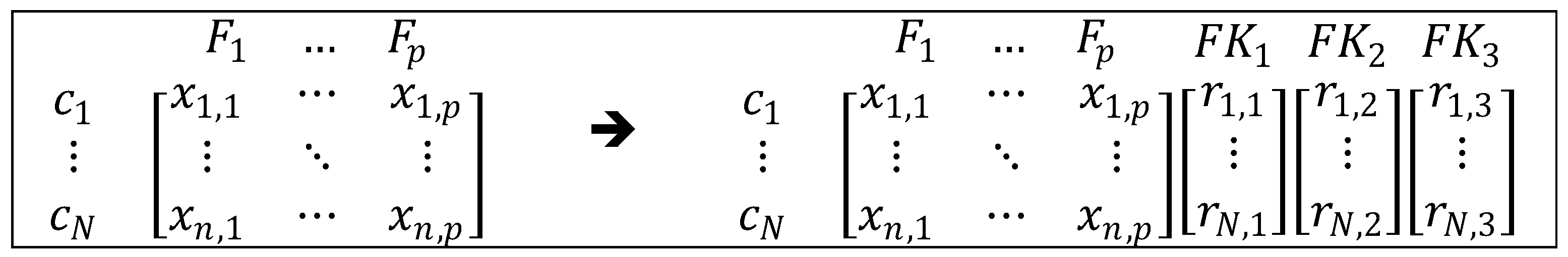
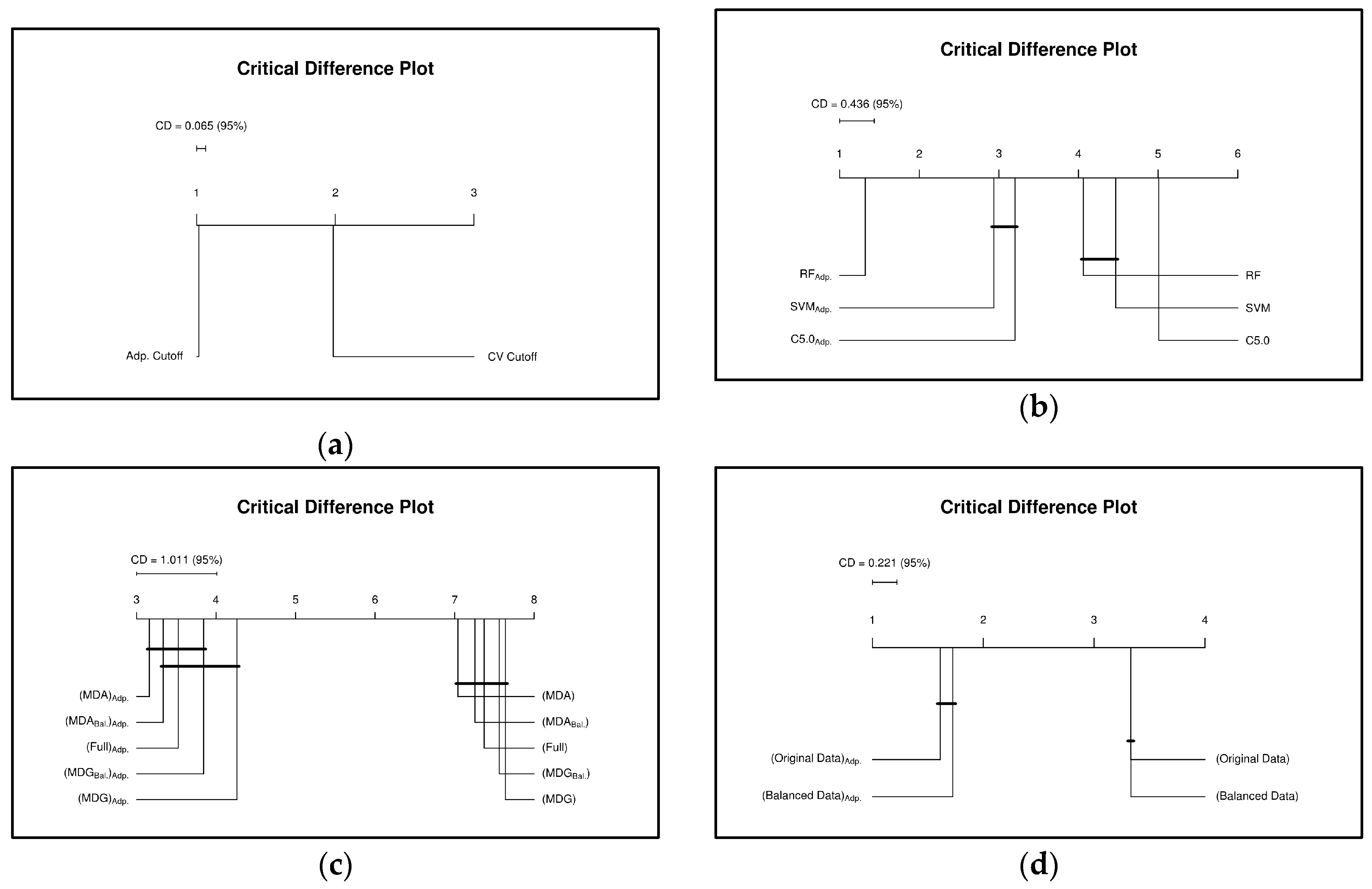
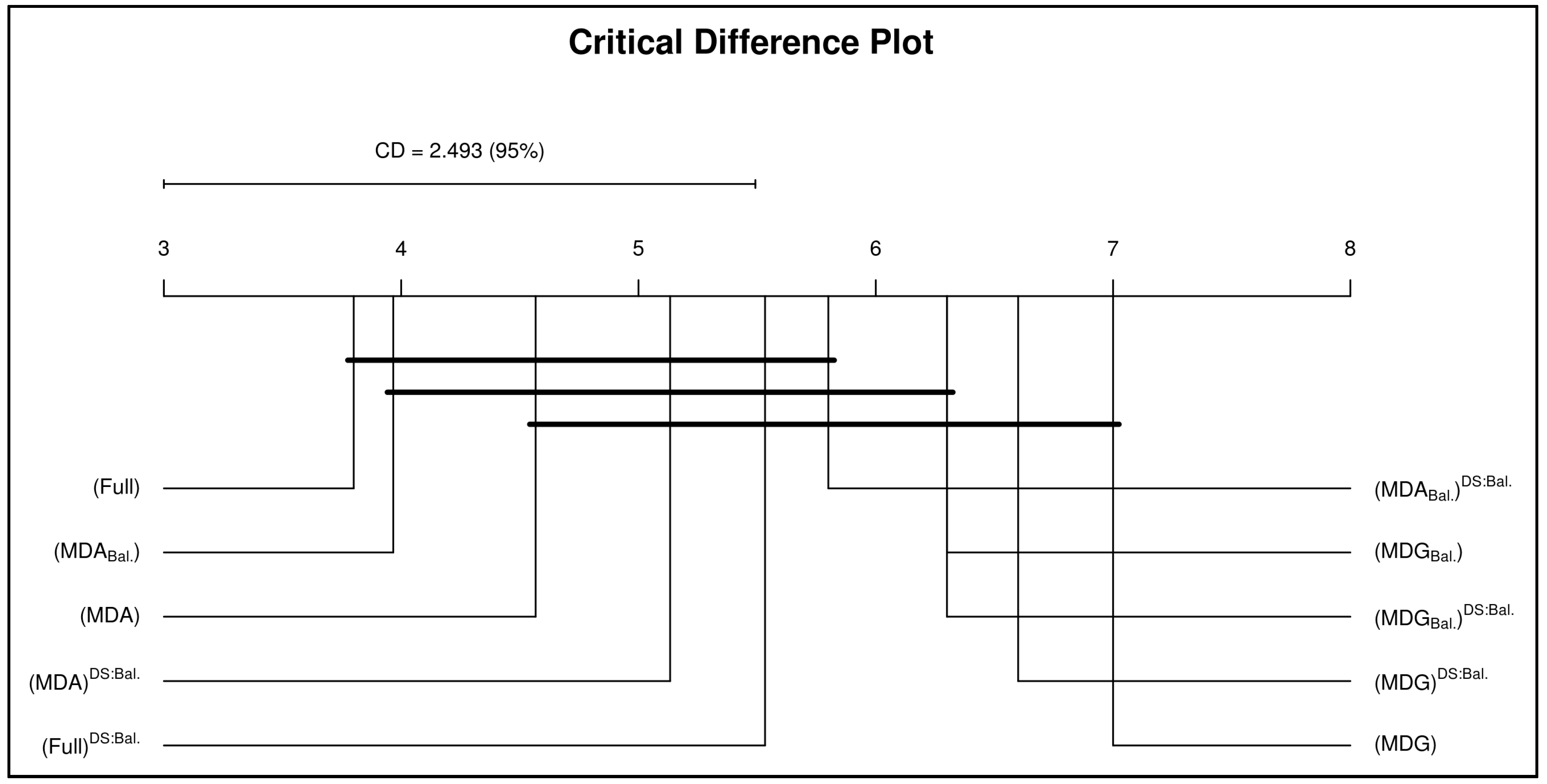
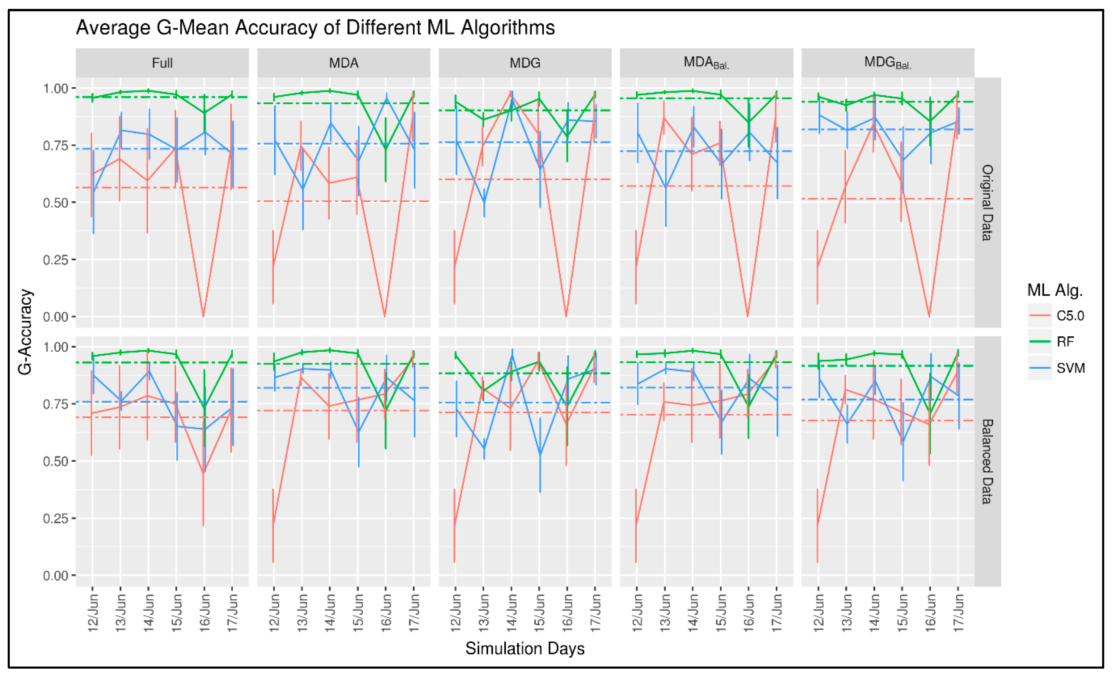
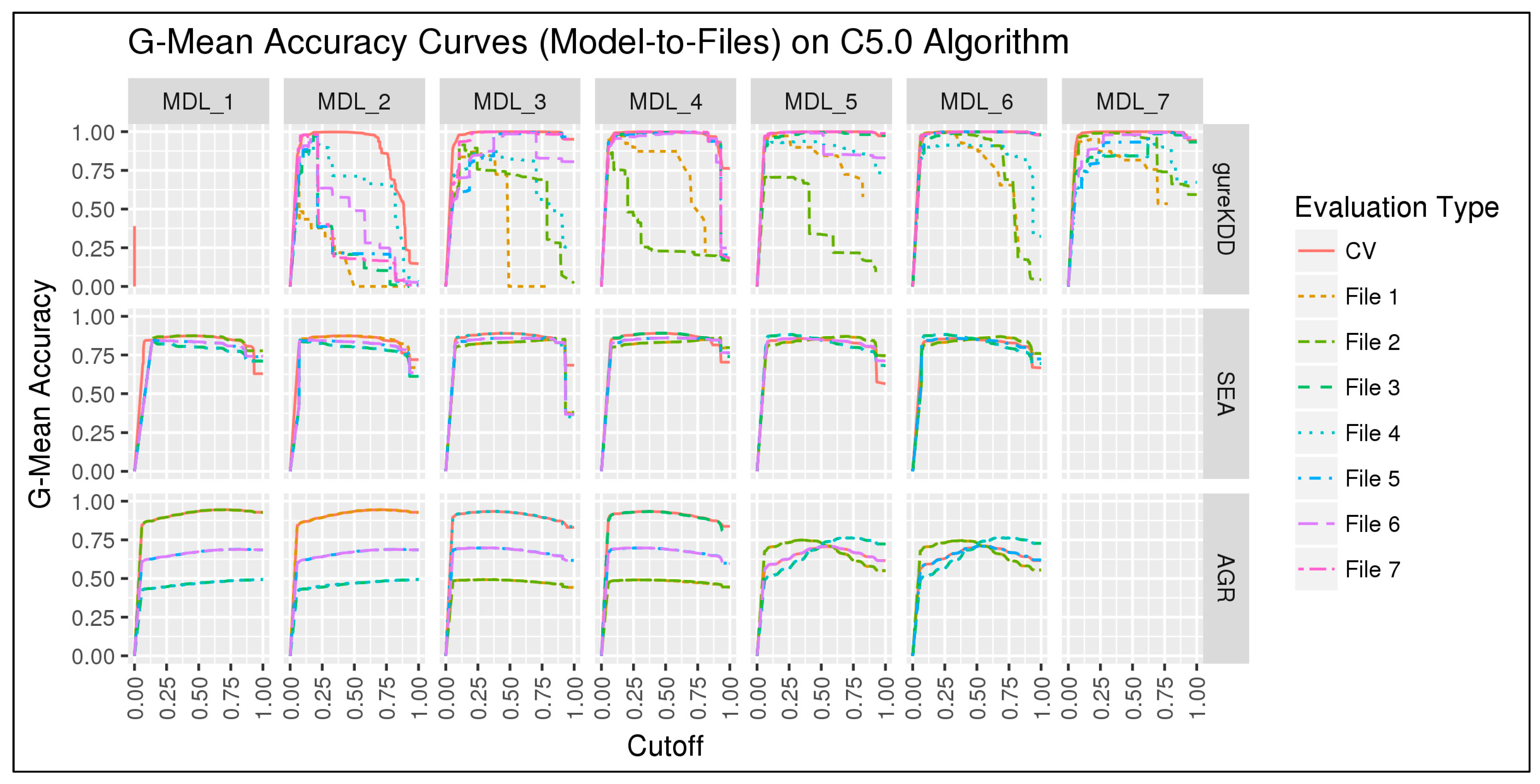
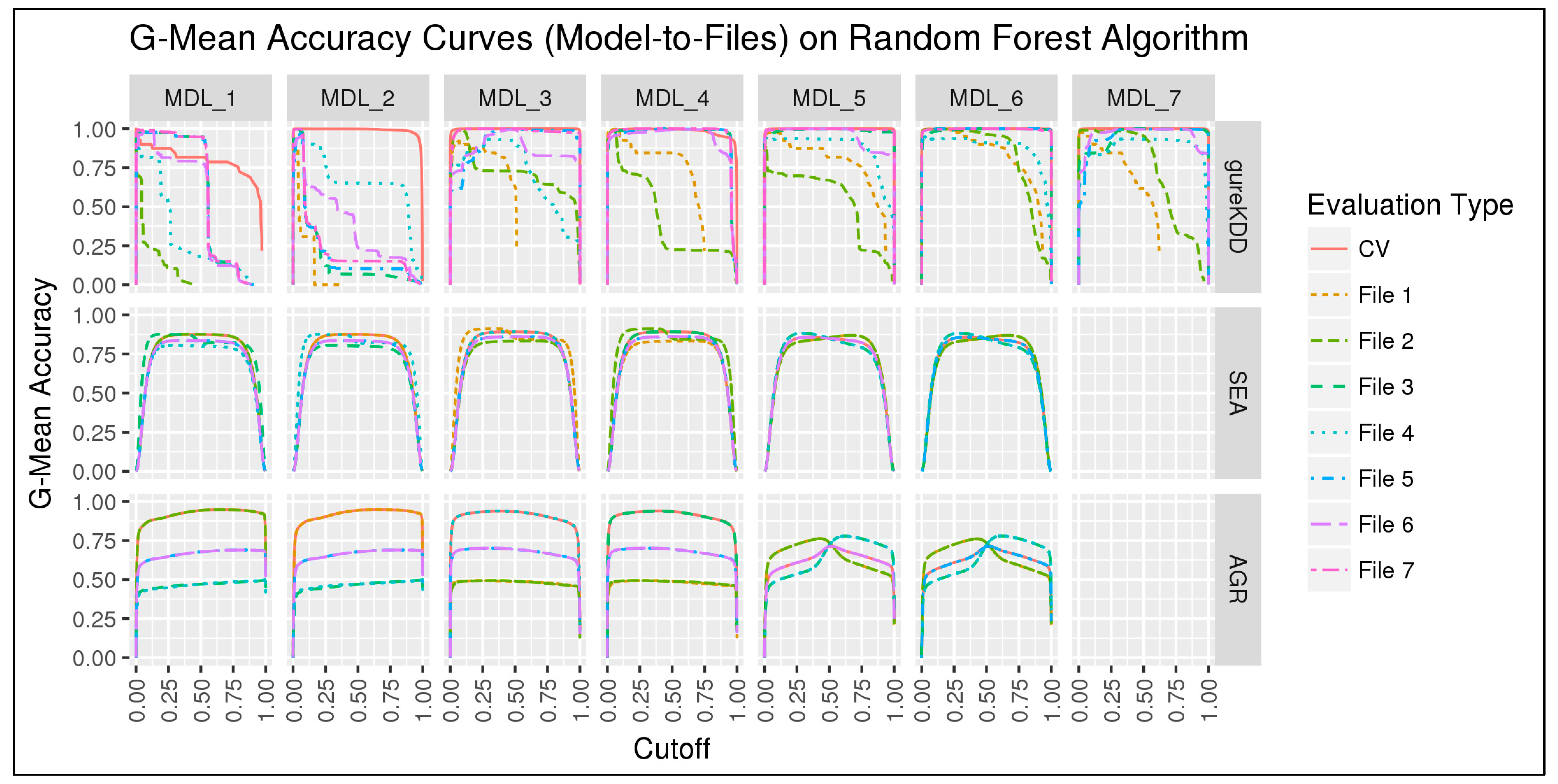
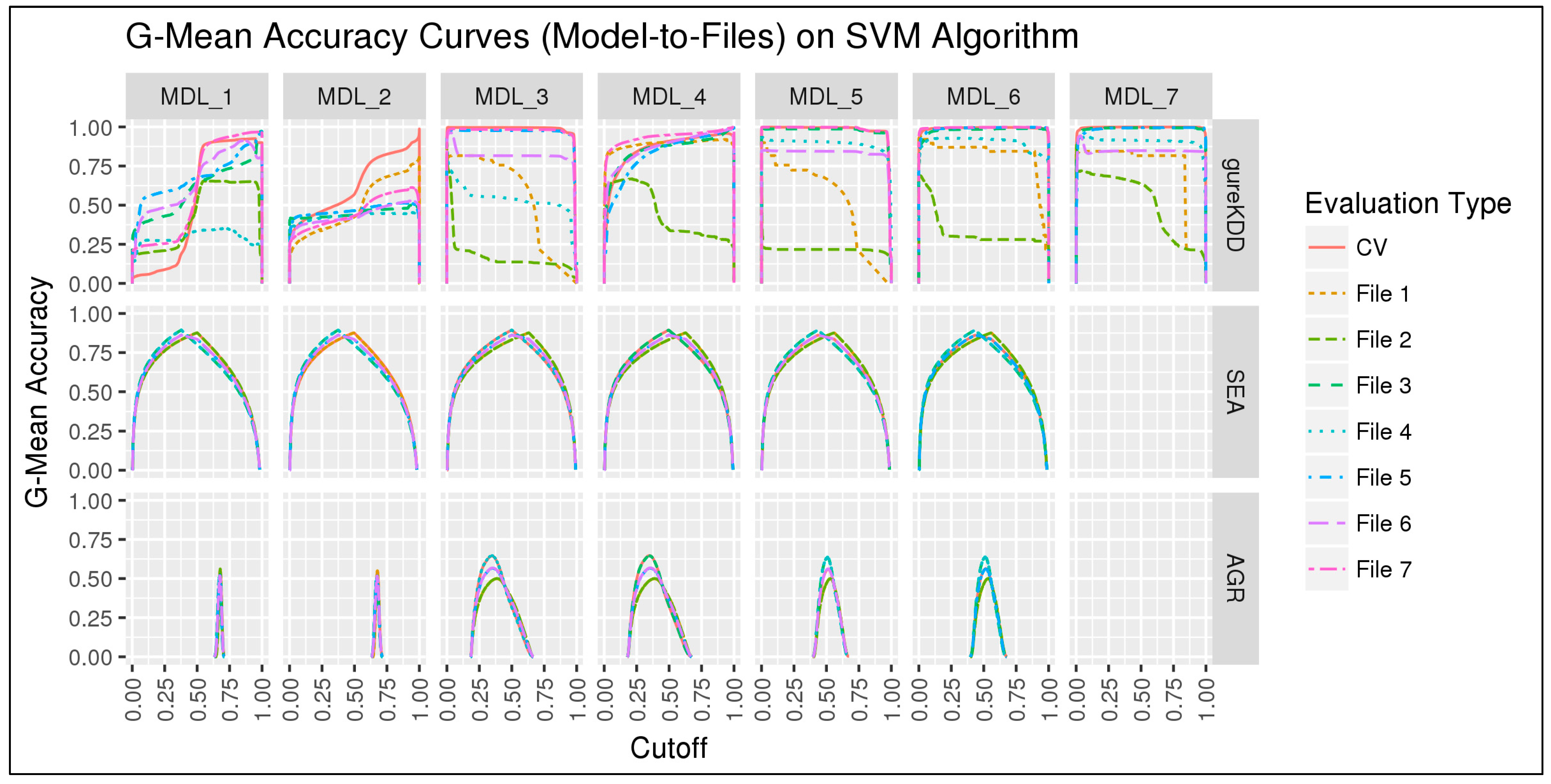
Table A1.
C5.0 model’s performance on different datasets with various effects (before and after threshold adaptation).
Table A1.
C5.0 model’s performance on different datasets with various effects (before and after threshold adaptation).
| File 1 | File 2 | File 3 | File 4 | File 5 | File 6 | File 7 | ||
|---|---|---|---|---|---|---|---|---|
| gureKDD | Model 1 | 0.3904 | 0.0000 0.0000 | 0.0000 0.0000 | 0.0000 0.0000 | 0.0000 0.0000 | 0.0000 0.0000 | 0.0000 0.0000 |
| Model 2 | 0.2181 0.8125 | 0.9981 | 0.2108 0.9740 | 0.7154 0.9248 | 0.2162 0.9715 | 0.5786 0.9646 | 0.1850 0.9805 | |
| Model 3 | 0.0000 0.8884 | 0.7127 0.9150 | 0.9995 | 0.8198 0.8997 | 0.9874 0.9956 | 0.9849 0.9928 | 0.9981 0.9994 | |
| Model 4 | 0.8727 0.9770 | 0.4109 0.8656 | 0.9948 0.9949 | 0.9981 | 0.9862 0.9965 | 0.9740 0.9944 | 0.9988 0.9995 | |
| Model 5 | 0.8448 0.9740 | 0.3315 0.7145 | 0.9963 0.9965 | 0.9107 0.9453 | 0.9998 | 0.8525 0.9977 | 0.9995 0.9995 | |
| Model 6 | 0.8451 0.9997 | 0.9610 0.9948 | 0.9986 0.9989 | 0.9093 0.9128 | 0.9996 0.9997 | 0.9998 | 0.9994 0.9994 | |
| Model 7 | 0.8161 0.9504 | 0.9894 0.9903 | 0.8435 0.9908 | 0.8454 0.9308 | 0.9321 0.9959 | 0.9802 0.9939 | 0.9998 | |
| SEA | Model 1 | 0.8731 | 0.8740 0.8744 | 0.8046 0.8517 | 0.8052 0.8522 | 0.8361 0.8502 | 0.8362 0.8503 | No results as there were only 6 files. |
| Model 2 | 0.8726 0.8736 | 0.8731 | 0.8086 0.8486 | 0.8074 0.8493 | 0.8373 0.8471 | 0.8372 0.8468 | ||
| Model 3 | 0.8320 0.8574 | 0.8319 0.8586 | 0.8898 | 0.8896 0.8901 | 0.8592 0.8599 | 0.8593 0.8600 | ||
| Model 4 | 0.8317 0.8612 | 0.8319 0.8617 | 0.8906 0.8906 | 0.8902 | 0.8599 0.8603 | 0.8599 0.8603 | ||
| Model 5 | 0.8387 0.8700 | 0.8394 0.8704 | 0.8781 0.8821 | 0.8775 0.8821 | 0.2959 0.8567 | 0.8568 0.8569 | ||
| Model 6 | 0.8391 0.8686 | 0.8395 0.8691 | 0.8762 0.8819 | 0.8759 0.8821 | 0.8563 0.8570 | 0.8559 | ||
| AGR | Model 1 | 0.9449 | 0.9443 0.9445 | 0.4844 0.4932 | 0.4850 0.4930 | 0.6873 0.6888 | 0.6873 0.6885 | No results as there were only 6 files. |
| Model 2 | 0.9447 0.9448 | 0.9448 | 0.4835 0.4938 | 0.4829 0.4934 | 0.6871 0.6882 | 0.6867 0.6882 | ||
| Model 3 | 0.4925 0.4932 | 0.4925 0.4929 | 0.9341 | 0.9341 0.9341 | 0.6968 0.6984 | 0.6976 0.6990 | ||
| Model 4 | 0.4907 0.4916 | 0.4900 0.4911 | 0.9328 0.9334 | 0.9339 | 0.6956 0.6977 | 0.6964 0.6985 | ||
| Model 5 | 0.7114 0.7492 | 0.7114 0.7484 | 0.7382 0.7623 | 0.7386 0.7624 | 0.7059 | 0.7079 0.7081 | ||
| Model 6 | 0.7147 0.7463 | 0.7140 0.7459 | 0.7360 0.7626 | 0.7376 0.7628 | 0.7082 0.7085 | 0.7101 | ||
Figure A1.
The gAcc curves for the C5.0 algorithm (see Table A1).
Figure A1.
The gAcc curves for the C5.0 algorithm (see Table A1).

Table A2.
Random Forest (RF) model’s performance on different datasets with various effects (before and after threshold adaptation).
Table A2.
Random Forest (RF) model’s performance on different datasets with various effects (before and after threshold adaptation).
| File 1 | File 2 | File 3 | File 4 | File 5 | File 6 | File 7 | ||
|---|---|---|---|---|---|---|---|---|
| gureKDD | Model 1 | 0.9987 | 0.9752 0.9777 | 0.8538 0.9914 | 0.7948 0.9423 | 0.6733 0.9937 | 0.7410 0.9929 | 0.9673 0.9952 |
| Model 2 | 0.3085 0.9930 | 0.9984 | 0.9807 0.9851 | 0.9103 0.9359 | 0.9657 0.9699 | 0.9531 0.9563 | 0.9859 0.9963 | |
| Model 3 | 0.2182 0.9205 | 0.6430 0.9902 | 0.9996 | 0.5304 0.9324 | 0.9898 0.9951 | 0.8262 0.9930 | 0.9815 0.9994 | |
| Model 4 | 0.8448 0.9970 | 0.7060 0.9894 | 0.9953 0.9966 | 0.9983 | 0.9862 0.9990 | 0.9747 0.9947 | 0.9987 0.9995 | |
| Model 5 | 0.8165 0.9736 | 0.6326 0.8836 | 0.9968 0.9969 | 0.9311 0.9418 | 0.9999 | 0.9980 0.9981 | 0.9996 0.9996 | |
| Model 6 | 0.8863 0.9981 | 0.9542 0.9965 | 0.9989 0.9991 | 0.9082 0.9486 | 0.9998 0.9998 | 0.9999 | 0.9994 0.9996 | |
| Model 7 | 0.8448 0.9754 | 0.9841 0.9908 | 0.9884 0.9986 | 0.9300 0.9352 | 0.9914 0.9970 | 0.9961 0.9974 | 0.9999 | |
| SEA | Model 1 | 0.8750 | 0.8758 0.8758 | 0.8696 0.8764 | 0.8027 0.8053 | 0.8358 0.8364 | 0.8358 0.8364 | No results as there were only 6 files. |
| Model 2 | 0.8752 0.8752 | 0.8757 | 0.8026 0.8053 | 0.8680 0.8759 | 0.8357 0.8363 | 0.8357 0.8363 | ||
| Model 3 | 0.8536 0.9113 | 0.8323 0.8338 | 0.8920 | 0.8924 0.8926 | 0.8609 0.8610 | 0.8604 0.8607 | ||
| Model 4 | 0.8319 0.8333 | 0.8636 0.9113 | 0.8921 0.8921 | 0.8925 | 0.8609 0.8612 | 0.8606 0.8609 | ||
| Model 5 | 0.8389 0.8685 | 0.8393 0.8695 | 0.8782 0.8832 | 0.8786 0.8839 | 0.8576 | 0.8572 0.8576 | ||
| Model 6 | 0.8369 0.8691 | 0.8368 0.8695 | 0.8806 0.8829 | 0.8815 0.8835 | 0.8579 0.8579 | 0.8574 | ||
| AGR | Model 1 | 0.9483 | 0.9482 0.9484 | 0.4774 0.5042 | 0.4812 0.5040 | 0.6869 0.6895 | 0.6871 0.6893 | No results as there were only 6 files. |
| Model 2 | 0.9488 0.9490 | 0.9486 | 0.4788 0.5059 | 0.4762 0.5054 | 0.6858 0.6894 | 0.6856 0.6895 | ||
| Model 3 | 0.4900 0.4939 | 0.4933 0.4940 | 0.9387 | 0.9387 0.9395 | 0.6989 0.7007 | 0.6995 0.7019 | ||
| Model 4 | 0.4928 0.4939 | 0.4902 0.4942 | 0.9390 0.9391 | 0.9398 | 0.6995 0.7011 | 0.6997 0.7016 | ||
| Model 5 | 0.7208 0.7620 | 0.7212 0.7620 | 0.7401 0.7785 | 0.7402 0.7779 | 0.7127 | 0.7144 0.7149 | ||
| Model 6 | 0.7248 0.7607 | 0.7243 0.7608 | 0.7351 0.7788 | 0.7367 0.7805 | 0.7139 0.7140 | 0.7129 | ||
Figure A2.
The gAcc curves for Random Forest algorithm (see Table A2).
Figure A2.
The gAcc curves for Random Forest algorithm (see Table A2).

Table A3.
SVM model’s performance on different datasets with various effects (before and after threshold adaptation).
Table A3.
SVM model’s performance on different datasets with various effects (before and after threshold adaptation).
| File 1 | File 2 | File 3 | File 4 | File 5 | File 6 | File 7 | ||
|---|---|---|---|---|---|---|---|---|
| gureKDD | Model 1 | 0.9250 | 0.6471 0.6545 | 0.8171 0.9727 | 0.2401 0.3504 | 0.8974 0.9695 | 0.8250 0.9123 | 0.9665 0.9715 |
| Model 2 | 0.0000 0.8253 | 0.9869 | 0.1701 0.5024 | 0.3076 0.4525 | 0.1176 0.5163 | 0.3457 0.5285 | 0.1116 0.6131 | |
| Model 3 | 0.8092 0.8303 | 0.7206 0.9022 | 0.9977 | 0.7544 0.9028 | 0.9699 0.9793 | 0.9583 0.9636 | 0.9791 0.9878 | |
| Model 4 | 0.9195 0.9196 | 0.2794 0.6683 | 0.9678 0.9941 | 0.9591 | 0.9766 0.9958 | 0.9783 0.9840 | 0.9867 0.9986 | |
| Model 5 | 0.8724 0.9757 | 0.2233 0.6778 | 0.9865 0.9922 | 0.9172 0.9339 | 0.9992 | 0.8503 0.8507 | 0.9983 0.9985 | |
| Model 6 | 0.8443 0.9531 | 0.2804 0.6929 | 0.9894 0.9907 | 0.9145 0.9270 | 0.9976 0.9979 | 0.9970 | 0.9986 0.9986 | |
| Model 7 | 0.8165 0.8518 | 0.3163 0.8853 | 0.9944 0.9944 | 0.9107 0.9366 | 0.9960 0.9962 | 0.8476 0.9434 | 0.9994 | |
| SEA | Model 1 | 0.8763 | 0.8771 0.8771 | 0.8018 0.8936 | 0.8016 0.8941 | 0.8358 0.8617 | 0.8360 0.8615 | No results as there were only 6 files. |
| Model 2 | 0.8759 0.8760 | 0.8765 | 0.8021 0.8928 | 0.8018 0.8933 | 0.8356 0.8613 | 0.8359 0.8610 | ||
| Model 3 | 0.8319 0.8763 | 0.8320 0.8770 | 0.8933 | 0.8939 0.8940 | 0.8615 0.8617 | 0.8613 0.8615 | ||
| Model 4 | 0.8319 0.8763 | 0.8321 0.8769 | 0.8933 0.8933 | 0.8938 | 0.8615 0.8616 | 0.8612 0.8613 | ||
| Model 5 | 0.8325 0.8759 | 0.8326 0.8765 | 0.8924 0.8928 | 0.8929 0.8932 | 0.8614 | 0.8610 0.8611 | ||
| Model 6 | 0.8331 0.8756 | 0.8332 0.8760 | 0.8914 0.8923 | 0.8918 0.8927 | 0.8612 0.8612 | 0.8609 | ||
| AGR | Model 1 | 0.5529 | 0.5614 0.5615 | 0.4695 0.5106 | 0.4676 0.5079 | 0.5148 0.5211 | 0.5112 0.5178 | No results as there were only 6 files. |
| Model 2 | 0.5494 0.5498 | 0.5479 | 0.4829 0.5045 | 0.4813 0.5032 | 0.5148 0.5174 | 0.5125 0.5161 | ||
| Model 3 | 0.4879 0.4995 | 0.4877 0.5004 | 0.6440 | 0.6460 0.6462 | 0.5656 0.5659 | 0.5676 0.5685 | ||
| Model 4 | 0.4862 0.4991 | 0.4861 0.5005 | 0.6450 0.6453 | 0.6467 | 0.5652 0.5664 | 0.5673 0.5688 | ||
| Model 5 | 0.4867 0.4990 | 0.4862 0.5003 | 0.6338 0.6348 | 0.6352 0.6365 | 0.5598 | 0.5620 0.5623 | ||
| Model 6 | 0.4892 0.4996 | 0.4889 0.5006 | 0.6357 0.6374 | 0.6362 0.6384 | 0.5615 0.5617 | 0.5632 | ||
Figure A3.
The gAcc curves for the SVM algorithm (see Table A3).
Figure A3.
The gAcc curves for the SVM algorithm (see Table A3).

Table A4.
The gAcc of models for the fixed optimal (CV) and adapted cut-off (threshold) for the C5.0 algorithm.
Table A4.
The gAcc of models for the fixed optimal (CV) and adapted cut-off (threshold) for the C5.0 algorithm.
| Original | Balance | ||||||||||||
|---|---|---|---|---|---|---|---|---|---|---|---|---|---|
| Day 2 | Day 3 | Day 4 | Day 5 | Day 6 | Day 7 | Day 2 | Day 3 | Day 4 | Day 5 | Day 6 | Day 7 | ||
| Full | MDL 2 | 0.9996 | 0.0099 | 0.0176 | 0.0053 | 0.8062 | 0.0568 | 0.9999 | 0.0100 | 0.0241 | 0.0053 | 0.8995 | 0.0562 |
| 0.5882 | 0.5045 | 0.0148 | 0.9999 | 0.9934 | 0.9044 | 0.6387 | 0.0144 | 1.0000 | 0.9879 | ||||
| MDL 3 | 0.5967 | 0.9834 | 0.8106 | 0.0105 | 0.0000 | 0.9477 | 0.9014 | 0.9823 | 0.8661 | 0.0130 | 0.6304 | 0.7753 | |
| 0.9745 | 0.9137 | 0.0211 | 0.5650 | 0.9776 | 0.9487 | 0.9043 | 0.0134 | 0.9652 | 0.8440 | ||||
| MDL 4 | 0.0375 | 0.9373 | 0.9813 | 0.0000 | 0.0000 | 0.0316 | 0.9916 | 0.9249 | 0.9815 | 0.0129 | 0.9985 | 0.7109 | |
| 0.9937 | 0.9507 | 0.0130 | 0.9514 | 0.0616 | 0.9931 | 0.9271 | 0.0176 | 0.9989 | 0.9900 | ||||
| MDL 5 | 0.9982 | 0.0000 | 0.0216 | 0.9977 | 0.9045 | 0.0875 | 0.8820 | 0.0100 | 0.3610 | 0.9975 | 0.8523 | 0.7759 | |
| 0.9993 | 0.1950 | 0.4956 | 0.9999 | 0.9895 | 0.9934 | 0.1419 | 0.6242 | 0.9966 | 0.9907 | ||||
| MDL 6 | 0.0000 | 0.0000 | 0.0000 | 0.0000 | 0.4606 | 0.0000 | 0.9910 | 0.0200 | 0.0250 | 0.0479 | 1.0000 | 0.7458 | |
| 0.0000 | 0.0000 | 0.0000 | 0.0000 | 0.0000 | 0.9988 | 0.1485 | 0.0278 | 0.0480 | 0.9980 | ||||
| MDL 7 | 0.9901 | 0.9151 | 0.4357 | 0.0043 | 0.9998 | 0.9999 | 0.9956 | 0.3826 | 0.3916 | 0.0092 | 0.9999 | 1.0000 | |
| 0.9945 | 0.9413 | 0.7629 | 0.0132 | 0.9998 | 0.9962 | 0.9210 | 0.6703 | 0.0258 | 1.0000 | ||||
| MDA | MDL 2 | 0.9998 | 0.0000 | 0.0279 | 0.0479 | 0.8528 | 0.0568 | 1.0000 | 0.0000 | 0.0279 | 0.0479 | 0.8528 | 0.0568 |
| 0.0940 | 0.0279 | 0.0479 | 0.8528 | 0.0568 | 0.0940 | 0.0279 | 0.0479 | 0.8528 | 0.0568 | ||||
| MDL 3 | 0.9814 | 0.9838 | 0.5062 | 0.2146 | 0.7327 | 0.1403 | 0.5278 | 0.9826 | 0.8504 | 0.8807 | 0.8344 | 0.8673 | |
| 0.9845 | 0.5720 | 0.7332 | 0.9890 | 0.4531 | 0.7520 | 0.8558 | 0.9420 | 0.8395 | 0.9405 | ||||
| MDL 4 | 0.1127 | 0.8999 | 0.9802 | 0.0402 | 0.3013 | 0.0283 | 0.7905 | 0.9193 | 0.9800 | 0.0790 | 0.9985 | 0.0647 | |
| 0.6653 | 0.9476 | 0.3447 | 0.8502 | 0.1108 | 0.9882 | 0.9299 | 0.3659 | 0.9992 | 0.4175 | ||||
| MDL 5 | 0.9902 | 0.0100 | 0.0983 | 0.9977 | 0.8528 | 0.0550 | 0.9087 | 0.0100 | 0.6697 | 0.9974 | 0.9478 | 0.8538 | |
| 0.9990 | 0.4568 | 0.4944 | 0.9504 | 0.1438 | 0.9857 | 0.0378 | 0.8277 | 0.9896 | 0.9923 | ||||
| MDL 6 | 0.0000 | 0.0000 | 0.0000 | 0.0000 | 0.4606 | 0.0000 | 0.9808 | 0.0141 | 0.0128 | 0.0473 | 1.0000 | 0.0532 | |
| 0.0000 | 0.0000 | 0.0000 | 0.0000 | 0.0000 | 1.0000 | 0.8035 | 0.4143 | 0.7486 | 0.9999 | ||||
| MDL 7 | 0.9923 | 0.8980 | 0.4348 | 0.0485 | 0.9998 | 0.9998 | 0.9469 | 0.1264 | 0.0249 | 0.7837 | 1.0000 | 0.9998 | |
| 0.9976 | 0.9286 | 0.4498 | 0.9837 | 1.0000 | 0.9940 | 0.9236 | 0.8137 | 0.9907 | 1.0000 | ||||
| MDG | MDL 2 | 0.9998 | 0.0000 | 0.0279 | 0.0479 | 0.8528 | 0.0568 | 1.0000 | 0.0000 | 0.0279 | 0.0479 | 0.8528 | 0.0568 |
| 0.0940 | 0.0279 | 0.0479 | 0.8528 | 0.0568 | 0.0940 | 0.0279 | 0.0479 | 0.8528 | 0.0568 | ||||
| MDL 3 | 0.1309 | 0.9702 | 0.8138 | 0.5949 | 0.0000 | 0.6922 | 0.4031 | 0.9656 | 0.8976 | 0.5522 | 0.5120 | 0.7539 | |
| 0.8279 | 0.8979 | 0.7917 | 0.4171 | 0.7796 | 0.8978 | 0.9092 | 0.6895 | 0.7127 | 0.8859 | ||||
| MDL 4 | 0.6496 | 0.9160 | 0.9431 | 0.9906 | 0.0000 | 0.9976 | 0.5688 | 0.8835 | 0.9165 | 0.9049 | 0.0000 | 0.9666 | |
| 0.9799 | 0.9246 | 0.9912 | 0.9815 | 0.9977 | 0.8639 | 0.9026 | 0.9100 | 0.0000 | 0.9792 | ||||
| MDL 5 | 0.9208 | 0.0200 | 0.0176 | 0.9969 | 0.0000 | 0.9611 | 0.9927 | 0.0141 | 0.3249 | 0.9972 | 0.8519 | 0.9978 | |
| 0.9896 | 0.2523 | 0.8186 | 0.9529 | 0.9836 | 0.9961 | 0.8160 | 0.8821 | 0.9965 | 0.9982 | ||||
| MDL 6 | 0.0000 | 0.0000 | 0.0000 | 0.0000 | 0.4606 | 0.0000 | 0.0614 | 0.0100 | 0.0000 | 0.0092 | 1.0000 | 0.0142 | |
| 0.0000 | 0.0000 | 0.0000 | 0.0000 | 0.0000 | 0.9935 | 0.8094 | 0.4154 | 0.0822 | 0.9993 | ||||
| MDL 7 | 0.9943 | 0.8910 | 0.4342 | 0.0485 | 0.9999 | 0.9999 | 0.9867 | 0.9068 | 0.4390 | 0.5440 | 0.9525 | 0.9997 | |
| 0.9976 | 0.9253 | 0.4423 | 0.9837 | 1.0000 | 0.9944 | 0.9142 | 0.6559 | 0.9853 | 0.9962 | ||||
| MDABal. | MDL 2 | 0.9998 | 0.0000 | 0.0279 | 0.0479 | 0.8528 | 0.0568 | 1.0000 | 0.0000 | 0.0279 | 0.0479 | 0.8528 | 0.0568 |
| 0.0940 | 0.0279 | 0.0479 | 0.8528 | 0.0568 | 0.0940 | 0.0279 | 0.0479 | 0.8528 | 0.0568 | ||||
| MDL 3 | 0.9849 | 0.9833 | 0.5069 | 0.8782 | 0.5156 | 0.4736 | 0.7077 | 0.9821 | 0.6074 | 0.5015 | 0.7124 | 0.0816 | |
| 0.9876 | 0.5967 | 0.9296 | 0.9843 | 0.8484 | 0.8853 | 0.8378 | 0.8607 | 0.7731 | 0.4364 | ||||
| MDL 4 | 0.1337 | 0.9435 | 0.9802 | 0.0580 | 0.3013 | 0.0245 | 0.9852 | 0.6290 | 0.9805 | 0.0627 | 0.9958 | 0.4256 | |
| 0.6646 | 0.9492 | 0.9824 | 0.8496 | 0.1062 | 0.9906 | 0.9232 | 0.1455 | 0.9971 | 0.6606 | ||||
| MDL 5 | 0.9984 | 0.1142 | 0.0993 | 0.9977 | 0.7977 | 0.0568 | 0.8156 | 0.0100 | 0.0278 | 0.9974 | 0.7368 | 0.3558 | |
| 0.9995 | 0.4586 | 0.7236 | 0.9367 | 0.6729 | 0.9888 | 0.1569 | 0.6789 | 0.9954 | 0.9915 | ||||
| MDL 6 | 0.0000 | 0.0000 | 0.0000 | 0.0000 | 0.4606 | 0.0000 | 0.0614 | 0.0100 | 0.0125 | 0.0092 | 1.0000 | 0.0142 | |
| 0.0000 | 0.0000 | 0.0000 | 0.0000 | 0.0000 | 0.9985 | 0.8062 | 0.4115 | 0.7465 | 0.9996 | ||||
| MDL 7 | 0.9923 | 0.8952 | 0.4348 | 0.0485 | 0.9998 | 0.9998 | 0.9873 | 0.1978 | 0.0892 | 0.7895 | 0.9999 | 0.9998 | |
| 0.9976 | 0.9285 | 0.4445 | 0.9829 | 1.0000 | 0.9940 | 0.9236 | 0.8137 | 0.9907 | 1.0000 | ||||
| MDGBal. | MDL 2 | 0.9998 | 0.0000 | 0.0279 | 0.0479 | 0.8528 | 0.0568 | 1.0000 | 0.0000 | 0.0279 | 0.0479 | 0.8528 | 0.0568 |
| 0.0940 | 0.0279 | 0.0479 | 0.8528 | 0.0568 | 0.0940 | 0.0279 | 0.0479 | 0.8528 | 0.0568 | ||||
| MDL 3 | 0.2910 | 0.9827 | 0.6145 | 0.1415 | 0.0000 | 0.4229 | 0.8819 | 0.9820 | 0.8189 | 0.9222 | 0.5312 | 0.6688 | |
| 0.4477 | 0.8308 | 0.7589 | 0.0000 | 0.8031 | 0.8896 | 0.8388 | 0.9300 | 0.5783 | 0.8254 | ||||
| MDL 4 | 0.6499 | 0.9485 | 0.9811 | 0.9764 | 0.3011 | 0.0567 | 0.9824 | 0.9265 | 0.9803 | 0.7625 | 0.8510 | 0.0615 | |
| 0.9342 | 0.9497 | 0.9799 | 0.9918 | 0.3565 | 0.9826 | 0.9265 | 0.9326 | 0.9341 | 0.0756 | ||||
| MDL 5 | 0.9673 | 0.0158 | 0.1048 | 0.9976 | 0.7977 | 0.0531 | 0.8201 | 0.0000 | 0.0736 | 0.9973 | 0.8510 | 0.4139 | |
| 0.9985 | 0.4339 | 0.4977 | 0.9522 | 0.0680 | 0.9485 | 0.1562 | 0.7646 | 0.9005 | 0.8068 | ||||
| MDL 6 | 0.0000 | 0.0000 | 0.0000 | 0.0000 | 0.4606 | 0.0000 | 0.0614 | 0.0100 | 0.0000 | 0.0092 | 1.0000 | 0.0142 | |
| 0.0000 | 0.0000 | 0.0000 | 0.0000 | 0.0000 | 0.9935 | 0.8094 | 0.4154 | 0.0822 | 0.9993 | ||||
| MDL 7 | 0.9929 | 0.1801 | 0.0729 | 0.7814 | 0.9997 | 0.9998 | 0.9883 | 0.0064 | 0.0139 | 0.0533 | 0.9998 | 0.9999 | |
| 0.9954 | 0.9267 | 0.4813 | 0.9778 | 1.0000 | 0.9900 | 0.9054 | 0.5412 | 0.9913 | 1.0000 | ||||
Table A5.
The gAcc of models for the fixed optimal (CV) and adapted cut-off (threshold) for the Random Forest (RF) algorithm.
Table A5.
The gAcc of models for the fixed optimal (CV) and adapted cut-off (threshold) for the Random Forest (RF) algorithm.
| Original | Balance | ||||||||||||
|---|---|---|---|---|---|---|---|---|---|---|---|---|---|
| Day 2 | Day 3 | Day 4 | Day 5 | Day 6 | Day 7 | Day 2 | Day 3 | Day 4 | Day 5 | Day 6 | Day 7 | ||
| Full | MDL 2 | 1.0000 | 0.0042 | 0.0279 | 0.0482 | 1.0000 | 0.0602 | 1.0000 | 0.0100 | 0.0216 | 0.0476 | 0.9535 | 0.0559 |
| 0.9272 | 0.9478 | 0.9094 | 1.0000 | 0.9987 | 0.9293 | 0.9413 | 0.9257 | 1.0000 | 0.9987 | ||||
| MDL 3 | 0.9521 | 0.9849 | 0.9213 | 0.6884 | 0.8560 | 0.9411 | 0.9663 | 0.9848 | 0.9191 | 0.7498 | 0.9530 | 0.9758 | |
| 0.9932 | 0.9739 | 0.9577 | 0.9870 | 0.9976 | 0.9925 | 0.9688 | 0.9340 | 0.9793 | 0.9987 | ||||
| MDL 4 | 0.9428 | 0.9301 | 0.9827 | 0.8425 | 0.8832 | 0.9404 | 0.9762 | 0.9237 | 0.9829 | 0.8991 | 0.9268 | 0.9688 | |
| 0.9945 | 0.9560 | 0.9920 | 0.9998 | 0.9978 | 0.9948 | 0.9471 | 0.9858 | 0.9997 | 0.9882 | ||||
| MDL 5 | 0.9997 | 0.0133 | 0.0648 | 0.9978 | 0.9535 | 0.0585 | 0.9888 | 0.2259 | 0.6808 | 0.9981 | 0.9934 | 0.9925 | |
| 0.9999 | 0.9205 | 0.9395 | 1.0000 | 0.9976 | 0.9971 | 0.9156 | 0.9302 | 0.9998 | 0.9926 | ||||
| MDL 6 | 0.9912 | 0.0000 | 0.0250 | 0.0479 | 1.0000 | 0.0568 | 0.0217 | 0.0100 | 0.0125 | 0.0053 | 1.0000 | 0.0142 | |
| 1.0000 | 0.9120 | 0.5737 | 0.9671 | 0.9998 | 0.9999 | 0.8685 | 0.6837 | 0.1048 | 0.9998 | ||||
| MDL 7 | 0.9964 | 0.9140 | 0.4314 | 0.7864 | 1.0000 | 1.0000 | 0.0217 | 0.0100 | 0.0125 | 0.0341 | 0.5279 | 1.0000 | |
| 0.9979 | 0.9351 | 0.9340 | 0.9911 | 1.0000 | 0.9998 | 0.9381 | 0.9319 | 0.9755 | 1.0000 | ||||
| MDA | MDL 2 | 1.0000 | 0.0463 | 0.0279 | 0.0482 | 1.0000 | 0.0585 | 1.0000 | 0.0100 | 0.0216 | 0.0476 | 0.8528 | 0.0564 |
| 0.9308 | 0.9417 | 0.9322 | 1.0000 | 0.9983 | 0.9281 | 0.9504 | 0.7999 | 1.0000 | 0.9984 | ||||
| MDL 3 | 0.9790 | 0.9848 | 0.9636 | 0.9089 | 0.9570 | 0.9890 | 0.9683 | 0.9848 | 0.9197 | 0.8158 | 0.8781 | 0.9282 | |
| 0.9895 | 0.9738 | 0.9490 | 0.9844 | 0.9963 | 0.9927 | 0.9690 | 0.9336 | 0.9839 | 0.9983 | ||||
| MDL 4 | 0.9493 | 0.9374 | 0.9826 | 0.8913 | 0.8956 | 0.9448 | 0.9463 | 0.9269 | 0.9827 | 0.8882 | 0.9024 | 0.9467 | |
| 0.9947 | 0.9557 | 0.9917 | 0.9971 | 0.9984 | 0.9948 | 0.9449 | 0.9889 | 0.9993 | 0.9942 | ||||
| MDL 5 | 0.9997 | 0.0141 | 0.0872 | 0.9978 | 0.9535 | 0.0619 | 0.9891 | 0.2439 | 0.6620 | 0.9981 | 0.9935 | 0.9933 | |
| 0.9999 | 0.9162 | 0.9388 | 1.0000 | 0.9951 | 0.9996 | 0.9218 | 0.9411 | 0.9981 | 0.9935 | ||||
| MDL 6 | 0.9983 | 0.0100 | 0.0250 | 0.0479 | 1.0000 | 0.0568 | 0.0217 | 0.0100 | 0.0176 | 0.0053 | 1.0000 | 0.0142 | |
| 1.0000 | 0.8553 | 0.4649 | 0.3326 | 0.9999 | 1.0000 | 0.9320 | 0.4956 | 0.1731 | 1.0000 | ||||
| MDL 7 | 0.9933 | 0.9309 | 0.4459 | 0.9875 | 1.0000 | 1.0000 | 0.0217 | 0.0100 | 0.0125 | 0.0367 | 0.4053 | 1.0000 | |
| 0.9971 | 0.9360 | 0.9370 | 0.9911 | 1.0000 | 0.9998 | 0.9355 | 0.9280 | 0.9699 | 1.0000 | ||||
| MDG | MDL 2 | 1.0000 | 0.0452 | 0.0279 | 0.0482 | 1.0000 | 0.0585 | 1.0000 | 0.0100 | 0.0216 | 0.0473 | 0.8528 | 0.0561 |
| 0.9296 | 0.9317 | 0.8425 | 1.0000 | 0.9982 | 0.9287 | 0.9457 | 0.9430 | 1.0000 | 0.9984 | ||||
| MDL 3 | 0.5035 | 0.9780 | 0.9171 | 0.6307 | 0.0000 | 0.7868 | 0.5308 | 0.9698 | 0.9051 | 0.5622 | 0.0000 | 0.6543 | |
| 0.8340 | 0.9185 | 0.8195 | 0.7887 | 0.9471 | 0.8000 | 0.9112 | 0.7204 | 0.7087 | 0.8924 | ||||
| MDL 4 | 0.7032 | 0.9160 | 0.9432 | 0.9856 | 0.0000 | 0.9884 | 0.6800 | 0.8996 | 0.8906 | 0.9829 | 0.0000 | 0.9531 | |
| 0.7703 | 0.9242 | 0.9913 | 0.8236 | 0.9974 | 0.8676 | 0.9000 | 0.9829 | 0.7499 | 0.9538 | ||||
| MDL 5 | 0.1390 | 0.0100 | 0.0254 | 0.9978 | 0.6742 | 0.0375 | 0.9897 | 0.0223 | 0.5450 | 0.9981 | 0.9999 | 0.3540 | |
| 0.9992 | 0.8518 | 0.9138 | 0.9996 | 0.9976 | 0.9926 | 0.8016 | 0.8817 | 1.0000 | 0.9982 | ||||
| MDL 6 | 0.9982 | 0.0000 | 0.0250 | 0.0479 | 1.0000 | 0.0568 | 0.0217 | 0.0100 | 0.0125 | 0.0053 | 1.0000 | 0.0142 | |
| 1.0000 | 0.8573 | 0.4349 | 0.6449 | 0.9998 | 1.0000 | 0.8710 | 0.7446 | 0.0767 | 1.0000 | ||||
| MDL 7 | 0.9926 | 0.9353 | 0.4493 | 0.9911 | 0.9999 | 1.0000 | 0.0217 | 0.0100 | 0.0125 | 0.0136 | 0.4116 | 1.0000 | |
| 0.9972 | 0.9357 | 0.9354 | 0.9912 | 1.0000 | 1.0000 | 0.9376 | 0.9377 | 0.9700 | 1.0000 | ||||
| MDABal. | MDL 2 | 1.0000 | 0.0418 | 0.0279 | 0.0482 | 1.0000 | 0.0586 | 1.0000 | 0.0100 | 0.0216 | 0.0473 | 0.8528 | 0.0559 |
| 0.9331 | 0.9434 | 0.9739 | 1.0000 | 0.9985 | 0.9277 | 0.9460 | 0.9603 | 1.0000 | 0.9985 | ||||
| MDL 3 | 0.9758 | 0.9848 | 0.9558 | 0.8755 | 0.8884 | 0.9777 | 0.9742 | 0.9849 | 0.9122 | 0.8515 | 0.8980 | 0.9522 | |
| 0.9933 | 0.9747 | 0.9604 | 0.9826 | 0.9965 | 0.9919 | 0.9715 | 0.9103 | 0.9833 | 0.9983 | ||||
| MDL 4 | 0.9505 | 0.9349 | 0.9824 | 0.8801 | 0.8903 | 0.9464 | 0.9508 | 0.9275 | 0.9827 | 0.8870 | 0.8912 | 0.9422 | |
| 0.9947 | 0.9560 | 0.9913 | 0.9960 | 0.9982 | 0.9945 | 0.9442 | 0.9897 | 0.9991 | 0.9864 | ||||
| MDL 5 | 0.9996 | 0.0141 | 0.0671 | 0.9978 | 0.9535 | 0.0619 | 0.9868 | 0.2331 | 0.6778 | 0.9981 | 0.9933 | 0.9934 | |
| 0.9999 | 0.9163 | 0.9402 | 0.9999 | 0.9984 | 0.9973 | 0.9141 | 0.9344 | 0.9969 | 0.9941 | ||||
| MDL 6 | 0.9947 | 0.0000 | 0.0250 | 0.0479 | 1.0000 | 0.0568 | 0.0217 | 0.0100 | 0.0125 | 0.0053 | 1.0000 | 0.0142 | |
| 1.0000 | 0.8610 | 0.4367 | 0.9482 | 0.9998 | 1.0000 | 0.8753 | 0.4526 | 0.3582 | 1.0000 | ||||
| MDL 7 | 0.9955 | 0.9148 | 0.4329 | 0.9083 | 1.0000 | 1.0000 | 0.0217 | 0.0100 | 0.0125 | 0.0465 | 0.9535 | 1.0000 | |
| 0.9976 | 0.9366 | 0.9349 | 0.9907 | 1.0000 | 0.9997 | 0.9335 | 0.9364 | 0.9680 | 1.0000 | ||||
| MDGBal. | MDL 2 | 1.0000 | 0.0457 | 0.0279 | 0.0482 | 1.0000 | 0.0585 | 1.0000 | 0.0100 | 0.0216 | 0.0473 | 0.8528 | 0.0560 |
| 0.9257 | 0.9409 | 0.9439 | 1.0000 | 0.9983 | 0.9272 | 0.9512 | 0.8091 | 1.0000 | 0.9984 | ||||
| MDL 3 | 0.9795 | 0.9850 | 0.9346 | 0.8227 | 0.8250 | 0.8990 | 0.9710 | 0.9850 | 0.8950 | 0.7824 | 0.7985 | 0.8641 | |
| 0.9849 | 0.9556 | 0.8257 | 0.9309 | 0.9231 | 0.9892 | 0.9517 | 0.8583 | 0.9215 | 0.9974 | ||||
| MDL 4 | 0.9571 | 0.9339 | 0.9827 | 0.8879 | 0.8889 | 0.9422 | 0.9438 | 0.9313 | 0.9826 | 0.8991 | 0.9096 | 0.9547 | |
| 0.9923 | 0.9540 | 0.9696 | 0.9346 | 0.9962 | 0.9947 | 0.9411 | 0.9752 | 0.9521 | 0.9949 | ||||
| MDL 5 | 0.9975 | 0.0141 | 0.0330 | 0.9978 | 0.9535 | 0.0531 | 0.9881 | 0.0903 | 0.6163 | 0.9981 | 0.9931 | 0.9366 | |
| 0.9993 | 0.8693 | 0.9049 | 0.9995 | 0.9954 | 0.9941 | 0.9133 | 0.9340 | 0.9951 | 0.9927 | ||||
| MDL 6 | 0.9952 | 0.0141 | 0.0250 | 0.0479 | 1.0000 | 0.0568 | 0.0217 | 0.0100 | 0.0125 | 0.0053 | 1.0000 | 0.0142 | |
| 1.0000 | 0.8642 | 0.4449 | 0.9611 | 0.9999 | 1.0000 | 0.8675 | 0.5907 | 0.0747 | 1.0000 | ||||
| MDL 7 | 0.9970 | 0.9036 | 0.4303 | 0.0505 | 1.0000 | 1.0000 | 0.0217 | 0.0100 | 0.0125 | 0.0053 | 0.4273 | 1.0000 | |
| 0.9974 | 0.9391 | 0.9365 | 0.9908 | 1.0000 | 1.0000 | 0.9339 | 0.9412 | 0.9893 | 1.0000 | ||||
Table A6.
The gAcc of models for the fixed optimal (CV) and adapted cut-off (threshold) for the SVM algorithm.
Table A6.
The gAcc of models for the fixed optimal (CV) and adapted cut-off (threshold) for the SVM algorithm.
| Original | Balance | ||||||||||||
|---|---|---|---|---|---|---|---|---|---|---|---|---|---|
| Day 2 | Day 3 | Day 4 | Day 5 | Day 6 | Day 7 | Day 2 | Day 3 | Day 4 | Day 5 | Day 6 | Day 7 | ||
| Full | MDL 2 | 1.0000 | 0.1630 | 0.3695 | 0.0573 | 0.9857 | 0.9681 | 0.9996 | 0.9076 | 0.5294 | 0.6040 | 0.9997 | 0.8786 |
| 0.1756 | 0.3977 | 0.1891 | 0.9875 | 0.9703 | 0.9137 | 0.5622 | 0.9011 | 0.9999 | 0.9966 | ||||
| MDL 3 | 0.5133 | 0.9809 | 0.5184 | 0.3624 | 0.7800 | 0.8279 | 0.4939 | 0.9754 | 0.4641 | 0.4042 | 0.4023 | 0.4473 | |
| 0.9312 | 0.5200 | 0.8053 | 0.9517 | 0.8661 | 0.8235 | 0.6112 | 0.7456 | 0.8289 | 0.8026 | ||||
| MDL 4 | 0.3545 | 0.9161 | 0.9814 | 0.0538 | 0.9182 | 0.4942 | 0.1242 | 0.7312 | 0.9800 | 0.0160 | 0.0000 | 0.0200 | |
| 0.9397 | 0.9457 | 0.3852 | 0.9589 | 0.7560 | 0.9154 | 0.9405 | 0.7563 | 0.9677 | 0.8836 | ||||
| MDL 5 | 0.0000 | 0.1026 | 0.7030 | 0.9961 | 0.0000 | 0.7385 | 0.0000 | 0.1387 | 0.5176 | 0.9913 | 0.4249 | 0.7042 | |
| 0.8674 | 0.1761 | 0.8065 | 0.9531 | 0.8429 | 0.9490 | 0.1474 | 0.5208 | 0.9242 | 0.7166 | ||||
| MDL 6 | 0.9806 | 0.8750 | 0.6296 | 0.0575 | 0.9994 | 0.9985 | 0.3346 | 0.0282 | 0.0216 | 0.1027 | 1.0000 | 0.5148 | |
| 0.9913 | 0.8931 | 0.6411 | 0.5101 | 0.9990 | 0.9978 | 0.1468 | 0.2367 | 0.9575 | 0.8563 | ||||
| MDL 7 | 0.9820 | 0.1070 | 0.4882 | 0.0599 | 0.9532 | 0.9999 | 0.9860 | 0.0489 | 0.1797 | 0.9667 | 0.9995 | 0.9999 | |
| 0.9906 | 0.2143 | 0.6021 | 0.7417 | 0.9997 | 0.9931 | 0.1611 | 0.5437 | 0.9843 | 0.9995 | ||||
| MDA | MDL 2 | 1.0000 | 0.9206 | 0.4812 | 0.0542 | 0.9534 | 0.0585 | 0.9997 | 0.6143 | 0.4374 | 0.2112 | 0.9534 | 0.0568 |
| 0.9224 | 0.7470 | 0.1977 | 0.9999 | 0.9911 | 0.6945 | 0.7889 | 0.8507 | 1.0000 | 0.9921 | ||||
| MDL 3 | 0.0000 | 0.9809 | 0.8553 | 0.0237 | 0.8381 | 0.1051 | 0.9330 | 0.9765 | 0.8737 | 0.4306 | 0.7185 | 0.8755 | |
| 0.2443 | 0.8658 | 0.0382 | 0.9337 | 0.6997 | 0.9621 | 0.8743 | 0.8487 | 0.9143 | 0.9184 | ||||
| MDL 4 | 0.6177 | 0.9447 | 0.9810 | 0.4665 | 0.9038 | 0.0722 | 0.1466 | 0.9397 | 0.9792 | 0.9226 | 0.0000 | 0.0317 | |
| 0.9725 | 0.9454 | 0.5871 | 0.9978 | 0.7330 | 0.8707 | 0.9413 | 0.9360 | 0.9749 | 0.7675 | ||||
| MDL 5 | 0.0000 | 0.0307 | 0.5224 | 0.9957 | 0.0000 | 0.0000 | 0.9178 | 0.1268 | 0.5203 | 0.9914 | 0.0000 | 0.0000 | |
| 0.9743 | 0.1444 | 0.6106 | 0.9529 | 0.7213 | 0.9865 | 0.1812 | 0.5285 | 0.9433 | 0.4924 | ||||
| MDL 6 | 0.9953 | 0.8535 | 0.7474 | 0.9685 | 0.9998 | 0.0568 | 0.9992 | 0.8966 | 0.3735 | 0.9686 | 1.0000 | 0.0568 | |
| 0.9993 | 0.9134 | 0.8951 | 0.9806 | 0.9908 | 0.9992 | 0.9242 | 0.4774 | 0.9821 | 0.9402 | ||||
| MDL 7 | 0.2622 | 0.0691 | 0.5673 | 0.8781 | 0.9515 | 0.9999 | 0.9795 | 0.1287 | 0.2820 | 0.9669 | 0.9526 | 0.9995 | |
| 0.9931 | 0.1308 | 0.6090 | 0.9117 | 0.9971 | 0.9922 | 0.1891 | 0.6485 | 0.9902 | 0.9989 | ||||
| MDG | MDL 2 | 1.0000 | 0.7706 | 0.6099 | 0.0429 | 0.9998 | 0.0602 | 0.9997 | 0.6713 | 0.4638 | 0.0480 | 0.9534 | 0.0568 |
| 0.7912 | 0.8736 | 0.1953 | 0.9999 | 0.9962 | 0.7400 | 0.4888 | 0.4182 | 1.0000 | 0.9905 | ||||
| MDL 3 | 0.0000 | 0.9391 | 0.6141 | 0.0000 | 0.0000 | 0.0000 | 0.0000 | 0.9357 | 0.6555 | 0.0000 | 0.0000 | 0.0000 | |
| 0.5136 | 0.6847 | 0.5639 | 0.3726 | 0.3531 | 0.5481 | 0.6685 | 0.5900 | 0.3930 | 0.5643 | ||||
| MDL 4 | 0.8259 | 0.7480 | 0.8851 | 0.9870 | 0.9831 | 0.9910 | 0.9773 | 0.8656 | 0.9092 | 0.9834 | 0.9888 | 0.9888 | |
| 0.9675 | 0.8062 | 0.9879 | 0.9927 | 0.9956 | 0.9833 | 0.8665 | 0.9884 | 0.9928 | 0.9958 | ||||
| MDL 5 | 0.0000 | 0.0331 | 0.7649 | 0.9950 | 0.9528 | 0.0000 | 0.0803 | 0.0695 | 0.4730 | 0.9849 | 0.9479 | 0.0647 | |
| 0.9378 | 0.1450 | 0.7727 | 0.9967 | 0.3657 | 0.7791 | 0.1176 | 0.4839 | 0.9935 | 0.2488 | ||||
| MDL 6 | 0.9994 | 0.0895 | 0.0250 | 0.8181 | 0.9999 | 0.0585 | 0.9916 | 0.0000 | 0.0210 | 0.7853 | 1.0000 | 0.0550 | |
| 0.9996 | 0.8718 | 0.5703 | 0.9710 | 0.8849 | 0.9992 | 0.8828 | 0.4595 | 0.9673 | 0.9852 | ||||
| MDL 7 | 0.0000 | 0.9120 | 0.4510 | 0.6801 | 0.9519 | 0.9998 | 0.8579 | 0.9096 | 0.5099 | 0.9655 | 0.9517 | 0.9995 | |
| 0.9742 | 0.9201 | 0.6205 | 0.7580 | 0.9974 | 0.9903 | 0.9100 | 0.6328 | 0.9849 | 0.9982 | ||||
| MDABal. | MDL 2 | 1.0000 | 0.8373 | 0.6823 | 0.0727 | 0.9999 | 0.0585 | 0.9994 | 0.9202 | 0.4744 | 0.0480 | 0.9999 | 0.0778 |
| 0.8590 | 0.8670 | 0.2976 | 0.9999 | 0.9943 | 0.9307 | 0.5384 | 0.7213 | 1.0000 | 0.9972 | ||||
| MDL 3 | 0.0000 | 0.9807 | 0.7562 | 0.0237 | 0.8247 | 0.2069 | 0.9366 | 0.9761 | 0.8781 | 0.4806 | 0.7460 | 0.8900 | |
| 0.3185 | 0.7765 | 0.0382 | 0.9415 | 0.7326 | 0.9593 | 0.8804 | 0.8301 | 0.9235 | 0.9226 | ||||
| MDL 4 | 0.8749 | 0.9298 | 0.9810 | 0.4613 | 0.9512 | 0.0837 | 0.1365 | 0.9384 | 0.9791 | 0.9123 | 0.0000 | 0.0245 | |
| 0.9727 | 0.9416 | 0.5578 | 0.9957 | 0.6791 | 0.8578 | 0.9399 | 0.9160 | 0.9818 | 0.7552 | ||||
| MDL 5 | 0.0000 | 0.0223 | 0.4724 | 0.9957 | 0.0000 | 0.0000 | 0.9151 | 0.1754 | 0.5767 | 0.9924 | 0.0000 | 0.0000 | |
| 0.9745 | 0.1443 | 0.5477 | 0.9531 | 0.7137 | 0.9868 | 0.2139 | 0.6023 | 0.9410 | 0.6056 | ||||
| MDL 6 | 0.9789 | 0.0479 | 0.5601 | 0.9336 | 1.0000 | 0.1291 | 0.5956 | 0.7399 | 0.2373 | 0.1566 | 1.0000 | 0.0492 | |
| 0.9940 | 0.3377 | 0.7603 | 0.9640 | 0.9749 | 0.9984 | 0.9135 | 0.4465 | 0.9562 | 0.9925 | ||||
| MDL 7 | 0.0795 | 0.0582 | 0.6014 | 0.3942 | 0.9982 | 0.9999 | 0.6721 | 0.1356 | 0.4007 | 0.9694 | 0.9529 | 0.9996 | |
| 0.9902 | 0.1513 | 0.6418 | 0.5782 | 0.9986 | 0.9925 | 0.2104 | 0.6328 | 0.9849 | 0.9992 | ||||
| MDGBal. | MDL 2 | 1.0000 | 0.9263 | 0.7197 | 0.0474 | 0.9534 | 0.0585 | 0.9995 | 0.8279 | 0.4580 | 0.0484 | 0.9998 | 0.0776 |
| 0.9311 | 0.9164 | 0.5652 | 0.9999 | 0.9974 | 0.9140 | 0.5588 | 0.8278 | 0.9999 | 0.9976 | ||||
| MDL 3 | 0.8727 | 0.9780 | 0.6410 | 0.3583 | 0.7586 | 0.8608 | 0.5333 | 0.9695 | 0.4830 | 0.4616 | 0.6226 | 0.7089 | |
| 0.9800 | 0.7587 | 0.5333 | 0.9002 | 0.8995 | 0.8954 | 0.4834 | 0.4654 | 0.6894 | 0.7755 | ||||
| MDL 4 | 0.1225 | 0.9035 | 0.9801 | 0.7684 | 0.0000 | 0.0316 | 0.1238 | 0.9446 | 0.9781 | 0.8969 | 0.0000 | 0.0245 | |
| 0.9823 | 0.9435 | 0.9535 | 0.9851 | 0.4872 | 0.8983 | 0.9449 | 0.8983 | 0.8981 | 0.6145 | ||||
| MDL 5 | 0.0307 | 0.0141 | 0.6289 | 0.9958 | 0.7384 | 0.0000 | 0.8877 | 0.0518 | 0.0889 | 0.9900 | 0.0000 | 0.0000 | |
| 0.9694 | 0.1687 | 0.6689 | 0.9521 | 0.6616 | 0.9827 | 0.1426 | 0.3074 | 0.9714 | 0.5188 | ||||
| MDL 6 | 0.9978 | 0.0100 | 0.7001 | 0.5854 | 1.0000 | 0.1670 | 0.7335 | 0.8746 | 0.3746 | 0.9650 | 1.0000 | 0.0531 | |
| 0.9996 | 0.2816 | 0.7927 | 0.9595 | 0.9908 | 0.9961 | 0.9199 | 0.4683 | 0.9665 | 0.9930 | ||||
| MDL 7 | 0.0000 | 0.6830 | 0.8442 | 0.5596 | 0.9527 | 0.9998 | 0.8509 | 0.1288 | 0.2795 | 0.9692 | 0.9990 | 0.9996 | |
| 0.9320 | 0.7189 | 0.8991 | 0.7260 | 0.9978 | 0.9921 | 0.2576 | 0.6870 | 0.9873 | 0.9994 | ||||
References
- Cherdantseva, Y.; Hilton, J. A Reference Model of Information Assurance & Security. In Proceedings of the 2013 International Conference on Availability, Reliability and Security, Regensburg, Germany, 2–6 September 2013; IEEE: Piscataway, NJ, USA, 2013; pp. 546–555. [Google Scholar]
- Das, S.; Datta, S.; Chaudhuri, B.B. Handling data irregularities in classification: Foundations, trends, and future challenges. Pattern Recognit. 2018, 81, 674–693. [Google Scholar] [CrossRef]
- Kotsiantis, S.B. Supervised Machine Learning: A Review of Classification Techniques. Informatica 2007, 31, 249–268. [Google Scholar]
- Burlutskiy, N.; Petridis, M.; Fish, A.; Chernov, A.; Ali, N. An Investigation on Online Versus Batch Learning in Predicting User Behaviour. In Research and Development in Intelligent Systems XXXIII; Springer International Publishing: Cham, Switzerland, 2016; pp. 135–149. [Google Scholar]
- Chen, J.J.; Tsai, C.-A.; Moon, H.; Ahn, H.; Young, J.J.; Chen, C.-H. Decision threshold adjustment in class prediction. SAR QSAR Environ. Res. 2006, 17, 337–352. [Google Scholar] [CrossRef]
- Catania, C.A.; Garino, C.G. Automatic network intrusion detection: Current techniques and open issues. Comput. Electr. Eng. 2012, 38, 1062–1072. [Google Scholar] [CrossRef]
- Freeman, E.A.; Moisen, G.G. A comparison of the performance of threshold criteria for binary classification in terms of predicted prevalence and kappa. Ecol. Modell. 2008, 217, 48–58. [Google Scholar] [CrossRef]
- Buczak, A.L.; Guven, E. A Survey of Data Mining and Machine Learning Methods for Cyber Security Intrusion Detection. IEEE Commun. Surv. Tutor. 2016, 18, 1153–1176. [Google Scholar] [CrossRef]
- Beguería, S. Validation and Evaluation of Predictive Models in Hazard Assessment and Risk Management. Nat. Hazards 2006, 37, 315–329. [Google Scholar] [CrossRef]
- Yang, Y. A study of thresholding strategies for text categorization. In Proceedings of the 24th Annual International ACM SIGIR Conference on Research and Development in Information Retrieval (SIGIR 01), New Orleans, LA, USA, 9–13 September 2001; ACM Press: New York, NY, USA, 2001; pp. 137–145. [Google Scholar]
- Lakhina, A.; Crovella, M.; Diot, C. Diagnosing network-wide traffic anomalies. In Proceedings of the 2004 Conference on Applications, Technologies, Architectures, and Protocols for Computer Communications (SIGCOMM ’04), Portland, OR, USA, 30 August–3 September 2004; ACM Press: New York, NY, USA, 2004; Volume 34, pp. 219–230. [Google Scholar]
- Fan, R.-E.; Lin, C.-J. A Study on Threshold Selection for Multi-Label Classification; Technical Report; National Taiwan University: Taipei, Taiwan, 2007. [Google Scholar]
- Pillai, I.; Fumera, G.; Roli, F. Threshold optimisation for multi-label classifiers. Pattern Recognit. 2013, 46, 2055–2065. [Google Scholar] [CrossRef]
- Koyejo, O.O.; Natarajan, N.; Ravikumar, P.K.; Dhillon, I.S. Consistent Binary Classification with Generalized Performance Metrics. In Proceedings of the Proceedings of the 27th International Conference on Neural Information Processing Systems (NIPS 2014), Montreal, QC, Canada, 8–13 December 2014; pp. 2744–2752. [Google Scholar]
- Yan, B.; Koyejo, O.; Zhong, K.; Ravikumar, P. Binary Classification with Karmic, Threshold-Quasi-Concave Metrics. arXiv 2018, arXiv:1806.00640. [Google Scholar]
- Eskin, E.; Miller, M.; Zhong, Z.-D.; Yi, G.; Lee, W.-A.; Stolfo, S. Adaptive Model Generation for Intrusion Detection Systems. In Proceedings of the ACMCCS Workshop on Intrusion Detection and Prevention, Athens, Greece, 1 November 2000; pp. 1–14. [Google Scholar]
- Honig, A.; Howard, A.; Eskin, E.; Stolfo, S. Adaptive Model Generation: An Architecture for Deployment of Data Mining-based Intrusion Detection Systems. In Applications of Data Mining in Computer Security; Springer: Boston, MA, USA, 2002; pp. 153–193. [Google Scholar]
- Hossain, M.; Bridges, S.M. A Framework for an Adaptive Intrusion Detection System with Data Mining. In Proceedings of the 13th Annual Canadian Information Technology Security Symposium, Ottawa, ON, Canada, 11–15 June 2001; pp. 1–8. [Google Scholar]
- Hossain, M.; Bridges, S.M.; Vaughn, R.B. Adaptive intrusion detection with data mining. In Proceedings of the IEEE International Conference on Systems, Man and Cybernetics, Washington, DC, USA, 8 October 2003; IEEE: Piscataway, NJ, USA, 2003; Volume 4, pp. 3097–3103. [Google Scholar]
- Jung, J.; Paxson, V.; Berger, A.W.; Balakrishnan, H. Fast portscan detection using sequential hypothesis testing. In Proceedings of the IEEE Symposium on Security and Privacy, Berkeley, CA, USA, 12 May 2004; IEEE: Piscataway, NJ, USA, 2004; pp. 211–225. [Google Scholar]
- Ali, M.Q.; Al-Shaer, E.; Khan, H.; Khayam, S.A. Automated Anomaly Detector Adaptation using Adaptive Threshold Tuning. ACM Trans. Inf. Syst. Secur. 2013, 15, 1–30. [Google Scholar] [CrossRef]
- Idé, T.; Kashima, H. Eigenspace-based anomaly detection in computer systems. In Proceedings of the 10th ACM SIGKDD International Conference on Knowledge Discovery and Data Mining, Seattle, WA, USA, 22–25 August 2004; ACM Press: New York, NY, USA, 2004; pp. 440–449. [Google Scholar]
- Yu, Z.; Tsai, J.J.P.; Weigert, T. An Automatically Tuning Intrusion Detection System. IEEE Trans. Syst. Man Cybern. Part B 2007, 37, 373–384. [Google Scholar] [CrossRef]
- Yu, Z.; Tsai, J.J.P.; Weigert, T. An adaptive automatically tuning intrusion detection system. ACM Trans. Auton. Adapt. Syst. 2008, 3, 10:1–10:25. [Google Scholar] [CrossRef]
- Chou, H.-H.; Wang, S.-D. An adaptive network intrusion detection approach for the cloud environment. In Proceedings of the International Carnahan Conference on Security Technology (ICCST), Taipei, Taiwan, 21–24 September 2015; IEEE: Piscataway, NJ, USA, 2015; pp. 1–6. [Google Scholar]
- Agosta, J.M.; Diuk-Wasser, C.; Chandrashekar, J.; Livadas, C. An Adaptive Anomaly Detector for Worm Detection. In Proceedings of the 2nd USENIX Workshop on Tackling Computer Systems Problems with Machine Learning Techniques (SYSML’07), Cambridge, MA, USA, 10 April 2007; USENIX Association: Berkeley, CA, USA, 2007; pp. 3:1–3:6. [Google Scholar]
- Gu, G.; Fogla, P.; Dagon, D.; Lee, W.; Skoric, B. Towards an Information-Theoretic Framework for Analyzing Intrusion Detection Systems. In Proceedings of the European Symposium on Research in Computer Security (ESORICS 2006), Hamburg, Germany, 18–20 September 2006; Springer: Berlin/Heidelberg, Germany, 2006; pp. 527–546. [Google Scholar]
- Strasburg, C.; Basu, S.; Wong, J.S. S-MAIDS: A Semantic Model for Automated Tuning, Correlation, and Response Selection in Intrusion Detection Systems. In Proceedings of the the IEEE 37th Annual Computer Software and Applications Conference (COMPSAC), Kyoto, Japan, 22–26 July 2013; IEEE: Piscataway, NJ, USA, 2013; pp. 319–328. [Google Scholar]
- Jyothsna, V.; Rama Prasad, V.V. Assessing degree of intrusion scope (DIS): a statistical strategy for anomaly based intrusion detection. CSI Trans. ICT 2018, 6, 99–127. [Google Scholar] [CrossRef]
- Bifet, A.; Holmes, G.; Pfahringer, B.; Kirkby, R.; Gavaldà, R. New ensemble methods for evolving data streams. In Proceedings of the 15th ACM SIGKDD International Conference on Knowledge Discovery and Data Mining, Paris, France, 28 June–1 July 2009; ACM Press: New York, NY, USA, 2009; pp. 139–148. [Google Scholar]
- Bifet, A.; Holmes, G.; Kirkby, R.; Pfahringer, B. MOA: Massive Online Analysis. J. Mach. Learn. Res. 2010, 11, 1601–1604. [Google Scholar]
- Masud, M.; Gao, J.; Khan, L.; Han, J.; Thuraisingham, B.M. Classification and Novel Class Detection in Concept-Drifting Data Streams under Time Constraints. IEEE Trans. Knowl. Data Eng. 2011, 23, 859–874. [Google Scholar] [CrossRef]
- Farid, D.M.; Zhang, L.; Hossain, A.; Rahman, C.M.; Strachan, R.; Sexton, G.; Dahal, K. An adaptive ensemble classifier for mining concept drifting data streams. Expert Syst. Appl. 2013, 40, 5895–5906. [Google Scholar] [CrossRef]
- Masud, M.M.; Chen, Q.; Khan, L.; Aggarwal, C.; Gao, J.; Han, J.; Thuraisingham, B. Addressing Concept-Evolution in Concept-Drifting Data Streams. In Proceedings of the the IEEE International Conference on Data Mining (ICDM), Sydney, NSW, Australia, 13–17 December 2010; IEEE: Piscataway, NJ, USA, 2010; pp. 929–934. [Google Scholar]
- Masud, M.M.; Chen, Q.; Khan, L.; Aggarwal, C.C.; Gao, J.; Han, J.; Srivastava, A.; Oza, N.C. Classification and Adaptive Novel Class Detection of Feature-Evolving Data Streams. IEEE Trans. Knowl. Data Eng. 2013, 25, 1484–1497. [Google Scholar] [CrossRef]
- Cretu-Ciocarlie, G.F.; Stavrou, A.; Locasto, M.E.; Stolfo, S.J. Adaptive Anomaly Detection via Self-calibration and Dynamic Updating. In Recent Advances in Intrusion Detection (RAID 2009); Springer: Berlin/Heidelberg, Germany, 2009; Volume 5758, pp. 41–60. [Google Scholar]
- Chen, S.; Wang, H.; Zhou, S.; Yu, P.S. Stop Chasing Trends: Discovering High Order Models in Evolving Data. In Proceedings of the IEEE 24th International Conference on Data Engineering, Cancun, Mexico, 7–12 April 2008; IEEE: Piscataway, NJ, USA, 2008; pp. 923–932. [Google Scholar]
- Gomes, H.M.; Bifet, A.; Read, J.; Barddal, J.P.; Enembreck, F.; Pfharinger, B.; Holmes, G.; Abdessalem, T. Adaptive random forests for evolving data stream classification. Mach. Learn. 2017, 106, 1469–1495. [Google Scholar] [CrossRef]
- Kotłowski, W.; Dembczyński, K. Surrogate regret bounds for generalized classification performance metrics. Mach. Learn. 2017, 106, 549–572. [Google Scholar] [CrossRef]
- Kubat, M.; Matwin, S. Addressing the Curse of Imbalanced Training Sets: One-Sided Selection. In Proceedings of the 14th International Conference on Machine Learning (ICML97), Nashville, TN, USA, 8–12 July 1997; pp. 179–186. [Google Scholar]
- Fawcett, T. An introduction to ROC analysis. Pattern Recognit. Lett. 2006, 27, 861–874. [Google Scholar] [CrossRef]
- Kuncheva, L.I.; Arnaiz-González, Á.; Díez-Pastor, J.-F.; Gunn, I.A.D. Instance selection improves geometric mean accuracy: a study on imbalanced data classification. Prog. Artif. Intell. 2019, 1–14. [Google Scholar] [CrossRef]
- Rao, C.M.; Naidu, M.M. A Model for Generating Synthetic Network Flows and Accuracy Index for Evaluation of Anomaly Network Intrusion Detection Systems. Indian J. Sci. Technol. 2017, 10, 1–16. [Google Scholar] [CrossRef]
- Rao, C.M.; Naidu, M.M. Acceptance Sampling for Network Intrusion Detection. J. Theor. Appl. Inf. Technol. 2017, 95, 6707–6718. [Google Scholar]
- Bujlow, T.; Riaz, T.; Pedersen, J.M. A method for classification of network traffic based on C5.0 Machine Learning Algorithm. In Proceedings of the International Conference on Computing, Networking and Communications (ICNC), Maui, HI, USA, 30 January–2 February 2012; pp. 237–241. [Google Scholar]
- Raghav Aggiwal Introduction to Random Forest. Available online: https://dimensionless.in/tag/random-forest/ (accessed on 21 February 2019).
- Aporras. What Is the Difference between Bagging and Boosting? Available online: https://quantdare.com/what-is-the-difference-between-bagging-and-boosting/ (accessed on 21 February 2019).
- Rulequest Research Is C5.0 Better Than C4.5? Available online: https://rulequest.com/see5-comparison.html (accessed on 21 February 2019).
- Quinlan, J.R. C4.5: Programs for Machine Learning; Morgan Kauffmann Publishers, Inc.: Burlington, MA, USA, 1993. [Google Scholar]
- Rulequest Research C5.0: An Informal Tutorial. Available online: https://www.rulequest.com/see5-unix.html (accessed on 21 February 2019).
- Efron, B.; Tibshirani, R.J. An Introduction to the Bootstrap; Chapman & Hall, Inc.: Boca Raton, FL, USA, 1993. [Google Scholar]
- Breiman, L. Bagging predictors. Mach. Learn. 1996, 24, 123–140. [Google Scholar]
- Li, C. Probability Estimation in Random Forests. Master’s Thesis, Department of Mathematics and Statistics, Utah State University, Logan, UT, USA, 2013. [Google Scholar]
- Witten, I.H.; Frank, E.; Hall, M.A.; Pal, C.J. Data Mining: Practical Machine Learning Tools and Techniques; Morgan Kaufmann: Burlington, MA, USA, 2016; ISBN 9780128043578. [Google Scholar]
- Resende, P.A.A.; Drummond, A.C. A Survey of Random Forest Based Methods for Intrusion Detection Systems. ACM Comput. Surv. 2018, 51, 48:1–48:36. [Google Scholar] [CrossRef]
- Khoshgoftaar, T.M.; Golawala, M.; Hulse, J. Van An Empirical Study of Learning from Imbalanced Data Using Random Forest. In Proceedings of the 19th IEEE International Conference on Tools with Artificial Intelligence (ICTAI 2007), Patras, Greece, 29–31 October 2007; IEEE: Piscataway, NJ, USA, 2007; pp. 310–317. [Google Scholar]
- Lin, S.-W.; Ying, K.-C.; Lee, C.-Y.; Lee, Z.-J. An intelligent algorithm with feature selection and decision rules applied to anomaly intrusion detection. Appl. Soft Comput. 2012, 12, 3285–3290. [Google Scholar] [CrossRef]
- Cortes, C.; Vapnik, V. Support-vector networks. Mach. Learn. 1995, 20, 273–297. [Google Scholar] [CrossRef]
- Vapnik, V. Statistical Learning Theory; John Wiley and Sons, Inc.: New York, NY, USA, 1998. [Google Scholar]
- Golmah, V. An Efficient Hybrid Intrusion Detection System based on C5.0 and SVM. Int. J. Database Theory Appl. 2014, 7, 59–70. [Google Scholar] [CrossRef]
- Kelsey, T. Lecture Notes—ID5059: Knowledge Discovery and Data Mining, Lecture 21—Support Vector Machines (SVMs). 2015. Available online: https://tom.host.cs.st-andrews.ac.uk/ID5059/L21-slides.pdf (accessed on 28 April 2019).
- Marsupial, D. SVM, Overfitting, Curse of Dimensionality. Available online: https://stats.stackexchange.com/questions/35276/svm-overfitting-curse-of-dimensionality (accessed on 21 February 2019).
- Lin, C.-J. Chih-Jen Lin’s Home Page. Available online: https://www.csie.ntu.edu.tw/~cjlin/ (accessed on 21 February 2019).
- Kelsey, T. Lecture Notes—ID5059: Knowledge Discovery and Data Mining, Lecture 22—Support Vector Machines (SVMs) (2). 2015. Available online: https://tom.host.cs.st-andrews.ac.uk/ID5059/L22-slides.pdf (accessed on 28 April 2019).
- Schölkopf, B.; Tsuda, K.; Vert, J.-P. Kernel Methods in Computational Biology, Chapter 2: A Primer on Kernel Methods; MIT Press: Cambridge, MA, USA, 2004; ISBN 9780262195096. [Google Scholar]
- Gwardys, G. Why Is Kernelized SVM Much Slower Than Linear SVM? Available online: https://www.quora.com/Why-is-kernelized-SVM-much-slower-than-linear-SVM (accessed on 21 February 2019).
- Team, R.D.C. R: A Language and Environment for Statistical Computing.; R Foundation for Statistical Computing: Vienna, Austria, 2008; ISBN 3-900051-07-0. Available online: https://www.r-project.org/ (accessed on 21 February 2019).
- Kuhn, M.; Weston, S.; Coulter, N.; Culp, M.; C code for C5.0 by R. Quinlan C50: C5.0 Decision Trees and Rule-Based Models. Available online: https://cran.r-project.org/package=C50 (accessed on 21 May 2018).
- Wright, M.N.; Ziegler, A. ranger: A Fast Implementation of Random Forests for High Dimensional Data in C++ and R. J. Stat. Softw. 2017, 77, 1–17. [Google Scholar] [CrossRef]
- Wright, M.N.; Wager, S.; Probst, P. CRAN—Package Ranger: A Fast Implementation of Random Forests. Available online: https://cran.r-project.org/package=ranger (accessed on 21 May 2018).
- Helleputte, T.; Gramme, P.; Paul, J. Linear Predictive Models Based on the LIBLINEAR C/C++ Library. Available online: https://cran.r-project.org/package=LiblineaR (accessed on 21 May 2018).
- Fan, R.-E.; Chang, K.-W.; Hsieh, C.-J.; Wang, X.-R.; Lin, C.-J. LIBLINEAR: A Library for Large Linear Classification. J. Mach. Learn. Res. 2008, 9, 1871–1874. [Google Scholar]
- Al Tobi, A.M. Anomaly-Based Network Intrusion Detection Enhancement by Prediction Threshold Adaptation of Binary Classification Models. Ph.D. Thesis, School of Computer Science, University of St Andrews, St Andrews, UK, 2018. [Google Scholar]
- Garavaglia, S.; Sharma, A. A Smart Guide to Dummy Variables: Four Applications and a Macro. In Proceedings of the Northeast SAS Users Group Conference, Pittsburgh, PA, USA, 4–6 October 1998; pp. 46–55. [Google Scholar]
- Chang, C.-C.; Lin, C.-J. LIBSVM: A library for support vector machines. ACM Trans. Intell. Syst. Technol. 2011, 2, 27:1–27:27. [Google Scholar] [CrossRef]
- Geisser, S. Predictive Inference; Chapman and Hall: New York, NY, USA, 1993; ISBN 9780203742310. [Google Scholar]
- Kohavi, R. A Study of Cross-Validation and Bootstrap for Accuracy Estimation and Model Selection. In Proceedings of the International Joint Conference on Artificial Intelligence (IJCAI), Montreal, QC, Canada, 20–25 August 1995; pp. 1137–1145. [Google Scholar]
- Devijver, P.A.; Kittler, J. Pattern Recognition: A Statistical Approach; Prentice Hall: London, UK, 1982. [Google Scholar]
- Seni, G.; Elder, J.F. Ensemble Methods in Data Mining: Improving Accuracy Through Combining Predictions. Synth. Lect. Data Min. Knowl. Discov. 2010, 2, 1–126. [Google Scholar] [CrossRef]
- Gupta, P. Cross-Validation in Machine Learning. Available online: https://towardsdatascience.com/cross-validation-in-machine-learning-72924a69872f (accessed on 21 February 2019).
- Ambroise, C.; McLachlan, G.J. Selection bias in gene extraction on the basis of microarray gene-expression data. Proc. Natl. Acad. Sci. USA 2002, 99, 6562–6566. [Google Scholar] [CrossRef]
- Fielding, A.H.; Bell, J.F. A review of methods for the assessment of prediction errors in conservation presence/absence models. Environ. Conserv. 1997, 24, 38–49. [Google Scholar] [CrossRef]
- Street, W.N.; Kim, Y. A streaming ensemble algorithm (SEA) for large-scale classification. In Proceedings of the 7th ACM SIGKDD International Conference on Knowledge Discovery and Data Mining, San Francisco, CA, USA, 26–29 August 2001; ACM Press: New York, NY, USA, 2001; pp. 377–382. [Google Scholar]
- Bifet, A. SEAGenerator.java. Available online: https://github.com/Waikato/moa/blob/master/moa/src/main/java/moa/streams/generators/SEAGenerator.java (accessed on 28 April 2019).
- Agrawal, R.; Imielinski, T.; Swami, A. Database Mining: A Performance Perspective. IEEE Trans. Knowl. Data Eng. 1993, 5, 914–925. [Google Scholar] [CrossRef]
- Kirkby, R. AgrawalGenerator.java. Available online: https://github.com/Waikato/moa/blob/master/moa/src/main/java/moa/streams/generators/AgrawalGenerator.java (accessed on 28 April 2019).
- Perona, I.; Gurrutxaga, I.; Arbelaitz, O.; Martín, J.I.; Muguerza, J.; Pérez, J.M. gureKddcup Database. Available online: http://www.sc.ehu.es/acwaldap/gureKddcup/galdetegia_jaso.php (accessed on 21 February 2019).
- Perona, I.; Gurrutxaga, I.; Arbelaitz, O.; Martín, J.I.; Muguerza, J.; Pérez, J.M. Service-independent payload analysis to improve intrusion detection in network traffic. In Proceedings of the 7th Australasian Data Mining Conference, Glenelg, Australia, 27–28 November 2008; Volume 87, pp. 171–178. [Google Scholar]
- Perona, I.; Arbelaiz Gallego, O.; Gurrutxaga, I.; Martín, J.I.; Muguerza Rivero, J.F.; Pérez, J.M. Generation of the Database Gurekddcup. Universidad del País Vasco. 2008. Available online: http://hdl.handle.net/10810/20608 (accessed on 28 April 2019).
- Lincoln Laboratory, Massachusetts Institute of Technology. 1998 DARPA Intrusion Detection Evaluation Data Set. Available online: http://www.ll.mit.edu/ideval/data/1998data.html (accessed on 24 May 2015).
- UCI KDD Archive KDD Cup 1999 Data. Available online: http://kdd.ics.uci.edu/databases/kddcup99/kddcup99.html (accessed on 21 February 2019).
- Al Tobi, A.M.; Duncan, I. KDD 1999 generation faults: A review and analysis. J. Cyber Secur. Technol. 2018, 2, 164–200. [Google Scholar] [CrossRef]
- Shiravi, A.; Shiravi, H.; Tavallaee, M.; Ghorbani, A.A. Toward developing a systematic approach to generate benchmark datasets for intrusion detection. Comput. Secur. 2012, 31, 357–374. [Google Scholar] [CrossRef]
- Onut, I.-V.; Ghorbani, A.A. A Feature Classification Scheme for Network Intrusion Detection. Int. J. Netw. Secur. 2007, 5, 1–15. [Google Scholar]
- Chawla, N.V.; Bowyer, K.W.; Hall, L.O.; Kegelmeyer, W.P. SMOTE: Synthetic Minority Over-sampling Technique. J. Artif. Intell. Res. 2002, 16, 321–357. [Google Scholar] [CrossRef]
- Friedman, M. The Use of Ranks to Avoid the Assumption of Normality Implicit in the Analysis of Variance. J. Am. Stat. Assoc. 1937, 32, 675–701. [Google Scholar] [CrossRef]
- Friedman, M. A Comparison of Alternative Tests of Significance for the Problem of m Rankings. Ann. Math. Stat. 1940, 11, 86–92. [Google Scholar] [CrossRef]
- Hollander, M.; Wolfe, D.A.; Chicken, E. Nonparametric Statistical Methods, 3rd ed.; John Wiley & Sons: Hoboken, NJ, USA, 2013; ISBN 9780470387375. [Google Scholar]
- Bi, J.; Bennett, K.; Embrechts, M.; Breneman, C.; Song, M. Dimensionality Reduction via Sparse Support Vector Machines. J. Mach. Learn. Res. 2003, 3, 1229–1243. [Google Scholar]
- Guyon, I.; Elisseeff, A. An Introduction to Variable and Feature Selection. J. Mach. Learn. Res. 2003, 3, 1157–1182. [Google Scholar]
- Kursa, M.B.; Rudnicki, W.R. Feature Selection with the Boruta Package. J. Stat. Softw. 2010, 36, 1–13. [Google Scholar] [CrossRef]
- Rudnicki, W.R.; Wrzesień, M.; Paja, W. All Relevant Feature Selection Methods and Applications. In Feature Selection for Data and Pattern Recognition; Springer: Berlin/Heidelberg, Germany, 2015; Volume 584, pp. 11–28. [Google Scholar]
- Welch, B.L. The Generalization of ‘Student’s’ Problem when Several Different Population Variances are Involved. Biometrika 1947, 34, 28–35. [Google Scholar] [CrossRef] [PubMed]
- Ruxton, G.D. The unequal variance t-test is an underused alternative to Student’s t-test and the Mann–Whitney U test. Behav. Ecol. 2006, 17, 688–690. [Google Scholar] [CrossRef]
- Liaw, A. randomForest: Breiman and Cutler’s Random Forests for Classification and Regression. Available online: https://cran.r-project.org/package=randomForest (accessed on 21 May 2018).
- Shapiro, S.S.; Wilk, M.B. An Analysis of Variance Test for Normality (Complete Samples). Biometrika 1965, 52, 591–611. [Google Scholar] [CrossRef]
- Nemenyi, P.B. Distribution-free multiple comparisons. Biometrics 1962, 18, 263. [Google Scholar]
- Nemenyi, P.B. Distribution-Free Multiple Comparisons. Ph.D. Thesis, Princeton University, Princeton, NJ, USA, 1963. [Google Scholar]
- Hollander, M.; Wolfe, D.A. Nonparametric Statistical Methods, 2nd ed.; Wiley-Interscience: Hoboken, NJ, USA, 1999; ISBN 0471190454. [Google Scholar]
Figure 1.
Main phases of Random Forest algorithm.

Figure 2.
Command used to generate File 1 of streaming ensemble algorithm (SEA) dataset.

Figure 3.
Command used to generate File 1 of AGR dataset.

Figure 4.
The phase diagram of the experiments.

Figure 5.
The gAcc curves of the 10 runs of the 10-folds cross-validation experiments for the three datasets (gureKDD, SEA and AGR) using three classification algorithms. (a) C5.0. (b) Random Forest. (c) SVM.
Figure 5.
The gAcc curves of the 10 runs of the 10-folds cross-validation experiments for the three datasets (gureKDD, SEA and AGR) using three classification algorithms. (a) C5.0. (b) Random Forest. (c) SVM.

Figure 6.
Critical differences plot of the pairwise Nemenyi comparison test for the full datasets 10-folds cross-validation experiment.
Figure 6.
Critical differences plot of the pairwise Nemenyi comparison test for the full datasets 10-folds cross-validation experiment.

Figure 7.
Critical differences plot of the pairwise Nemenyi comparison test for the cut-off (threshold) adaptation experiment.
Figure 7.
Critical differences plot of the pairwise Nemenyi comparison test for the cut-off (threshold) adaptation experiment.

Figure 8.
Critical differences plot of the pairwise Nemenyi comparison test for the cut-off (threshold) adaptation experiment.
Figure 8.
Critical differences plot of the pairwise Nemenyi comparison test for the cut-off (threshold) adaptation experiment.

Figure 9.
Graphical illustration of pairwise comparisons from the Friedman Test results for different threshold effects (optimal or adaptive cut-off) after applying the Nemenyi test (95% confidence level) (a) Fixed vs. adaptive thresholds. (b) ML algorithms under threshold adaptation effect. (c) Feature sets under threshold adaptation effect. (d) Training data balances under threshold adaptation effect.

Figure 10.
Nemenyi test (95% confidence level) on the RF algorithm models using different feature sets and different data balances after applying the adaptive cut-off approach.
Figure 10.
Nemenyi test (95% confidence level) on the RF algorithm models using different feature sets and different data balances after applying the adaptive cut-off approach.

Figure 11.
Comparison plot of the average accuracy of every C5.0, RF and SVM model for every feature set and data balance combination.
Figure 11.
Comparison plot of the average accuracy of every C5.0, RF and SVM model for every feature set and data balance combination.

Table 1.
Structure of confusion matrix for n classes.
| Actual | |||||
|---|---|---|---|---|---|
| Prediction | |||||
Table 2.
Instances’ classes in every file in the SEA dataset.
| File 1 | File 2 | File 3 | File 4 | File 5 | File 6 | Total | |
|---|---|---|---|---|---|---|---|
| groupA | 71,609 | 71,298 | 85,190 | 84,965 | 78,295 | 77,913 | 469,270 |
| groupB | 128,391 | 128,702 | 114,810 | 115,035 | 121,705 | 122,087 | 730,730 |
Table 3.
Instances’ classes in every file in the AGR dataset.
| File 1 | File 2 | File 3 | File 4 | File 5 | File 6 | Total | |
|---|---|---|---|---|---|---|---|
| groupA | 134,572 | 134,457 | 76,577 | 76,947 | 105,301 | 105,785 | 633,639 |
| groupB | 65,428 | 65,543 | 123,423 | 123,053 | 94,699 | 94,215 | 566,361 |
Table 4.
Number of connection classes in every file in the gureKDD dataset.
| Week 1 | Week 2 | Week 3 | Week 4 | Week 5 | Week 6 | Week 7 | Total | |
|---|---|---|---|---|---|---|---|---|
| Normal | 177,889 | 186,706 | 72,676 | 98,627 | 128,516 | 247,699 | 217,743 | 1,129,856 |
| Attack | 21 | 2,084 | 215,693 | 15,319 | 475,787 | 703,662 | 217,072 | 1,629,638 |
| DOS | 16 | 1,002 | 207,896 | 1,171 | 465,825 | 684,741 | 207,035 | 1,567,686 |
| PROBE | 0 | 1,027 | 7,757 | 12,366 | 9,941 | 18,017 | 10,031 | 59,139 |
| R2L | 1 | 55 | 39 | 1,752 | 0 | 881 | 2 | 2,730 |
| U2R | 4 | 0 | 1 | 30 | 21 | 14 | 4 | 74 |
| Anomaly | 0 | 0 | 0 | 0 | 0 | 9 | 0 | 9 |
| Total | 177,910 | 188,790 | 288,369 | 113,946 | 604,303 | 951,361 | 434,815 | 2,759,494 |
Table 5.
Number of classes of instances for each day’s file of the STA2018 dataset.
| Day 1 11/Jun | Day 2 12/Jun | Day 3 13/Jun | Day 4 14/Jun | Day 5 15/Jun | Day 6 16/Jun | Day 7 17/Jun | Total | |
|---|---|---|---|---|---|---|---|---|
| Normal | 442,705 | 164,545 | 168,947 | 213,798 | 633,388 | 600,017 | 409,090 | 2,632,490 |
| Attack | 0 | 2,123 | 10,037 | 6,422 | 35,260 | 11 | 4,959 | 58,812 |
| Total (Original) | 442,705 | 166,668 | 178,984 | 220,220 | 668,648 | 600,028 | 414,049 | 2,691,302 |
| Synthetic | 0 | 162,422 | 158,910 | 207,376 | 598,128 | 600,006 | 404,131 | 2,130,973 |
| Total (Balanced) | 442,705 | 329,090 | 337,894 | 427,596 | 1,266,776 | 1,200,034 | 818,180 | 4,822,275 |
Table 6.
Average model accuracy (G-mean accuracy), the average optimal cut-off value (at which maximum G-mean accuracy was reached) and their standard deviation of the 10-folds cross-validation (10 repetitions).
Table 6.
Average model accuracy (G-mean accuracy), the average optimal cut-off value (at which maximum G-mean accuracy was reached) and their standard deviation of the 10-folds cross-validation (10 repetitions).
| C5.0 | RF | SVM | ||||||||||
|---|---|---|---|---|---|---|---|---|---|---|---|---|
| G-Mean Accuracy | Optimal Cutoff | G-Mean Accuracy | Optimal Cutoff | G-Mean Accuracy | Optimal Cutoff | |||||||
| gureKDD | 0.9998 | ±0.0000 | 0.5322 | ±0.0122 | 0.9998 | ±0.0000 | 0.4714 | ±0.0126 | 0.9947 | ±0.0000 | 0.5879 | ±0.0022 |
| SEA | 0.8568 | ±0.0002 | 0.2959 | ±0.0070 | 0.8951 | ±0.0002 | 0.2329 | ±0.0011 | 0.8621 | ±0.0000 | 0.4354 | ±0.0001 |
| AGR | 0.7162 | ±0.0003 | 0.5322 | ±0.0044 | 0.6580 | ±0.0001 | 0.7700 | ±0.0011 | 0.5627 | ±0.0000 | 0.5144 | ±0.0002 |
Table 7.
Categorical (factor) features eliminated from the feature importance evaluation phase.
| No. | Feature |
|---|---|
| 2 | src_ip |
| 3 | src_zone |
| 5 | dst_ip |
| 6 | dst_zone |
| 9 | ipVersion |
| 10 | Protocol |
| 11 | conn_state |
| 23 | bro_conn_state |
| 24 | bro_service |
| 31 | conn_start |
| 32 | conn_partial_start |
| 33 | conn_close |
| 34 | conn_partial_close |
| 43 | conn_stats_orig_endian_type |
| 50 | conn_stats_resp_endian_type |
Table 8.
Number of selected features under every feature importance measure.
| Day2 | Day3 | Day4 | Day5 | Day6 | Day7 | |
|---|---|---|---|---|---|---|
| MDA | 130 | 518 | 364 | 368 | 60 | 355 |
| MDABalanced | 166 | 507 | 378 | 388 | 170 | 322 |
| MDG | 124 | 27 | 11 | 113 | 70 | 137 |
| MDGBalanced | 119 | 137 | 117 | 168 | 84 | 134 |
© 2019 by the authors. Licensee MDPI, Basel, Switzerland. This article is an open access article distributed under the terms and conditions of the Creative Commons Attribution (CC BY) license (http://creativecommons.org/licenses/by/4.0/).
Share and Cite
MDPI and ACS Style
Al Tobi, A.M.; Duncan, I. Improving Intrusion Detection Model Prediction by Threshold Adaptation. Information 2019, 10, 159. https://doi.org/10.3390/info10050159
AMA Style
Al Tobi AM, Duncan I. Improving Intrusion Detection Model Prediction by Threshold Adaptation. Information. 2019; 10(5):159. https://doi.org/10.3390/info10050159
Chicago/Turabian StyleAl Tobi, Amjad M., and Ishbel Duncan. 2019. "Improving Intrusion Detection Model Prediction by Threshold Adaptation" Information 10, no. 5: 159. https://doi.org/10.3390/info10050159
Note that from the first issue of 2016, this journal uses article numbers instead of page numbers. See further details here.