Intensity of Bilateral Contacts in Social Network Analysis


European Commission, Joint Research Centre, 41092 Seville, Spain
†
Disclaimer: The views expressed are purely those of the author and may not in any circumstances be regarded as stating an official position of the European Commission.
Information 2020, 11(4), 189; https://doi.org/10.3390/info11040189
Submission received: 11 March 2020
/
Revised: 30 March 2020
/
Accepted: 30 March 2020
/
Published: 1 April 2020
(This article belongs to the Special Issue Advances in Social Media Analysis)
Abstract
:The approach presented here introduces the use of directed and weighted graph indicators in order to incorporate the intensity of bilateral contacts. The indicators are tested on a reference email network, and their applicability in explaining the role of each individual in the organization is explored. The results suggest that directional indicators have high explicatory relevance and can add value to conventional Social Network Analysis (SNA) approaches.
1. Introduction
With the growing role of social networks in everyday life–the Digital Society combined with the abundance of data that can be collected and analyzed, the field of Social Network Analysis (SNA) is burgeoning. Typical SNA applications include the identification of the most important, critical, influential person or link, the identification of main hubs or communities, the interactions between individuals in a network, or the visualization of the flows of information. SNA has been used in a large variety of fields, such as bibliometric analysis [1], regional development [2], emergency management [3], health policy [4], or airport competition [5].
SNA methods for large complex networks, however, still face several difficulties. Frequent weaknesses include the ignorance of edge weights, the limited consideration of topology, and the computational complexity [6]. The validation of the results of SNA methods has often proven to be problematic [7], while the visualization and physical interpretation of the results can be challenging [8]. As possible solutions, Reference [9] proposed an approach that explores how complex networks are organized by higher-order connectivity patterns. They confirmed that motifs of connectivity at local scale can reveal the role of network elements and provide insights regarding the efficiency of the full network.
The approach presented here aimed to extend the analysis of social networks by combining topology, traffic data, and behavioral aspects. The approach:
- explores the application of recent advances in SNA methods that allow the consideration of weights and direction in the calculation of clustering coefficients;
- proposes an approach to extract indicators that describe the behavioral aspects of the social network members; and
- develops a model that can explain the actors’ behavior through SNA indicators.
The main novelty of the approach proposed here is two-fold. As a first step, the introduction of weighted and directed indicators in standard SNA adds useful information on the direction of intensity of social network interactions. As a second step, the application of small world clustering coefficients, also using the direction and weights of the connections, can improve the interpretability of the operation of the whole network. The latter benefits greatly from major improvements in regard to both the theoretical background and the operationalization of weighted directional clustering coefficients in the recent work by Clemente and Grassi (2018) [10,11]. The approach is tested on a well-known reference network of email traffic, a representative example of a social network where asymmetric connections are evident.
The structure of the article is as follows: Section 2 provides a summary of related work and identifies how the approach presented here is related to it. Section 3 describes the data used in the analysis and discusses their main indicators. Section 4 describes the application of standard graph theory centrality indicators and explores the impact of direction and weights in the information they provide. Section 5 extends the set of indicators to clustering analysis, incorporating the specific patterns of information flow. Section 6 models the correlation between indicators of individual email activity with directed and weighted centrality and clustering indicators. Finally, Section 7 discusses the results, evaluates the usefulness of the approach, and discusses future directions.
2. Related Work
Adamic and Adar (2001) [12] already used SNA methods to leverage data from the early days of the Internet in order to gain insights into the social structure of first social webpages in U.S. Universities. Barrat et al. (2004) [13] defined metrics that combined weighted and topological observations in aviation networks and characterized the complex statistical properties, as well as the heterogeneity of the actual strength of edges and vertices. They extended the application of the clustering coefficient proposed by Watts and Strogatz in 1998 [14] and identified a correlation between weighted quantities and the underlying topological structure of a network. As a result, they were able to describe the hierarchies and organizational principles on the basis of the architecture of weighted networks. Fagiolo (2007) [15] generalized the approach on weighted, undirected networks. He extended the clustering coefficient to the case of (binary and weighted) directed networks and computed its expected value for random graphs and, in a follow-up article (Fagiolo et al., 2008) [16], for world trade flows. Using clustering coefficients, Traud et al. [17] explored Facebook friendship connections, and Chen et al. [18] identified influential nodes in large-scale directed networks (mobile phone communication patterns, discussion board, and author collaboration platform), while Myers et al. [19] constructed a Twitter follow graph. Hangal et al. [20] defined the influence of a node as the sum of the influences the node has on others. In their application on a Twitter retweet network, influence of a node was expressed as the node’s share of retweets from other users. The email dataset used here was also analyzed in a number of works. Portela et al. [21] explore the impacts of statistical disclosure attacks using the email network’s structural indicators and local unweighted clustering coefficients. Chen et al. [22] used the email network as ground truth for the development of a community detection algorithm applicable on any type of social network.
The work presented here is an extension of well-known methodologies applied in literature. It combines structural, activity, and clustering indicators maintaining the directional and weighted aspects of the network connections. Such a combination has not been explored in the past, at least not in regard to email networks. In addition, the methodology presented here is probably the first application on real-life networks of the directional clustering coefficients proposed by Clemente and Grassi [10,11]. Table 1 summarizes the approaches used by past work and compares with the approach presented here. The comparison is made based on:
- type of network analyzed;
- indicator type: Structural (conventional graph theory indicators), Activity (accounting for traffic, intensity or frequency of connections), or Clustering (local, “small world” indicators);
- use of direction in connections; and
- weights used (in the case of weighted indicators).
Shifting from the description of the structure of a social network to the identification of the social roles of the members of the network extends the analysis from one with a mainly topological focus to one encompassing behavioral aspects. Tang et al. (2012) [23] compared networks from phone calls, emails, bluetooth scanning, and news sharing and developed a factor graph model to infer social relationships among the network members. Chen (2013) [24] found a correlation between user personality traits and social network activity. Saqr et al. (2018) [25] associated success of students in university examinations with their online interactions during each course.
3. Email Network Data and Main Indicators
The data used here were extracted from the Stanford Network Analysis Project (SNAP) “email-Eu-core-temporal” network, a well-known reference dataset for Social Network Analysis (SNA) of email traffic [26,27]. Email activity networks are a representative form of social networks. A number of individuals can be linked according to their interaction in terms of messages sent and received, while the number of interactions, their frequency, and the time differences may reveal information about the strength of bilateral relationships. Seen from a wider perspective, the different patterns of all bilateral relationships across the network can provide information on the role of each individual in the organization. Studying email networks, therefore, can be useful for the analysis of the operation of an organization.
The network was generated using real email traffic data from a large European research institution. Anonymized information about all incoming and outgoing email of the research institution was collected during 18 months. The information retained consists of the (anonymized) sender, the (anonymized) receiver, and the timestamp of the message dispatch. To convert the set of email messages into a network, each email address is considered a node. A directed edge between nodes i and j is created if i sent at least one message to j. SNAP also provides an additional dataset, “email-Eu-core-department-labels”, which associates each individual email address to one of the 42 departments of the research organization. The resulting network consists of 986 nodes (unique email addresses). Since 21 email addresses had only outgoing messages within the institution, and 162 email addresses had only incoming messages from within the institution, there are only 824 transmitting nodes and 965 receiving nodes. Membership to a department ranges from 1 to 109, with a mean of 23.93 members and a median of 14.5.
The email activity dataset consists of 332,334 observations, each corresponding to an email send by an anonymized user id to another anonymized user id, with the corresponding timestamp. A graph representation of the email network can be easily constructing by assuming that each member of the network is a node of the graph. These observations can be considered as dynamic edges in the graph describing the network. The number of bilateral links regardless of the number and direction of the interaction, i.e., the static edges, is 24,929. The timestamps of each message allow the analysis of the dynamics over time.
The number of emails sent by each individual is highly correlated with the number of emails received (Pearson correlation = 0.747). Figure 1 suggests that the linear relation between the two numbers and the absolute levels of the two values are independent of the department where each individual belongs to. Email activity appears to be an effect of the individual’s role within the department and the organization at large, rather than an attribute associated to the role that each department has inside the organization.
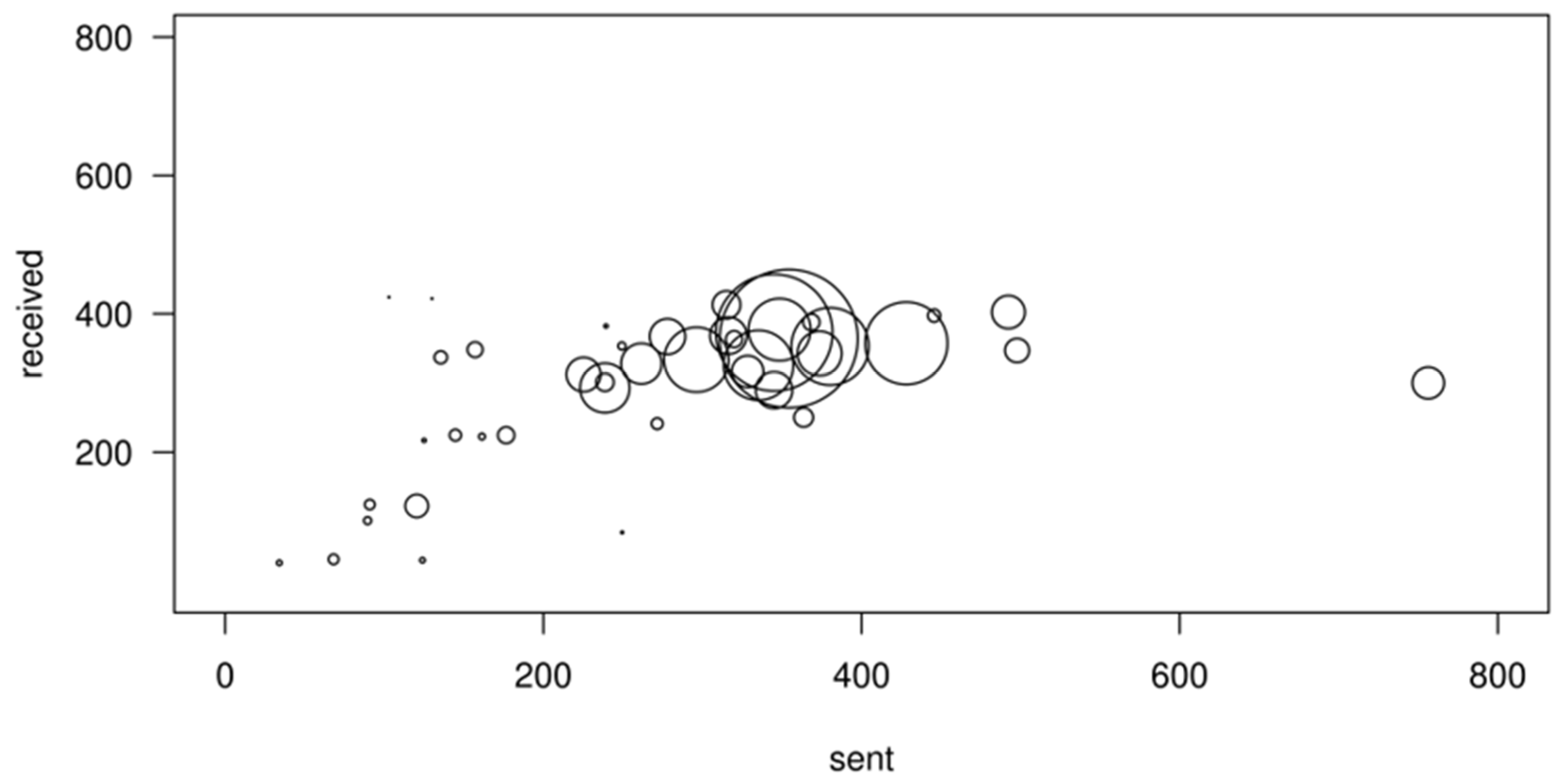
The correlation between the number of sent and received emails is even higher when summarized at department level (Pearson correlation = 0.967). The number of emails sent by a department’s members to members of other departments is proportional to the number of emails received from other departments. In addition, even though there is significant variance in the number of emails sent or received by each individual, the aggregate figures at department level are, to a large extent, proportional to the number of individuals in each department (Figure 2). Even though there is significant variance among individuals in regard to email activity, the email flows between departments is symmetrical.
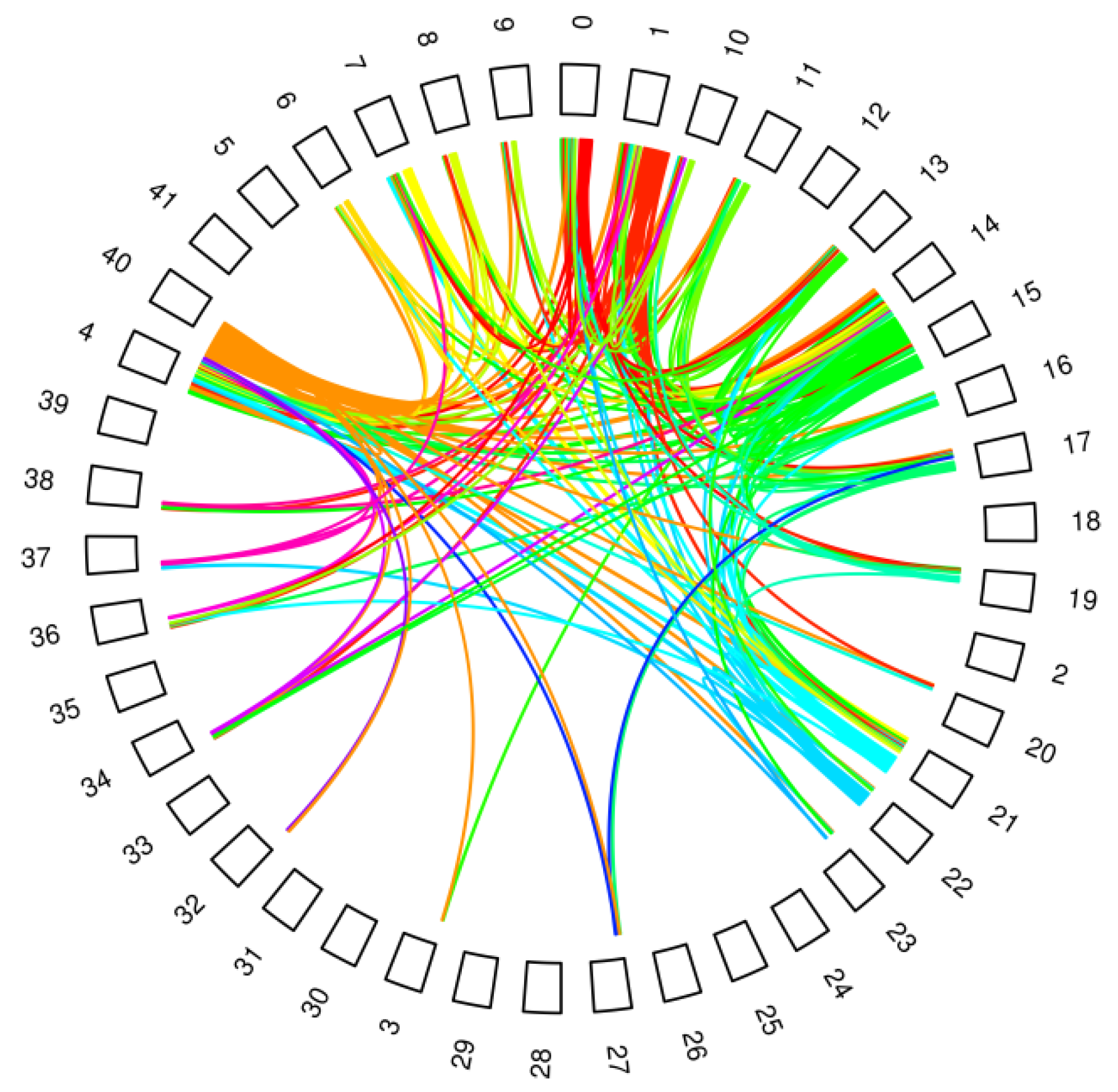
Given that the email traffic network has a high number of nodes and connections, it is practically impossible to visualize its structure in a meaningful way. Even when summarizing at department level, mapping the connections between the 42 nodes in order to identify patterns in the flow of information is still a complicated task. Figure 3 summarizes the top 10% of directional bilateral email flows between departments. While a few departments appear frequently in these bilateral flows, the pattern of connections implies that no department is dominant in terms of intra-institutional email traffic.
The basic statistics of email activity during the period comprise of the traffic data for the network at individual (Table 2) and department (Table 3) level. There is high variance in regard to the number of emails each member of the network sent or received during the period, as well as in the ratio between the two. There are a few members that dominate the institution in terms of the number of emails sent. Twenty members sent more than 2500 emails during the period, perhaps due to an information dissemination role that they may have. But sending many emails does not necessarily result in receiving many (or vice versa). Several different profiles seem to be present in the dataset, again, probably due to the different roles in the institution and the communication patterns each individual prefers.
4. Graph Theory Indicators
The basic traffic data across the network provides an overview of the activity but is not sufficient to explain the role of each individual in the organization. Graph theory indicators are commonly used in social network analysis in order to describe the topology of a network and explain the relationships among its members. The three most frequently used indicators address centrality, a measure of the importance of each individual (corresponding to a node in the network) within the social network: degree centrality, closeness centrality, and betweenness centrality. All three centrality indicators were introduced by Freeman in 1979 [28] and form the basis of current SNA methods.
Degree centrality is the simplest expression of centrality and corresponds to the total number of existing connections between an individual node and the other nodes of the network. If when a connection between nodes i and j exists, and in the opposite case, the basic definition of degree centrality is:
Normalizing the indicator adjusts for the network size by expressing a node’s centrality as a share of its maximum possible level, when connections with all other nodes in the system are present. If N the number of nodes in the network [29]:
For non-directed networks, is assumed. In most social networks, however, and particularly in the email network used here, connections are asymmetric, and is quite frequent in the flow of information. In such a case, the two variants of degree centrality assuming a directed graph may differ:
In practice, the degree centrality in a network of email flows coincides with the share of unique senders of emails received by each individual (in-degree) and the share of unique recipients of emails sent by each individual (out-degree).
Closeness centrality is an indicator of the centrality of each node based on the distance between each individual node and all other nodes in the network. It is calculated as the as the reciprocal of the sum of the length of the shortest paths between node i and all other nodes in the network [30]:
where is the distance (number of edges) between nodes i and j.
Normalization, in order to account for the network size, is performed by multiplying closeness by N − 1, where N is the number of nodes in the network. The two directional forms of closeness after this transformation correspond to the inverse of the average distance from each node [31]:
Betweenness centrality measures the number of shortest paths between all other nodes of the network that pass through an individual node. If is the number of all shortest paths between all other nodes in the network, and is the number of those shortest paths that pass through i, betweenness centrality is calculated as:
As in the case of the other centrality indicators, betweenness centrality can also account for different weights that express distance and differentiate between the directions of the connection. The general case, thus, can be transformed into:
The calculations of these standard centrality indicators for the reference email network used here were done with the igraph software package in [32]. The results for the main indicators are summarized in Table 4, with their standard and, where applicable, weighted and/or directional expressions.
Degree centrality is a direct reflection of the number of unique individuals within the network that an email was exchanged with. The basic expression, normalized but non-directional, does not distinguish between sending or receiving an email. On average, each individual has been in contact with (in the sense that an email was sent to or received from) 6.8% of the individuals in the network during the period covered (67 out of a total of 985). The reach of contacts ranges from a minimum of 0.03% (3 individuals) to close to 55% (540 individuals).
If the direction of the email flow is taken into account, the directional version of degree centrality allows more detail in the characterization of each node. The sum of the two directions of directed degree centrality equals the undirected degree centrality for each node. Nevertheless, the differences in the distribution of values reflect the asymmetry in the number of unique senders and respondents in the network and the varying patterns in email activity of individual members of the network. Degree centrality is positively skewed, with its distribution having a long tail towards values of high centrality. This is the result of a low number of nodes being highly central in terms of the number of individuals they exchanged emails with, either because they sent emails to a higher proportion of the network than the average (out-degree) or because they received proportionally more (in-degree). The skewness of out-degree centrality is significantly higher than that of –in-degree due to the dominant role of a few members as sender of emails.
The closeness centrality indicators reflect a certain degree of symmetry in regard to their distribution statistics. The average member of the network is equally close to the center, regardless of whether incoming or outgoing email flow is considered. However, closeness for outgoing emails has a lower standard deviation and higher skewness than for incoming emails. This probably signifies that the relatively few members who send emails to a large part of the network act as an efficient channel of information flow across the network. The mean values for closeness centrality in Table 4 correspond to an average distance of 2.654 edges for outgoing emails and 2.652 edges for incoming emails, confirming the observation that the email network analyzed here is dense and highly connected.
Betweenness centrality presents some small differences when the direction of the email flow is taken into account. While the two values are highly correlated at node level (Pearson correlation = 0.965), individuals with a large imbalance between the numbers of incoming and outgoing messages do have a marginal influence on the overall distribution.
5. Extending Clustering Approach
As described in Section 1, recent advances in SNA indicate the importance of identifying clusters of individuals and communities in social networks. A simplified approach may consider binary unidirectional connections between individuals. While such simplifications may not influence the overall analysis in certain types of social networks (e.g., club membership), they may distort the findings significantly in networks where the direction and intensity of information flow can be of major importance (e.g., Twitter, email or bibliographic network analysis). The local clustering coefficient was introduced in the seminal paper of Watts and Strogatz [14] as a measure to determine whether a graph is a small-world network by quantifying how close a node and its neighbors are to being a clique. The clustering coefficients are used here in order to explore the hypothesis that email networks present Small World characteristics. The underlying question is whether using such coefficients—and in particular their directional form—improves the understanding of the behavior of the members of the network.
The clustering coefficient of node i is equal to the number of triangles connected to this node divided by the number of triples (i.e., potential triangles) centered on it [14]:
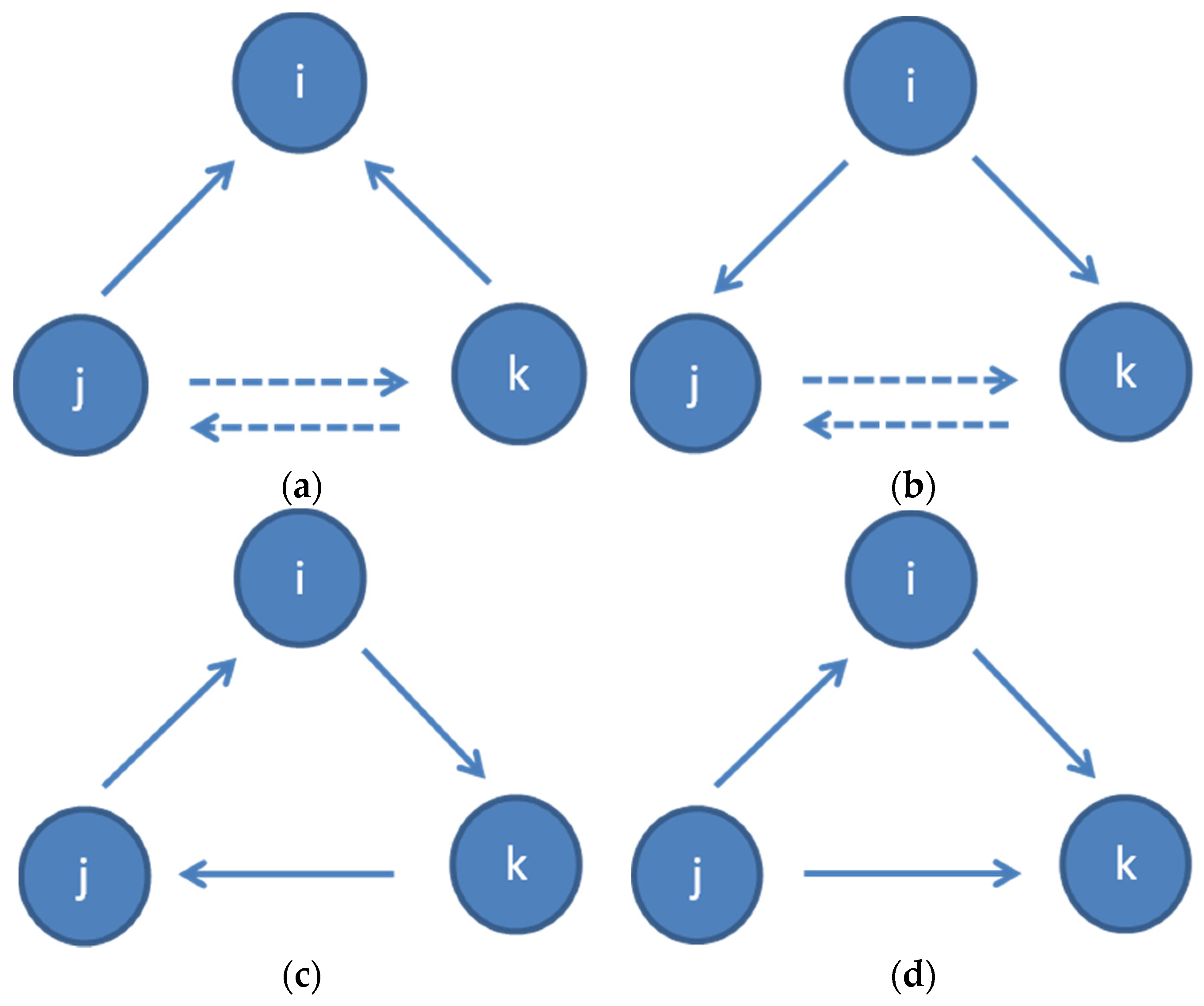
where is the number of triangles formed between node i and its possible neighbors, and is the degree of the node (the number of individual connections). Opsahl and Panzarasa (2009) [33] extended the definition of the clustering coefficient to weighted networks. Similar to the case of adding weights and direction to the standard centrality indicators in Section 4, assuming directed clustering in weighted networks can provide additional insight into the structure and dynamics of a social network. Nevertheless, a node can be part of triangles with arcs pointing in different directions. Four types of triangles can be distinguished [11,13]:
- Cycle: a triangle where every arc has the same direction (j→i, i→k, k→ j or vice versa) (Figure 4c); and
- Middleman: a triangle where the two arcs of i have different directions and there is an arc between j and k (or vice versa), without forming a cycle. There are two arcs incoming to k or j (j→i, i→k, j→k or vice versa) (Figure 4d).
A directed clustering coefficient can be specified for each of the above cases, in order to account for the different patterns. Each coefficient is defined as the number of triangles of i with a specific pattern of arc directions, divided by the number of potential specific triangles of i.
If a binary variable to indicate whether there is a connection between i and j or not, and is the number of emails sent from i to j (and, consequently, if and only if ), the four clustering coefficients can be defined as:
where is the strength of the connection between node i and its adjacent nodes j, expressed as:
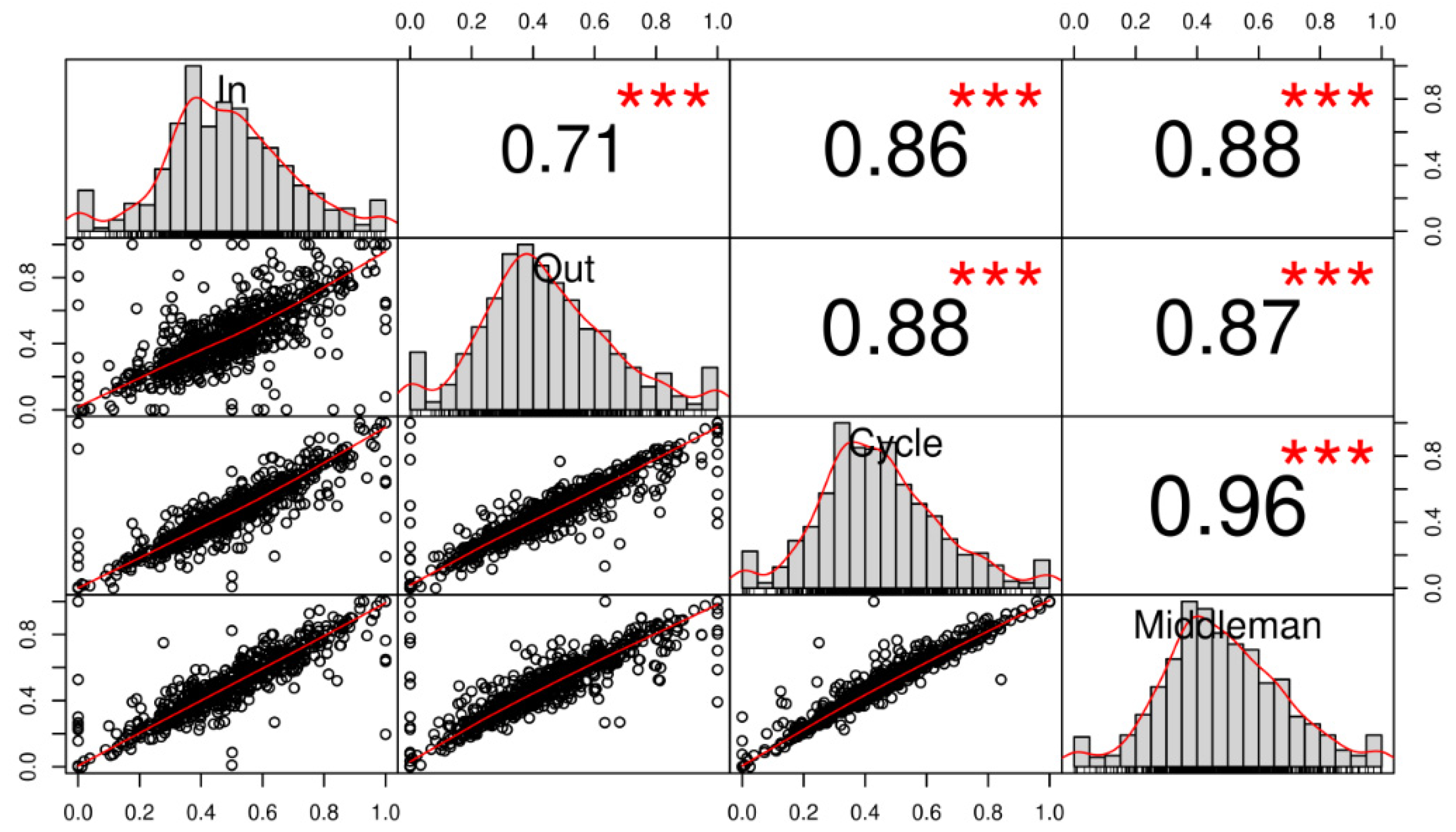
The clustering coefficients were calculated with the DirectClustering package, are summarized in Table 5, and are visualized in Figure 5. An in-clustering coefficient with a value of 1 corresponds to the cases of individuals who were on the receiving side in all triangles formed by their email exchanges. This was the case for 14 individuals in the sample. The mean of the indicators ranges from 0.4413 to 0.4828. Variation appears to be higher for the In- and Out-coefficient than for the Cycle and Middleman. In terms of skewness, Out- and Cycle coefficients have a higher value. The four coefficients present a high level of correlation, which is to a certain degree expected. The majority of the individual members of the network would participate in various forms of triangles with different directions and intensities of email flow. The number of emails sent to an individual is also highly correlated with the number of emails received from the same individual, and, consequently, the indicators weighted on the intensity of the bilateral connections will inherit the correlation. The high correlation levels can be useful in pattern analysis, especially in cases of networks where one would expect uniform distributions. The outliers can provide significant information about their role in the organization or identify a behavior that is not expected. Especially in regard to the relation between the In- and Out-clustering coefficients, the explanation of the part of their relation that is not explained by collinearity may be useful in identifying individual or organizational patterns. For example, a high in-clustering coefficient may signify the individual’s role as a transmitter of information from the local cluster to the rest of the system. If the same individual has a low out-clustering coefficient, the flow of information in the opposite direction (from the rest of the system to the local cluster) is more limited. Depending on the case, this may be the result of the hierarchical structure of the local cluster (i.e., the individual is the manager of the team formed by several triangles) or a symptom of imbalances in the flow of communication. In practical terms, the graphical representation of the correlation between the four clustering coefficients (Figure 5) facilitates the identification of outliers.
6. Symmetrical and A-Symmetrical Models
Having presented the differences between symmetrical and directed indicators, the question can be transformed into whether using one or the other type of indicators influences the quality of the analysis of patterns in a social network. An experiment can be made by using a variable that expresses an operational characteristic of the network—independent from its topology—and estimate how the various centrality and clustering coefficients explain its variation. Given the data available in this dataset, a suitable variable that is independent from the individual network measures is the reaction time to emails. The dataset provides the timestamp for each email, information that was not used in the calculations of the indicators in the previous sections. While the reaction time between emails does not necessarily correspond to the time that has passed for a specific email to be responded, it still provides a quantifiable indicator of the temporal dimension of the email interaction between two members of a social network. Shinkuma et al. [34] suggest that the frequency of interaction can be used as an indicator to characterize interpersonal communication in the network graphs.
In the experiment used here, a new indicator is constructed based on the email timestamps included in the dataset. If only the email exchanges that were bilateral during the period covered by the dataset (i.e., ) are taken into account and on the premise that the timestamp difference in an email exchange between two individuals is a proxy of the response time, the exchange of emails between i and j would have the form of a series that can be ordered by time.
The series would have n elements, where n is the number of emails between i and j, regardless of direction. The number of emails from i to j would be equal to k, where k < n. Each email has a timestamp {tn > tn−1}.
The response times of i to the emails sent by j can be calculated as the difference between the timestamp of each email and the last unanswered email :
The timestamp of the last unanswered email would correspond to the timestamp of the latest email :
In a similar fashion, the response times by j to emails sent by I can be calculated as the difference between the timestamps of each sent email and the next received email , if any:
The timestamp of the next email would be that of the first email received after each :
An example of the calculation of response times is given in Table 6.
The average time of response by an individual i would be:
while the average speed of responses received would be:
The average speed of reply is, however, very sensitive to the period of analysis used and to the specific day or hour that a specific email was sent. A more suitable indicator of the relative importance of an individual in the network could be the share of outgoing emails that were responded within a certain time threshold.
The formulation that calculates the share of responses in the opposite direction within the threshold can be used as an indicator of an individual’s own average speed of response.
Two different indicators are tested, with a 7 d and a 24 h threshold, respectively. For each indicator, three different models that explain the variation were developed:
- Conventional model: independent variables include main statistics on individual email activity (number of emails sent and share of own replies within the threshold period) and standard symmetric centrality indicators;
- Clustering model: independent variables include main statistics on individual email activity and directed clustering indicators; and
- Extended Directional model: independent variables combine main statistics on individual email activity, directed centrality indicators, and directed clustering indicators.
6.1. Share of Outgoing Emails Responded Within 7 Days
The comparison of the three models that use a 7 d threshold is summarized in Table 7. The main statistics indicators that are significant in all three models are the number of emails sent () and the individual’s own speed in replying (). This suggests that there is a high degree of reciprocity in an individual’s email activity. The individuals in the network examined here who sent more emails, on average, received faster responses. At the same time, the individuals who reply fast have their emails also replied to fast. Both variables suggest that the more active the role of the individual is in the system, the stronger the role is that the individual has in the network (at least as far as the dependent variable expresses such strength). Of course, it is possible that the causal relationship has the opposite direction, i.e., the faster that an individual’s emails are responded, the higher the number and faster the responses of the individual.
The conventional model uses the two variables above and the individual’s closeness centrality indicator. The relation is positive, meaning that, the closer the individual is to the center of the network, the higher the share of the individual’s emails that are responded within 7 d. Neither degree nor betweenness appear as significant variables, suggesting that the speed of replies is not a function of the number of individual connections nor of the number of shortest paths that an individual node forms part of.
The clustering model, which uses the directed clustering coefficients, suggests that three directed coefficients can be useful in interpreting an individual’s role in the network. There is a correlation with both the In- and Out-clustering coefficient and a negative correlation with the cycle clustering coefficient. This indicates that the participation in triads which have all three nodes communicating with each other tend to have a more active role in the overall network. Conversely, if the individual acts simply as a middleman, i.e., is part of the weaker communication channel in a triad, the individual’s role in the network tend to be less active, at least measured in terms of the time for emails to be responded.
The Extended Directional model combines centrality and clustering indicators accounting, in both cases, for direction and weights. This model maintains the main independent variables of the other two approaches, rebalancing their respective estimates and resulting in a visible improvement in accuracy. The R2 coefficient of the Extended Directional model is 0.8596 compared to 0.8468 and 0.8428 for the other two models, respectively. Closeness is considered in its directional version, which results in its weight in the model to be split in two. The two directions are not symmetrical though, with the in-closeness centrality having a negative correlation which roughly counter-balances the positive impact of the out-closeness one. The three clustering coefficients remain significant in the Extended Directional model, maintaining the direction of the influence, with small changes in the estimates. The estimates of In- and Out-clustering coefficients converge to comparable levels, while the estimate for the Middleman coefficient decreases further.
The difference when direction and weights are taken into account to explain variation is noticeable, and the accuracy of the model increases. The department that each individual belongs to does not appear as significant. The three standard graph theory indicators, Degree, Closeness, and Betweenness, appear to be inter-related, even in their directed version, and, consequently, only Closeness appears as significant.
6.2. Share of Outgoing Emails Responded Within 24 Hours
A second set of models that use a threshold of 24 h for the delay in responses is summarized in Table 8. All three models have a lower accuracy than their corresponding version that uses 7 d as a threshold. This is probably a result of the time scale used, since counting the delay this way would include weekends and distort the speed in response. Even so, this threshold is useful for confirming the robustness of the approach. All independent variables for all three model configurations present the same direction in their impact on the dependent variable, with estimates having the same order of magnitude and showing a comparable level of statistical significance.
The reciprocity in the speed of responses remains. Individuals who respond within 24 h have a higher probability of their emails being responded within 24 h. High activity in terms of the number of emails sent is again an important indicator. The opposite directions of the estimates for the two directional closeness centrality indicators confirms the observation made in the 7 d model, i.e., that out-closeness is positively correlated with speed of responses received, while in-closeness has the contrary effect. The In-, Out-, and Middleman clustering coefficients also corroborate the results of the 7 d model.
The results of the two models are robust enough to allow a generalization of the interpretation of each variable. The individual’s own activity in terms of number, frequency, and destination of emails appears to reflect the relative importance of the individual in the network expressed as the share of timely responses to an individual’s email within either a 7 d or 24 h period. In terms of activity, the frequency and response delay of the individual’s own emails are a determinant of how others respond. The higher the number of emails sent and the faster emails are replied by an individual, the faster the responses of the individual’s correspondents can be expected to be. From a topology perspective, taking into account the asymmetry of closeness centrality allows a more detailed evaluation of its impact. A central role as an emitter of information (high Out-closeness) increases the probability of quick reactions by others. In the opposite case, simply being close to the center as receiver of information (high Out-closeness) decreases this probability. Small world aspects can also explain part of the role. The middleman clustering coefficient has a clearly negative correlation with response time, something that suggests that there is a correspondence with the importance of an individual’s role in the system. In-clustering and out-clustering both have a positive correlation, possibly indicating that the individuals with high coefficients are a link between local clusters and the rest of the system.
6.3. Validation of Methodology on Alternative Datasets
The methodology presented here appears to applicable in the case of the reference email network, providing results that, to a certain extent, allow some insights on the structure and dynamics of the organization. A question, though, is whether this approach can be generalized to other type of networks, either of email or other social network activity. In order to test the robustness of the approach, the models developed using the email-Eu-core-temporal network (Section 6.1 and Section 6.2) are applied on two different validation networks. The first validation network is “CollegeMsg”, a dataset of private messages sent on an online social network at the University of California, Irvine, originally used in Reference [35]. Users could search the network for others and then initiate conversation based on profile information. The dataset consists of 59,835 messages among the 1899 members. It includes the anonymized identity of the sender and recipient, as well as the timestamp of the message. The timespan of the dataset is 193 days and permits the calculation of response times. Compared to the email-Eu-core-temporal dataset (330 thousand emails between 986 members, over 18 months), CollegeMsg is less dense and has a shorter timespan. In addition, the dynamics of participating in a message board differ from that of an email network in term of speed, frequency, and intensity of interaction between members.
The second dataset used for validation is the Enron email network [36]. It consists of 52,587 nodes and 517,399 emails, in a timespan of more than four years. The dataset is not limited to Enron employees but covers all email exchanges with an Enron employee as a sender or recipient. On the other hand, there is no information available on the hierarchical structure inside Enron, since only email addresses are included. As a result, while it is a much larger dataset than both email-Eu-core-temporal and CollegeMsg, it is less dense and has a longer timespan than both.
Table 9 summarizes the fit for the 7 d and 1 d responses applied on each of the three datasets. In all three cases, the extended directional model explains variation better than either the conventional or the clustering model. The fit for the smallest dataset (CollegeMsg) is better for both the timescales used and in all three model variations. In contrast, the large Enron dataset has a lower (though still acceptable) R2 but also demonstrates a visible improvement when the Extended Directional model is applied. It is also notable that the 1 d timescale has a better fit than the 7 d timescale in the case of Enron. This comparison confirms that the explanatory power of the model increases in all cases when directional coefficients are used. The overall accuracy, though, depends on the specificities of each network. Different parameters, especially in regard to the timescale used, would probably improve the results of the comparison.
Table 10 compares the estimates for each variable used in the extended directional model for each dataset. The main observations made in the analysis of the email-Eu-core-temporal network still hold true. The users own activity in terms of number of emails and own time to respond explains a large part of variation. The estimates for in- and out-closeness normally have opposite signs, as do the ones for in- and out-clustering. The results of the validation suggest that the main principles of the methodology presented here are still valid. Directional indicators, including the Small World indicators, do add value to the information and improve the predictive models in both alternative networks tested.
The detailed results for the two validation networks can be found in the Appendix A.
7. Conclusions
The work presented here addressed options to improve current practice in Social Network Analysis (SNA). The main novelty of the approach proposed is two-fold. The introduction of weighted and directed indicators in standard SNA adds useful information on the direction of intensity of social network interactions. In addition, the application of small world directional clustering coefficients improves interpretability. The experiments using a reference email network demonstrate that taking into account the direction and weights of the social network connections can improve the understanding of the network patterns and operational aspects.
The results also suggest that a hitherto perceived complication of social network—the lack of symmetry—can, in fact, be seen as an advantage. Directed and weighted cluster coefficients may explain part of the variance in email activity, which is a promising candidate for explaining an individual’s role within an organization. In addition, the significance of the local clustering coefficients in all experiments with the three different social networks confirms the hypothesis that email networks present certain Small World elements.
While the method and indicators were tested only on three networks, it is probably applicable to other types of social networks, regardless of scale and structure. Most social networks entail asymmetries in the flow of information and the relation between its members. The results presented here suggest that there is a correlation between this asymmetry and the role of each member in the network, an observation that can be probably extended to other social networks.
The approach obviously has several limitations that should be kept in mind when interpreting the results. The specific data used are a snapshot for a specific period in time. Most probably, the patterns of social network activity change over time either due to the own network’s dynamics or as a result of the introduction of alternative social networks. In the case of emails, the gradual introduction of competitive communication tools, such as intranet or instant messaging, may modify the importance of this channel of communication. Another major caveat is the lack of objective evaluations of an individual’s role so that a model that correlates it to SNA indicators can be developed and validated. This is, however, a general weakness of SNA-based analysis, since it is seldom possible to demonstrate a causal relationship between social network activity and a real life assessment of an individual’s importance.
The improvements proposed here, but also the limitations that were identified, signify the need to extend research on social network analysis and organizational dynamics. More social network data will be probably available for research in the future, providing an opportunity for the often purely theoretical approaches to be further developed and tested.
Funding
This research received no external funding.
Conflicts of Interest
The author declares no conflict of interest.
Appendix A. Results for Validation Networks

Table A1.
College dataset, 7-day model.
| Conventional | Clustering | Extended Directional | ||||
|---|---|---|---|---|---|---|
| Estimate | Pr(>|t|) | Estimate | Pr(>|t|) | Estimate | Pr(>|t|) | |
| Number of emails sent | −1.113 × 10⁻⁴ | 0.00601 ** | 1.403 × 10⁻⁴ | 0.000995 *** | −8.578 × 10⁻⁶ | 0.87386 |
| Share of own replies within period | 9.635 × 10⁻² | 0.04899 * | 9.553 × 10⁻¹ | <2 × 10⁻¹⁶ *** | 9.887 × 10⁻² | 0.04459 * |
| Closeness | 2.949 | <2 × 10⁻¹⁶ *** | ||||
| Closeness (in) | 4.887 × 10⁻² | 0.21796 | ||||
| Closeness (out) | −2.439 | 0.20323 | ||||
| “In” clustering coefficient | 1.245 × 10⁻¹ | 0.004622 ** | 4.887 × 10⁻² | 0.21796 | ||
| “Out” clustering coefficient | 4.702 × 10⁻³ | 0.878011 | −2.164 × 10⁻² | 0.43262 | ||
| “Middleman” clustering coefficient | −4.740 × 10⁻² | 0.272049 | −1.180 × 10⁻² | 0.76112 | ||
| Adjusted R-squared | 0.9823 | 0.9781 | 0.9823 | |||
| p-value | <2.2 × 10⁻¹⁶ | <2.2 × 10⁻¹⁶ | <2.2 × 10⁻¹⁶ | |||
Significance codes: 0 ‘***’ 0.001 ‘**’ 0.01 ‘*’ 0.05 ‘.’ 0.1 ‘ ’ 1.
Table A2.
College dataset, 1-day model.
| Conventional | Clustering | Extended Directional | ||||
|---|---|---|---|---|---|---|
| Estimate | Pr(>|t|) | Estimate | Pr(>|t|) | Estimate | Pr(>|t|) | |
| Number of emails sent | −9.079 × 10⁻⁵ | 0.085. | 2.369 × 10⁻⁴ | 0.000206 *** | 7.396 × 10⁻⁵ | 0.30228 |
| Share of own replies within period | 1.813 × 10⁻¹ | 3.69 × 10⁻¹⁰ *** | 9.111 × 10⁻¹ | <2 × 10⁻¹⁶ *** | 1.866 × 10⁻¹ | 1.04 × 10⁻¹⁰ *** |
| Closeness | 2.396 | <2 × 10⁻¹⁶ *** | ||||
| Closeness (in) | 8.495 | 0.00103 ** | ||||
| Closeness (out) | −6.139 | 0.01784 * | ||||
| “In” clustering coefficient | 1.529 × 10⁻¹ | 0.020532 * | 4.493 × 10⁻² | 0.40060 | ||
| “Out” clustering coefficient | −1.161 × 10⁻¹ | 0.011989 * | −9.589 × 10⁻² | 0.01030 * | ||
| “Middleman” clustering coefficient | 8.458 × 10⁻² | 0.192056 | 4.440 × 10⁻² | 0.39701 | ||
| Adjusted R-squared | 0.9607 | 0.9404 | 0.9611 | |||
| p-value | <2.2 × 10⁻¹⁶ | <2.2 × 10⁻¹⁶ | <2.2 × 10⁻¹⁶ | |||
Significance codes: 0 ‘***’ 0.001 ‘**’ 0.01 ‘*’ 0.05 ‘.’ 0.1 ‘ ’ 1.
Table A3.
Enron dataset, 7-day model.
| Conventional | Clustering | Extended Directional | ||||
|---|---|---|---|---|---|---|
| Estimate | Pr(>|t|) | Estimate | Pr(>|t|) | Estimate | Pr(>|t|) | |
| Number of emails sent | 2.161 × 10⁻⁵ | 0.462 | 1.245 × 10⁻⁴ | 6.72 × 10⁻⁵ *** | 1.413 × 10⁻⁵ | 0.742 |
| Share of own replies within period | 4.322 × 10⁻² | 4.481 × 10⁻² | 5.021 × 10⁻¹ | <2 × 10⁻¹⁶ *** | 3.915 × 10⁻² | 0.384 |
| Closeness | 1.482 | 1.201 × 10⁻¹ | ||||
| Closeness (in) | −1.107 × 101 | 0.881 | ||||
| Closeness (out) | 1.262 × 101 | 0.865 | ||||
| “In” clustering coefficient | 3.834 × 10⁻² | 0.521 | −1.115 × 10⁻¹ | 0.046 * | ||
| “Out” clustering coefficient | 1.761 × 10⁻¹ | 0.145 | 8.092 × 10⁻² | 0.461 | ||
| “Middleman” clustering coefficient | 7.172 × 10⁻² | 0.644 | 3.361 × 10⁻² | 0.739 | ||
| Adjusted R-squared | 0.6082 | 0.5239 | 0.6091 | |||
| p-value | <2.2 × 10⁻¹⁶ | <2.2 × 10⁻¹⁶ | <2.2 × 10⁻¹⁶ | |||
Significance codes: 0 ‘***’ 0.001 ‘**’ 0.01 ‘*’ 0.05 ‘.’ 0.1 ‘ ’ 1.
Table A4.
Enron dataset, 1-day model.
| Conventional | Clustering | Extended Directional | ||||
|---|---|---|---|---|---|---|
| Estimate | Pr(>|t|) | Estimate | Pr(>|t|) | Estimate | Pr(>|t|) | |
| Number of emails sent | 1.154 × 10⁻⁵ | 8.94 × 10⁻⁶ *** | 1.208 × 10⁻⁵ | 1.69 × 10⁻⁶ *** | 3.523 × 10⁻⁶ | 0.35463 |
| Share of own replies within period | 6.126 × 10⁻¹ | <2 × 10⁻¹⁶ *** | 6.149 × 10⁻¹ | <2 × 10⁻¹⁶ *** | 6.110 × 10⁻¹ | <2 × 10⁻¹⁶ *** |
| Closeness | 3.245 × 10⁻³ | 0.492 | ||||
| Closeness (in) | −1.847 × 101 | 0.00524 ** | ||||
| Closeness (out) | 1.847 × 101 | 0.00522 ** | ||||
| “In” clustering coefficient | −2.139 × 10⁻⁴ | 0.964 | −3.092 × 10⁻³ | 0.53343 | ||
| “Out” clustering coefficient | 1.449 × 10⁻³ | 0.883 | 1.779 × 10⁻³ | 0.85563 | ||
| “Middleman” clustering coefficient | −1.584 × 10⁻³ | 0.860 | −2.073 × 10⁻³ | 0.81785 | ||
| Adjusted R-squared | 0.6791 | 0.678 | 0.6814 | |||
| p-value | <2.2 × 10⁻¹⁶ | <2.2 × 10⁻¹⁶ | <2.2 × 10⁻¹⁶ | |||
Significance codes: 0 ‘***’ 0.001 ‘**’ 0.01 ‘*’ 0.05 ‘.’ 0.1 ‘ ’ 1.
References
- Zhong, S.; Geng, Y.; Liu, W.; Gao, C.; Chen, W. A bibliometric review on natural resource accounting during 1995–2014. J. Clean. Prod. 2016, 139, 122–132. [Google Scholar] [CrossRef]
- Christodoulou, A.; Christidis, P. Measuring cross-border road accessibility in the European Union. Sustainability 2019, 11, 4000. [Google Scholar] [CrossRef] [Green Version]
- Kim, J.; Hastak, M. Social network analysis: Characteristics of online social networks after a disaster. Int. J. Inf. Manag. 2018, 38, 86–96. [Google Scholar] [CrossRef]
- De Mesa, E.G.; Hidalgo, I.; Christidis, P.; Ciscar, J.C.; Vegas, E.; Ibarreta, D. Modeling the impact of genetic screening technologies on healthcare: Theoretical model for asthma in children. Mol. Diagn. Ther. 2007, 11, 313–323. [Google Scholar] [CrossRef] [PubMed]
- Christidis, P. Four shades of Open Skies: European Union and four main external partners. J. Transp. Geogr. 2016, 50, 105–114. [Google Scholar] [CrossRef]
- Pan, Y.; Tan, W.; Chen, Y. The analysis of key nodes in complex social networks, Lecture Notes in Computer Science (including subseries Lecture Notes in Artificial Intelligence and Lecture Notes in Bioinformatics). LNCS 2017, 10603, 829–836. [Google Scholar]
- Christidis, P.; Losada, A.G. Email based institutional network analysis: Applications and risks. Soc. Sci. 2019, 8, 306. [Google Scholar] [CrossRef] [Green Version]
- Lazer, D.; Pentland, A.; Adamic, L.; Aral, S.; Barabasi, A.L.; Brewer, D.; Christakis, N.; Contractor, N.; Fowler, J.; Myron, G.; et al. Social science: Computational social science. Science 2009, 323, 721–723. [Google Scholar] [CrossRef] [Green Version]
- Benson, A.R.; Gleich, D.F.; Leskovec, J. Higher-order organization of complex networks. Science 2016, 353, 163–166. [Google Scholar] [CrossRef] [Green Version]
- Clemente, G.P.; Grassi, R. Directed clustering in weighted networks: A new perspective. Chaos Solitons Fractals 2018, 107, 26–38. [Google Scholar] [CrossRef] [Green Version]
- Clemente, G.P.; Grassi, R. Directed Weighted Clustering Coefficient (Package ‘DirectedClustering’). 2018. Available online: https://cran.r-project.org/web/packages/DirectedClustering/DirectedClustering.pdf (accessed on 31 March 2020).
- Adamic, L.A.; Adar, E. Friends and neighbors on the web. Soc. Netw. 2001, 25, 211–230. [Google Scholar] [CrossRef] [Green Version]
- Barrat, A.; Barthelemy, M.; Pastor-Satorras, R.; Vespignani, A. The architecture of complex weighted networks. Proc. Natl. Acad. Sci. USA 2004, 101, 3747. [Google Scholar] [CrossRef] [PubMed] [Green Version]
- Watts, D.; Strogatz, S. Collective dynamics of ‘small-world’ networks. Nature 1998, 393, 440–442. [Google Scholar] [CrossRef] [PubMed]
- Fagiolo, G. Clustering in complex directed networks. Phys. Rev. E 2007, 76, 026107. [Google Scholar] [CrossRef] [PubMed] [Green Version]
- Fagiolo, G.; Reyes, J.; Schiavo, S. World-trade web: Topological properties, dynamics, and evolution, Physical Review E—Statistical. Phys. Rev. E Stat. Nonlin. Soft Matter Phys. 2008, 79, 036115. [Google Scholar]
- Traud, A.L.; Mucha, P.J.; Porter, M.A. Social structure of Facebook networks. Phys. A 2012, 391, 4165–4180. [Google Scholar] [CrossRef] [Green Version]
- Chen, D.B.; Gao, H.; Lü, L.; Zhou, T. Identifying influential nodes in large-scale directed networks: The role of clustering. PLoS ONE 2013, 8, 0077455. [Google Scholar] [CrossRef] [Green Version]
- Myers, S.A.; Sharma, A.; Gupta, P.; Lin, J. Information network or social network? The structure of the twitter follow graph, WWW 2014 Companion. In Proceedings of the 23rd International Conference on World Wide Web, Seoul, Korea, 7–11 April 2014; pp. 493–498. [Google Scholar]
- Hangal, S.; MacLean, D.; Lam, M.; Heer, J. All Friends are Not Equal: Using Weights in Social Graphs to Improve Search. In Proceedings of the Fourth ACM Workshop on Social Network Mining and Analysis Held in Conjunction with ACM SIGKDD International Conference on Knowledge Discovery and Data Mining (KDD), Washington, DC, USA, 24–28 July 2010. [Google Scholar]
- Portela, J.; Villalba, L.J.G.; Silva Trujillo, A.G.; Sandoval Orozco, A.L.; Kim, T.-H. Estimation of anonymous email network characteristics through statistical disclosure attacks. Sensors 2016, 16, 1832. [Google Scholar] [CrossRef]
- Chen, Q.; Su, H.; Liu, J.; Yan, B.; Zheng, H.; Zhao, H. In Pursuit of social capital: Upgrading social circle through edge rewiring. Web Big Data 2019. [Google Scholar] [CrossRef]
- Tang, J.; Lou, T.; Kleinberg, J. Inferring social ties across heterogenous networks. In Proceedings of the Fifth ACM International Conference on Web Search and Data Mining, ACM, Washington, DC, USA, 8–12 February 2012; pp. 743–752. [Google Scholar]
- Chen, R. Living a private life in public social networks: An exploration of member self-disclosure. Decis. Support Syst. 2013, 55, 661–668. [Google Scholar] [CrossRef]
- Saqr, M.; Fors, U.; Nouri, J. Using social network analysis to understand online problem-based learning and predict performance. PLoS ONE 2018, 13, e0203590. [Google Scholar] [CrossRef] [PubMed] [Green Version]
- Yin, H.; Benson, A.R.; Leskovec, J.; Gleich, D.F. Local Higher-order Graph Clustering. In Proceedings of the 23rd ACM SIGKDD International Conference on Knowledge Discovery and Data Mining, New York, NY, USA, 13–17 August 2017. [Google Scholar]
- Leskovec, J.; Kleinberg, J.; Faloutsos, C. Graph Evolution: Densification and Shrinking Diameters. Acm Tkdd 2007, 1, 2-es. [Google Scholar] [CrossRef]
- Freeman, L.C. Centrality in networks: I. Conceptual clarification. Soc. Netw. 1979, 1, 215–239. [Google Scholar] [CrossRef] [Green Version]
- Marsden, P. Measures of Network Centrality. In International Encyclopedia of the Social & Behavioral Sciences, 2nd ed.; Elsevier: Amsterdam, The Netherlands, 2015; pp. 532–539. [Google Scholar]
- Bavelas, A. Communication patterns in task-oriented groups. J. Acoust. Soc. Am. 1950, 22, 725–730. [Google Scholar] [CrossRef]
- Marchiori, M.; Latora, V. Harmony in the small-world. Phys. A 2000, 285, 539–546. [Google Scholar] [CrossRef] [Green Version]
- Csardi, G.; Nepusz, T. The igraph software package for complex network research. Int. J. Complex Syst. 2006, 1695, 1–9. [Google Scholar]
- Opsahl, T.; Panzarasa, P. Clustering in Weighted Networks. Soc. Netw. 2009, 31, 155–163. [Google Scholar] [CrossRef]
- Shinkuma, R.; Sugimoto, Y.; Inagaki, Y. Weighted network graph for interpersonal communication with temporal regularity. Soft Comput. 2019, 23, 3037–3051. [Google Scholar] [CrossRef] [Green Version]
- Panzarasa, P.; Opsahl, T.; Carley, K. Patterns and dynamics of users’ behavior and interaction: Network analysis of an online community. J. Am. Soc. Inf. Sci. Technol. 2009, 60, 911–932. [Google Scholar] [CrossRef]
- Klimmt, B.; Yang, Y. Introducing the Enron Corpus, CEAS Conference. 2004. Available online: http://ceas.cc/2004/168.pdf (accessed on 31 March 2020).
Figure 1.
Number of emails sent and received by each individual; color represents the department the individual belong to (logarithmic scale).
Figure 1.
Number of emails sent and received by each individual; color represents the department the individual belong to (logarithmic scale).

Figure 2.
Average number of emails sent and received per person for each department (bubble size is proportional to the number of department members).
Figure 2.
Average number of emails sent and received per person for each department (bubble size is proportional to the number of department members).

Figure 3.
Email traffic between departments (top 10% of bilateral traffic); each color represents a different sender department.
Figure 3.
Email traffic between departments (top 10% of bilateral traffic); each color represents a different sender department.

Figure 4.
Possible triangles in directed clustering coefficient analysis: (a) In, (b) Out, (c) Cycle, (d) Middleman.
Figure 4.
Possible triangles in directed clustering coefficient analysis: (a) In, (b) Out, (c) Cycle, (d) Middleman.

Figure 5.
Correlation matrix of clustering coefficients.

Table 1.
Comparison of related literature with present work.
| Authors | Network | Indicators | Directed | Weights |
|---|---|---|---|---|
| Adamic and Adar (2001) [12] | Web page network | Structural | Yes | Structural (number of links) |
| Watts and Strogatz (1998) [14] | Biological network; Collaboration network | Clustering | No | No |
| Barrat et al. (2004) [13] | Aviation network | Structural; Activity | yes | Activity (available seats per year) |
| Fagiolo (2007) [15] | International trade network | Clustering | Yes | Clustering (unweighted local coefficients) |
| Fagiolo et al. (2008) [16] | International trade network | Structural; Activity; Clustering | Yes | Clustering (weighted local coefficients) |
| Hangal et al. (2010) | Bibliography network; Twitter retweet network | Structural; Activity | Yes | Activity (directed influence between nodes) |
| Traud et al. (2012) [17] | Facebook contacts network | Structural; Clustering | No | No |
| Chen et al. (2013) [18] | Online community network; collaboration network | Clustering | Yes | Clustering (in- and out-degree) |
| Myers et al. (2014) [19] | Twitter follow graph | Structural; Clustering | Yes | No |
| Clemente and Grassi (2018) [11] | Theoretical graphs | Clustering | Yes | Clustering (weighted local coefficients) |
| Portela et al. (2016) [21] | email network | Structural; Clustering | Yes | No |
| Chen et al. (2019) [22] | email network | Structural | Yes | No |
| This work | email network | Structural; Activity; Clustering | Yes | Clustering (weighted local coefficients, based on References [21,22]) |
Table 2.
Basic email activity indicators, individual level.
| Indicator | Median | Mean | Minimum | Maximum | Standard Deviation | Skewness |
|---|---|---|---|---|---|---|
| Number of sent emails | 77 | 330.7 | 0 | 9782 | 740.4 | 5.43 |
| Number of received emails | 130 | 330.7 | 0 | 4710 | 483.9 | 2.88 |
| Ratio of number of sent to number of received emails | 0.767 | 1.553 | 0.002 | 303.6 | 11.43 | 25.11 |
Table 3.
Basic email activity indicators, department level.
| Indicator | Median | Mean | Minimum | Maximum | Standard Deviation | Skewness |
|---|---|---|---|---|---|---|
| Number of sent emails per person | 378.75 | 370.67 | 43.33 | 970.47 | 197.69 | 0.85 |
| Number of received emails per person | 423 | 392.63 | 52.67 | 640 | 146.89 | −0.61 |
| Ratio of number of sent to number of received emails | 0.90 | 1.02 | 0.24 | 2.88 | 0.552 | 1.8 |
Table 4.
Main statistics for graph theory indicators.
| Median | Mean | Minimum | Maximum | Standard Deviation | Skewness | |
|---|---|---|---|---|---|---|
| Degree centrality | 0.0478 | 0.0657 | 0.0020 | 0.5483 | 0.0623 | 2.34 |
| Degree centrality (in) | 0.0244 | 0.0322 | 0.0010 | 0.2116 | 0.0287 | 1.98 |
| Degree centrality (out) | 0.0234 | 0.0336 | 0.0010 | 0.3367 | 0.0349 | 2.72 |
| Closeness centrality | 0.3759 | 0.3787 | 0.3699 | 0.4692 | 0.0091 | 3.18 |
| Closeness centrality (in) | 0.3752 | 0.3779 | 0.3699 | 0.4692 | 0.0073 | 2.19 |
| Closeness centrality (out) | 0.3755 | 0.3775 | 0.3699 | 0.4265 | 0.0091 | 3.30 |
| Betweenness centrality | 958 | 2453.9 | 0 | 42,250 | 4449.6 | 4.40 |
| Betweenness centrality (directional) | 956 | 2446.6 | 0 | 42,225 | 4437.5 | 4.41 |
Table 5.
Main statistics for clustering coefficients.
| Clustering Coefficient | Median | Mean | Minimum | Maximum | Standard Deviation | Skewness |
|---|---|---|---|---|---|---|
| In | 0.4738 | 0.4828 | 0 | 1 | 0.2026 | 0.1466 |
| Out | 0.4167 | 0.4413 | 0 | 1 | 0.2141 | 0.4148 |
| Middleman | 0.4689 | 0.4845 | 0 | 1 | 0.1988 | 0.2346 |
| Cycle | 0.4282 | 0.4444 | 0 | 1 | 0.1963 | 0.4019 |
Table 6.
Example of calculation of email response time.
| n | k | From | To | Timestamp | ||
|---|---|---|---|---|---|---|
| 1 | 1 | i | j | t1 | t2–t1 | |
| 2 | j | i | t2 | |||
| 3 | 2 | i | j | t3 | t3–t2 | |
| 4 | 3 | i | j | t4 | t5–t4 | |
| 5 | j | i | t5 | |||
| 6 | 4 | i | j | t6 | t6–t5 |
Table 7.
Seven-day model.
| Conventional | Clustering | Extended Directional | ||||
|---|---|---|---|---|---|---|
| Estimate | Pr(>|t|) | Estimate | Pr(>|t|) | Estimate | Pr(>|t|) | |
| Number of emails sent | 1.294 × 10⁻⁴ | <2 × 10⁻¹⁶ *** | 1.396 × 10⁻⁴ | <2 × 10⁻¹⁶ *** | 1.069 × 10⁻¹⁶ | <2 × 10⁻¹⁶ *** |
| Share of own replies within period | 4.174 × 10⁻¹ | <2 × 10⁻¹⁶ *** | 5.713 × 10⁻¹ | <2 × 10⁻¹⁶ *** | 4.676 × 10⁻¹ | <2 × 10⁻¹⁶ *** |
| Closeness | 4.201 × 10⁻¹ | 3.51 × 10⁻¹⁶ ****** | ||||
| Closeness (in) | −1.223 × 101 | 6.44 × 10⁻¹⁰ *** | ||||
| Closeness (out) | 1.259 × 101 | 1.51 × 10⁻¹⁰ *** | ||||
| “In” clustering coefficient | 3.953 × 10⁻¹ | 1.55 × 10⁻⁷ *** | 2.757 × 10⁻¹ | 0.000130 *** | ||
| “Out” clustering coefficient | 2.208 × 10⁻¹ | 0.00121 ** | 2.519 × 10⁻¹ | 0.000102 *** | ||
| “Middleman” clustering coefficient | −4.599 × 10⁻¹ | 2.14 × 10⁻⁵ *** | −5.004 × 10⁻¹ | 1.43 × 10⁻⁶ *** | ||
| Adjusted R-squared | 0.8468 | 0.8428 | 0.8596 | |||
| p-value | <2.2 × 10⁻¹⁶ | <2.2 × 10⁻¹⁶ | <2.2 × 10⁻¹⁶ | |||
Significance codes: 0 ‘***’ 0.001 ‘**’ 0.01 ‘*’ 0.05 ‘.’ 0.1 ‘ ’ 1.
Table 8.
One-day model.
| Conventional | Clustering | Extended Directional | ||||
|---|---|---|---|---|---|---|
| Estimate | Pr(>|t|) | Estimate | Pr(>|t|) | Estimate | Pr(>|t|) | |
| Number of emails sent | 9.420 × 10⁻⁵ | <2 × 10⁻¹⁶ *** | 1.065 × 10⁻⁴ | <2 × 10⁻¹⁶ *** | 7.913 × 10⁻⁵ | <2 × 10⁻¹⁶ *** |
| Share of own replies within period | 3.163 × 10⁻¹ | <2 × 10⁻¹⁶ *** | 4.499 × 10⁻¹ | <2 × 10⁻¹⁶ *** | 3.492 × 10⁻¹ | <2 × 10⁻¹⁶ *** |
| Closeness | 3.001 × 10⁻¹ | <2 × 10⁻¹⁶ *** | ||||
| Closeness (in) | −7.363 | 3.01 × 10⁻⁶ *** | ||||
| Closeness (out) | 7.687 | 9.58 × 10⁻⁷ *** | ||||
| “In” clustering coefficient | 2.782 × 10⁻¹ | 3.94 × 10⁻⁶ *** | 1.769 × 10⁻¹ | 0.002354 ** | ||
| “Out” clustering coefficient | 1.598 × 10⁻¹ | 0.003591 ** | 1.726 × 10⁻¹ | 0.000991 *** | ||
| “Middleman” clustering coefficient | −3.137 × 10⁻¹ | 0.000312 *** | −3.662 × 10⁻¹ | 1.28 × 10⁻⁵ *** | ||
| Adjusted R-squared | 0.7675 | 0.7571 | 0.7806 | |||
| p-value | <2.2 × 10⁻¹⁶ | <2.2 × 10⁻¹⁶ | <2.2 × 10⁻¹⁶ | |||
Significance codes: 0 ‘***’ 0.001 ‘**’ 0.01 ‘*’ 0.05 ‘.’ 0.1 ‘ ’ 1.
Table 9.
Comparison of model fit for the three datasets (expressed as R2).
| Conventional | Clustering | Extended Directional | ||||
|---|---|---|---|---|---|---|
| 7 D | 1 D | 7 D | 1 D | 7 D | 1 D | |
| email-Eu-core-temporal | 0.8468 | 0.7675 | 0.8428 | 0.7571 | 0.8596 | 0.7806 |
| CollegeMsg | 0.9823 | 0.9607 | 0.9781 | 0.9404 | 0.9823 | 0.9611 |
| Enron | 0.6082 | 0.6791 | 0.5239 | 0.678 | 0.6091 | 0.6818 |
Table 10.
Comparison of dependent variable direction of estimates, Extended Directional model.
| Email-Eu-Core-Temporal | CollegeMsg | Enron | ||||
|---|---|---|---|---|---|---|
| 7 D | 1 D | 7 D | 1 D | 7 D | 1 D | |
| Number of emails sent | + * | + * | - | + | + | + |
| Share of own replies within period | + * | + * | + * | + * | + | + * |
| Closeness (in) | - * | - * | + | + * | - | - * |
| Closeness (out) | + * | + * | - | - * | + | + * |
| “In” clustering | + * | + * | + | + | - | - |
| “Out” clustering | + * | + * | - | - * | + | + |
| “Middleman” clustering | - * | - * | - | + | + | - |
note: +/- indicate positive or negative estimate, * indicates whether estimate prediction is significant.
© 2020 by the author. Licensee MDPI, Basel, Switzerland. This article is an open access article distributed under the terms and conditions of the Creative Commons Attribution (CC BY) license (http://creativecommons.org/licenses/by/4.0/).
Share and Cite
MDPI and ACS Style
Christidis, P. Intensity of Bilateral Contacts in Social Network Analysis. Information 2020, 11, 189. https://doi.org/10.3390/info11040189
AMA Style
Christidis P. Intensity of Bilateral Contacts in Social Network Analysis. Information. 2020; 11(4):189. https://doi.org/10.3390/info11040189
Chicago/Turabian StyleChristidis, Panayotis. 2020. "Intensity of Bilateral Contacts in Social Network Analysis" Information 11, no. 4: 189. https://doi.org/10.3390/info11040189
Note that from the first issue of 2016, this journal uses article numbers instead of page numbers. See further details here.