Explainable Decision-Making for Water Quality Protection

Abstract

All professional decisions prepared for a specific stakeholder can and must be explained. The primary role of explanation is to defend and reinforce the proposed decision, supporting stakeholder confidence in the validity of the decision. In this paper we present the methodology for explaining results of the evaluation of alternatives for water quality protection for a real-life project, the Upper Neuse Clean Water Initiative in North Carolina. The evaluation and comparison of alternatives is based on the Logic Scoring of Preference (LSP) method. We identify three explainability problems: (1) the explanation of LSP criterion properties, (2) the explanation of evaluation results for each alternative, and (3) the explanation of the comparison and ranking of alternatives. To solve these problems, we introduce a set of explainability indicators that characterize properties that are necessary for verbal explanations that humans can understand. In addition, we use this project to show the methodology for automatic generation of explainability reports. We recommend the use of explainability reports as standard supplements for evaluation reports containing the results of evaluation projects based on the LSP method.

1. Introduction

All decisions-support systems are used to prepare justifiable decisions for a specific stakeholder/decision-maker. The stakeholder can be an organization or an individual. The evaluation decision problem consists of identification of multiple alternatives, evaluation of each alternative using a justifiable multiattribute criterion, and selection of the best alternative. In this paper, evaluation is based on the LSP method [1]. In all cases, decisions are either rejected or accepted by human decision-makers. We assume that the stakeholder must achieve a sufficient degree of confidence before accepting and implementing a specific decision. A natural way to build the stakeholder’s confidence is to provide acceptable explanation of reasons for each proposed decision. The credibility of any decision depends on the justifiability and completeness of explanations. The goal of this paper is to provide methodology for automatic generation of explainability reports that can be used to justify results of evaluation decisions. All numeric results in this paper are obtained using a new LSP.XRG software tool (LSP Explainability Report Generator).

As the area of computational intelligence becomes increasingly humancentric, explainability and trustworthiness have become a ubiquitous research topic, simultaneously present in many AI areas [2,3,4]. The problems that are explicitly considered are loan scoring, medical imaging and related automated decision-making, reinforced learning, recommender systems, user profiling [2], legal decision-making, and selection of job candidates [4]. In addition, humans still cannot trust results and decisions generated by machines in areas such as machine learning and data science where data veracity must be taken explicitly into account [5]. AI techniques are increasingly used to extract knowledge from data and provide decisions that humans can understand and accept from automatically provided explanations. The trustworthiness of such explanations is not always sufficient. On the other hand, explanations are necessary also in multiattribute decision-making, regardless of human effort to build justifiable multiattribute criteria [6].

All decision methods are based on criteria that include a variety of input arguments and adjustable parameters. Both the selected arguments and the parameters of evaluation criterion function (piecewise approximations of argument criteria, importance weights, and logic aggregation operators) are selected by stakeholders in cooperation with decision engineers [1]. All adjustable components must reflect the goals and interests of stakeholder/decision-maker, and that cannot be done with ultimate precision. Thus, justification and explanations processes are necessary support of decision making, and the primary topic of this paper.

In the area of decision-making, the trustworthiness of resulting decisions depends on the trustworthiness of evaluation criteria. In other words, explainability methods can contribute to both the criterion development and the acceptability of results. Therefore, before accepting the results of evaluation decisions, it is necessary to provide explanations that make the proposed decisions trustworthy. The goal of this paper is to contribute to explainability of LSP method, starting from initial results presented in [6], and to exemplify proposed explainability techniques on a realistic water quality protection problem [7,8], based on strategic conservation concepts presented in [9,10].

The paper is organized as follows. The water quality protection criterion is presented and analyzed in Section 2. In Section 3 we introduce concordance values of attributes and use them to explain the evaluation results. Explanation of comparison of alternatives is offered in Section 4. The automatic generation of an explainability report is discussed in Section 5, and Section 6 provides conclusions of this paper.

2. An LSP Criterion for Water Quality Protection

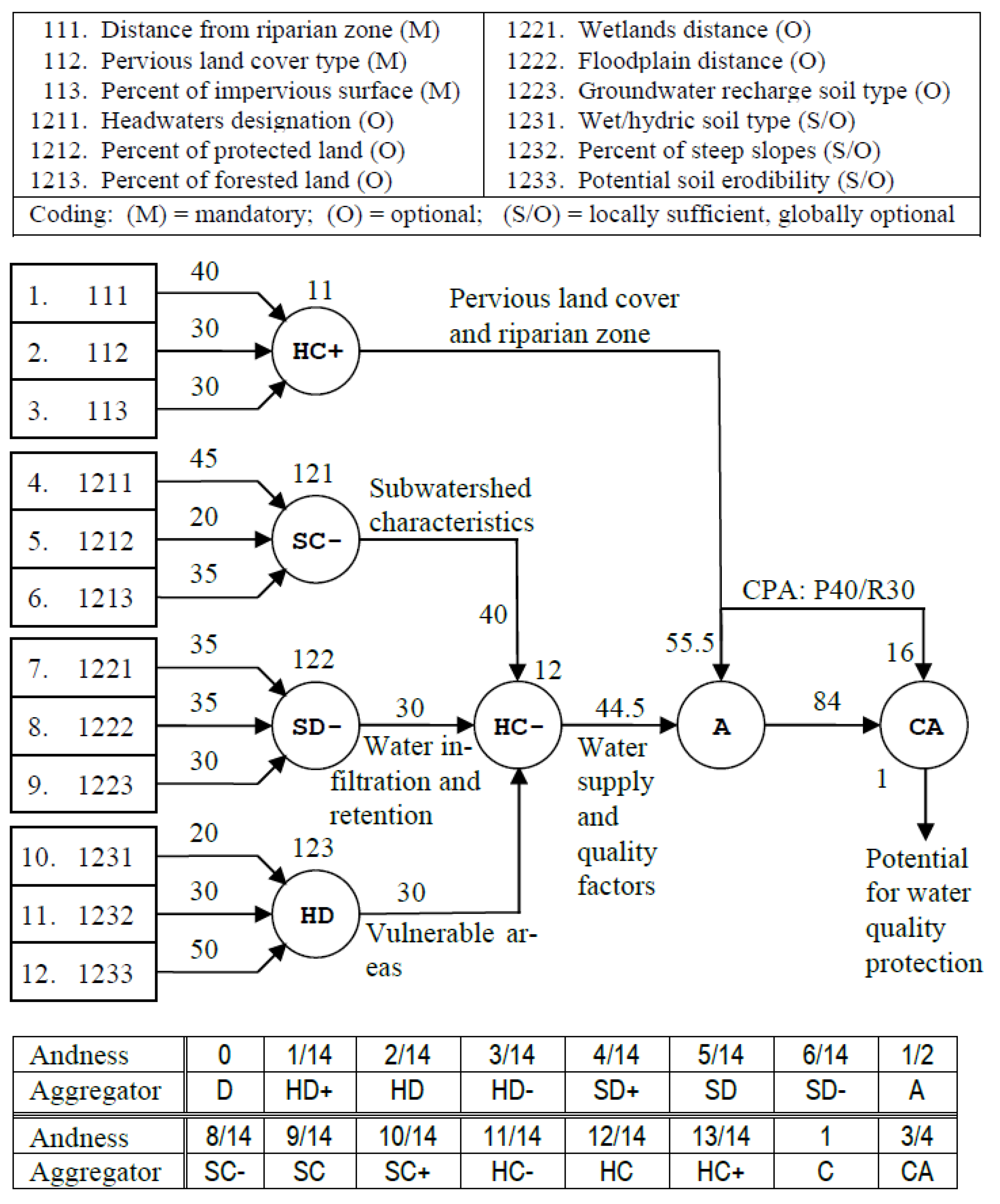
The decision-making explainability problems are related to specific LSP criterion. To illustrate such problems, we will use the criterion for the Upper Neuse Clean Water Initiative in North Carolina [7,8]. The goal is to evaluate specific locations and areas based on their potential for water quality protection. The evaluation team identified 12 attributes that contribute to the potential for water quality protection resulting in the LSP criterion shown in Figure 1. The stakeholders want to protect undeveloped lands near stream corridors that have soils that can absorb/hold water so that it is possible to avoid erosion and sedimentation and promote groundwater recharge and flood protection.

The aggregation structure in Figure 1 is based on medium precision aggregators [1] with three levels (low, medium, high) of hard partial conjunction (HC−, HC, HC+) supporting the annihilator 0, hard partial disjunction (HD−, HD, HD+), supporting the annihilator 1, and soft conjunctive (SC−, SC, SC+) and disjunctive (SD−, SD, SD+) aggregators that do not support annihilators. These are uniform aggregators where the threshold andness is 75% (aggregators with andness or orness above 75% are hard, and aggregators with andness or orness below 75% are soft).

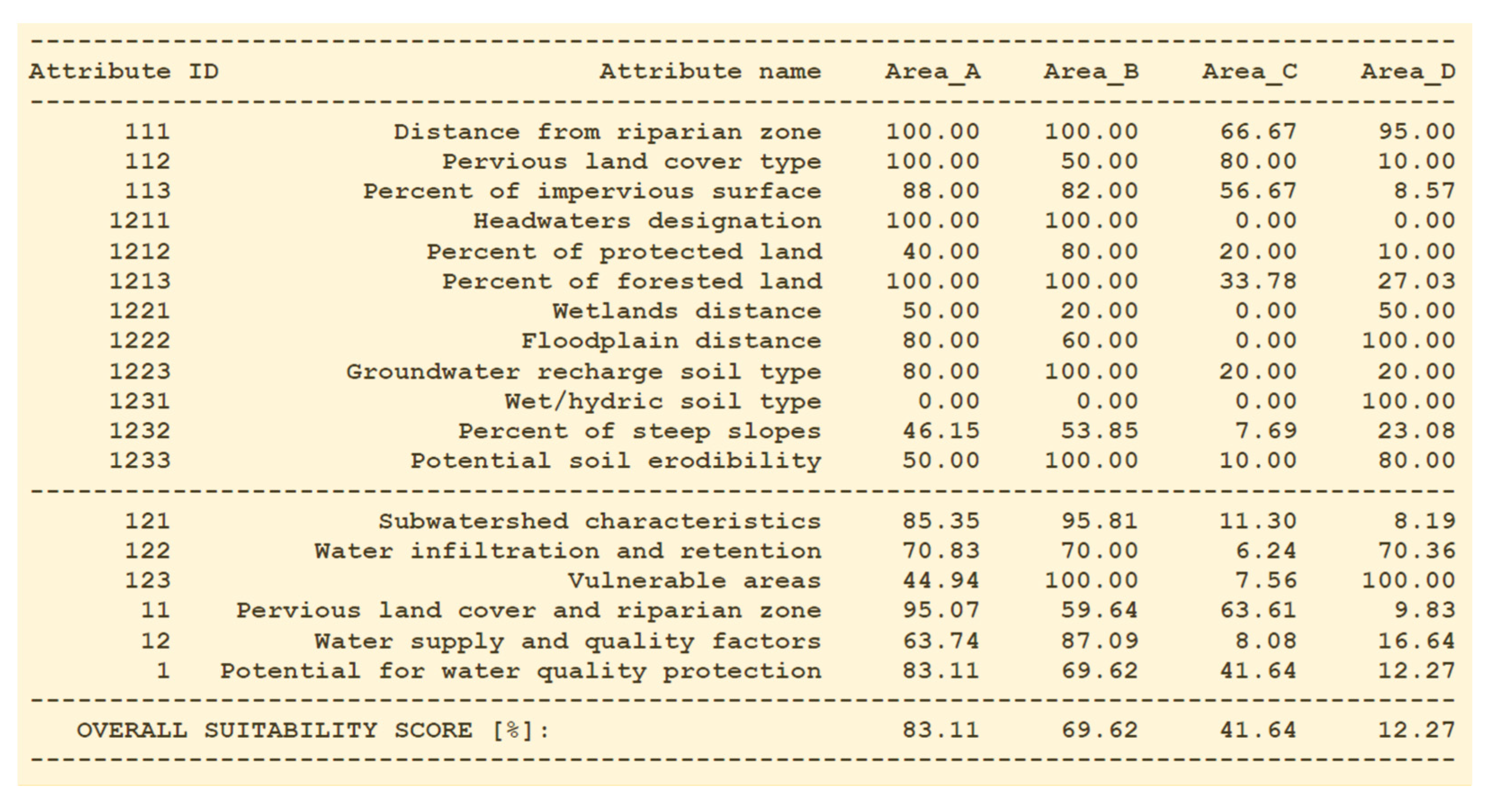
The nodes in the aggregation structure in Figure 1 are numbered according to the LSP aggregation tree structure where the root node (overall suitability) is the node number 1, and generally, the child nodes of node N are denoted N1, N2, N3, and so on (e.g., the node N = 11 has child nodes 111, 112, 113). In Figure 1, for simplicity, we also numbered inputs 1, 2, …, 12, so that the input attributes are $a_1,a_2,\dots a_n, a_i\in ℝ, i=1,\dots ,n; n=12,$ and their attribute suitability scores that belong to $I=\left[0,1\right]$ are $x_1,x_2,\dots x_n, x_i\in I, i=1,\dots ,n$. The overall suitability is a graded logic function $L:I^n\to I$ of attribute suitability scores: $X=L(x_1,x_2,\dots x_n)$. The details of attribute criteria can be found in [8], and the results of evaluation and comparison of four competitive areas (denoted A, B, C, D), based on the criterion shown in Figure 1, are presented in Figure 2.

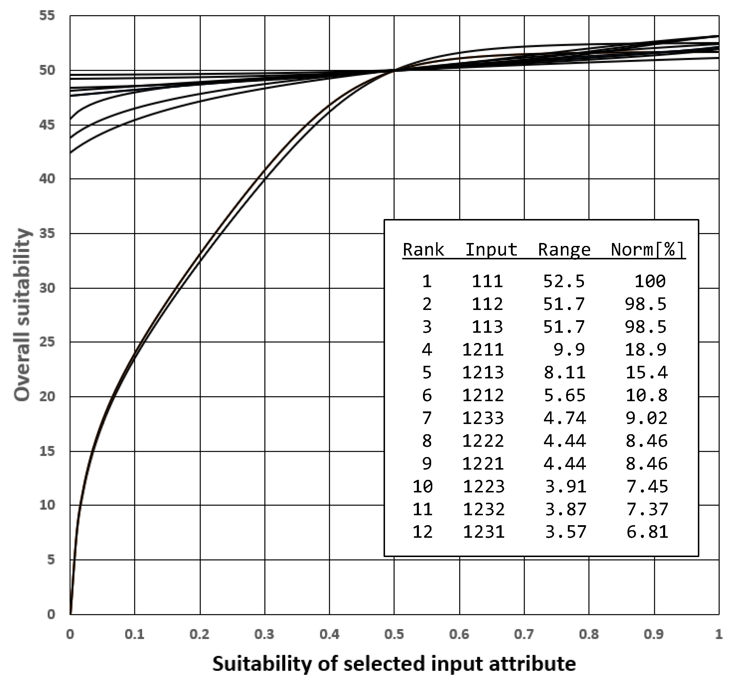
The point of departure in explaining the properties of the logic aggregation structure is the survey of sensitivity curves $X_i\left(x_i\right)=L(x_1,\dots ,x_i,\dots x_n)$, $x_k=c, k\ne i$, where c denotes a selected constant; typically, $c=0.5$. The sensitivity curves show the impact of a single input, assuming that all other inputs are constant. Figure 3 shows the sensitivity curves for the aggregation structure used in Figure 1, in the case of $c=0.5$.

The relative impact of individual inputs can be estimated using the values of the output suitability range $r_i[\%]=100 \left[X_i\left(1\right)-X_i\left(0\right)\right], i=1,\dots ,n$, and their maximum-normalized values $R_i[\%]=100 r_i/\max (r_1,\dots ,r_n), i=1,\dots ,n$. These indicators show the change of overall suitability caused by the individual change of selected input attribute suitability in the whole range from 0 to 1. Therefore, $R_i[\%]$ is one of indicators of the overall impact (or the overall importance) of the given suitability attribute. The corresponding ranking of attributes from the most significant to the least significant should be intuitively acceptable, explainable, and approved by the stakeholder. That is achieved in the ranking shown in Figure 3 where the first three attributes (111, 112, 113) are mandatory, and all others are optional with different levels of impact. That is consistent with stakeholder requirements specified before the development of the criterion shown in Figure 1. The normalized values $R_1,\dots ,R_n$ depend on the value of constant c, but their values and ranking are rather stable. In Figure 3 we use $c=0.5$. If $c=0.75$, the ranking of the first six most significant inputs remains unchanged. Minor permutations occur in the bottom six less significant inputs.

The explainability of LSP evaluation project results is a process consisting of the following three main components:

• Explainability of the LSP criterion

  1.1.

  Explainability of attributes

  1.2.

  Explainability of elementary attribute criteria

  1.3.

  Explainability of suitability aggregation structure

• Explainability of evaluation of individual alternatives

  2.1.

  Analysis of concordance values

  2.2.

  Classification of contributors

• Explainability of comparison of competitive alternatives

  3.1.

  Analysis of explainability indicators of individual alternatives

  3.2.

  Analysis of differential effects

The explainability of LSP criterion is defined as a general justification of the validity of criterion (i.e., the consistency between requirements/expectations and the resulting properties of criterion) without considering the available alternatives. In other words, this analysis reflects independent properties of a proposed criterion function. Most actions in the development of an LSP criterion are self-explanatory. The development of a suitability attribute tree is directly based of stakeholder goals, interests, and requirements. The selected suitability attributes should be necessary, sufficient, and nonredundant. Explainability of this step should list reasons why all attributes are necessary and sufficient. In our example, the tree is indirectly visible in Figure 1. The attribute criteria (shown in [8]) come with descriptions that for each attribute criterion provide the explanation of reasons for a selected evaluation method. Regarding the suitability aggregation structure (Figure 1), the only contribution to explainability consists of the sensitivity analysis for constant inputs and for ranking of the overall impact/importance of suitability attributes. All other contributions to explainability are based on specific values of inputs that characterize competitive alternatives.

3. Concordance Values and Explainability of Evaluation Results

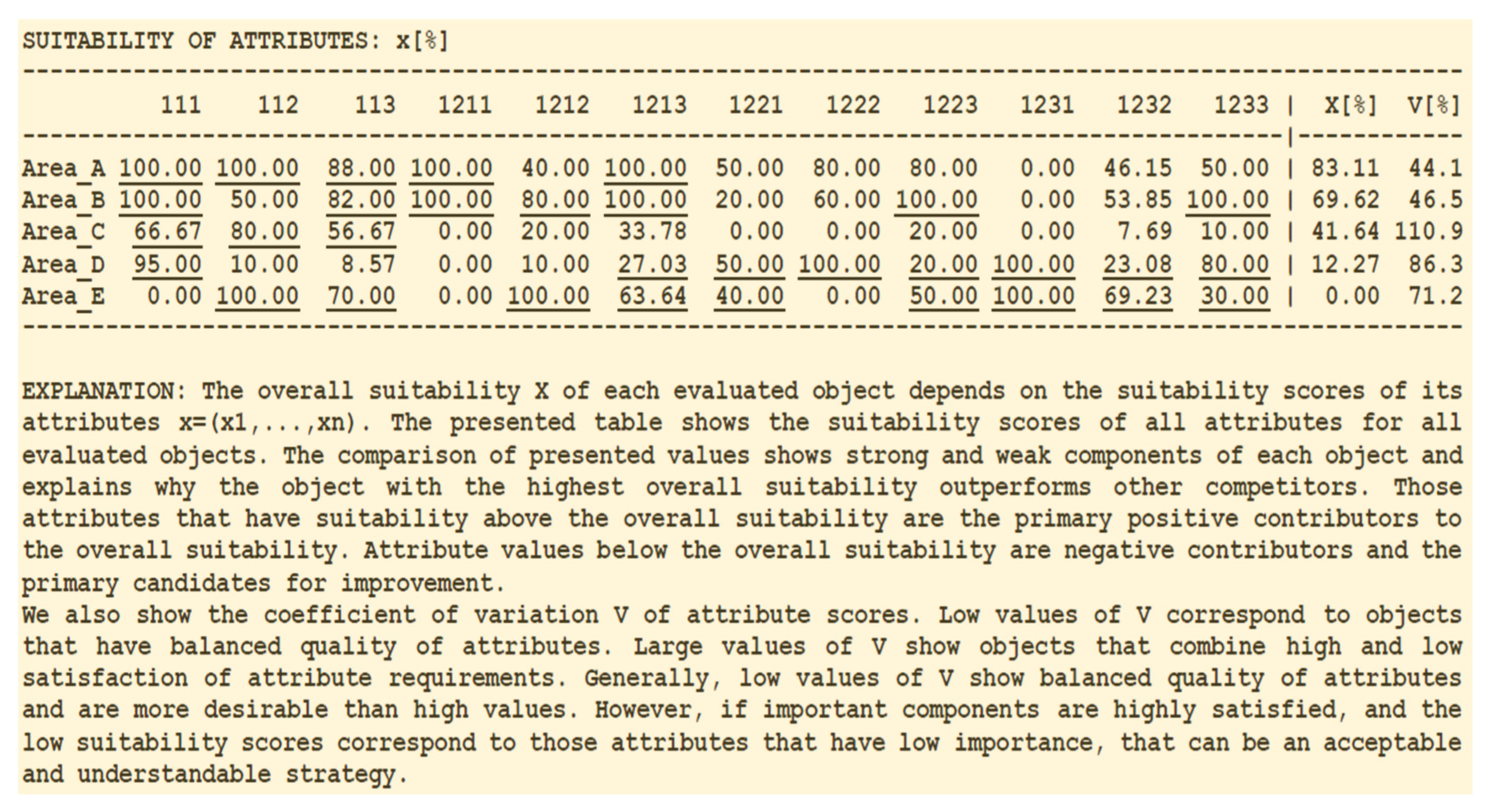
In the case of evaluation of a specific object/alternative, each suitability attribute can provide different contributions to the overall suitability $X$. In the most frequent case of idempotent aggregation structures, we differentiate two groups of input attributes: high contributors and low contributors. High contributors are inputs where $x_i>X$; such attribute values are “above the average” and contribute to the increase of the overall suitability. Similarly, low contributors are inputs where $x_i<X$; such attribute values are “below the average” and contribute to the decrease of the overall suitability. Figure 4 shows the comparison of five areas and all high contributor values are underlined. The overall suitability $X$ shows the resulting ranking of analyzed areas: A > B > C > D > E.

For each attribute, there is obviously a balance point $x_i^{*}$ where the i^th input is in perfect balance with remaining inputs. This value is called the concordance value and it is crucial for explainability analysis. For all input attributes, the concordance values can be obtained by solving the following equations:

$$x_i^{*}=L\left(x_1,\dots ,x_{i-1},x_i^{*},x_{i+1},\dots ,x_n\right),\hspace{0.17em}\hspace{0.17em}i=1,\dots ,n$$

According to the fixed-point iteration concept [11], these equations can be solved, for each of $n$ attributes, using the following simple convergent numerical procedure:

$$\begin{array}{l}\mathsf{\epsilon }=0.0000001;\hspace{1em}\hspace{1em}// \mathrm{or} \mathrm{any} \mathrm{other} \mathrm{small} \mathrm{value} \mathrm{that} \mathrm{defines} \mathrm{the} \mathrm{precision} \mathrm{of} x_i^{*}\\ x_i^{*}=0.5;\hspace{1em}\hspace{1em}\hspace{1em}\hspace{1em}// \mathrm{or} \mathrm{any} \mathrm{other} \mathrm{initial} \mathrm{value} \mathrm{inside} \mathrm{the} \mathrm{interval} [0,1]\\ \mathbf{do}\\ \hspace{1em}\hspace{1em}{x}_i^{*}=L(x_1,\dots , x_{i-1}, x_i^{*}, x_{i+1}, \dots , x_n);\\ \mathbf{while} \left(\right|x_i^{*}-L(x_1,\dots , x_{i-1}, x_i^{*}, x_{i+1}, \dots , x_n\left)\right| > \mathsf{\epsilon })\end{array}$$

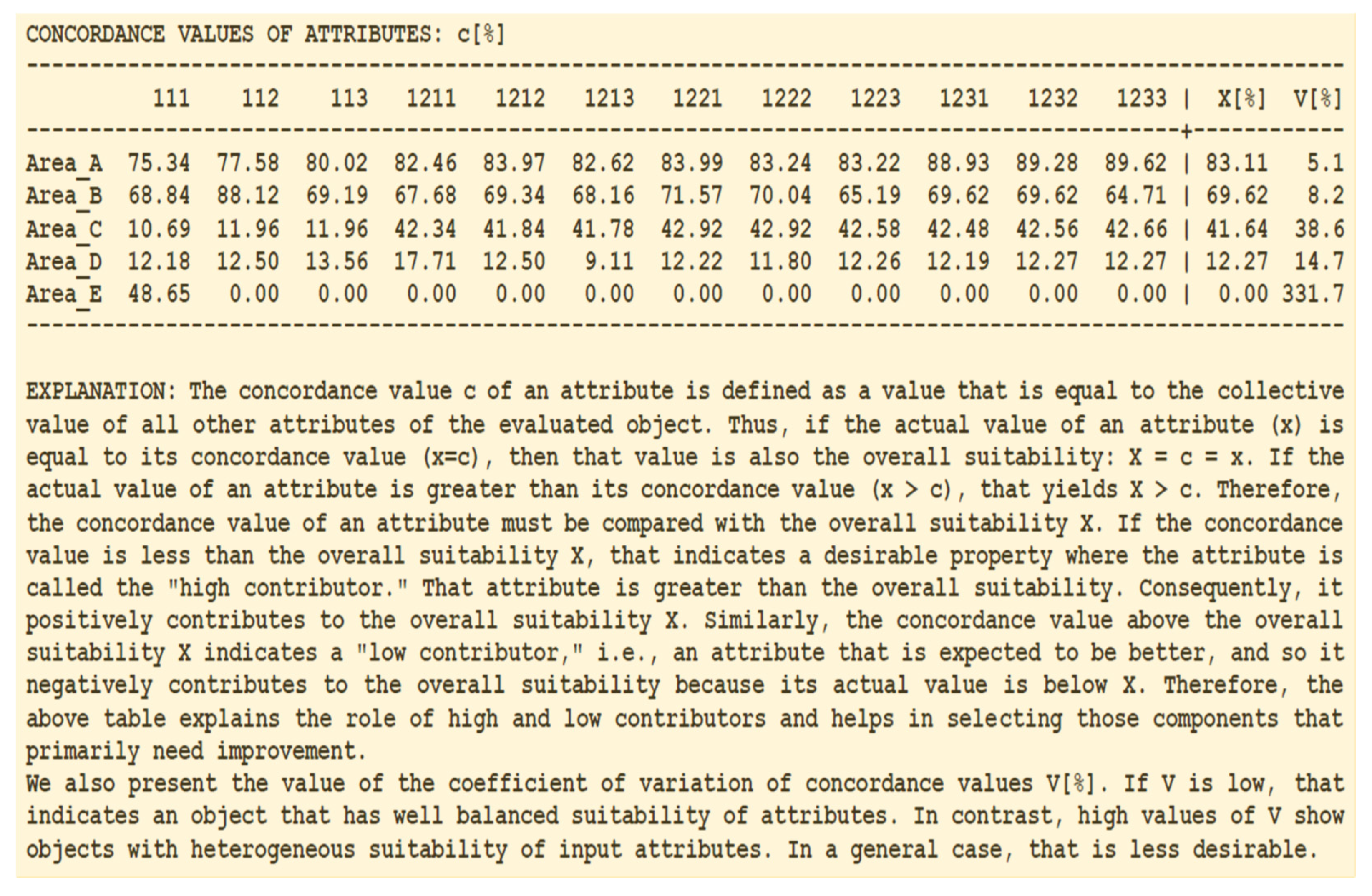
The concordance values of all attributes for five competitive conservation areas, generated by LSP.XRG, are shown in Figure 5. Note that the values of all attributes $x_k, k\ne i$, are not constants; they are the real values that correspond to the selected competitive area. The concordance value $x_i^{*}$ shows the collective quality of all inputs different from i. If other inputs are high, then the concordance value of the ith input will also be high, reflecting the general demand for balanced, high satisfaction of inputs. Thus, the concordance values $x_i^{*}>X$ indicate low contributors, while $x_i^{*}\le X$ characterizes high contributors as shown in Figure 5 (in all LSP.XRG results the concordance values are denoted c). According to Figure 4 and Figure 5, the Area_E does not satisfy the mandatory requirement 111 (it is too far from the riparian zone) and therefore it is considered unsuitable and rejected by our evaluation criterion. So, the area_E will not be included in subsequent explanations.

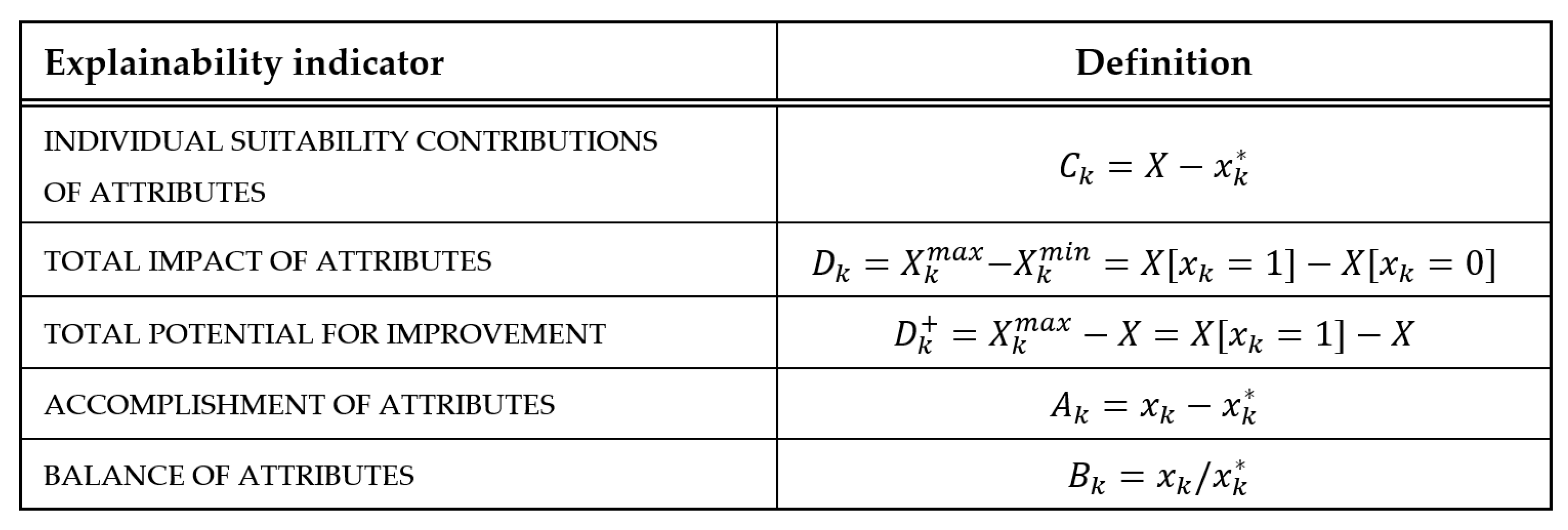
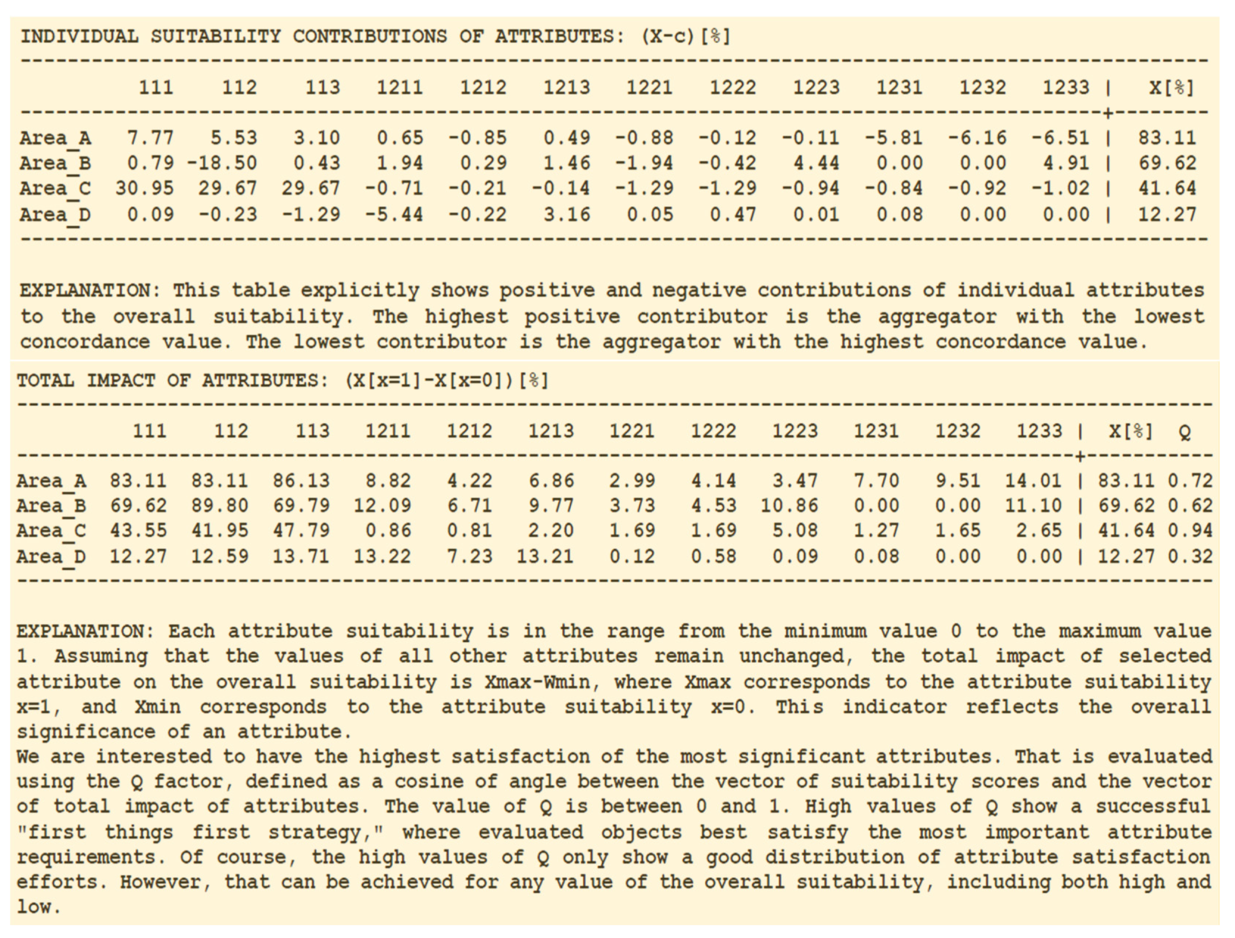
The concordance values are suitable for explaining convenient and inconvenient properties of the specific evaluated area. Indicators that are proposed for explanation are defined in Figure 6, and then applied and described in detail in Figure 7. The first question that most stakeholders ask is how individual attributes contribute to the overall suitability X. Since all values $x_1,\dots ,x_n$ contribute to the value of X, the most significant individual contributions come from inputs that have the lowest concordance values. Positive contributions shown in the individual contribution table in Figure 6 correspond to high contributors and negative to low contributors. For example, the primary reason for the highest suitability of the Area_A (with individual contribution of 7.77%) comes from the proximity to riparian zone followed by the convenient pervious land cover type (5.53%) and low percent of impervious surface (3.1%). The individual contributions depend on the structure of the LSP criterion. For example, according to Figure 4, the Area_A attributes 111, 112, 1211, 1213 have the highest suitability, but their individual contributions are in the range from 0.49% to 7.7%. The negative contributions of Area_A are in vulnerable areas attributes 1231, 1232, 1233 (each of them close to 6%).

The overall impact of individual attributes is an indicator similar to the overall importance of attributes derived from sensitivity curves (defined as the range in Figure 3). There is a difference: now we analyze the sensitivity of individual attributes based on real values of attributes of each individual alternative (areas A, B, C, D). That offers the possibility for ranking of attributes of individual alternatives according to their impact and (in cases where that is possible) to focus attention on the high impact attributes. However, the high impact is not the same concept as the high potential for improvement.

The potential for improvement is defined in Figure 7 as a real possibility to improve the overall suitability of an alternative. For example, the highest impact attributes of Area_A are already satisfied, and the highest potential for improvement comes from attributes that are insufficiently satisfied. So, the potential for improvement is an indicator that shows (in situations where that is possible) the most impactful attributes that should have the priority in the process of improvement. Their maximum values show the highest potential for improvement of each alternative. Of course, that assumes the possibility of adjustment; unfortunately, physical characteristics of locations and areas cannot be changed.

If an attribute has the value that is significantly above the concordance value, that indicates a high accomplishment, because the quality of that attribute is significantly above the collective quality of other attributes. Exceptionally high accomplishments in a few attributes (e.g., 111, 1222, and 1231 in the case of Area_D) are insufficient to provide high overall suitability and are also an indicator of low suitability of remaining attributes, yielding low ranking of areas D and E (Figure 4). In the case of Area_E, a single negative accomplishment in a mandatory attribute 111 is sufficient to reject that alternative.

The concordance values offer an opportunity to analyze the balance of attributes. If all attributes are close to their concordance values, that denotes a highly balanced alternative where all attributes have a similar quality. The coefficient of variation (V[%]) of the ratios of actual and concordance values of attributes shows the degree of imbalance and in Figure 6 the lower quality areas C and D are also significantly imbalanced. Of course, the low imbalance does not mean high suitability; an alternative can have a highly balanced low quality. However, high imbalance generally shows alternatives that need to be improved. Note that the imbalance of attributes in Figure 7 has the same ranking as the coefficient of variation of the concordance values in Figure 5; these concepts are similar.

4. Explainability of the Comparison of Alternatives

Explainability of evaluation results contributes to understanding the results of ranking of individual alternatives. However, stakeholders are regularly interested in explaining the specific reasons why an alternative is superior/inferior compared to another alternative. Consequently, the comparison of alternatives needs explanations focused on discriminative properties of LSP criteria.

The superiority of the leading alternative in an evaluation project is a collective effect of all inputs and it cannot be attributed to a single attribute. However, an estimate of individual effects can be based on the direct comparison of the suitability degrees of individual attributes. Suppose that the Area_A has the attribute suitability degrees $a_1,\dots ,a_n$, and the Area_B has the attribute suitability degrees $b_1,\dots ,b_n$. Then, according to Figure 4, we have $X_A=L(a_1,\dots ,a_n)=83.1\%$ and $X_B=L(b_1,\dots ,b_n)=69.6\%$. An estimate of the individual effect of attribute $a_i, i\in \left\{1,\dots ,n\right\}$, compared to the same attribute in the Area_B, can be obtained using the discriminators of attributes

$$R_i\left(A,B\right)=X_A-L(a_1,\dots ,a_{i-1},b_i,a_{i+1},\dots ,a_n), i=1,\dots ,n$$

Similarly,

$$R_i\left(B,A\right)=X_B-L(b_1,\dots ,b_{i-1},a_i,b_{i+1},\dots ,b_n), i=1,\dots ,n$$

The discriminator $R_i\left(A,B\right)$ shows the individual contribution of selected attribute to the ranking A > B. If $R_i\left(B,A\right)>0$ then the selected attribute positively contributes to the ranking A > B; similarly, if $R_i\left(B,A\right)<0$, then the selected attribute negatively contributes to the ranking A > B. If $b_i=a_i$, then there is no contribution of the selected attribute. We use n discriminators for all n attributes to explain the individual attribute contributions to the ranking of two objects/alternatives. This insight can significantly contribute to explainability reports.

If $R_i\left(A,B\right)>0$, then $a_i$ positively contributes to the ranking A > B, and to condition $R_i\left(A,B\right)\times R_i\left(B,A\right)\le 0$ (i.e., their signs are different). Since the discriminators $R_i\left(A,B\right), i=1,\dots ,n$ show the superiority of attributes of the Area_A with respect to the attributes of the Area_B, and $R_i\left(B,A\right)$ shows the superiority of attributes of the Area_B with respect to the attributes of the Area_A, it follows that these are two different views of the same relationship between two alternatives. To consider both views, we can average them and compute the mean superiority of the Area_A with respect to the Area_B for specific attributes as follows:

$$M_i\left(A,B\right)=\left[R_i\left(A,B\right)-R_i\left(B,A\right)\right]/2, i=1,\dots ,n$$

An overall indicator of superiority can be now defined as a “mean overall superiority”

$$M\left(A,B\right)=\frac{1}{n}{{\displaystyle \sum }}_{i=1}^n{M}_i\left(A,B\right)$$

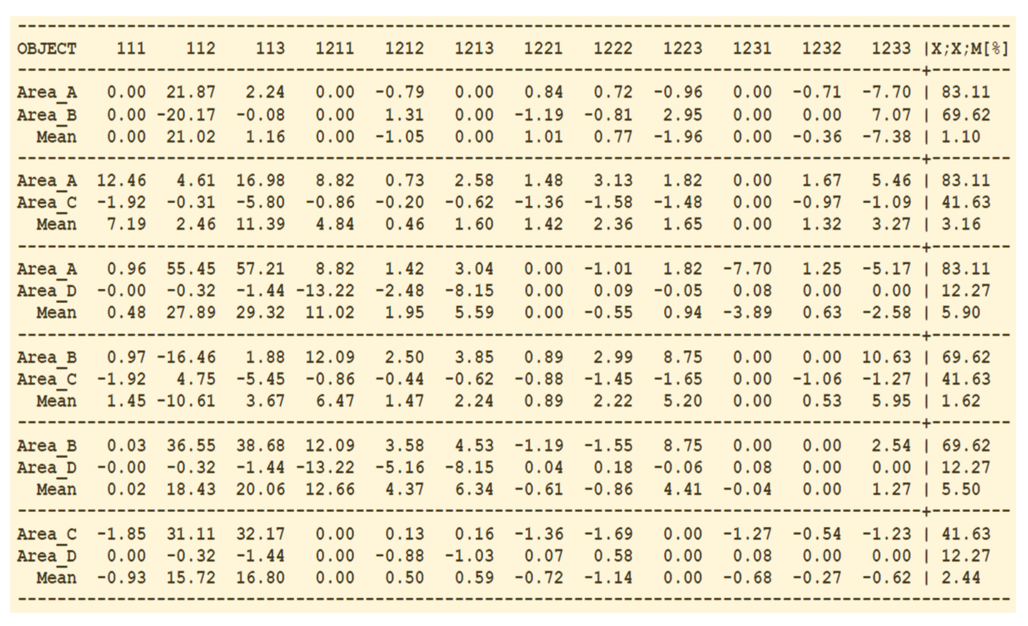
The pairwise comparison of areas A, B, C, D is shown in Figure 8. The first three rows contain the comparison of areas A and B. The first row contains discriminators $R_i\left(A,B\right)$, and the second row contains discriminators $R_i\left(B,A\right)$. The mean superiority $M_i\left(A,B\right)$ is computed in the third row. The rightmost column shows the overall suitability scores of competitive objects ($X_A$ and $X_B$), followed by the mean overall superiority of the first object, $M\left(A,B\right).$ It should be noted that the individual attribute superiority indicators $M_i\left(A,B\right), i=1,\dots ,n$ are useful for comparison of objects, and discovering critical issues, but they do not take into account the difference in importance between attributes. So, $M\left(A,B\right)$ shows unweighted superiority which is different from the difference in the overall suitability. Thus, we can investigate the values of the indicator $r=(X_A-X_B)/M\left(A,B\right)$. In our examples that value is rather stable (from 10.42 to 17.25), but not constant. This result shows that the overall indicator of superiority $M\left(A,B\right)$ is a useful auxiliary indicator for estimation of relationships between two competitive objects. The main contribution of discriminators to explainability is that they clarify the aggregator-based origins of dominance of one object with respect to another object.

From the standpoint of explainability of the comparison of objects, the individual indicators $M_i\left(A,B\right)$ explicitly show the predominant strengths (as high positive values) and predominant weaknesses (as low negative values) of the specific object. For example, in Figure 8, the main advantage of the Area_A compared to the Area_B is the attribute 112 (pervious land cover) and the main disadvantage is attribute 1233 (potential soil erodibility). Such relationships are useful for summarized verbal explanations of a proposed decision that the protection of Area_A should have priority with respect to the protection of Area_B).

In cases where that is possible, the explicit visibility of disadvantages and weaknesses is useful for explaining what properties should be improved, and in what order. Of course, some evaluated objects (e.g. computer systems, cars, airplanes, etc.) have the possibility to modify suitability attributes in order to increase their overall suitability. In such cases, the explainability indicators such as the potential for improvement, the individual suitability contributions, and the individual superiority scores, provide the guidelines for selecting the most effective corrective actions. In the case of locations and areas that are suitable for the water quality protection, the suitability attributes are physical properties that cannot be modified by decision-makers. In such cases the resulting potential for water quality protection cannot be changed, but the ranking of areas and explainability indicators are indispensable to make correct and trustworthy decisions about various protection and development activities.

5. Explainability Report as a Part of the Decision Documentation

Documentation of evaluation projects includes several main components. Each project starts with the specification of goals and interests of the stakeholder and the reasons for evaluating and selecting specific objects/alternatives. The next step is to develop the suitability attribute tree and elementary suitability attribute criteria that justifiably reflect the needs of the stakeholder. The suitability attributes are classified in basic groups of mandatory, optional, and sufficient inputs. These requirements are then implemented using appropriate logic aggregators in the suitability aggregation structure. This part of documentation is completed before the evaluation process. To justify the LSP criterion, it is useful to show sensitivity curves and to compute the ranking of importance of suitability attributes.

The evaluation process starts by documenting the available objects/alternatives. Then, the results of evaluation are presented as the suitability in each node of the aggregation structure, from input suitability degrees $x_1,\dots ,x_n$ to the overall suitability X. The ranking of alternatives is based on the decreasing values of the overall suitability scores. The highest suitability score indicates the alternative that is proposed for selection and implementation. In cases where alternatives have costs, the suitability and affordability are conjunctively aggregated to compute the overall value score [1] which is then used for selecting the best alternative.

In addition to the above traditional documentation, generated using LSP.NT [12], in this paper we introduced an additional explainability report that provides the explanation and justification of obtained results. That report is generated by the LSP Explainability Report Generator (LSP.XRG) tool. The results generated by LSP.XRG are exemplified in Figure 2, Figure 3, Figure 4, Figure 5, Figure 7 and Figure 8. The explainability report is based primarily on the following set of explainability indicators:

• Overall importance of suitability attributes (based on evaluation criterion)
• Concordance values of suitability attributes for each alternative
• Individual suitability contributions of attributes
• Total impact of individual suitability attributes for each alternative, and sensitivity analysis curves
• Total potential for improvement for each suitability attribute and for each competitive object/alternative
• Accomplishments of individual attributes for each alternative
• Balance of attribute values for each alternative
• Pairwise comparison of competitive objects/alternatives

In the case of evaluation of various locations/areas from the standpoint of their potential for water quality protection we provided the explainability indicators in Figure 4, Figure 5, Figure 7 and Figure 8. These indicators can be used in several ways. First, all tables with results can be automatically generated by LSP software support tools. Then, it is possible to compose a verbalized summary report based on explainability indicators. Finally, the information stored in explainability tables created by the LSP.XRG can be selectively inserted in executive summaries and used during stakeholder meetings and approval processes. The explainability results and explainability documentation significantly contribute to the confidence that stakeholders must have in evaluation results and proposed decisions.

6. Conclusions

Decisions are results of human mental activities, and consequently all decision methods should have a strong humancentric component. That includes the explainability of proposed decisions. Trustworthiness and explainability are currently important topics (and active research areas) particularly in cases where AI tools are used to automatically discover knowledge in large databases and propose decisions that affect human conditions and actions. In such cases, the trustworthiness of decisions becomes the critical issue.

In this paper we have shown that explainability and trustworthiness are equally important and useful also in the decision-making process that involves a permanent presence of humans as stakeholders, decision engineers, domain experts, and executives. This process includes the specification of alternatives, the development of evaluation criteria, the specification of requests to vendors or system developers, and the final evaluation of competitive alternatives, selection of the best alternative, and justifying the decision to approve its implementation.

The proposed explainability indicators and their use are developed in the context of the LSP decision method, where all explanatory presentations can be integrated in a specific explainability report. Our example of the Upper Neuse Clean Water Initiative in North Carolina was selected as a realistic decision project where explainability is important because of the large number of stakeholders, which include all interested in the protection of clean water supply in perpetuity. That includes municipalities, companies, various social organizations, and individual citizens. For all decisions in this situation, it is necessary to provide convincing evaluation results, as well as verbal and quantified explanations. In this paper we proposed a solution of that problem. The same methodology is equally applicable in practically all other decision projects based on the LSP method.

References

- Dujmović, J. Soft Computing Evaluation Logic; Wiley and IEEE Press: Hoboken, NJ, USA, 2018. [Google Scholar]
- Alonso-Moral, J.M.; Mencar, C.; Ishibuchi, H. Explainable and Trustworthy Artificial Intelligence. Comput. Intell. 2022, 17, 14–15. [Google Scholar]
- Deng, Y.; Weber, G.W. Fuzzy Systems toward Human-Explainable Artificial Intelligence and Their Applications. IEEE Trans. Fuzzy Syst. 2021, 29, 3577–3578. [Google Scholar]
- Wing, J.M. Trustworthy AI. Commun. ACM 2021, 64, 64–71. [Google Scholar] [CrossRef]
- De Tré, G.; Dujmović, J. Dealing with Data Veracity in Multiple Criteria Handling: An LSP-Based Sibling Approach. In Proceedings of the International Conference on Flexible Query Answering Systems, FQAS 2021, Bratislava, Slovakia, 16 September 2021. In Flexible Query Answering Systems; Larsen, H.L., Martin-Bautista, M.J., Vila, M.A., Andreasen, T., Christiansen, H., Eds.; Springer: Berlin/Heidelberg, Germany, 2021; pp. 82–96. [Google Scholar]
- Dujmović, J. Interpretability and Explainability of LSP Evaluation Criteria. In Proceedings of the 2020 IEEE World Congress on Computational Intelligence, Glasgow, UK, 19–24 July 2020. 978-1-7281-6932-3/20, Paper F-22042 (2020). [Google Scholar]
- Conservation Trust for North Carolina. 2020. Available online: https://ctnc.org/impressive-accomplishments-already/ (accessed on 19 March 2022).
- Dujmović, J.; Allen, W.L., III. Soft Computing Logic Decision Making in Strategic Conservation Planning for Water Quality Protection. Ecol. Inform. 2021, 61, 101167. [Google Scholar] [CrossRef]
- Messer, K.; Allen, W. The Science of Strategic Conservation Planning: Protecting More with Less; Cambridge University Press: Cambridge, UK, 2018. [Google Scholar]
- Benedict, M.; McMahon, E. Green Infrastructure: Linking Landscapes and Communities; Island Press: Washington, DC, USA, 2006. [Google Scholar]
- Polyanin, A.D.; Manzhirov, A.V. Handbook of Mathematics for Engineers and Scientists; Chapman & Hall/CRC: London, UK, 2007. [Google Scholar]
- SEAS Co. LSP.NT—LSP Method for Evaluation over the Internet. LSP.NT V1.2 User Manual. Available online: http://www.seas.com/LSPNT/login.php (accessed on 17 November 2022).
Figure 1.
Twelve suitability attributes, the suitability aggregation structure, and the andness of medium precision hard (H) and soft (S), conjunctive (C) and disjunctive (D) aggregators used in the LSP criterion for evaluation of the potential for water quality protection.
Figure 2.
Results of evaluation of four areas (A, B, C, and D): suitability [%] for all inputs and for all subsystems of the aggregation structure shown in Figure 1.
Figure 3.
Sensitivity curves and ranking of attributes using the normalized range of impact.
Figure 4.
Suitability of attributes and the global suitability of five competitive areas (the underlined values indicate the high contributors).
Figure 5.
Concordance values, their coefficient of variation (V[%]) and the global suitability (X[%]) of five competitive areas (the concordance values below the overall suitability show the high contributors). This is one of outputs generated by LSP.XRG.
Figure 6.
Basic explainability indicators.
Figure 7.
Indicators used for explaining the evaluation results (output generated by LSP.XRG).
Figure 8.
Pairwise comparison of competitive areas A, B, C, and D.
Publisher’s Note: MDPI stays neutral with regard to jurisdictional claims in published maps and institutional affiliations. |
© 2022 by the authors. Licensee MDPI, Basel, Switzerland. This article is an open access article distributed under the terms and conditions of the Creative Commons Attribution (CC BY) license (https://creativecommons.org/licenses/by/4.0/).
Share and Cite
MDPI and ACS Style
Dujmović, J.; Allen, W.L., III. Explainable Decision-Making for Water Quality Protection. Information 2022, 13, 551. https://doi.org/10.3390/info13120551
AMA Style
Dujmović J, Allen WL III. Explainable Decision-Making for Water Quality Protection. Information. 2022; 13(12):551. https://doi.org/10.3390/info13120551
Chicago/Turabian StyleDujmović, Jozo, and William L. Allen, III. 2022. "Explainable Decision-Making for Water Quality Protection" Information 13, no. 12: 551. https://doi.org/10.3390/info13120551
Note that from the first issue of 2016, this journal uses article numbers instead of page numbers. See further details here.