Evaluating the Performance of Structure from Motion Pipelines

Abstract

Structure from Motion (SfM) is a pipeline that allows three-dimensional reconstruction starting from a collection of images. A typical SfM pipeline comprises different processing steps each of which tackles a different problem in the reconstruction pipeline. Each step can exploit different algorithms to solve the problem at hand and thus many different SfM pipelines can be built. How to choose the SfM pipeline best suited for a given task is an important question. In this paper we report a comparison of different state-of-the-art SfM pipelines in terms of their ability to reconstruct different scenes. We also propose an evaluation procedure that stresses the SfM pipelines using real dataset acquired with high-end devices as well as realistic synthetic dataset. To this end, we created a plug-in module for the Blender software to support the creation of synthetic datasets and the evaluation of the SfM pipeline. The use of synthetic data allows us to easily have arbitrarily large and diverse datasets with, in theory, infinitely precise ground truth. Our evaluation procedure considers both the reconstruction errors as well as the estimation errors of the camera poses used in the reconstruction.

1. Introduction

Three-dimensional reconstruction is the process that allows to capture the geometry and appearance of an object or an entire scene. In the last years, interest has developed around the use of 3D reconstruction for reality capture, gaming, virtual and augmented reality. These techniques have been used to realize video game assets [1,2], virtual tours [3] as well as mobile 3D reconstruction apps [4,5,6]. Some other areas in which 3D reconstruction can be used are CAD (Computer Aided Design) software [7], computer graphics and animation [8,9], medical imaging [10], virtual and augmented reality [11], cultural heritage [12], etc…

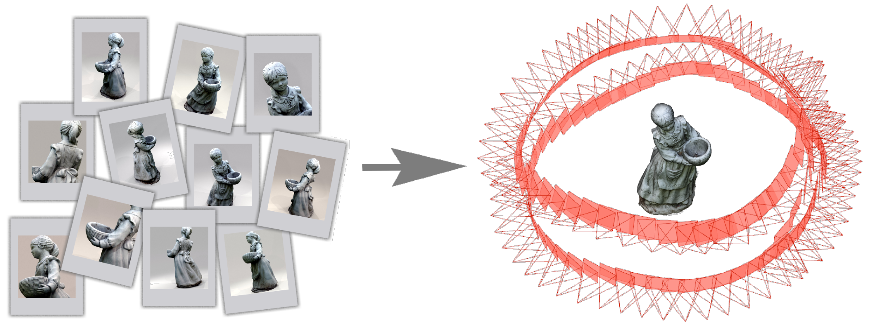
Over the years, a variety of techniques and algorithms for 3D reconstruction has been developed to meet different needs in various fields of application ranging from active methods that require the use of special equipment to capture geometry information (i.e., laser scanners, structured lights, microwaves, ultrasound, etc...) to passive methods that are based on optical imaging techniques only. The latter techniques do not require special devices or equipment and thus are easily applicable in different contexts. Among the passive techniques for 3D reconstruction there is the Structure from Motion (SfM) pipeline [13,14,15,16,17]. As shown in Figure 1, given a set of images acquired from different observation points, it recovers the pose of the camera for each input image and a three-dimensional reconstruction of the scene in form of a sparse point cloud. After this first sparse reconstruction, it is possible to run a dense reconstruction phase using Multi-View Stereo (MVS) [18].

As it can be seen from Figure 2, a typical SfM pipeline comprises different processing steps each of which tackles a different problem in the reconstruction pipeline. Each step can exploit different algorithms to solve the problem at hand and thus many different SfM pipelines can be built. There are many SfM pipelines available in the literature. How to choose the best among them?

In this paper, we compare different state-of-the-art SfM pipelines in terms of their ability to reconstruct different scenes. The comparison is carried out by evaluating the reconstruction error of each pipeline on an evaluation dataset. The dataset is composed of real objects whose ground truth has been acquired with high-end devices. Having real scenes as reference models is not trivial, thus we have developed a plug-in for a rendering software to create an evaluation dataset starting from synthetic 3D scenes. This allows us to rapidly and efficiently extend the existing datasets and stress the pipelines under various conditions.

The rest of the paper is organized as follows. In Section 2, we describe the incremental SfM pipeline building blocks and compare their implementations. In Section 3, we describe how we evaluated the different pipelines. In Section 4 we present a plug-in that allows to generate synthetic datasets, evaluate the SfM and MVS reconstructions. In Section 5 we present and comment the evaluation results. Section 6 concludes the paper. In Appendix A we provide some guidelines about how to best capture images to be used in a reconstruction pipeline.

2. Review of Structure from Motion

The SfM pipeline allows the reconstruction of three-dimensional structures starting from a series of images acquired from different observation points. The complete flow of incremental SfM pipeline operations is shown in Figure 2. In particular, incremental SfM is a sequential pipeline that consists of a first phase of correspondences search between images and a second phase of iterative incremental reconstruction. The correspondence search phase is composed of three sequential steps: Feature Extraction, Feature Matching and Geometric Verification. This phase takes as input the image set and generates as output the so called Scene Graph (or View Graph) that represents relations between geometrically verified images. The iterative reconstruction phase is composed of an initialization step followed by three reconstruction steps: Image Registration, Triangulation and Bundle Adjustment. Using the scene graph, it generates an estimation of the camera pose for each image and a 3D reconstruction as a sparse point cloud.

2.1. SfM Building Blocks

In this section we describe the building blocks of a typical incremental SfM pipeline illustrating the problem that each of them addresses and the possible solutions exploited.

Feature Extraction: For each image given in input to the pipeline, a collection of local features is created to describe the points of interest of the image (key points). For feature extraction different solutions can be used, the choice of the algorithm influences the robustness of the features and the efficiency of the matching phase. Once key points and their description is obtained, correspondences of these points in different images can be searched by the next step.

Feature Matching: The key points and features obtained through Feature Extraction are used to determine which images portray common parts of the scene and are therefore at least partially overlapping. If two points in different images have the same description, then those points can be considered as being the same in the scene respect to the appearance; if two images have a set of points in common, then it is possible to state that they portray a common part of the scene. Different strategies can be used to efficiently compute matches between images; solutions adopted by SfM implementations are reported in

Table 1. Incremental SfM pipelines algorithm comparison.

	Feature Extraction	Feature Matching	Geometric Verification	Image Registration	Triangulation	Bundle Adjustment	Robust Estimation
COLMAP	SIFT [31]	Exaustive	4 Point for Homography [20]	P3P [32]	sampling-based DLT [14]	Multicore BA [27]	RANSAC [19]
		Sequential	5 Point Relative Pose [33]	EPnP [34]		Ceres Solver [35]	PROSAC [36]
		Vocabulary Tree [37]	7 Point for F-matrix [20]				LO-RANSAC [38]
		Spatial [14]	8 Point for F-matrix [20]
		Transitive [14]
OpenMVG	SIFT [31]	Brute force	affine transformation	6 Point DLT [20]	linear (DLT) [20]	Ceres Solver [35]	Max-Consensus
	AKAZE [39]	ANN [40]	4 Point for Homography [20]	P3P [32]			RANSAC [19]
		Cascade Hashing [41]	8 Point for F-matrix [20]	EPnP [34]			LMed [42]
			7 Point for F-matrix [20]				AC-Ransac [43]
			5 Point Relative Pose [33]
Theia	SIFT [31]	Brute force	4 Point for Homography [20]	P3P [32]	linear (DLT) [20]	Ceres Solver [35]	RANSAC [19]
		Cascade Hashing [41]	5 Point Relative Pose [33]	PNP (DLS) [44]	2-view [45]		PROSAC [36]
			8 Point for F-matrix [20]	P4P [46]	Midpoint [47]		Arrsac [48]
				P5P [49]	N-view [20]		Evsac [50]
							LMed [42]
VisualSFM	SIFT [31]	Exaustive	n/a	n/a	n/a	Multicore BA [27]	RANSAC [19]
		Sequential
		Preemptive [16]
Bundler	SIFT [31]	ANN [51]	8 Point for F-matrix [20]	DLT based [20]	N-view [20]	SBA [52]	RANSAC [19]
						Ceres Solver [35]
MVE	SIFT [31] + SURF [53]	Low-res + exaustive [29]	8 Point for F-matrix [20]	P3P [32]	linear (DLT) [20]	own LM BA	RANSAC [19]
		Cascade Hashing

. The output of this phase is a set of images overlapping at least in pairs and the set of correspondences between features.

Geometric Verification: This phase of analysis is necessary because the previous matching phase only verifies that pairs of images apparently have points in common; it is not guaranteed that found matches are real correspondences of 3D points in the scene, outliers could be included. It is necessary to find a geometric transformation that correctly maps a sufficient number of points in common between two images. If this happens, the two images are considered geometrically verified, thus meaning that the points are also corresponding in the geometry of the scene. Depending on the spatial configuration with which the images were acquired, different methods can be used to describe their geometric relationship. An homography can be used to describe the transformation between two images of a camera that acquires a planar scene. Instead, the epipolar geometry allows to describe the movement of a camera through the essential matrix E if the intrinsic calibration parameters of the camera are known; alternatively, if the parameters are unknown, it is possible to use the uncalibrated fundamental matrix F. Algorithms used for geometric verification are reported in Table 1. Since the correspondences obtained from the matching phase are often contaminated by outliers, it is necessary to use robust estimation techniques such as RANSAC (RANdom SAmple Consensus) [19] during the geometry verification process [20,21]. Instead of RANSAC, some of its optimizations can be used to reduce execution times. Refer to Table 1 for a list of possible robust estimation methods. The output of this phase of the pipeline is the so-called Scene Graph, a graph whose nodes represent images and edges join the pairs of images that are considered geometrically verified.

Reconstruction Initialization: The initialization of the incremental reconstruction is an important phase because a bad initialization leads to a bad reconstruction of the three-dimensional model. To obtain a good reconstruction it is preferable to start from a dense region of the scene graph so that the redundancy of the correspondences provides a solid base for the reconstruction. In case the reconstruction starts from an area with few images, the Bundle Adjustment process does not have sufficient information to refine the position of the reconstructed camera poses and points; this leads to an accumulation of errors and a bad final result. For the initialization of the reconstruction a pair of geometrically verified images is chosen in a dense area of the scene graph. If more than one pair of images can be used as a starting point, the one with the most geometrically verified matching points is chosen. The points in common to the two images are used as the first points of the reconstructed cloud; they are also used to establish the pose of the first two cameras. Subsequently the Image Registration, Triangulation and Bundle Adjustment steps add iteratively new points to the reconstruction considering a new image at a time.

Image Registration: Image registration is the first step of the incremental reconstruction. In this phase a new image is added to the reconstruction and is thus identified as registered image. For the newly registered image the pose of the camera (position and rotation) that has acquired it must be calculated; this can be achieved using the correspondence with the known 3D points of the reconstruction. Therefore, this step takes advantage of the 2D-3D correspondence between the key points of the newly added image and the 3D reconstruction points that are associated with the key points of the previously registered images. To estimate the camera pose it is necessary to define the position in terms of 3D coordinates of the reference world coordinates system and the rotation (pitch, roll and yaw axes), for a total of six degrees of freedom. This is possible by solving the Perspective-n-Point (PnP) problem. Various algorithms can be used to solve the PnP problem (see Table 1). Often outliers are present in the 2D-3D correspondences, the above mentioned algorithms are used in conjunction with RANSAC (or its variants) to obtain a robust estimate of the camera pose. The new recorded image has not yet contributed to the addition of new points; this will be done by the triangulation phase.

Triangulation: The previous step identifies a new image that certainly observes points in common with the 3D point that cloud reconstructed so far. The new registered image may observe further new points; such points can be added to the three-dimensional reconstruction if they are observed by at least one previously registered image. A triangulation process is used to define the 3D coordinates of the new points that can be added to the reconstruction and thus generate a more dense point cloud. The triangulation problem takes a pair of registered images with points in common and the estimate of the respective camera poses; then it tries to estimate the 3D coordinates of each point in common between the two images. In order to solve the problem of triangulation, an epipolar constraint is placed. It is necessary that the positions from which the images were acquired allow to identify the position of acquisition of the counterpart in the image; these points are called epipoles. In the ideal case it is possible to use the epipolar lines to define the epipolar plane on which lies the point whose position is to be estimated. However, because of the inaccuracies in the previous phases of the pipeline it is possible that the point does not lie in the exact intersection of the epipolar lines; this error is known as a reprojection error. To solve this problem, special algorithms that take into account the inaccuracy are necessary. Algorithms used by SfM pipelines are listed in Table 1.

Bundle Adjustment: Since the estimation of camera poses and the triangulation can generate inaccuracies in the reconstruction it is necessary to adopt a method to minimize the accumulation of such errors. The purpose of the Bundle Adjustment (BA) [22] phase is to prevent inaccuracies in the estimation of the camera pose to propagate in the triangulation of cloud’s points and vice versa. BA can therefore be formulated as the refinement of the reconstruction that produces optimal values for the 3D reconstructed points and the calibration parameters of the cameras. The algorithm used for BA is Levenberg-Marquardt (LM), also known as Damped Least-Squares; it allows the resolution of the least squares method for the non-linear case. Various implementation can be used as shown in Table 1. This phase has an high computational cost and must be executed for each image that is added to the reconstruction. To reduce processing time BA can be executed only locally (i.e., only for a small number of images/cameras, the most connected ones); BA is executed globally on all images only when the rebuilt point cloud has grown by at least a certain percentage since the last time global BA was made.

2.2. Incremental SfM Pipelines

In the years many different implementations of the SfM pipeline were proposed. Here we focus our attention on the most popular ones with publicly available source code that could allow customization of the pipeline itself. Among the available pipelines we can mention COLMAP, Theia, OpenMVG, VisualDFM, Bundler, and MVE. Here we briefly describe each pipeline while Table 1 details their implementations with the algorithms used in each processing block.

COLMAP [14,23]—an open-source implementation of the incremental SfM and MVS pipeline. The main objective of its creators is to provide a general-purpose solution usable to reconstruct any scene introducing also enhancements in robustness, accuracy and scalability. The C++ implementation also comes with an intuitive graphical interface that also allows configuration of pipelines parameters. It is also possible to export the sparse reconstruction for different MVS pipelines.

Theia [24]—an incremental and global SfM open-source library. Many algorithms commonly used for feature detection, matching, pose estimation and 3D reconstruction are included. Furthermore, it is possible to extend the library with new algorithms using its software interfaces. Implementation is in form of a C++ library, executables can be compiled and then be used to build reconstructions. Obtained sparse reconstruction can be exported into Bundler or VisualSFM NVM file format that can be used by most MVS pipelines.

OpenMVG [25]—an open-source library to solve Multiple View Geometry problems. An implementation of the Structure from Motion pipeline is provided for both the incremental and global case. Different options are provided for feature detection, matching, pose estimation and 3D reconstruction. It is also possible to use geographic data and GPS coordinates for the pose estimation phase. The library is written in C++ and can be included in a bigger project or can be compiled in multiple executables each one for a specific set of algorithms. Sample code to run SfM is also included. Sparse reconstruction can be exported in different file formats for different MVS pipelines.

VisualSFM [16,26,27]—implementation of the incremental SfM pipeline. Compared to other solutions, this one is less flexible because only one set of algorithms can be used to make reconstructions. The software comes with an intuitive graphical user interface that allows SfM configuration and execution. Reconstructions can be exported in VisualSFM’s NVM format or in Bundler format. It is also possible to execute the dense reconstruction steps using CMVS/PMVS directly form the user interface (UI).

Bundler [17,28]—is one of the first incremental SfM pipeline implementation of success. It also defines a Bundler ‘out’ format that is commonly used as an exchange file between SfM and MVS pipelines.

MVE [29] (Multi-View Environment)—an incremental SfM implementation. It is designed to allow multi-scale scenes reconstruction, it comes with a graphical user interface and also includes an MVS pipeline implementation.

Linear SFM [30]—is a new approach to the SfM reconstruction that decouples the linear and nonlinear components. The proposed algorithm starts with small reconstructions based on Bundle Adjustment that are afterwards joined in a hierarchical manner.

Commercial softwares also exists and these are normally full implementations that also allow dense reconstruction. Some examples are: Agisoft PhotoScan http://www.agisoft.com/, Capturing Reality RealityCapture https://www.capturingreality.com/, Autodesk ReCap https://www.autodesk.com/products/recap/overview.

3. Evaluation Method for SfM 3D Reconstruction

Once a 3D reconstruction has been performed using the SfM and MVS pipelines, it is possible to evaluate the quality of the results obtained by comparing them to a ground truth with the same data representation. An evaluation method applicable both to the reconstructions obtained from real and synthetic datasets is here defined. This method requires the ground truth geometry of the model to be reconstructed and the ground truth camera pose for each image. Our proposed evaluation method is composed of four phases:

• Alignment and registration
• Evaluation of sparse point cloud
• Evaluation of camera pose
• Evaluation of dense point cloud

Another approach to the evaluation of the SfM reconstructions is the one presented in [54]. The authors designed a Web application that can visualize reconstruction statistics, such as minimum, maximum and average intersection angles, point redundancy and density. All the previous statistics does not require a ground truth.

3.1. Alignment and Registration

Since the reconstruction and the ground truth use different reference coordinate systems (RCSs), it is necessary to find the correct alignment between the two. The translation, rotation, and scale factors to align the two RCS can be defined using a rigid transformation matrix T. The adopted procedure finds this matrix aligning the reconstructed sparse point cloud to the ground truth geometry using a two step process: a first phase of coarse alignment and a second phase of fine registration, which allows to overlap in the best possible way the reconstruction to the ground truth. Alignment and registration steps generate two transformation matrices $T_1$ and $T_2$ of size 4 × 4 in homogeneous coordinates. By multiplying the matrices to each other in the order in which they were identified, it is possible to obtain the global alignment matrix $T=T_2·T_1$. This matrix is applied to the reconstructed clouds (sparse and dense) and also to the estimated camera poses to obtain the reconstruction aligned and registered with the ground truth. The ground truth can present itself as a dense points cloud or a mesh. Alignment algorithms work only with point clouds, so in the case where the ground truth is a mesh, a cloud of sampled points is used to bring the problem back to the alignment of two point clouds.

Alignment: In order to increase the probability of success of the Fine registration step (Section 3.1) and to reduce the processing time, it is necessary to find a good alignment of the reconstructed point cloud with the ground truth. This operation can be performed manually by defining the parameters of rotation, translation and scale or more conveniently by specifying pairs of corresponding points that are aligned by a specific algorithm defined by Horn in [55]. This algorithm uses three or more points of correspondence between the reconstructed cloud and the ground truth to estimate the transformation necessary to align the specified matching points. The method proposed by Horn estimates the translation vector by defining and aligning the barycenters of the two point clouds. The scaling factors are defined by looking for the scale transformation that minimizes the positioning error between the specified matching points. Finally, the rotation that allows the best alignment is estimated using unit quaternions from which the rotation matrix can be extracted. The algorithm then returns the transformation matrix $T_1$ that is the composition of translation, rotation and scaling.

For the alignment operation, CloudCompare [56] can be used which implements the Horn algorithm and has a user interface that simplifies the process of selecting matching points.

Fine registration: Once the reconstruction has been aligned to the ground truth, it is possible to refine the alignment obtained from the previous step (Section 3.1) using a process of fine registration.

The algorithm used for this phase is Iterative Closest Point (ICP) [57,58,59]; it uses as input the two point clouds and a criterion for stopping the iterations. The output generated is a rigid transformation matrix $T_2$ that allows better alignment. The algorithm’s steps are:

• For each point of the cloud to be aligned, look for the nearest point in the reference cloud.
• Search for a transformation (rotation and translation) that globally minimizes the distance (measured by RMSE) between the pairs of points identified in the previous step; it can include the removal of statistical outliers and pairs of points whose distance exceeds a given maximum allowed limit.
• Align the point clouds using the results from previous step.
• If the stop criterion has been verified, terminate and return the identified optimal transformation; otherwise re-iterate all phases.

The stopping criterion is usually a threshold to be reached in the decrease of the RMSE measure. For very large point clouds it is also useful to limit the number of iterations allowed to the algorithm.

The modified version defined by CloudCompare [56] can be used for this phase: it allows to estimate the transformation that registers the point clouds also considering scale adjustment in addition to those of rotation and translation. ICP does not work well if the point cloud to be registered and the reference cloud are very different, for example when one cloud includes portions that are not present in the other. In this case it is first necessary to clean the clouds so that both represent the same portion of a scene or object.

3.2. Evaluation of Sparse Point Cloud

The sparse point cloud generated by SfM can be evaluated in comparison to the ground truth of the object of the reconstruction. The evaluation considers the distance between the reconstructed points and the geometry of the ground truth. Once the reconstruction is aligned to the ground truth it is possible to proceed with the evaluation of the reconstructed point cloud, calculating the distance between the reconstructed points and the ground truth.

If the ground truth is available as a dense point cloud, the distance can be evaluated by calculating the Euclidean distance. For each 3D point of the cloud to be compared, the nearest point is searched in the reference cloud calculating the Euclidean distance. Octree [60] data structures can be used to partition the three-dimensional space and speed up the calculation. Once the distance values are obtained for all points in the cloud, the mean value and standard deviation are calculated.

If the ground truth is available as a mesh, the distance is calculated between a reconstructed point and the nearest point on the triangles of the mesh. This can be done using the algorithm defined by David Eberly in [61]. Given a point of the reconstructed point cloud, for each triangle of the mesh the algorithm searches the point with the smallest square distance. Among all the selected points (one for each triangle) the one with the smallest square distance is chosen and the square root of this value is returned. This calculation is repeated for each point of the reconstructed cloud. Even in this case octree data structures can be used to partition the three-dimensional space and speed up the computation. Once distance values are obtained for all points in the cloud, the mean value and standard deviation are calculated.

In both cases it is necessary that the reconstructed cloud contains only points relative to objects that are included in the ground truth model used for comparison. Usually the ground truth includes only the main object of the reconstruction, ignoring the other elements visible in the dataset’s images. If the reconstruction includes parts of the scene that do not belong to the ground truth, the distance calculation will be distorted. To overcome this problem, it is possible to cut out the cloud of points of the reconstruction, manually eliminating the parts in excess before evaluating the distance. If this is not possible (mainly because the separation between the objects of interest and those not relevant is not simply identifiable), then the same result can be achieved by specifying a maximum distance allowed for the evaluation of the reconstruction. If a reconstruction point is evaluated with a greater distance from the ground truth than allowed, it is discarded so that it does not affect the overall assessment.

3.3. Evaluation of Camera Pose

In addition to the sparse points cloud, the SfM pipeline also generates information about the camera poses. The pose of each camera can be compared to the corresponding ground truth. In particular, the method defined here provides information on the distance between the positions and the difference in orientation between each pair of ground truth and estimated camera pose. Ideally, if a camera is reconstructed in the same position as its ground truth, then it can be assumed that it observes the same points and that consequently its orientation is the same as that of the ground truth; in the real case it is however possible to observe slight differences between the orientations and for this reason an evaluation is provided.

Position evaluation: The position of a reconstructed camera is evaluated by calculating the Euclidean distance between the reconstructed position and the corresponding ground truth camera’s position. Such values can also be used to calculate average distance and standard deviation.

Orientation evaluation: The differences in orientation of the cameras are evaluated using the angle of the rotation necessary for the relative transformation that, applied to the reconstructed camera, brings it to the same orientation of the corresponding ground truth camera. The camera orientation can be defined using a unit quaternion. Therefore, it is possible to define ${\mathbf{q}}_{GT}$ as the camera ground truth orientation and ${\mathbf{q}}_E$ as the reconstructed camera orientation. The relative transformation that aligns the reconstructed camera at the same orientation of the ground truth is defined by the quaternion ${\mathbf{q}}_R$ that is calculated as follows:

$${\mathbf{q}}_R={{\mathbf{q}}_E}^{-1}·{\mathbf{q}}_{GT}$$

(1)

where ${{\mathbf{q}}_E}^{-1}$ is the inverse quaternion of ${\mathbf{q}}_E$ calculated by Equation (2) where ${{\mathbf{q}}_E}^{*}$ is the conjugate of ${\mathbf{q}}_E$ and $\Vert {\mathbf{q}}_E\Vert$ is the norm.

$${{\mathbf{q}}_E}^{-1}=\frac{{{\mathbf{q}}_E}^{*}}{\left|\right|{\mathbf{q}}_E{\left|\right|}^2}$$

(2)

By substituting in Equation (1) the term ${{\mathbf{q}}_E}^{-1}$ with his definition, the equation becomes:

$${\mathbf{q}}_R=\frac{{{\mathbf{q}}_E}^{*}}{\left|\right|{\mathbf{q}}_E{\left|\right|}^2}·{\mathbf{q}}_{GT}$$

(3)

Being rotations expressed with unit quaternions, the norm of ${\mathbf{q}}_E$ is always 1 accordingly the equation can be simplified obtaining:

$${\mathbf{q}}_R={{\mathbf{q}}_E}^{*}·{\mathbf{q}}_{GT}$$

(4)

Quaternion ${\mathbf{q}}_R$ represents the rotation transformation necessary to change the orientation of the reconstructed camera so that it is the same as the ground truth. This can be expressed by defining a rotation axis and the angle for which the camera must be rotated around that axis.

This rotation angle can be used as a quality measure of the reconstructed camera rotation. If the orientation of the reconstructed camera is the same as the ground truth camera, the rotation angle of the defined transformation is 0; when the orientation of the reconstructed camera is different from that of the ground truth, the value of the rotation angle necessary to align the orientation of the camera also increases.

The representation of ${\mathbf{q}}_R$ in terms of axes $\mathbf{a}$ (vector of components $x,y,z$) and rotation angle $\alpha$ is defined as follows:

$${\mathbf{q}}_R=cos\left(\frac{\alpha }{2}\right)+i{\mathbf{a}}_{x}sin\left(\frac{\alpha }{2}\right)+j{\mathbf{a}}_{y}sin\left(\frac{\alpha }{2}\right)+k{\mathbf{a}}_{z}sin\left(\frac{\alpha }{2}\right)$$

(5)

Angle $\alpha$ expressed in radians and the rotation axis can be extracted from the quaternion using Equations (6) and (7). The identified angle is always positive.

$$\alpha =2·arccos\left({\mathbf{q}}_{Rw}\right)$$

(6)

$$\begin{array}{c}\hfill {\mathbf{a}}_x=\frac{{\mathbf{q}}_{Rx}}{\sqrt{1-{{\mathbf{q}}_{Rw}}^2}}{\mathbf{a}}_y=\frac{{\mathbf{q}}_{Ry}}{\sqrt{1-{{\mathbf{q}}_{Rw}}^2}}{\mathbf{a}}_z=\frac{{\mathbf{q}}_{Rz}}{\sqrt{1-{{\mathbf{q}}_{Rw}}^2}}\end{array}$$

(7)

Using this representation particular attention should be paid when the rotation angle is 0${}^{\circ }$. When this happens the rotation axis is arbitrary and the result is the same whichever is chosen; the quaternion is in the form $\mathbf{q}=1+i0+j0+k0$ and consequently division by 0 must be avoided when applying Equation (7). To solve the problem an arbitrary axis with unitary norm can be chosen (e.g., vector $x=1,y=0,z=0$): in this way there is no need to compute a rotation axis and the length is still unitary.

Angle $\alpha$ from Equation (6) can be converted form radians to ${\alpha }_{deg}$ expressed in degrees. This angle can vary form 0${}^{\circ }$ to 360${}^{\circ }$; it also must be taken into account that ${\alpha }_{deg}$ is a rotation around the axis of direction $\mathbf{a}$ or a rotation of $-{\alpha }_{deg}$ around the opposite direction axis. Moreover, a rotation greater then 180${}^{\circ }$ around the $\mathbf{a}$ axis can also be expressed as a rotation of $-(360-{\alpha }_{deg})$ degrees around the same axis. To correctly compute the difference of orientations the smallest angle must be considered, independently of its direction; therefore in the ${\alpha }_{deg}>180$ case the difference between camera’s orientations is computed as $360-{\alpha }_{deg}$.

The differences in orientations measured trough angle $\alpha$ can also be used to calculate the average distance value and the standard deviation.

3.4. Evaluation of Dense Point Cloud

The MVS pipeline reconstructs the dense points cloud of the scene observed by the set of images. This cloud of points can be evaluated in comparison to the ground truth of the object to be rebuilt. The evaluation takes place in terms of the distance between the reconstructed points and the geometry of the ground truth. Once the dense reconstruction is registered in the best possible way with the ground truth, it is possible to proceed with the evaluation of the reconstructed cloud by calculating the distance between the reconstructed points and the ground truth. This evaluation can be done in the same way used for the sparse point cloud, as illustrated in Section 3.2.

4. Synthetic Datasets Creation and Pipeline Evaluation: Blender Plug-In

As stated in previous Sections, the evaluation of 3D reconstruction pipelines requires some datasets of source images and associated ground truth. Over the years, various datasets of real objects have been created [62,63,64]; they usually contain the ground truth of the object to be reconstructed in form of dense point cloud, acquired through high accuracy laser scanners. In some cases the ground truth is instead made available in the form of a three-dimensional mesh generated starting from a scanner acquisition or an high quality reconstruction obtained directly from the images that compose the dataset. In any case, the accuracy of the ground truth depends on the quality of the instrumentation used and the process with which it was acquired. The assumption that must be made in order to use the ground truth so generated is that it is however more precise than the reconstruction generated by the pipelines. Otherwise, having a low quality ground truth, it would not be possible to evaluate the accuracy of the reconstructed model. Usually these datasets do not report the ground truth of the camera poses and this does not allow to evaluate the pose of reconstructed cameras. The generation of these datasets encounter limitations due to the equipment or the scene to be captured itself, making it difficult to generate a set of images that fully comply with the guidelines. Moreover, it is difficult to find available datasets that include model ground truth and even when it is present the quality is low and occluded surfaces are missing. In the Appendix, we report some guidelines to create high quality datasets of images to be used in the reconstruction.

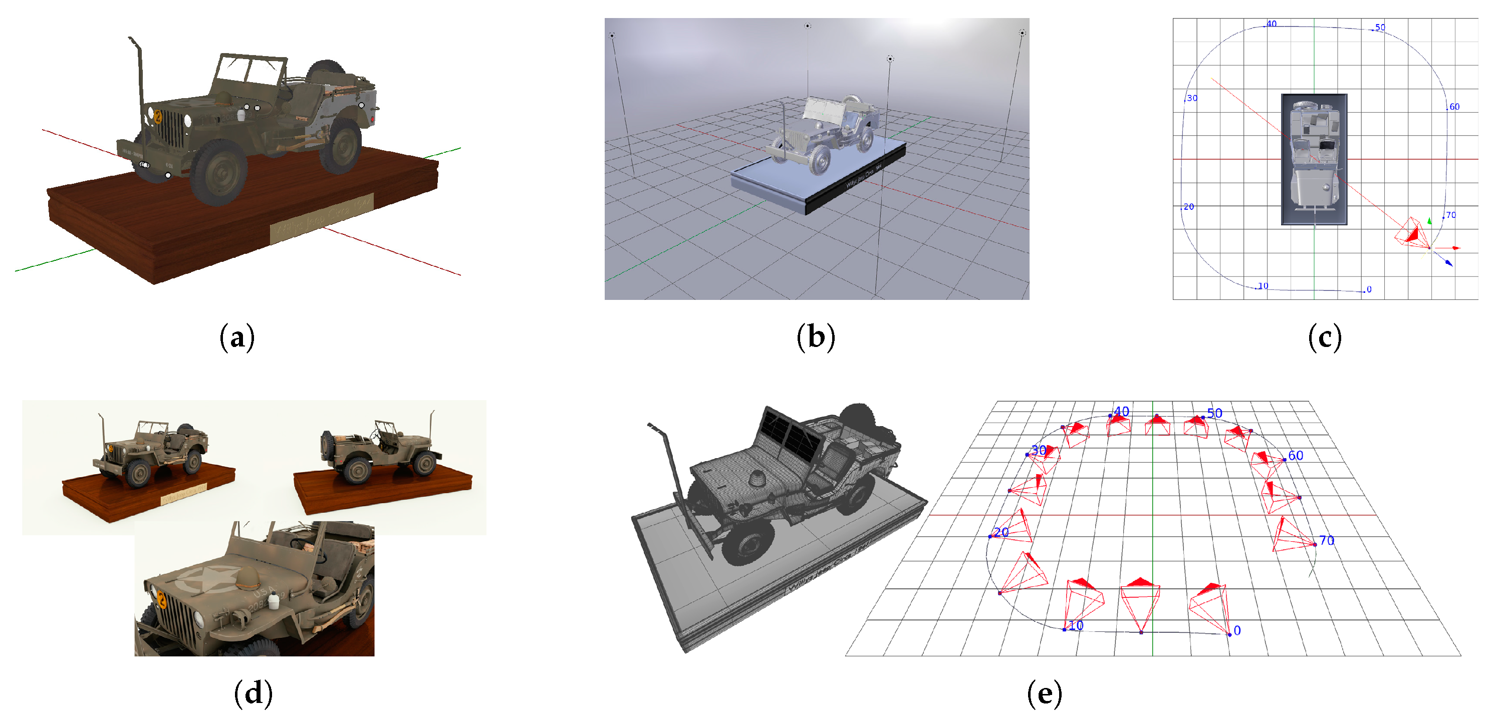
To overcome the problems in creating real datasets for evaluation, it is possible to use virtual 3D models to generate synthetic datasets with good image quality, intrinsic parameters for each image and optimal 3D model ground truth. With respect to real datasets usually acquired with physical imaging devices, the synthetic datasets make it possible to have accurate, and infinitely precise ground truths. We can generate synthetic datasets by acquiring images of virtual 3D models by means of rendering software. For our purposes we employ Blender [65]. First of all the subject of the dataset needs to be chosen; for optimal results the 3D model must have an highly detailed geometry and texture. It is also important that the model does not make use of rendering techniques like bump-map or normal-map; such features can simulate complex geometries in rendered images that are not defined in the model geometry, thus cannot be included when exporting the ground truth. The model must then be placed in a scene where lights and other objects can be included. A camera is then added and all its intrinsic calibration parameters must be set. Such camera is then animated to observe the scene from different view points; each frame of the animation will be used as an image of the dataset. Once everything is set the images can be rendered using Cycles, the Blender’s path-tracing render engine, that simulates light interactions and allows to generate photo-realistic images. Some EXIF metadata like focal length and sensor size can be added to the images so reconstruction pipelines can gather them automatically. Finally, along with the images, ground truth of model geometry and camera poses are needed. The ground truth geometry is the model itself, therefore it can be exported directly. Camera poses (position and orientation) can be obtained for each frame of the camera animation. Blender dose not have a direct way to export such information but it is easy to do that using its internal Python scripting framework. The entire flow of dataset generation is shown in Figure 3.

Synthetic dataset creation, pipeline execution and results evaluation involve many steps and various algorithms. To help the user in the process we created a plug-in for Blender that allows synthetic datasets generation and SfM reconstructions evaluation [66]. Such tool adds a simple panel in Blender’s user interface that makes possible to:

• import the main object of the reconstruction and setup a scene with lights for illumination and uniform background walls. Also, the parameters for the path tracing rendering engine are set.
• add a camera and setup its intrinsic calibration parameters. Animate the camera using circular rotations around the object to observe the scene from different view points.
• render the set of images and add EXIF metadata of intrinsic camera parameters used by SfM pipelines.
• eventually, geometry ground truth can be exported. This is not necessary if next steps are processed using this plug-in as the current scene will be used as ground truth.
• run the SfM pipelines listed in Section 2.2.
• import the reconstructed point cloud form SfM output and allow the user to manually eliminate parts that do not belong to the main object of the reconstruction.
• align the reconstructed point cloud to the ground truth using the Iterative Closest Point algorithm (ICP).
• evaluate the reconstructed cloud by computing the distance between the cloud and the ground truth and generating statistical information like min, max and average distance values and also reconstructed point count.

The dataset generation process could be used to create set of images of scene with various scale and likely include many objects, for those reason the plug-in divides the process in different steps, in this way it is possible for the user to adapt the result obtained after each step to specific needs. For example, it is possible to change the default camera intrinsic parameters, the scene illumination, animate the camera with different paths than the defaults and so on.

5. Experimental Results

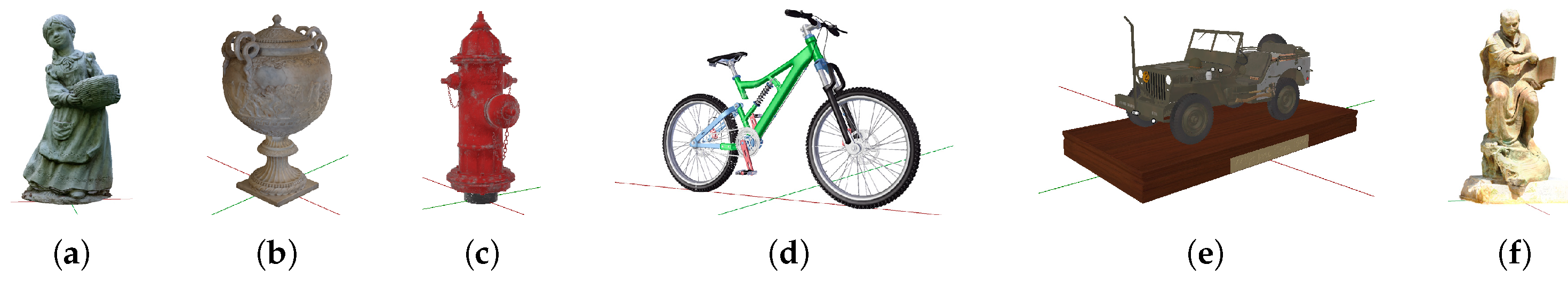
Five synthetic datasets of different 3D models (Figure 4) have been generated using the method described in Section 4:

• Statue [67]—set of images about a statue of height 10.01 m, composed of 121 images
• Empire Vase [68]—set of images about an ancient vase of height 0.92 m, composed of 86 images
• Bicycle [69]—set of images about a bicycle of height 2.66 m, composed of 86 images
• Hydrant [70]—set of images about an hydrant of height 1.00 m, composed of 66 images
• Jeep [71]—set of images about a miniature jeep of height 2.48 m, composed of 141 images

All the images of each dataset have been acquired at resolution 1920 × 1080 px using a virtual camera with a 35 mm focal length and 32 × 18 mm sensor. For every dataset is also generated the ground truth of object geometry and camera poses; in this way it is possible to run the reconstruction pipelines and evaluate the obtained results. In addition to our synthetic datasets the real dataset Ignatius (Figure 4f) from the “Tanks and Temples” collection [62] is also used, whose 263 images have been acquired at a resolution of 1920 × 1080 px. The physical height of the statue is 2.51 m. The datasets can be downloaded from [72].

Among all the SfM pipelines listed in Section 2.2 we compare the reconstructions results of COLMAP, Theia, OpenMVG and VisualSFM because each one is a reference implementation. In particular VisualSFM and COLMAP represent two remarkable developments of the incremental SfM pipeline with improvements in accuracy and performance compared to previous state-of-the-art implementations. Theia and OpenMVG are instead two ready to use SfM and multi-view geometry libraries that implement reconstruction algorithms and allow to build SfM pipelines that meet specific needs.

In order to evaluate dense 3D reconstructions, we paired the chosen SfM pipeline with CMVS/PMVS [73,74] as our MSV reference algorithm because it is widely used state-of-the-art implementation and is also natively supported by all the SfM pipelines used. The use of a single MVS pipeline with the same configuration parameters for all the reconstructions allows to evaluate and compare the dense results based on the quality os the sparse SfM reconstruction. In such way no other variables affect the reconstruction process. Here, we reported the results of evaluations done using method described in Section 3. Results are reported in

Table 2. SfM cloud evaluation results. $\overline{x}$ is the average distance of the point cloud from the ground truth and s its standard deviation. $N_p$ is the number of reconstructed points.

Model	COLMAP			OpenMVG			Theia			VisualSFM
	$\overline{\mathit{x}}$ [m]	s [m]	${\mathit{N}}_{\mathit{p}}$	$\overline{\mathit{x}}$ [m]	s [m]	${\mathit{N}}_{\mathit{p}}$	$\overline{\mathit{x}}$ [m]	s [m]	${\mathit{N}}_{\mathit{p}}$	$\overline{\mathit{x}}$ [m]	s [m]	${\mathit{N}}_{\mathit{p}}$
Statue	0.034	0.223	9k	0.057	0.267	4k	0.020	0.039	8k	0.185	0.236	6k
Empire Vase	0.005	0.152	8k	0.013	0.191	2k	0.002	0.005	8k	0.007	0.013	5k
Bicycle	0.042	0.365	5k	0.156	1.705	7k	0.027	0.086	2k	0.056	0.796	4k
Hydrant	0.206	0.300	2k	–	–	28	0.045	0.123	89	0.029	0.032	1k
Jeep	0.053	1.058	6k	0.057	0.686	4k	0.012	0.016	8k	0.055	0.124	5k
Ignatius	0.009	0.021	23k	0.013	0.032	12k	0.023	0.022	10k	0.054	0.124	14k

,

Table 3. SfM camera pose evaluation results. $N_c$ is the percentage of used cameras. $\overline{x}$ is the mean distance from ground truth of reconstructed camera positions and $s_x$ its standard deviation. $\overline{r}$ is the mean rotation difference from ground truth of reconstructed camera orientations and $s_r$ its standard deviation. n.a. means measure not available.

Model	COLMAP					OpenMVG					Theia					VisualSFM
	${\mathit{N}}_{\mathit{c}}$	$\overline{\mathit{x}}$ [m]	${\mathit{s}}_{\mathit{x}}$ [m]	$\overline{\mathit{r}}$ [${}^{\circ }$]	${\mathit{s}}_{\mathit{r}}$ [m]	${\mathit{N}}_{\mathit{c}}$	$\overline{\mathit{x}}$ [m]	${\mathit{s}}_{\mathit{x}}$ [m]	$\overline{\mathit{r}}$ [${}^{\circ }$]	${\mathit{s}}_{\mathit{r}}$ [m]	${\mathit{N}}_{\mathit{c}}$	$\overline{\mathit{x}}$ [m]	${\mathit{s}}_{\mathit{x}}$ [m]	$\overline{\mathit{r}}$ [${}^{\circ }$]	${\mathit{s}}_{\mathit{r}}$ [m]	${\mathit{N}}_{\mathit{c}}$	$\overline{\mathit{x}}$ [m]	${\mathit{s}}_{\mathit{x}}$ [m]	$\overline{\mathit{r}}$ [${}^{\circ }$]	${\mathit{s}}_{\mathit{r}}$ [m]
Statue	100	0.08	0.01	0.04	0.05	100	0.27	0.03	0.47	0.22	100	1.86	0.09	0.45	0.22	100	1.45	0.91	3.55	2.88
E. Vase	100	0.01	0.01	0.51	0.05	83	0.78	1.62	32.19	64.89	100	0.13	0.07	0.91	0.35	94	0.15	0.14	4.91	5.07
Bicycle	88	0.04	0.02	0.25	0.19	94	0.60	1.09	7.00	12.53	37	0.60	0.03	1.10	0.31	47	0.27	0.14	1.32	1.03
Hydrant	82	2.63	2.09	72.28	64.98	3	–	–	–	–	6	3.49	0.29	174.27	0.51	80	2.43	1.76	66.29	58.90
Jeep	63	0.04	0.02	0.26	0.11	92	0.24	1.32	4.80	26.33	95	0.43	0.42	1.33	5.67	83	1.02	2.79	9.68	22.84
Ignatius	100	n.a.	n.a.	n.a.	n.a.	100	n.a.	n.a.	n.a.	n.a.	100	n.a.	n.a.	n.a.	n.a.	100	n.a.	n.a.	n.a.	n.a.

,

Table 4. MVS cloud evaluation results. $\overline{x}$ is the average distance of the point cloud from the ground truth and s its standard deviation. ${{N}}_{{p}}$ is the number of reconstructed points.

Model	COLMAP			OpenMVG			Theia			VisualSFM
	$\overline{\mathit{x}}$ [m]	s [m]	${\mathit{N}}_{\mathit{p}}$	$\overline{\mathit{x}}$ [m]	s [m]	${\mathit{N}}_{\mathit{p}}$	$\overline{\mathit{x}}$ [m]	s [m]	${\mathit{N}}_{\mathit{p}}$	$\overline{\mathit{x}}$ [m]	s [m]	${\mathit{N}}_{\mathit{p}}$
Statue	0.009	0.023	75k	0.008	0.027	86k	0.010	0.011	84k	0.065	0.049	76k
Empire Vase	0.001	0.001	390k	0.001	0.004	246k	0.002	0.002	356k	0.005	0.007	240k
Bicycle	0.013	0.012	74k	0.062	0.146	69k	0.018	0.020	46k	0.021	0.025	44k
Hydrant	0.008	0.017	42k	–	–	–	0.080	0.147	11k	0.008	0.014	40k
Jeep	0.010	0.016	236k	0.008	0.016	471k	0.014	0.019	448k	0.048	0.056	281k
Ignatius	0.004	0.004	155k	0.003	0.004	161k	0.018	0.019	109k	0.017	0.031	76k

and

Table 5. Pipelines execution times in seconds and memory usage in MB.

Model	COLMAP				OpenMVG				Theia				VisualSFM
	SfM		MVS		SfM		MVS		SfM		MVS		SfM		MVS
	t [s]	$\mathit{RAM}$	t [s]	$\mathit{RAM}$	t [s]	$\mathit{RAM}$	t [s]	$\mathit{RAM}$	t [s]	$\mathit{RAM}$	t [s]	$\mathit{RAM}$	t [s]	$\mathit{RAM}$	t [s]	$\mathit{RAM}$
Statue	59	897	86	1062	43	1359	115	1300	196	1984	98	1249	86	1406	144	1452
Empire Vase	53	897	154	2101	28	628	130	1734	129	1988	134	1926	62	1226	159	2095
Bicycle	98	896	117	1356	57	1467	146	1720	63	1722	58	548	64	1226	68	641
Hydrant	19	894	55	793	16	1547	–	–	17	2048	3	1249	36	997	56	1452
Jeep	38	897	121	1812	69	1550	275	3209	213	2083	280	3293	109	1406	254	3078
Ignatius	1225	1825	430	5082	401	1555	494	5926	992	2588	484	5626	1639	2381	345	4742

and some examples of reconstructed dense point cloud are visible in

Table 6. Example of dense point clouds using CMVS/PMVS on different SfM reconstructions.

	COLMAP	OpenMVG	Theia	VisualSFM
Statue
Empire Vase
Bicycle
Hydrant		n.a.
Jeep
Ignatius

.

SfM pipelines have generated sufficient information to allow dense reconstruction on all datasets except for the Hydrant one. That dataset has a low geometric complexity, an high level of symmetry and an almost uniform texture; for these reasons SfM pipelines were not able to find enough correspondence between images and thus cannot generate a good reconstruction. The worst result was obtained with the OpenMVG pipeline and was not possible to run the MVS pipeline. COLMAP is the pipeline that achieves better results on average; even when it does not generate the best reconstruction it achieves good results.

Results for dataset Ignatius do not include camera pose evaluation because no information about camera pose ground truth is included in the dataset. This real dataset includes many elements besides the main object of the reconstruction; for this reason the reconstructed clouds have an high number of points that do not belong to the statue and thus must be removed. An evaluation of system resources usage was also done and COLMAP is efficient also in this aspect; using as much resources as possible it can complete the reconstruction in less time than the other pipelines.

The SfM reconstruction generated by pipeline Theia and dataset Statue shows that the obtained sparse point cloud is the best for that dataset but the camera poses are not accurate. These imprecisions are relative to camera positioning and not the camera rotation estimation that is instead always accurate. Further analysis shows that all the cameras are estimated positioned further away from the ground truth but on the correct viewing direction and for this reason the camera orientation is correct. Because the error in position is constant and applies to all the cameras this allows anyway the reconstruction of an accurate point cloud.

6. Conclusions

In this paper we analyzed the state-of-the-art incremental SfM pipelines showing that different algorithms and approaches can be used for each step of the reconstruction process. We proposed a complete method that starting from synthetic dataset generation allows to overcome real dataset limitations, evaluates and compares the reconstructions from different SfM implementations testing theirs limits under different conditions. The proposed method also allows to compare results after the MVS dense point cloud reconstruction. Our experiments results show that it is possible to generate synthetic datasets from which SfM reconstruction can successfully run obtaining satisfactory results. This also allows to take the pipelines to their limits showing that critical conditions can negatively affect the reconstruction process. To this end we have developed a plug-in for the Blender rendering software that allows us to generate synthetic datasets for the pipeline’s evaluation. Moreover, it simplifies the execution of the different steps of the evaluation procedure itself. With respect to real datasets usually acquired with physical imaging devices, the synthetic datasets make it possible to have accurate, and infinitely precise ground truths. According to our experiments, among the tested incremental SfM implementations, COLMAP showed the best average results. We also created a software tool that allows (in a single solution) to run the whole process, from the dataset generation to the reconstruction evaluation. Further work can be done to evaluate other aspects of the pipeline such as reconstructed object coverage to identify missing parts. The evaluation method can also be extended to include the subsequent mesh reconstruction and texture extraction phases.

References

- Poznanski, A. Visual Revolution of the Vanishing of Ethan Carter. 2014. Available online: http://www.theastronauts.com/2014/03/visual-revolution-vanishing-ethan-carter/ (accessed on 18 June 2018).
- Hamilton, A.; Brown, K. Photogrammetry and Star Wars Battlefront. 2016. Available online: https://www.ea.com/frostbite/news/photogrammetry-and-star-wars-battlefront (accessed on 18 June 2018).
- Saurer, O.; Fraundorfer, F.; Pollefeys, M. OmniTour: Semi-automatic generation of interactive virtual tours from omnidirectional video. In Proceedings of the 3DPVT2010 (International Symposium on 3D Data Processing, Visualization and Transmission), Paris, France, 17–20 May 2010. [Google Scholar]
- Nocerino, E.; Lago, F.; Morabito, D.; Remondino, F.; Porzi, L.; Poiesi, F.; Rota Bulo, S.; Chippendale, P.; Locher, A.; Havlena, M.; et al. A smartphone-based 3D pipeline for the creative industry-The replicate eu project. 3D Virtual Reconstr. Vis. Complex Arch. 2017, 42, 535–541. [Google Scholar] [CrossRef]
- Muratov, O.; Slynko, Y.; Chernov, V.; Lyubimtseva, M.; Shamsuarov, A.; Bucha, V. 3DCapture: 3D Reconstruction for a Smartphone. In Proceedings of the IEEE Conference on Computer Vision and Pattern Recognition Workshops, Las Vegas, NV, USA, 26 June–1 July 2016; pp. 75–82. [Google Scholar]
- SmartMobileVision. SCANN3D. Available online: http://www.smartmobilevision.com (accessed on 18 June 2018).
- Bernardini, F.; Bajaj, C.L.; Chen, J.; Schikore, D.R. Automatic reconstruction of 3D CAD models from digital scans. Int. J. Comput. Geom. Appl. 1999, 9, 327–369. [Google Scholar] [CrossRef]
- Izadi, S.; Kim, D.; Hilliges, O.; Molyneaux, D.; Newcombe, R.; Kohli, P.; Shotton, J.; Hodges, S.; Freeman, D.; Davison, A.; et al. KinectFusion: Real-time 3D reconstruction and interaction using a moving depth camera. In Proceedings of the 24th Annual ACM Symposium on User Interface Software and Technology, Santa Barbara, CA, USA, 16–19 October 2011; ACM: New York, NY, USA, 2011; pp. 559–568. [Google Scholar]
- Starck, J.; Hilton, A. Surface capture for performance-based animation. IEEE Comput. Graph. Appl. 2007, 27, 21–31. [Google Scholar] [CrossRef] [PubMed] [Green Version]
- Carlbom, I.; Terzopoulos, D.; Harris, K.M. Computer-assisted registration, segmentation, and 3D reconstruction from images of neuronal tissue sections. IEEE Trans. Med. Imaging 1994, 13, 351–362. [Google Scholar] [CrossRef] [PubMed]
- Noh, Z.; Sunar, M.S.; Pan, Z. A Review on Augmented Reality for Virtual Heritage System; Springer: Berlin/Heidelberg, Germany, 2009; pp. 50–61. [Google Scholar]
- Remondino, F. Heritage recording and 3D modeling with photogrammetry and 3D scanning. Remote Sens. 2011, 3, 1104–1138. [Google Scholar] [CrossRef] [Green Version]
- Özyeşil, O.; Voroninski, V.; Basri, R.; Singer, A. A survey of structure from motion. Acta Numer. 2017, 26, 305–364. [Google Scholar] [CrossRef]
- Schönberger, J.L.; Frahm, J.M. Structure-from-Motion Revisited. In Proceedings of the Conference on Computer Vision and Pattern Recognition (CVPR), Las Vegas, NV, USA, 26 June–1 July 2016. [Google Scholar]
- Ko, J.; Ho, Y.S. 3D Point Cloud Generation Using Structure from Motion with Multiple View Images. In Proceedings of the The Korean Institute of Smart Media Fall Conference, Kwangju, South Korea, 28–29 October 2016; pp. 91–92. [Google Scholar]
- Wu, C. Towards linear-time incremental structure from motion. In Proceedings of the 2013 International conference on IEEE 3D Vision-3DV 2013, Seattle, WA, USA, 29 June–1 July 2013; pp. 127–134. [Google Scholar]
- Snavely, N.; Seitz, S.M.; Szeliski, R. Photo tourism: Exploring photo collections in 3D. ACM Trans. Graph. (TOG) 2006, 25, 835–846. [Google Scholar] [CrossRef]
- Furukawa, Y.; Hernández, C. Multi-view stereo: A tutorial. Found. Trends Comput. Graph. Vis. 2015, 9, 1–148. [Google Scholar] [CrossRef]
- Fischler, M.A.; Bolles, R.C. Random sample consensus: A paradigm for model fitting with applications to image analysis and automated cartography. Commun. ACM 1981, 24, 381–395. [Google Scholar] [CrossRef]
- Hartley, R.; Zisserman, A. Multiple View Geometry in Computer Vision; Cambridge University Press: Cambridge, UK, 2003. [Google Scholar]
- Moons, T.; Van Gool, L.; Vergauwen, M. 3D reconstruction from multiple images part 1: Principles. Found. Trends Comput. Graph. Vis. 2010, 4, 287–404. [Google Scholar] [CrossRef]
- Triggs, B.; McLauchlan, P.F.; Hartley, R.I.; Fitzgibbon, A.W. Bundle adjustment—A modern synthesis. In International Workshop on Vision Algorithms; Springer: Berlin/Heidelberg, Germany, 1999; pp. 298–372. [Google Scholar]
- Schönberger, J.L.; Zheng, E.; Pollefeys, M.; Frahm, J.M. Pixelwise View Selection for Unstructured Multi-View Stereo. In Proceedings of the European Conference on Computer Vision (ECCV), Amsterdam, The Netherlands, 8–16 October 2016. [Google Scholar]
- Sweeney, C. Theia Multiview Geometry Library: Tutorial & Reference. Available online: http://theia-sfm.org (accessed on 30 July 2018).
- Moulon, P.; Monasse, P.; Marlet, R.; OpenMVG. An Open Multiple View Geometry Library. Available online: https://github.com/openMVG/openMVG (accessed on 30 July 2018).
- Wu, C. VisualSFM: A Visual Structure from Motion System. 2011. Available online: http://ccwu.me/vsfm/ (accessed on 30 July 2018).
- Wu, C.; Agarwal, S.; Curless, B.; Seitz, S.M. Multicore bundle adjustment. In Proceedings of the 2011 IEEE Conference on IEEE Computer Vision and Pattern Recognition (CVPR), Providence, RI, USA, 20–25 June 2011; pp. 3057–3064. [Google Scholar]
- Snavely, N.; Seitz, S.M.; Szeliski, R. Modeling the world from internet photo collections. Int. J. Comput. Vis. 2008, 80, 189–210. [Google Scholar] [CrossRef]
- Fuhrmann, S.; Langguth, F.; Goesele, M. MVE-A Multi-View Reconstruction Environment. In Proceedings of the Eurographics Workshop on Graphics and Cultural Heritage (GCH), Darmstadt, Germany, 6–8 October 2014; pp. 11–18. [Google Scholar]
- Zhao, L.; Huang, S.; Dissanayake, G. Linear SFM: A hierarchical approach to solving structure-from-motion problems by decoupling the linear and nonlinear components. ISPRS J. Photogramm. Remote Sens. 2018, 141, 275–289. [Google Scholar] [CrossRef]
- Lowe, D.G. Distinctive image features from scale-invariant keypoints. Int. J. Comput. Vis. 2004, 60, 91–110. [Google Scholar] [CrossRef]
- Gao, X.S.; Hou, X.R.; Tang, J.; Cheng, H.F. Complete solution classification for the perspective-three-point problem. IEEE Trans. Pattern Anal. Mach. Intell. 2003, 25, 930–943. [Google Scholar]
- Stewenius, H.; Engels, C.; Nistér, D. Recent developments on direct relative orientation. ISPRS J. Photogramm. Remote Sens. 2006, 60, 284–294. [Google Scholar] [CrossRef] [Green Version]
- Lepetit, V.; Moreno-Noguer, F.; Fua, P. Epnp: An accurate o (n) solution to the pnp problem. Int. J. Comput. Vis. 2009, 81, 155. [Google Scholar] [CrossRef] [Green Version]
- Agarwal, S.; Mierle, K. Ceres Solver. Available online: http://ceres-solver.org (accessed on 30 July 2018).
- Chum, O.; Matas, J. Matching with PROSAC-progressive sample consensus. In Proceedings of the Computer Society Conference on IEEE Computer Vision and Pattern Recognition (CVPR 2005), San Diego, CA, USA, 20–25 June 2005; Volume 1, pp. 220–226. [Google Scholar]
- Schönberger, J.L.; Price, T.; Sattler, T.; Frahm, J.M.; Pollefeys, M. A vote-and-verify strategy for fast spatial verification in image retrieval. In Asian Conference on Computer Vision; Springer: Cham, Switzerland, 2016; pp. 321–337. [Google Scholar]
- Chum, O.; Matas, J.; Kittler, J. Locally optimized RANSAC. In Joint Pattern Recognition Symposium; Springer: Berlin/Heidelberg, Germany, 2003; pp. 236–243. [Google Scholar]
- Alcantarilla, P.F.; Solutions, T. Fast explicit diffusion for accelerated features in nonlinear scale spaces. IEEE Trans. Pattern Anal. Mach. Intell. 2011, 34, 1281–1298. [Google Scholar]
- Muja, M.; Lowe, D. Fast Approximate Nearest Neighbors with Automatic Algorithm Configuration. In Proceedings of the VISAPP 2009—4th International Conference on Computer Vision Theory and Applications, Lisboa, Portugal, 5–8 February 2009; Volume 1, pp. 331–340. [Google Scholar]
- Cheng, J.; Leng, C.; Wu, J.; Cui, H.; Lu, H. Fast and accurate image matching with cascade hashing for 3D reconstruction. In Proceedings of the 2014 IEEE Conference on Computer Vision and Pattern Recognition (CVPR), Columbus, OH, USA, 23–28 June 2014; pp. 1–8. [Google Scholar]
- Rousseeuw, P.J. Least Median of Squares Regression. J. Am. Stat. Assoc. 1984, 79, 871–880. [Google Scholar] [CrossRef] [Green Version]
- Moisan, L.; Moulon, P.; Monasse, P. Automatic homographic registration of a pair of images, with a contrario elimination of outliers. Image Proc. On Line 2012, 2, 56–73. [Google Scholar] [CrossRef]
- Hesch, J.A.; Roumeliotis, S.I. A direct least-squares (DLS) method for PnP. In Proceedings of the 2011 IEEE International Conference on Computer Vision (ICCV), Barcelona, Spain, 6–13 November 2011; pp. 383–390. [Google Scholar]
- Lindstrom, P. Triangulation made easy. In Proceedings of the 2010 IEEE Conference on Computer Vision and Pattern Recognition (CVPR), San Francisco, CA, USA, 13–18 June 2010; pp. 1554–1561. [Google Scholar]
- Bujnak, M.; Kukelova, Z.; Pajdla, T. A general solution to the P4P problem for camera with unknown focal length. In Proceedings of the 2008 IEEE Conference on Computer Vision and Pattern Recognition (CVPR 2008), Anchorage, AK, USA, 23–28 June 2008; pp. 1–8. [Google Scholar]
- Hartley, R.I.; Sturm, P. Triangulation. Comput. Vis. Image Underst. 1997, 68, 146–157. [Google Scholar] [CrossRef]
- Raguram, R.; Frahm, J.M.; Pollefeys, M. A comparative analysis of RANSAC techniques leading to adaptive real-time random sample consensus. In Proceedings of the European Conference on Computer Vision, Marseille, France, 12–18 October 2008; Springer: Berlin/Heidelberg, Germany, 2008; pp. 500–513. [Google Scholar]
- Kukelova, Z.; Bujnak, M.; Pajdla, T. Real-time solution to the absolute pose problem with unknown radial distortion and focal length. In Proceedings of the 2013 IEEE International Conference on Computer Vision (ICCV), Sydney, Australia, 1–8 December 2013; pp. 2816–2823. [Google Scholar]
- Fragoso, V.; Sen, P.; Rodriguez, S.; Turk, M. EVSAC: accelerating hypotheses generation by modeling matching scores with extreme value theory. In Proceedings of the 2013 IEEE International Conference on Computer Vision (ICCV), Sydney, Australia, 1–8 December 2013; pp. 2472–2479. [Google Scholar]
- Arya, S.; Mount, D.M.; Netanyahu, N.S.; Silverman, R.; Wu, A.Y. An optimal algorithm for approximate nearest neighbor searching fixed dimensions. J. ACM 1998, 45, 891–923. [Google Scholar] [CrossRef] [Green Version]
- Lourakis, M.; Argyros, A. The Design and Implementation of a Generic Sparse Bundle Adjustment Software Package Based on the Levenberg-Marquardt Algorithm; Technical Report, Technical Report 340; Institute of Computer Science-FORTH: Heraklion, Greece, 2004. [Google Scholar]
- Bay, H.; Ess, A.; Tuytelaars, T.; Van Gool, L. Speeded-up robust features (SURF). Comput. Vis. Image Underst. 2008, 110, 346–359. [Google Scholar] [CrossRef]
- Tefera, Y.; Poiesi, F.; Morabito, D.; Remondino, F.; Nocerino, E.; Chippendale, P. 3DNOW: IMAGE-BASED 3D RECONSTRUCTION AND MODELING VIA WEB. Int. Arch. Photogramm. Remote Sens. Spat. Inf. Sci. 2018, 42, 1097–1103. [Google Scholar] [CrossRef]
- Horn, B.K. Closed-form solution of absolute orientation using unit quaternions. JOSA A 1987, 4, 629–642. [Google Scholar] [CrossRef]
- Girardeau-Montaut, D. CloudCompare (Version 2.8.1) [GPL Software]. 2017. Available online: http://www.cloudcompare.org/ (accessed on 18 June 2018).
- Besl, P.J.; McKay, N.D. Method for Registration of 3-D Shapes; Sensor Fusion IV: Control Paradigms and Data Structures; International Society for Optics and Photonics; Institute of Electrical and Electronics: New York, NY, USA, 1992; Volume 1611, pp. 586–607. [Google Scholar]
- Chen, Y.; Medioni, G. Object modelling by registration of multiple range images. Image Vis. Comput. 1992, 10, 145–155. [Google Scholar] [CrossRef]
- Rusinkiewicz, S.; Levoy, M. Efficient variants of the ICP algorithm. In Proceedings of the 2001 Third International Conference on 3-D Digital Imaging and Modeling, Quebec City, QC, Canada, 28 May–1 June 2001; pp. 145–152. [Google Scholar] [Green Version]
- Meagher, D.J. Octree enCoding: A New Technique for the Representation, Manipulation and Display of Arbitrary 3-d Objects by Computer; Electrical and Systems Engineering Department Rensseiaer Polytechnic Institute Image Processing Laboratory: New York, NY, USA, 1980. [Google Scholar]
- Eberly, D. Distance between Point and Triangle in 3D. Geometric Tools. 1999. Available online: https://www.geometrictools.com/Documentation/DistancePoint3Triangle3.pdf (accessed on 30 July 2018).
- Knapitsch, A.; Park, J.; Zhou, Q.Y.; Koltun, V. Tanks and Temples: Benchmarking Large-Scale Scene Reconstruction. ACM Trans. Graph. (TOG) 2017, 36, 78. [Google Scholar] [CrossRef]
- Zollhöfer, M.; Dai, A.; Innmann, M.; Wu, C.; Stamminger, M.; Theobalt, C.; Nießner, M. Shading-based refinement on volumetric signed distance functions. ACM ACM Trans. Graph. (TOG) 2015, 34, 96. [Google Scholar] [CrossRef]
- Seitz, S.M.; Curless, B.; Diebel, J.; Scharstein, D.; Szeliski, R. A comparison and evaluation of multi-view stereo reconstruction algorithms. In Proceedings of the 2006 IEEE Computer Society Conference on Computer Vision and Pattern Recognition, New York, NY, USA, 17–22 June 2006; Volume 1, pp. 519–528. [Google Scholar]
- Foundation, B. Blender. 1995. Available online: https://www.blender.org/ (accessed on 18 June 2018).
- Marelli, D.; Bianco, S.; Celona, L.; Ciocca, G. A Blender plug-in for comparing Structure from Motion pipelines. In Proceedings of the 2018 IEEE 8th International Conference on Consumer Electronics (ICCE), Berlin, Germany, 2–5 September 2018. [Google Scholar]
- Free 3D User Dgemmell1960. Statue. 2017. Available online: https://free3d.com/3d-model/statue-92429.html (accessed on 18 June 2018).
- Blend Swap User Geoffreymarchal. Empire Vase. 2017. Available online: https://www.blendswap.com/blends/view/90518 (accessed on 18 June 2018).
- Blend Swap User Milkyduhan. BiCycle Textured. 2013. Available online: https://www.blendswap.com/blends/view/67563 (accessed on 18 June 2018).
- Blend Swap User b82160. High Poly Hydrant. 2017. Available online: https://www.blendswap.com/blends/view/87541 (accessed on 18 June 2018).
- Blend Swap User BMF. Willys Jeep Circa 1944. 2016. Available online: https://www.blendswap.com/blends/view/82687 (accessed on 18 June 2018).
- Marelli, D.; Bianco, S.; Ciocca, G. Available online: http://www.ivl.disco.unimib.it/activities/evaluating-the-performance-of-structure-from-motion-pipelines/ (accessed on 18 June 2018).
- Furukawa, Y.; Ponce, J. Accurate, Dense, and Robust Multi-View Stereopsis. IEEE Trans. Pattern Anal. Mach. Intell. 2010, 32, 1362–1376. [Google Scholar] [CrossRef] [PubMed]
- Furukawa, Y.; Curless, B.; Seitz, S.M.; Szeliski, R. Towards Internet-scale Multi-view Stereo. In Proceedings of the 2010 IEEE Computer Society Conference on Computer Vision and Pattern Recognition, San Francisco, CA, USA, 13–18 June 2010. [Google Scholar]
Figure 1.
3D reconstruction using Structure from Motion.
Figure 2.
Incremental Structure from Motion pipeline.
Figure 3.
Example of synthetic dataset generation steps: (a) 3D model. (b) Scene setup. (c) Camera motion around the object. (d) Images rendering. (e) 3D model geometry and camera pose ground truth export.
Figure 4.
3D models used for synthetic dataset generation and Ignatius ground truth: (a) Statue [67]. (b) Empire Vase [68]. (c) Hydrant [70]. (d) Bicycle [69]. (e) Jeep [71]. (f) Ignatius [62].