
Nonlinear Adaptive Control with Asymmetric Pressure Difference Compensation of a Hydraulic Pressure Servo System Using Two High Speed On/Off Valves


1
National Research Center of Pumps, Jiangsu University, Zhenjiang 212013, China
2
College of Mechanical and Electrical Engineering, Nanjing University of Aeronautics and Astronautics, Nanjing 210016, China
Machines 2022, 10(1), 66; https://doi.org/10.3390/machines10010066
Submission received: 28 December 2021
/
Revised: 13 January 2022
/
Accepted: 13 January 2022
/
Published: 17 January 2022
(This article belongs to the Special Issue Advanced Control of Industrial Electro-Hydraulic Systems)
Abstract
:A hydraulic pressure servo system based on two high-speed on/off valves (HSV) is a discontinuous system due to the discrete flow of HSV when driven by pulse width modulation (PWM) signal. Pressure variation in the testing chamber is determined by the flow rate difference between the charging and discharging HSV. In this paper, a pressure controller consisting of a differential PWM (DPWM) scheme, asymmetric pressure difference compensation (APDC) and nonlinear adaptive control (NAC) is proposed to precisely control the pressure. The DPWM scheme is designed to improve the resolution of the net flow rate into the testing chamber. Furthermore, due to the strong asymmetry between the charging and the discharging process, the APDC method is proposed to design the two initial duty cycles of the DPWM signal which help to balance its charging and discharging ability under different working pressure points. Since the pressure system is a nonlinear, uncertain system due to oil compression and leakage, the NAC is designed to calculate the control duty cycle of the DPWM signal, which is used to overcome the unmodeled dynamic and parameter uncertainties. Comparative experiments indicate that the proposed controller can ensure good pressure tracking performance and enhance system robustness under different working pressure points and tracking frequencies.
1. Introduction
Electro-hydraulic servo systems (EHSS) have been widely used in the field of aircraft, such as in flight control subsystems [1], landing gear control subsystems [2], aircraft brake subsystems [3], and clutch pressure control systems for helicopters [4], because of their high power-weight ratio, high precision, and high-frequency response. However, due to use of a proportional/servo valve, some inherent drawbacks are difficult to overcome, such as poor anti-pollution ability, null shift, high cost, and high power consumption [5].
Compared to a proportional/servo valve, a high speed on/off valve (HSV) has the advantages of high repeatability, low throttling loss, low cost, and high reliability [6,7,8]. Recently, the use of HSV instead of proportional/servo valves has become a trend. A digital fluid system combined with several HSVs is considered as an alternative to EHSS. For example, in Ref. [9], a novel pulse width modulation (PWM) valve pulsing algorithm was designed to obtain linear velocity and a PID controller with friction compensation was used to achieve high precision position control of the pneumatic actuator. Lumkes et al. [10] designed a bang-bang controller, a phasing controller, and a fuzzy logic controller for an HSV-controlled position system. Their research results indicated that the phasing controller can achieve better tracking performance by using small and variable steps that can overcome the compressibility effect of hydraulic oil. In Ref. [11], two switching valves were used to control the speed of the hydraulic motor, and a sliding mode controller was designed to control the duty cycle of the PWM to overcome some parameter uncertainties. In the four HSV-controlled pneumatic servo systems, sixteen possible input combinations are presented and analyzed [12,13]. In the research, a novel seven-mode sliding controller was proposed to simultaneously improve the position accuracy of the actuator and reduce the switching number of the HSV. In a parallel on/off valve connected system, a PWM control scheme is often integrated into the pulse number modulation (PNM) controller to obtain higher flow resolution [14,15].
According to the above literature, many advanced control algorithms have been proposed for position servo control systems based on several HSVs. Moreover, in the pressure servo systems, Wang et al. [16,17] designed an HSV-controlled digital hydraulic pressure converter controller for high-pressure common rail and studied the relationship between the duty cycle and the output pressure of the converter. The research results indicate that the output pressure is almost proportional to the duty cycle of the input PWM signal. In automotive braking systems controlled by several HSVs [18,19], to overcome the modeling error and uncertainties, a sliding mode control based closed-loop algorithm scheme is often used to obtain accurate linear brake pressure. Jiao et al. [20] developed an integrated self-energized brake system for aircraft in which a 2/3 fast switching valve was used to control the pressure of the brake cylinder. In the research, a back-stepping controller is used to obtain robust performance. To improve the pressure tracking accuracy of a pneumatic servo system controlled by two fast-switching valves, Lin et al. [21] proposed a novel hybrid control strategy in which a time interlaced modulation and seven new possible control modes were designed to reduce the overshoot, the steady-state error and the settling time. In Ref. [22], an asymmetric structure comprising one HSV in the charging unit and three HSVs in the discharging unit were used to control the pressure in one chamber. In the research, a sliding mode controller with an asymmetric compensator was proposed to achieve high precision tracking of vacuum pressure.
The overall aim of this research is to accurately track the dynamic pressure via the use of two HSVs. A pressure controller consisting of a differential pulse width modulation (DPWM) scheme, asymmetric pressure difference compensation (APDC) and nonlinear adaptive control (NAC) is proposed. The DPWM is used to improve the resolution of the net flow rate into the testing chamber by regulating the difference between the duty cycles of the charging and discharging PWM. Moreover, the APDC is used to obtain a balance between the charging ability and discharging ability under different working pressures. The NAC scheme is used to eliminate the unmodeled dynamics and external disturbances. Extensive comparative simulations and experiments indicate that pressure tracking accuracy was significantly improved by the proposed pressure controller.
2. System Model and Characteristic Analysis
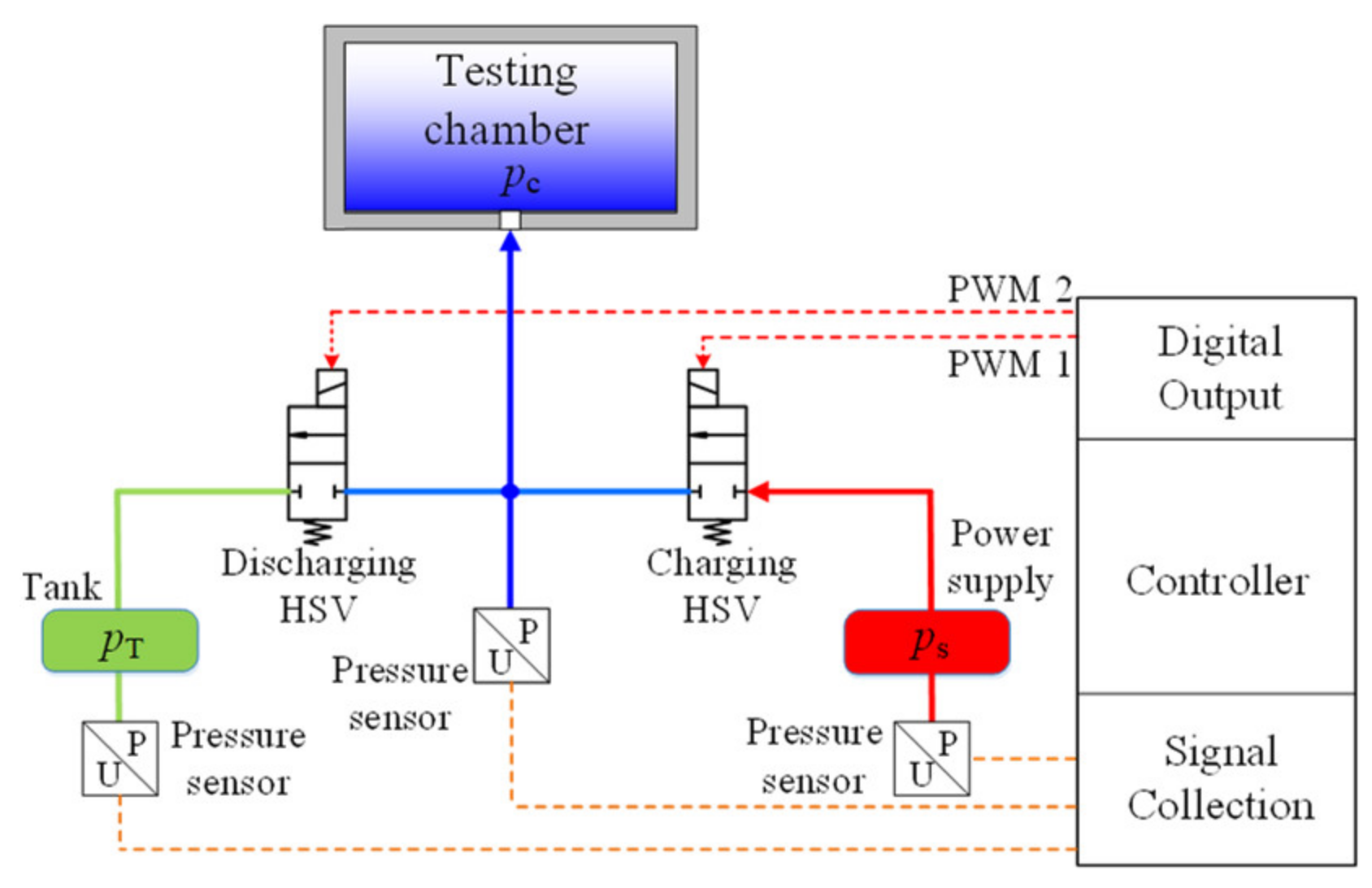
In this research, a pressure servo system based on two high speed on/off valves (HSVs) was used as the study object, as shown in Figure 1.
As shown in Figure 1, the testing chamber connects to the hydraulic power supply and tank via the charging HSV and the discharging HSV, respectively. When the charging HSV is energized, the oil flows into the testing chamber from the power supply which leads to the pressure in the testing chamber to rise. Conversely, when the discharging HSV is energized, the oil flows into the tank from the testing chamber, which leads the pressure in the testing chamber to drop.
Since the two HSVs are driven by the PWM signal, this produces the high-frequency discrete flow rate in the testing chamber, which makes the design of the pressure controller more difficult.
2.1. System Model
The mathematical model of the hydraulic pressure servo system consists of the pressure chamber model and the HSV flow model. Assuming that no leakage occurs in the chamber, the dynamic pressure model in the chamber can be written as [23]
where pc denotes the pressure of the testing chamber, denotes the average flow rate into the testing chamber, βe denotes the fluid bulk modulus, and Vc denotes the volume of the testing chamber.
The average flow rate into the testing chamber relates to the average flow rates of the two HSVs, and their relationship is defined as
where and denote the average flow rates of the charging HSV and the discharging HSV, respectively.
Since the charging HSV and the discharging HSV have same structure, the average flow rates of the two HSVs are calculated by
where Qh1 and Qh2 denote the flow rates of the charging HSV and the discharging HSV at the maximum opening, respectively. τ1 and τ2 denote the duty cycles of the two PWM signals which are used to drive the two HSVs. kq1 and kq2 denote the flow coefficients of the charging HSV and discharging HSV, respectively. ps and pt denote the supply pressure and return pressure, respectively.
2.2. HSV Performance
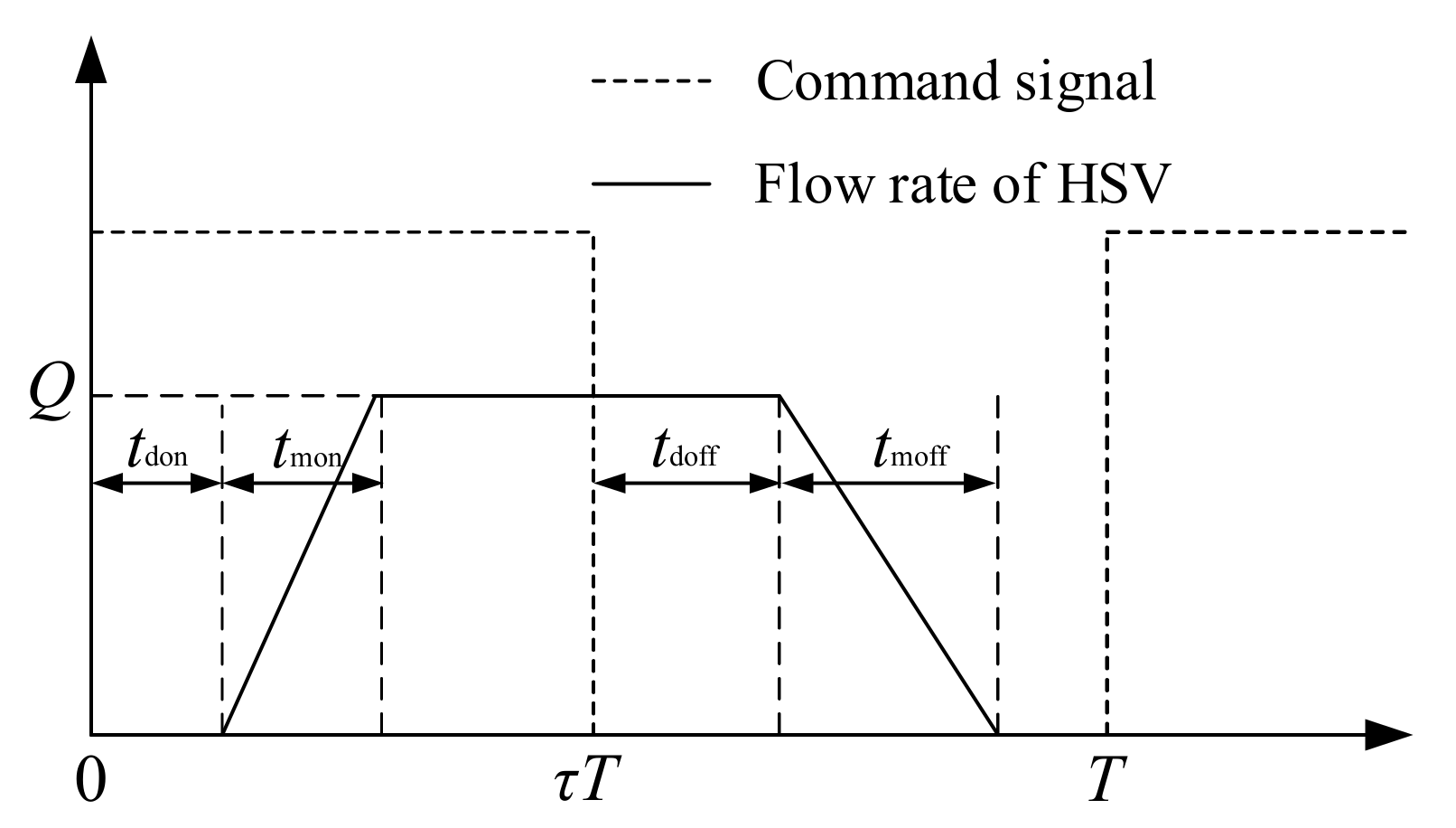
Due to the influences of electrical and mechanical hysteresis, the HSV suffers from a delay. The relationship between the flow rate and the command PWM signal is shown in Figure 2, where tdon denotes the opening delay time, tmon denotes the opening movement time tdoff denotes the closing delay time, and tmoff denotes the closing movement time.
As shown in Figure 2, the four critical time points (tdon, tmon, tdoff and tmoff) affect the effective range of the input duty cycle, which leads to an adverse effect on the control performance. In addition, the opening delay time tdon and the opening movement time tmon can be reduced by using the high driving voltage, and the closing delay time tdoff and the closing movement time tmoff are all reduced by using the negative voltage.
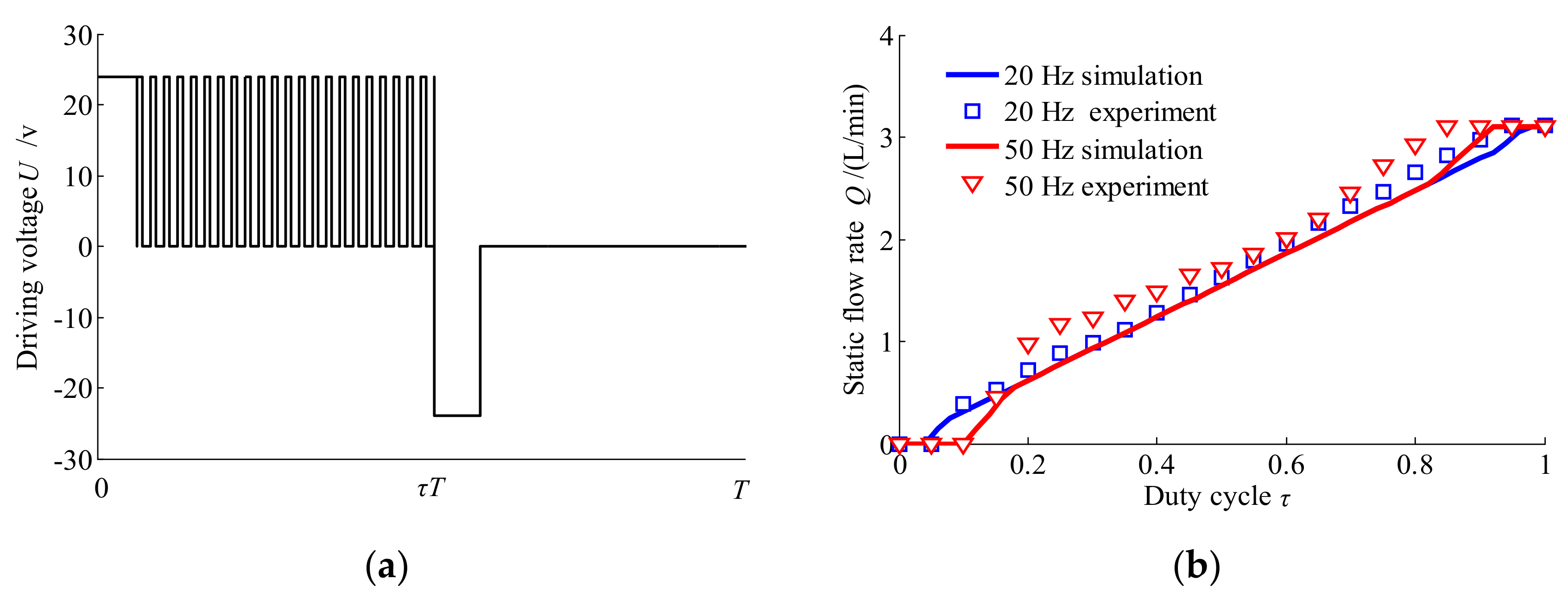
Therefore, the following adaptive PWM control signal (Figure 3a) [24] is often used to drive the HSV because of the several benefits, such as high dynamic performance and low power loss [25].
Figure 3b shows comparisons of the static flow rate between the simulations and experiments when HSV is driven by an adaptive PWM signal. The changing rules of the simulations are same as those of the experiments, although there exists an error due to the changing flow coefficient which is not considered in the simulations. In addition, it is easy to know that the linear region of the static flow rate is approximately in the range of 0.2–0.8, which is acceptable.
2.3. Characteristics of Charging and Discharging Process
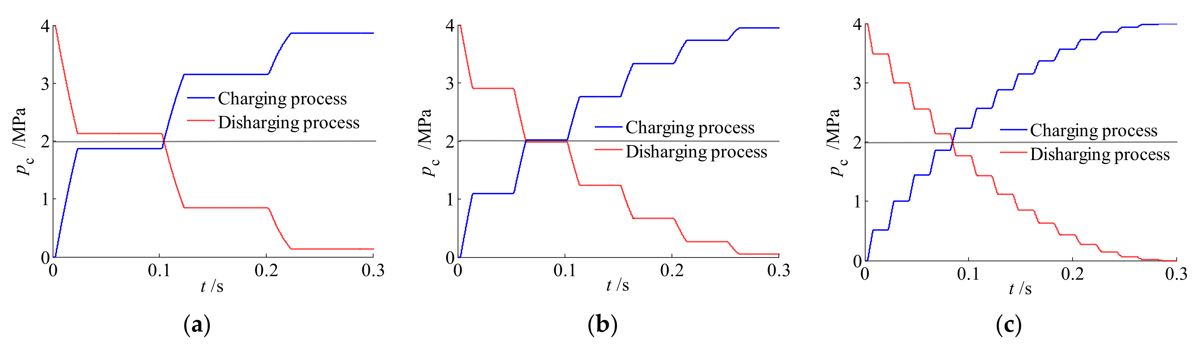
Simulation results of the charging and discharging characteristics under different switching frequencies are shown in Figure 4, in which the supply pressure was set 4 MPa.
As shown in Figure 4, the charging process and the discharging process are asymmetrical. For example, when the working pressure (pc) is smaller than half of the supply pressure, the charging speed is faster than the discharging speed. Conversely, when the working pressure (pc) is larger than half of the supply pressure, the charging speed is slower than the discharging speed.
In addition, the switching frequency has little effect on the charging and discharging speeds. However, with an increase to the switching frequency, the working pressure is more regulated, which is beneficial to improve the pressure tracking accuracy.
3. Pressure Controller Design
To achieve high precision control of the pressure tracking, a pressure controller was proposed which consists of a differential PWM scheme (DPWM), asymmetric pressure difference compensation (APDC) and a nonlinear adaptive control (NAC).
3.1. Differential PWM Scheme
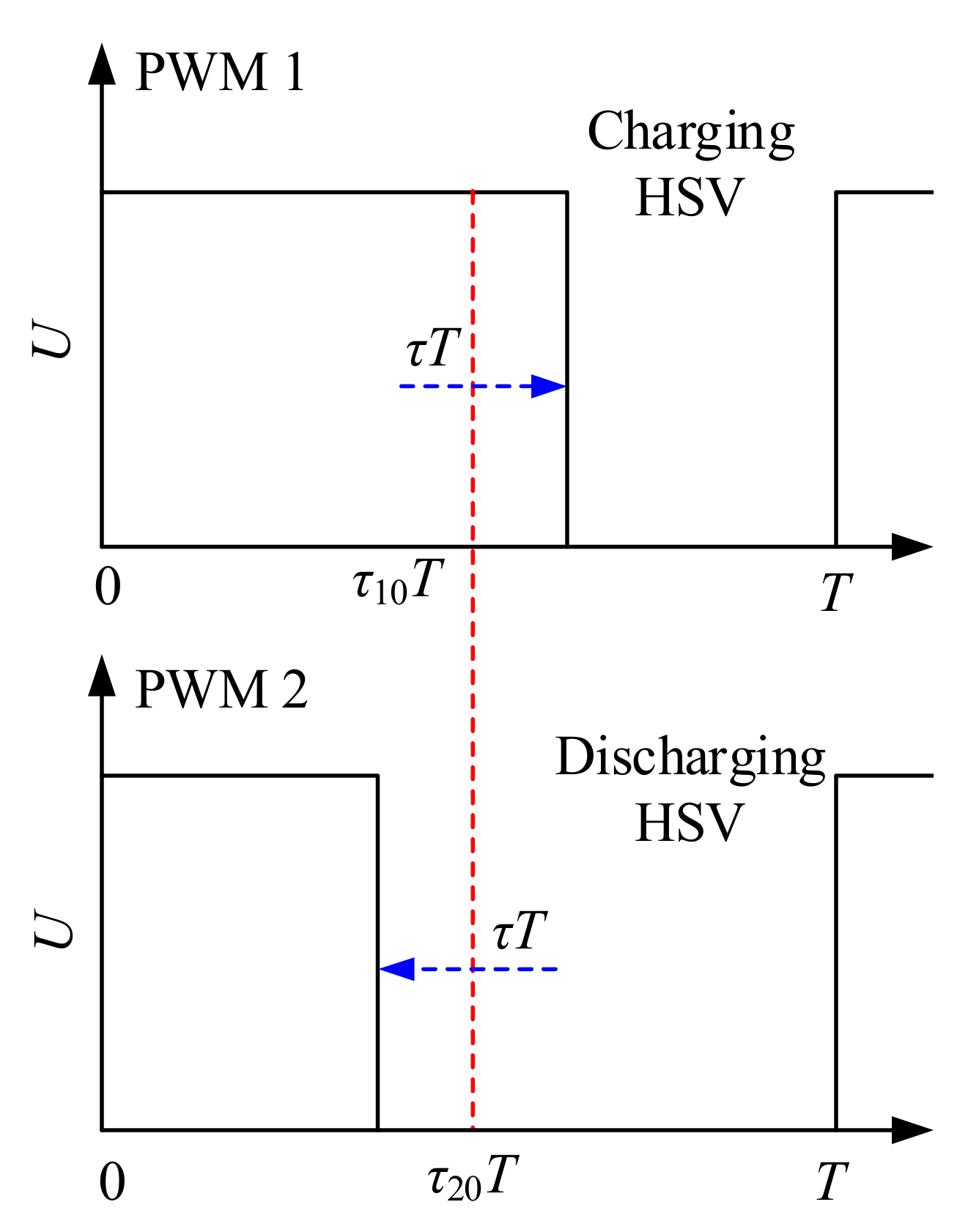
Considering the dead band and saturation of the HSV flow rate when driven by a conventional PWM signal, a differential PWM scheme was used to achieve the cross-flow between the charging HSV and the discharging HSV. The duty cycles of the differential PWM signals are shown in Figure 5, where U denotes the driving voltage, τ10 and τ20 denote the initial duty cycles of the PWM-1 and PWM-2 signals, respectively, τ denotes the control duty cycle, and T denotes the period of the PWM signal.
As shown in Figure 5, when the two HSVs are driven by the differential PWM signal, the cross-flow between the two HSVs is equal to the average flow rate of the chamber, so the following equation is achieved:
According to Equation (5), these parameters (τ10, τ20, and τ) are the key to achieving the accurate flow rate which is designed in the next section.
3.2. Asymmetric Pressure Difference Compensation (APDC)
The asymmetric pressure difference compensation scheme designed in this section was used to calculate the values of the initial duty cycles (τ10 and τ20) under the condition of the differential PWM scheme.
In previous publications [15,22,23], the values of the initial duty cycles were all selected as 0.5. This is because when the initial duty cycle is 0.5, the output flow rates of the two HSVs are the same, and better linearity of the flow rate is obtained.
However, in the pressure servo system, due to the coupling of the working pressure of the two HSVs, the design criteria of the initial duty cycle relate to the working pressures. For example, when the output flow rates of the two HSVs are the same, the following equation can be satisfied
To simplify the analysis, assuming that the two HSVs have the same opening area and flow coefficient, and the return pressure pt is ignored, so Equation (6) is simplified as
According to Figure 4 and Equation (7), the following conclusions are drawn:
- (a)
- When the working pressure pc is small (<ps/2), it means that the charging ability is stronger than the discharging ability because the pressure difference of the charging HSV is larger than that of the discharging HSV. To ensure that the charging ability equals the discharging ability, τ20 should be greater than τ10.
- (b)
- When the working pressure pc is moderate (=ps/2), it means that the charging ability is the same as the discharging ability because the pressure difference of the charging HSV is same as that of the discharging HSV. To ensure that the charging ability equals the discharging ability, τ20 equals τ10.
- (c)
- When the working pressure pc is large (>ps/2), it means that the charging ability is weaker than the discharging ability because the pressure difference of the charging HSV is smaller than that of the discharging HSV. To ensure that the charging ability equals the discharging ability, τ10 should be greater than τ20.
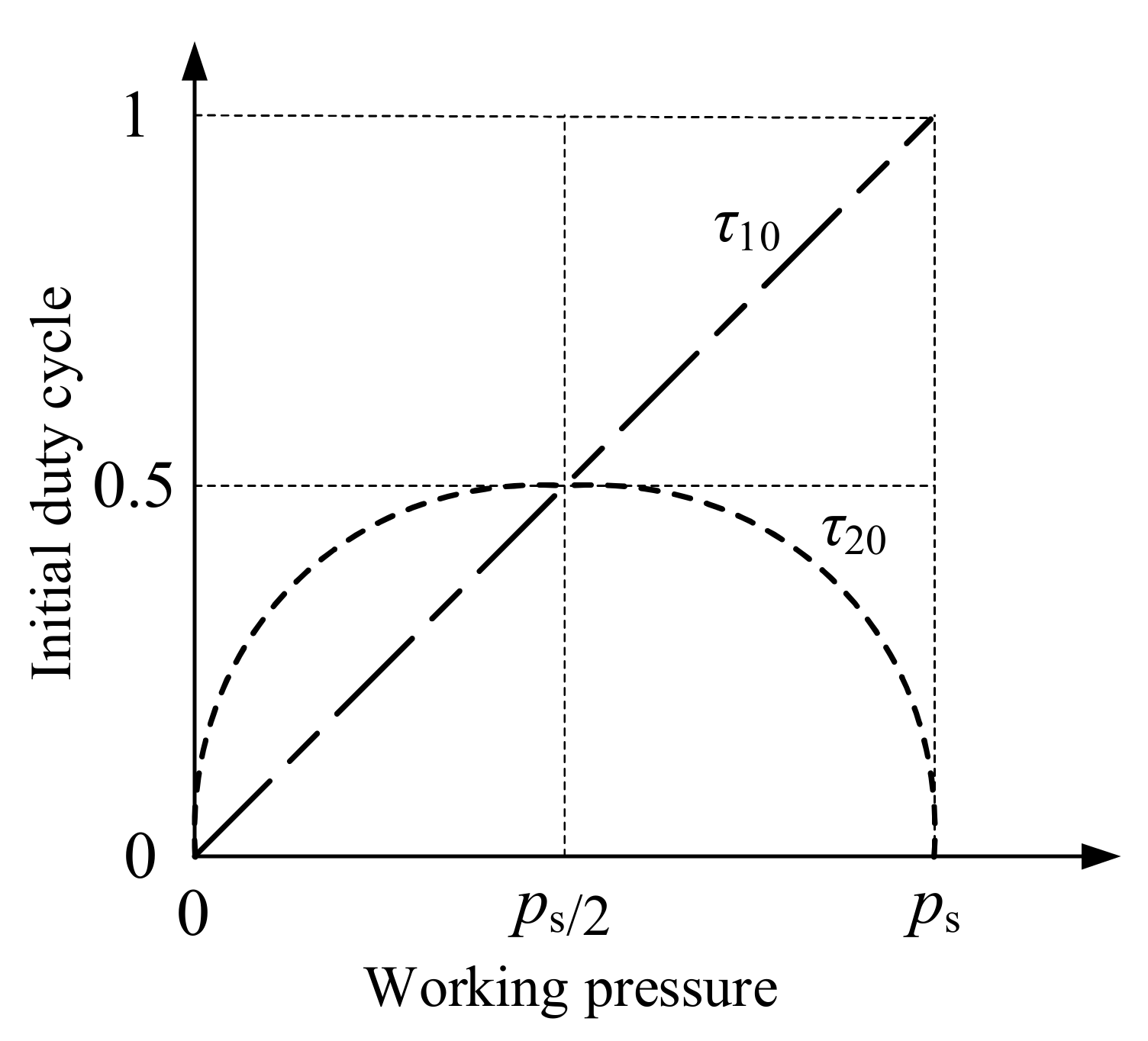
According to the above analysis, with the increase of the working pressure pc, the initial duty cycle τ10 of the charging HSV increases. The value of the τ10 is defined as
Substituting τ10 in Equation (8) into Equation (7), the initial duty cycle τ20 is obtained as follows
The functional mapping between the initial duty cycles and the working pressure is obtained based on the Equations (8) and (9), as shown in Figure 6.
3.3. NonlinearAdaptive Controller (NAC)
- (1)
- Controller design
A nonlinear adaptive controller designed in this section was used to calculate the control duty cycle τ. Assuming that the values of the βe and the Vc are known in this study, the mathematical model of the system considering the unmodeled dynamics and disturbances is written as [23]
where dn and denote the nominal value and the time-variant error of the unmodeled dynamics and disturbances, respectively.
Since the flow gain of the HSV is easily affected by pressure difference and oil viscosity, the relationship between the average flow rate in the chamber and the HSV is corrected as
where α denotes the uncertainty coefficient of the average flow rate into the testing chamber.
Define the unknown parameter set θ = [θ1, θ2]T, where θ1 = α, θ2 = dn, and also define the state variables as x = pc. Substituting Equation (11) into (10), the state-space equation can be formulated as
Assumption 1.
The parametric uncertainties and the time-variant error of the unmodeled dynamics and disturbances are all bounded, the following relation is satisfied.
The positive-definite Lyapunov function is defined as
where e denotes the pressure tracking error which is written as x − xd, and xd is the reference pressure tacking signal.
Taking the differentiate of Equation (14) with respect to time and substitute Equation (12) into it to obtain
Letting
where Qh denotes the difference between the average inflow and average outflow of the chamber, which is also selected as a virtual control input of the system, and the desired function Qhd is established for Qh as follows:
where Qhda1 and Qhda2 denote the stable compensation item and fast compensation item of the system, respectively, and Qhds1 and Qhds2 denote the linear stable feedback item and robust feedback item of the system, respectively.
Qhda1 and Qhds1 are defined as the following forms via parameter adaptation
where ks1 denotes the gain of the linear stable feedback item.
Substituting Equations (18) and (19) into Equation (17), it is easy to obtain
The relationship between the estimated value and the true value is as follows
Letting
where ζ and Δ are the nominal value and the time-variant error of the parametric uncertainties and nonlinear disturbance, respectively.
Qhda2 is designed as
where denotes the estimation of the fast dynamic compensation coefficient ζ which is estimated based on pressure error, as follows:
where and denote the maximum value and the minimum value of , respectively, and v denotes the adaptive law of the fast dynamic compensation coefficient ζ.
Substituting Equations (22) and (23) into Equation (20), it is easy to obtain
where is the estimation error of the fast dynamic compensation coefficient ζ.
The following boundary bounds :
where θ1m denotes the difference between the upper value and lower value of the estimated θ1, θ2m denotes the difference between the upper value and lower value of the estimated θ2, and dm is the absolute value of the maximum value of the high-frequency component of the uncertain nonlinearities.
To handle the modeling uncertainties, the robust term Qhds2 is designed as
where ε is the boundary layer thickness.
Substituting Equation (27) into Equation (25), we can obtain
According to Equation (28), the control system is stable and the pressure tracking error will converge to the sphere .
Combine Equations (18), (19), (23) and (27), the desired control input Qhd is as
According to Section 3.1, when the two HSVs are driven by the differential PWM, the following equation is satisfied
Substituting Qhd in Equation (29) into Equation (30), the control law (output duty cycle) can be obtained as
- (2)
- Parameter estimation and stability proof.
Due to using the constant value of the parameters’ estimates, it is difficult to maintain consistent control performance during the operation of the pressure system. To overcome the influences of the parametric uncertainties, the adaptive law is used to update the estimates online. The adaptive law of the uncertain parameters’ estimates is defined as:
where denotes the positive definite symmetric matrix of the adaptive law, and the ρ1 and ρ2 determine the update rate of the uncertain parameters. τp = [τp1 τp1]T denotes the adaptive function matrix. denotes the maximum update speed of the uncertain parameters. Sat(•) denotes the saturation function, which limits the update speed of the uncertain parameters.
The expressions of (•) and Sat(•) are defined as:
Therefore, the estimates of the uncertain parameters are bounded. The saturation function is used to avoid the system instability caused by faster update speeds of the uncertain parameters.
Based on the Lyapunov energy function, the following function is defined as
Taking the differentiate of Equation (35) with respect to time, the following equation is given [23]
To make < 0, the expression of and are defined as:
Substituting Equation (37) into Equation (36), we can obtain
Furthermore, integrating Equation (38) over [0, t], we can obtain
According to Equation (39), we can conclude that the system is stable, and ultimately bounded. This guarantees that the tracking error can converge to a small neighborhood of origin. Equation (39) also shows that a larger feedback gain ks1, and a smaller boundary layer thickness ε can produce a smaller steady-state error of the system.
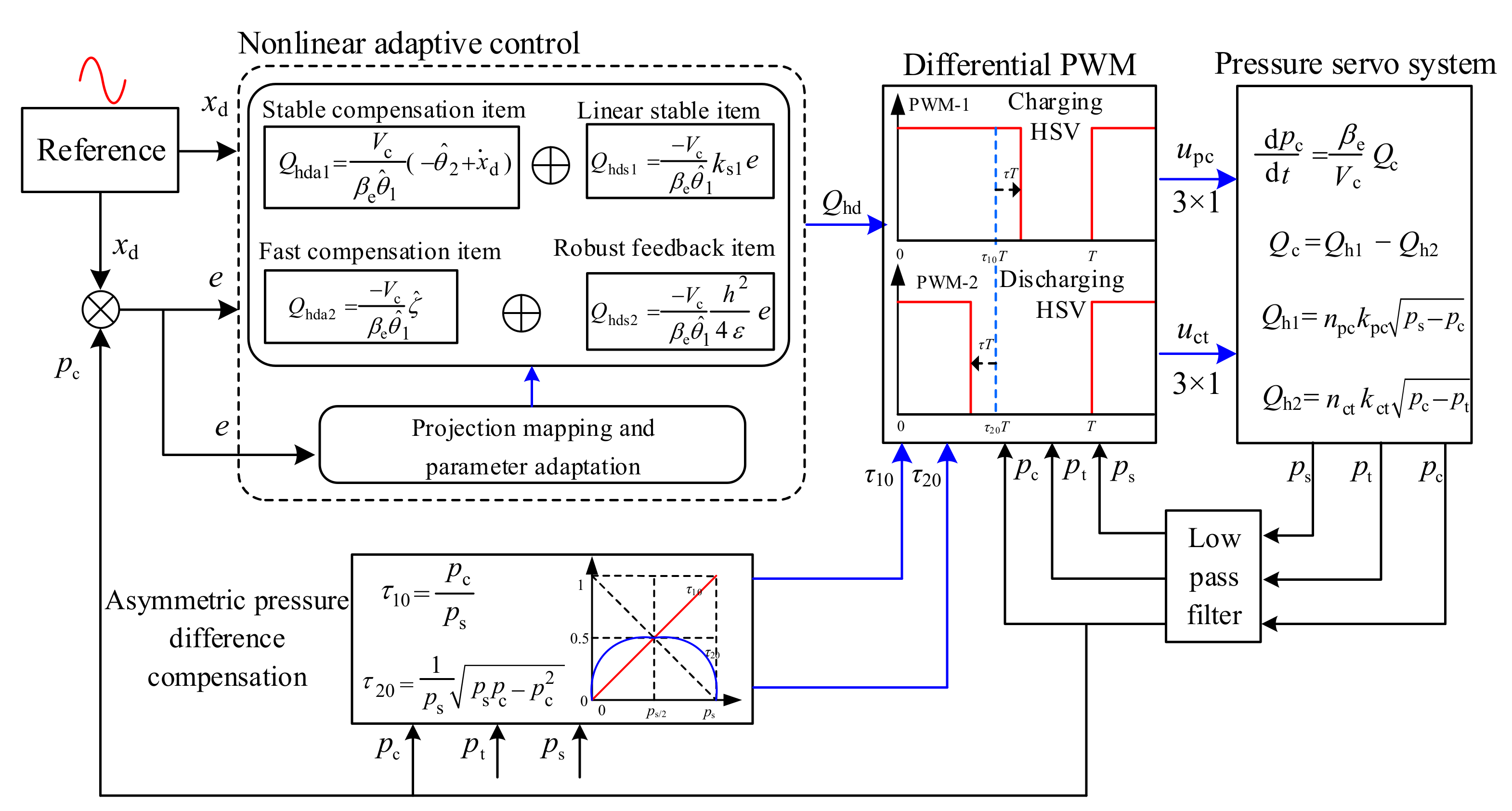
According to the above design of the differential PWM scheme, asymmetric pressure difference compensation, and the nonlinear adaptive controller, a diagram of the pressure control algorithm is shown in Figure 7.
4. Simulation Results
4.1. Open-Loop Control Characteristics
According to Equations (1) and (5), it is easy to obtain
Then
Substituting Equations (3), (4), (8) and (9) into Equation (41), the following equation is obtained
Therefore, the relationship between the control duty cycle τ and the desired control pressure pc is achieved. We can use the Equations (8), (9) and (42) to control the pressure in open-loop mode.
To compare the open-loop control and the NAC control in the simulation environment, the switching frequency of the HSV was set as 50 Hz, and the sampling time was set as 0.05 ms. The net flow into the chamber times a coefficient of 0.6 simulated the modelling uncertainties. The equivalent bulk modulus, density and kinematic viscosity of the oil were 700 MPa, 780 kg/m3, and 45 mm2/s, respectively. The rated pressure of the HSV was 10 MPa. The opening delay time, opening movement time, closing delay time, and closing movement time of the HSV were 2.2, 1.1, 3.3, and 1.2 ms, respectively. The flow coefficients of the charging HSV unit and the discharging HSV unit were both 3.9 × 10⁻⁹ m3/s.
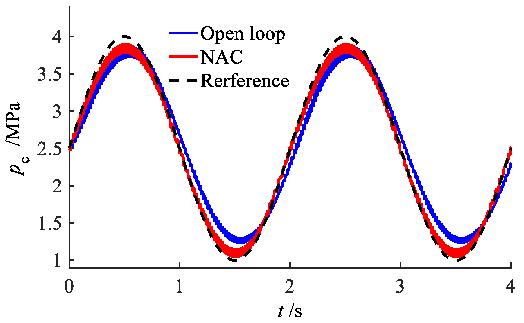
Figure 8 shows the comparisons between the open-loop control and the NAC control. When using the open-loop control, the pressure tracking curve had a large amount of lag and error compared to the command signal. This issue can be solved by using a NAC control in which a robust item is used to handle the modeling uncertainties. It is easy to find that when the pressure is in the region of the peak and trough of the sinusoidal signal, it still has large errors, which can be improved as described in the next section.
4.2. Tracking Performance of Different Controllers
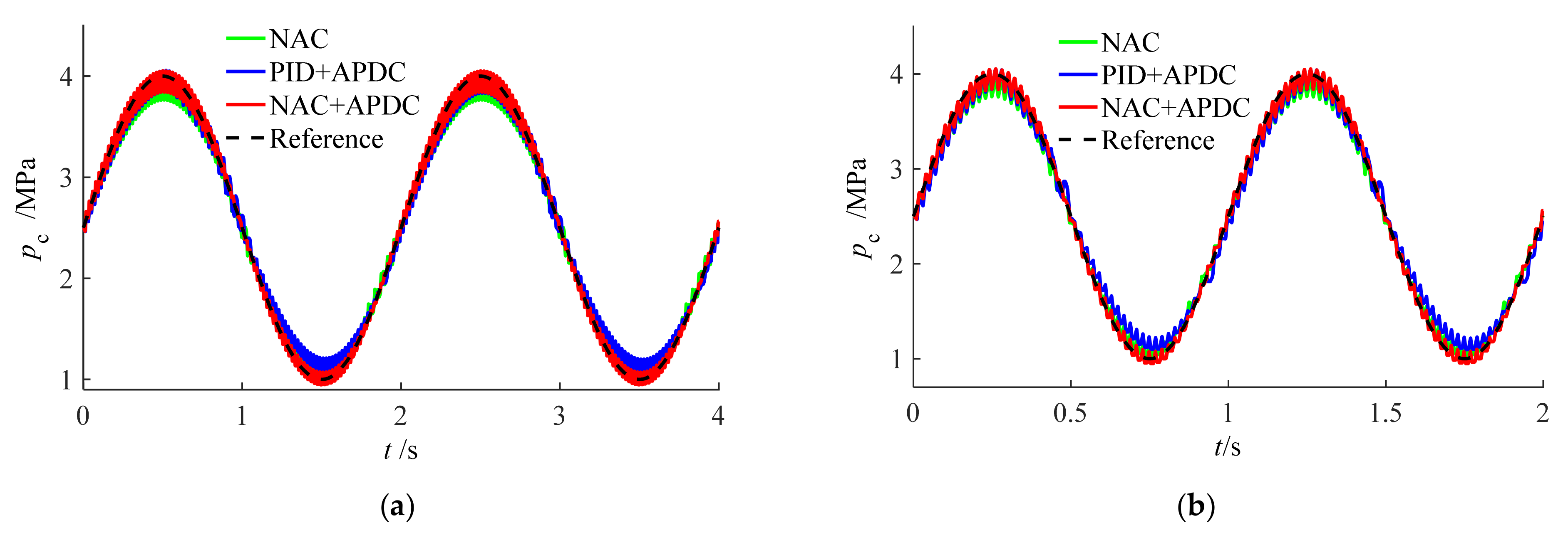
In order to validate the effectiveness of the proposed NAC + APDC controller, two other controllers (NAC and PID + APDC) were selected as the comparison objects. The reference signal for pressure tracking was a sinusoidal curve with different offset pressures (2.5 MPa, 2 MPa, and 1.5 MPa), and different frequencies (0.5 Hz and 1 Hz).
Simulation comparisons of the different controllers under different reference tracking signals are shown in Figure 9, Figure 10 and Figure 11, in which NAC denotes a nonlinear adaptive control, and NAC + APDC denotes the nonlinear adaptive control with asymmetric pressure difference compensation. The control parameters of the NAC + APDC controller were set to: , , , , ρ1 = 0.8, ρ2 = 10, ks1 = 180, and . The supply pressure was set as 4.5 MPa.
As can be seen from Figure 9, Figure 10 and Figure 11, when tracking the sinusoidal signal with different frequencies and different offset pressure points, the tracking performance of the NAC controller was basically consistent with that of the PID + APDC controller. These two controllers both show a poor tracking performance especially away from the middle offset pressure points, although while maintaining a good signal shape. Conversely, the proposed NAC + APDC controller maintained a better tracking performance.
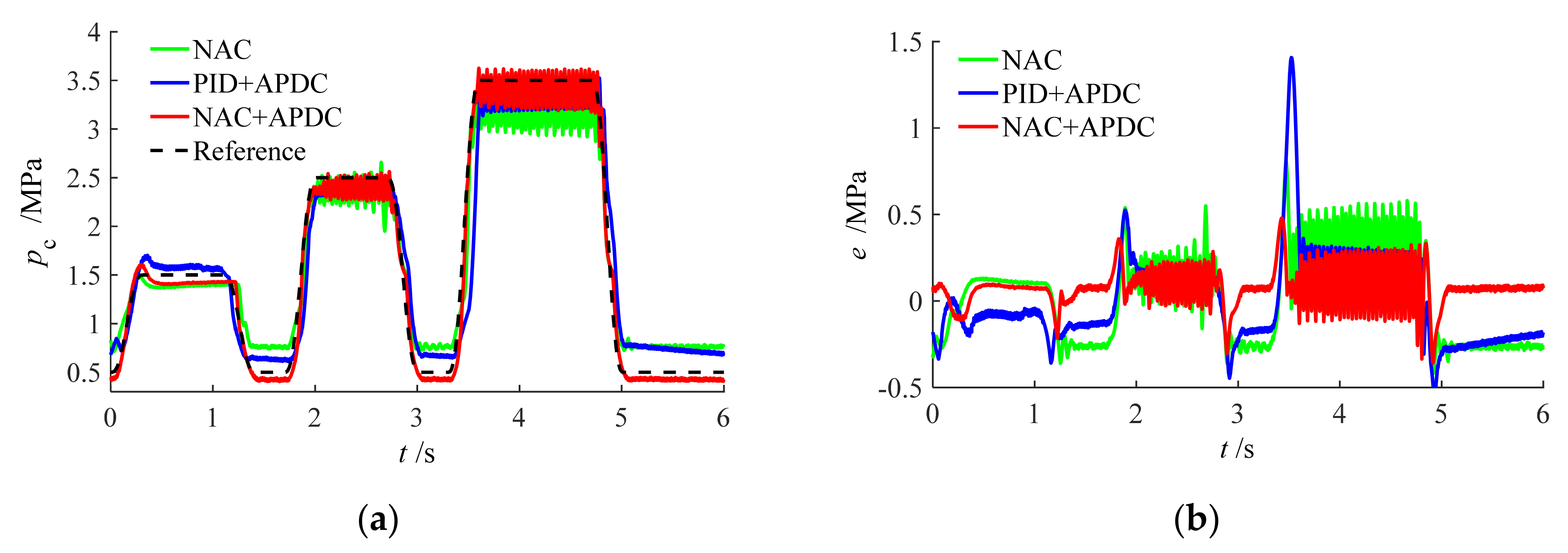
To test fixed pressure tracking performance, and considering that there are few sudden square signals in practical applications, a smooth square signal instead of a square wave was used as the pressure tracking signal. The simulation results of the smooth square pressure tracking signal under different controllers are shown in Figure 12.
As shown in Figure 12, compared to the controller PID + APDC, when using the proposed NAC + APDC controller, the tracking error of the fixed pressure was significantly reduced (<0.1 MPa) because the NAC + APDC controller adapted to changes to the different working pressure points and always selected the most suitable HSV operations to fulfil the best HSV operations.
5. Experimental Research
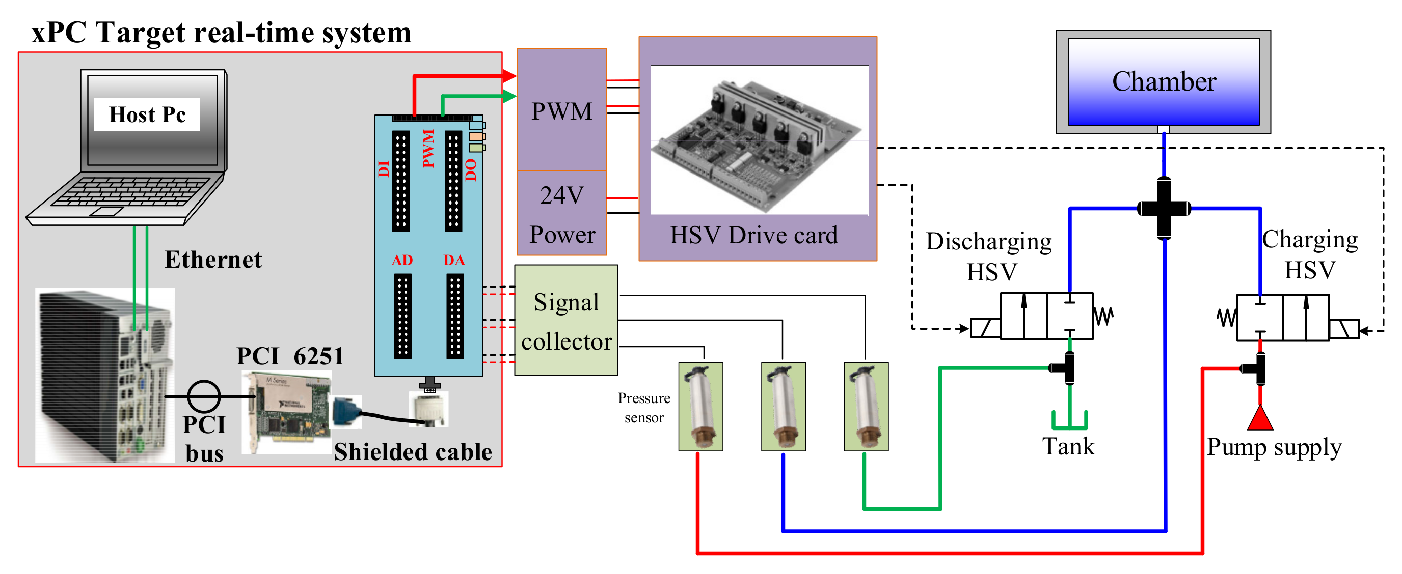
To verify the effectiveness of the proposed controller, comprehensive performance comparisons were conducted on a hydraulic test platform, as shown in Figure 13. The platform mainly consists of two high speed on/off valves, a testing chamber, two pressure sensors, a hydraulic supply of 10 MPa, and an xPC real-time control system. In the xPC real-time control system, a master and a slave computer are used to monitor and implement the designed controller, respectively. A data acquisition and control card was used to output the PWM control signal and collect the pressure signal. The 5 V PWM control signal needs to be amplified into a 24 V PWM signal by the HSV drive card which is powered by a 24 V DC. The high-frequency pressure sensors (response frequency of 20 kHz) were used to measure the pressure of the testing chamber and the supply pressure. The pressure in tank was assumed to be 0. To implement the designed controllers described above, a MATLAB/Simulink model needed to be compiled into discretized C++ codes.
5.1. Characteristics of Charging and Discharging Process
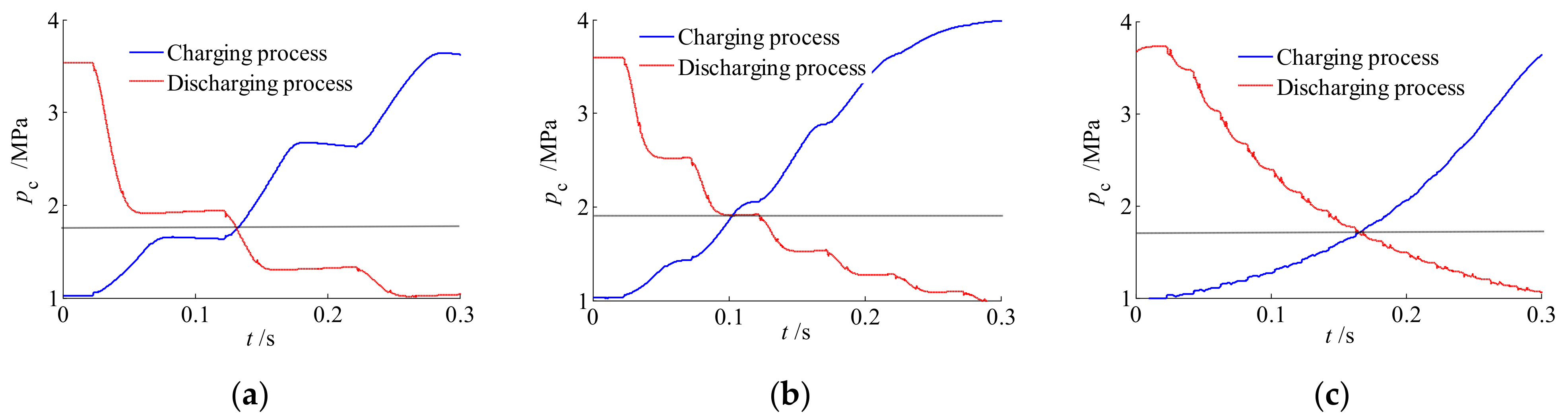
The experiments of the charging and discharging process are shown in Figure 14. The changing rules of the experimental results were the same as the simulations, where the charging and the discharging process are asymmetrical. That is, assuming that the two HSVs’ flow coefficients were same, when the working pressure is smaller than half of the supply pressure, the charging speed was faster than the discharging speed. Conversely, when the working pressure was greater than half of the supply pressure, the charging speed was slower than the discharging speed. When the working pressure was equal to the half of the supply pressure, the charging speed was same as the discharging speed.
5.2. Tracking Performance of Different Controllers
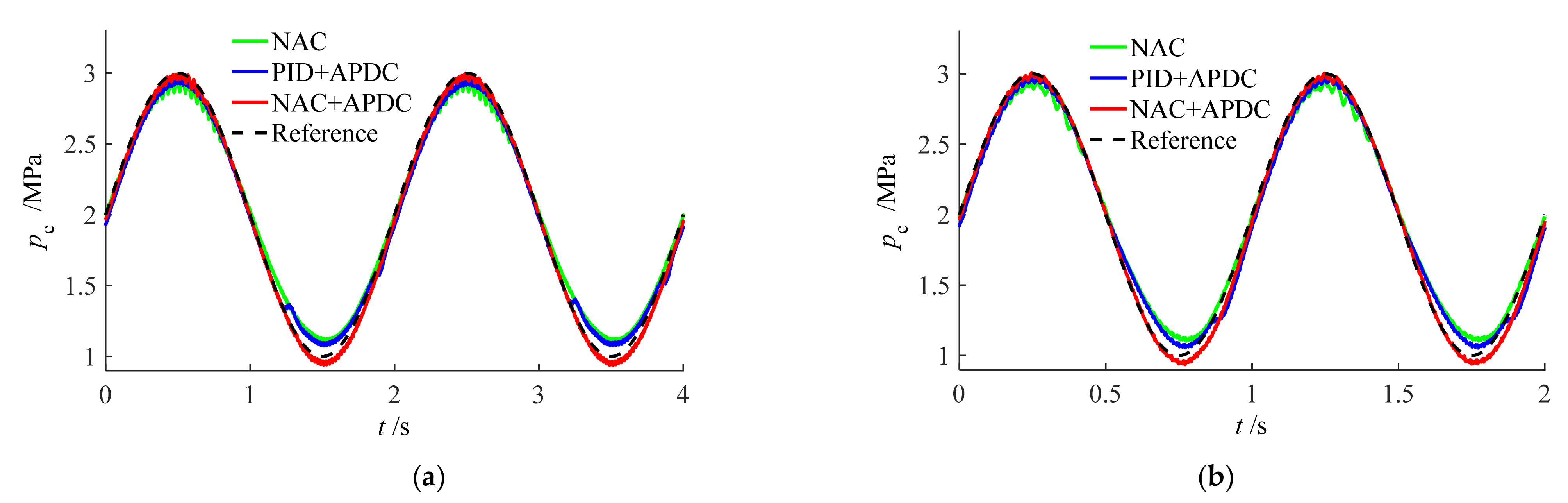
Experimental comparisons of the different controllers under different reference tracking signals are shown in Figure 15, Figure 16 and Figure 17. Control parameters in experiments are the same as that in simulations. The flow coefficients of the charging HSV unit and the discharging HSV unit are both 3.9 × 10⁻⁹ m3/s.
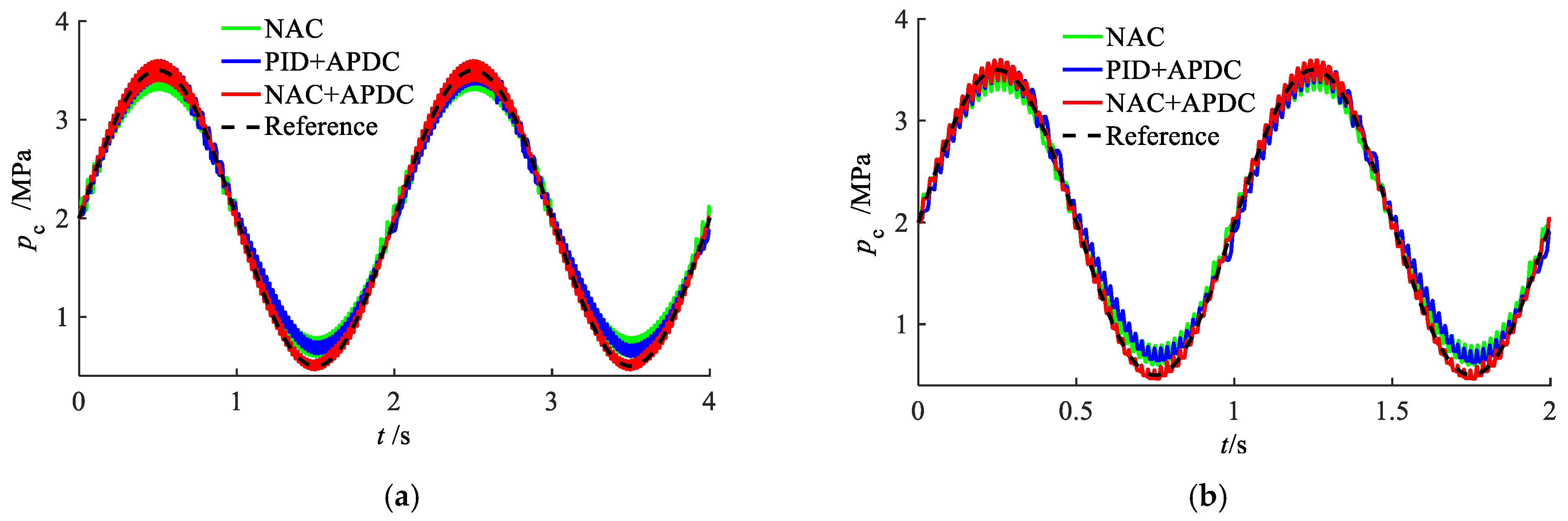
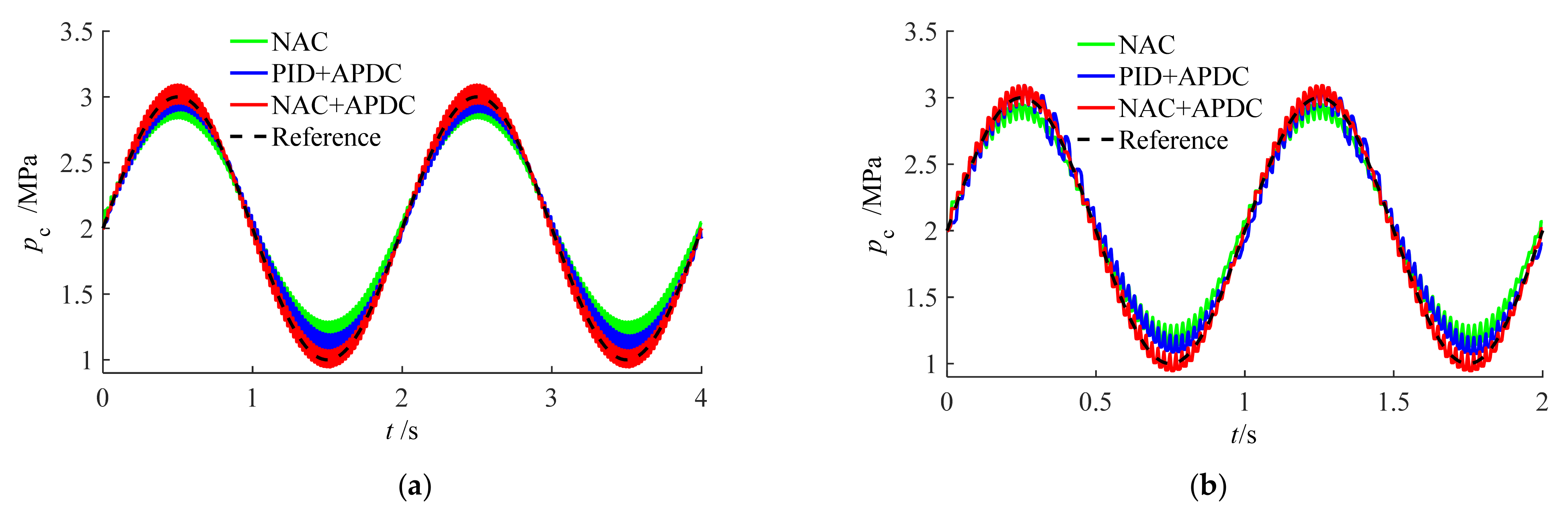
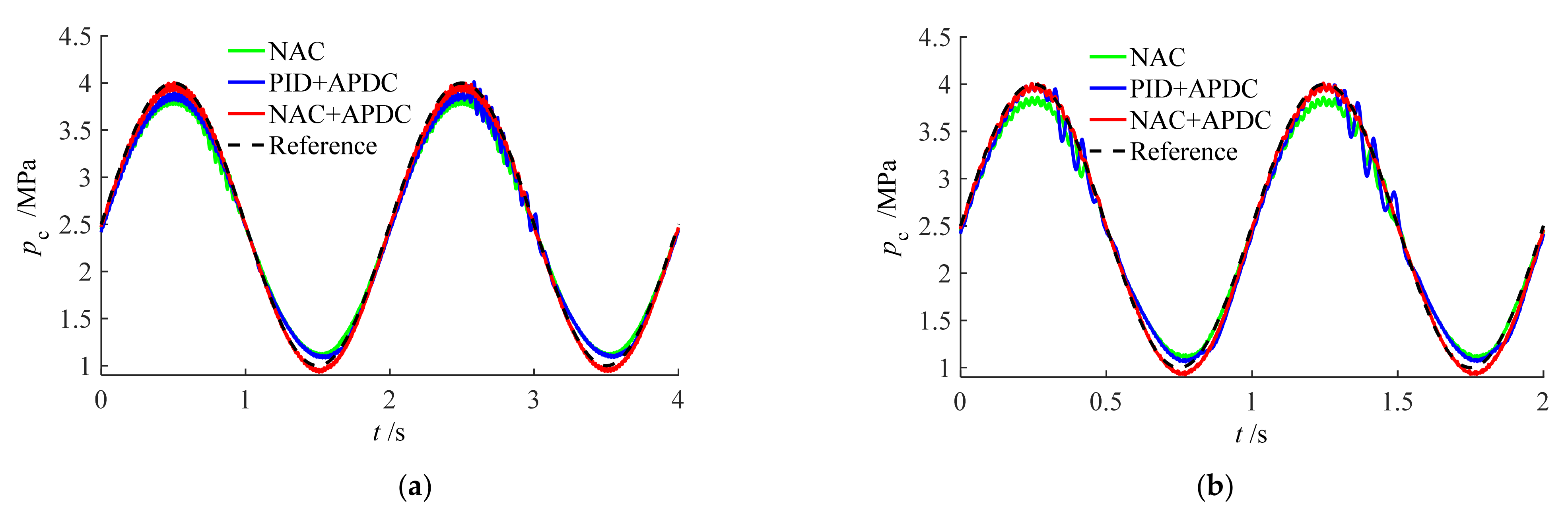
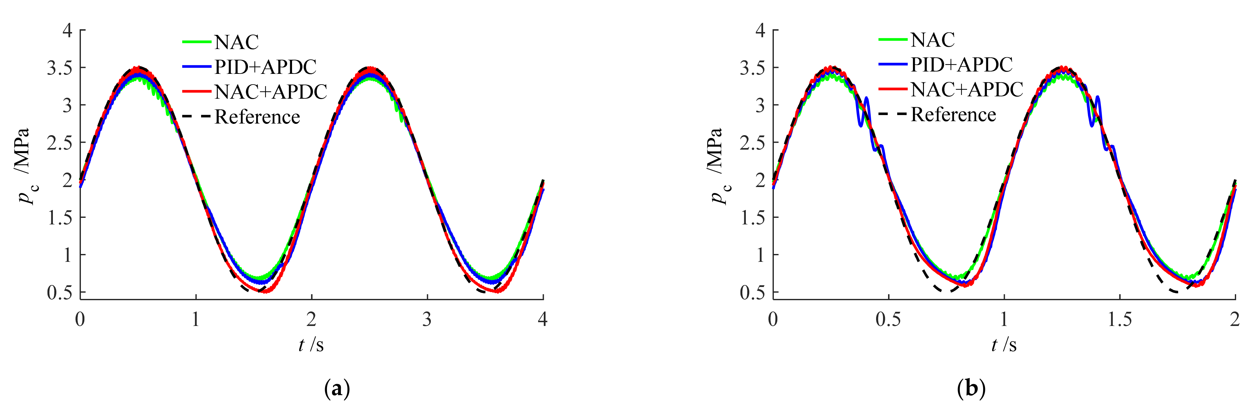
As shown in Figure 15, Figure 16 and Figure 17, when tracking the sinusoidal signal 1.5 sin (2π × 0.5) + 2.5, the NAC + APDC controller has good tracking performance while the tracking errors of the NAC and PID + APDC controllers are large, especially near the peaks and troughs. Moreover, with the increase to the tracking frequency, the responses of the two controllers (NAC and PID + APDC) show a lag. When the offset of the tracking pressure signal was 2 MPa, the NAC and PID + APDC controllers showed bad tracking performance although they maintained the signal shape. Conversely, the NAC + APDC controller still maintained a good tracking performance because the initial duty cycle was always changing when the working pressure changed.
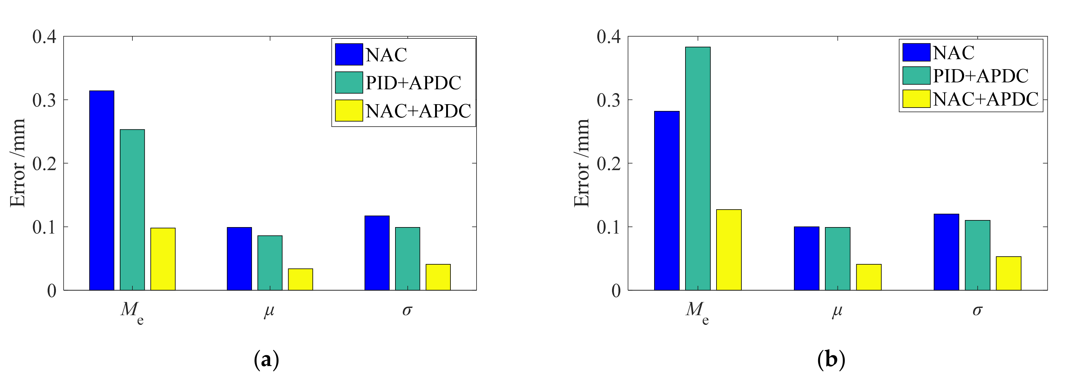
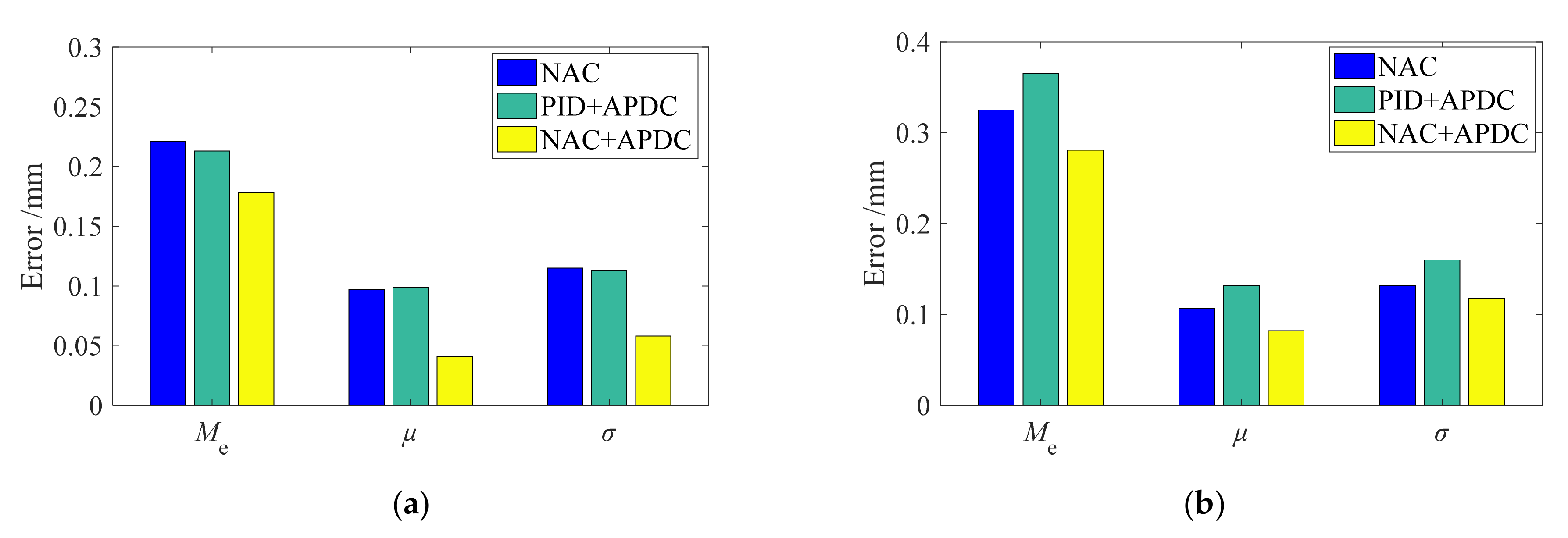
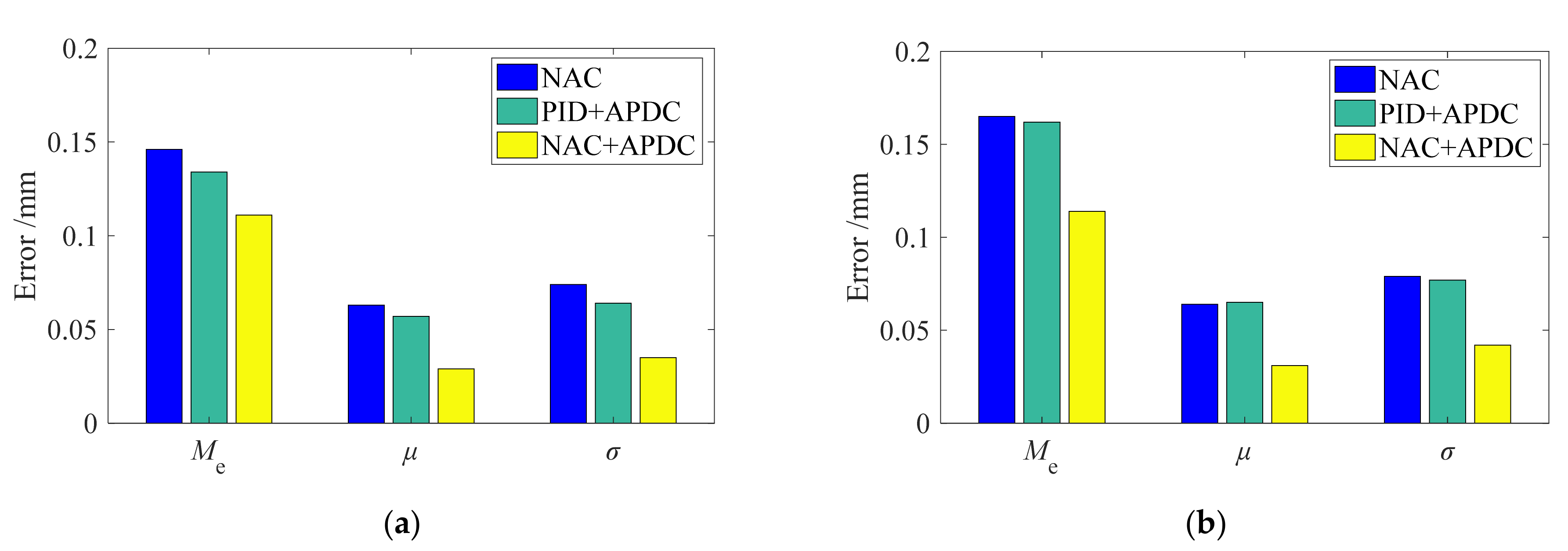
The maximum, average, and standard deviation of the tracking errors (Me, μ, and σ) were used to assess the pressure tracking performance of different controllers [26]. The pressure tracking performance indexes are shown in Figure 18, Figure 19 and Figure 20.
The compared results shown in Figure 18, Figure 19 and Figure 20 indicate that with the proposed NAC + APDC controller, the pressure tracking performances under different amplitudes were good and stable, compared to the NAC controller. For example, when tracking the reference pressure signal 1.5 sin (2π × 0.5) + 2.5, the maximum, average, and standard deviation of the tracking errors of the proposed NAC + APDC were reduced by 68.8%, 65.7% and 65%, compared to the NAC, while the tracking index reductions of the PID + APDC controller were all within 20%.
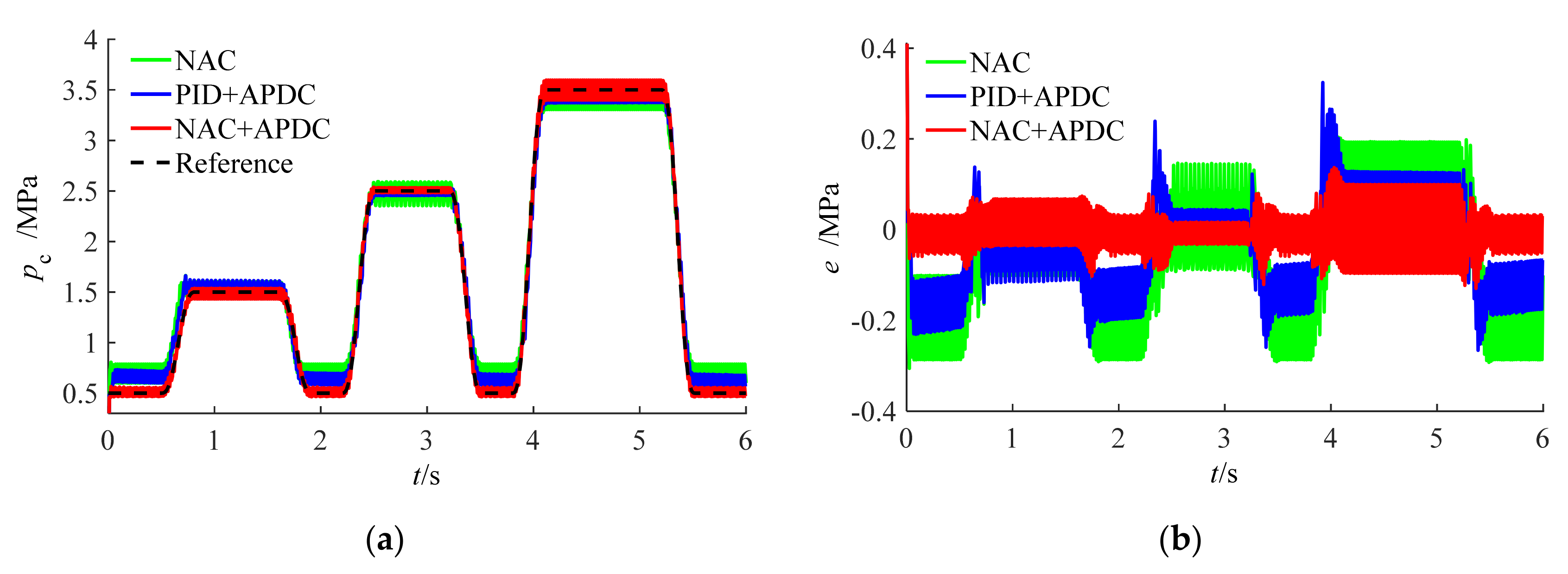
In addition, experimental comparisons of the smooth square pressure signal tracking under the three controllers are shown in Figure 21.
Figure 21 shows that the NAC controller can accurately track the changing pressure but not the fixed pressure, because the pressure difference under different working pressure points was not compensated. Compared to the NAC controller, the tracking performance of the PID + APDC exhibits a little better in fixed pressure but exists a lag in dynamic pressure. Conversely, when using the proposed NAC + APDC controller, the fixed pressure and the dynamic pressure were accurately tracked, although some pressure fluctuations occurred which were acceptable.
6. Conclusions
In this study, a hydraulic pressure servo system based on two high speed on/off valves was designed. The working principles and a mathematical model of the system were presented. A pressure controller consisting of a differential PWM (DPWM) scheme, asymmetric pressure difference compensation (APDC), and nonlinear adaptive control (NAC) was proposed.
- (1)
- The DPWM scheme was designed to improve the resolution of the net flow rate into the testing chamber in which three variables (two initial duty cycles and one control duty cycle) need to be controlled.
- (2)
- The two initial duty cycles of the differential PWM signals were first designed by APDC which can balance the charging ability and the discharging ability under different working pressure points.
- (3)
- The NAC was proposed to calculate the control duty cycle of the DPWM signal which is used to overcome unmodeled dynamic and parameter uncertainties, such as oil compression and leakage.
- (4)
- Extensive comparative experiments demonstrate that, compared to the NAC and PID + APDC controllers, the proposed NAC + APDC controller ensured good tracking performance under different working pressures and tracking frequencies. For example, when tracking pressure signal was 1.5 sin (2π × 0.5) + 2.5, the three tracking indices (maximum error, average error, and error standard deviation) of the proposed NAC + APDC controller were reduced by 68.8%, 65.7% and 65%, respectively, compared to the NAC, while the tracking indexes reduction of the PID + APDC controller were all within 20%.
Funding
This research received no external funding.
Institutional Review Board Statement
Not applicable.
Informed Consent Statement
Not applicable.
Data Availability Statement
Not applicable.
Acknowledgments
This research thanks to experimental help from Nanjing University of Aeronautics and Astronautics.
Conflicts of Interest
The authors declare no conflict of interest.
References
- Nesci, A.; De Martin, A.; Jacazio, G.; Sorli, M. Detection and prognosis of propagating faults in flight control actuators for helicopters. Aerospace 2020, 7, 20. [Google Scholar] [CrossRef] [Green Version]
- Ma, J.G.; Wu, Z.Z.; Guo, H.R.; Li, J. Design and simulation study of a certain landing gear loading simulation system. Adv. Mater. Res. 2014, 871, 69–76. [Google Scholar] [CrossRef]
- Huang, C.; Jiao, Z.X.; Shang, Y.X. Antiskid braking control with on/off valves for aircraft applications. J. Aircr. 2013, 50, 1869–1879. [Google Scholar]
- Lewicki, D.; Stevens, M. Testing of Two-Speed Transmission Configurations for Use in Rotorcraft; NASA/TM-2015–218816; National Aeronautics and Space Administration: Washington, DC, USA, 2015.
- Wu, S.; Zhao, X.Y.; Li, C.F.; Jiao, Z.X.; Qu, Y.F. Multi-objective optimization of a hollow plunger type solenoid for high speed on/off valve. IEEE Trans. Ind. Electron. 2018, 65, 3115–3124. [Google Scholar] [CrossRef]
- Linjama, M.; Laamanen, A.; Vilenius, M. Is it time for digital hydraulics. In Proceedings of the The Eighth Scandinavian International Conference on Fluid Power, Tampere, Finland, 7–9 May 2003. [Google Scholar]
- Gao, Q.; Zhu, Y.; Liu, J. Dynamics modelling and control of a novel fuel metering valve actuated by two binary-coded digital valve arrays. Machines 2022, 10, 55. [Google Scholar] [CrossRef]
- Gao, Q.; Zhu, Y.; Wu, C.; Jiang, Y. Development of a novel two-stage proportional valve with a pilot digital flow distribution. Front. Mech. Eng. 2021, 16, 420–434. [Google Scholar] [CrossRef]
- Van, V.R.B.; Bone, G.M. Accurate position control of a pneumatic actuator using on/off solenoid valves. IEEE/ASME Trans. Mechatron. 1997, 2, 195–204. [Google Scholar]
- Long, G.; Lumkes, J.J. Comparative study of position control with 2-way and 3-way on/off electrohydraulic valves. Int. J. Fluid Power 2010, 11, 21–32. [Google Scholar] [CrossRef]
- Adeli, M.R.; Kakahaji, H. Modeling and position sliding mode control of a hydraulic actuators using on/off valve with PWM technique. In Proceedings of the 3rd International Students Conference on Electrodynamics and Mechatronics, Opole, Poland, 6–8 October 2011; IEEE: New York, NY, USA; pp. 59–64. [Google Scholar]
- Hodgson, S.; Le, M.Q.; Tavakoli, M.; Pham, M.T. Improved tracking and switching performance of an electro-pneumatic positioning system. Mechatronics 2012, 22, 1–12. [Google Scholar] [CrossRef] [Green Version]
- Hodgson, S.; Tavakoli, M.; Pham, M.T.; Tavakoli, M. Nonlinear discontinuous dynamics averaging and PWM-based sliding control of solenoid-valve pneumatic actuators. IEEE/ASME Trans. Mechatron. 2014, 20, 876–888. [Google Scholar] [CrossRef] [Green Version]
- Paloniitty, M.; Linjama, M. High-linear digital hydraulic valve control by an equal coded valve system and novel switching schemes. Proc. IMechE Part I J. Syst. Control Eng. 2018, 232, 258–269. [Google Scholar] [CrossRef]
- Gao, Q.; Linjama, M.; Paloniitty, M.; Zhu, Y.C. Investigation on positioning control strategy and switching optimization of an equal coded digital valve system. Proc. IMechE Part I J. Syst. Control Eng. 2020, 234, 959–972. [Google Scholar] [CrossRef]
- Wang, F.; Gu, L.Y.; Chen, Y. A continuously variable hydraulic pressure converter based on high-speed on-off valves. Mechatronics 2011, 21, 1298–1308. [Google Scholar] [CrossRef]
- Wang, F.; Gu, L.Y.; Chen, Y. A hydraulic pressure-boost system based on high-speed on-off valves. IEEE/ASME Trans. Mechatron. 2013, 18, 733–743. [Google Scholar] [CrossRef]
- Zhao, X.; Li, L.; Song, J.; Li, C.F.; Gao, X. Linear control of switching valve in vehicle hydraulic control unit based on sensorless solenoid position estimation. IEEE Trans. Ind. Electron. 2016, 63, 4073–4085. [Google Scholar] [CrossRef]
- Chen, L.; Wang, H.; Cao, D.P. High-Precision Hydraulic Pressure Control Based on Linear Pressure-Drop Modulation in Valve Critical Equilibrium State. IEEE Trans. Ind. Electron. 2017, 64, 7984–7993. [Google Scholar]
- Jiao, Z.X.; Liu, X.C.; Shang, Y.X.; Huang, C. An integrated self-energized brake system for aircrafts based on a switching valve control. Aerosp. Sci. Technol. 2017, 60, 20–30. [Google Scholar] [CrossRef]
- Lin, Z.L.; Zhang, T.H.; Xie, Q. Intelligent real-time pressure tracking system using a novel hybrid control scheme. Trans. Inst. Meas. Control 2018, 40, 3744–3759. [Google Scholar] [CrossRef]
- Yang, G.; Chen, K.; Du, L.L.; Du, J.M.; Li, B.R. Dynamic vacuum pressure tracking control with high-speed on-off valves. Proc. IMechE Part I J. Syst. Control Eng. 2018, 232, 1325–1336. [Google Scholar] [CrossRef]
- Yang, G.; Jiang, P.; Lei, L.; Wu, Y.; Du, J.M.; Li, B.R. Adaptive backstepping control of vacuum servo system using high-speed on-off valves. IEEE Access 2020, 8, 129799–129812. [Google Scholar] [CrossRef]
- Gao, Q.; Zhu, Y.C.; Luo, Z.; Bruno, N. Investigation on adaptive pulse width modulation control for high speed on off valve. J. Mech. Sci. Technol. 2020, 34, 1711–1722. [Google Scholar] [CrossRef]
- Zhong, Q.; Wang, X.L.; Zhou, H.Z.; Xie, G.; Hong, H.C.; Yan, Y.B.; Chen, B.; Yang, H.Y. Investigation into the adjustable dynamic characteristic of the high-speed on/off valve with an advanced pulsewidth modulation control algorithm. IEEE/ASME Trans. Mechatron. 2021, 1–14. [Google Scholar] [CrossRef]
- Deng, W.X.; Yao, J.Y. Asymptotic tracking control of mechanical servosystems with mismatched uncertainties. IEEE/ASME Trans. Mechatron. 2021, 26, 2204–2214. [Google Scholar] [CrossRef]
Figure 1.
Schematic diagram of a pressure servo system based on two HSVs.

Figure 2.
Relationship between the HSV flow rate and the command signal.

Figure 3.
Adaptive PWM signal and static flow rate of the HSV under adaptive PWM. (a) Adaptive PWM in publication. (b) Static flow rate of the HSV under adaptive PWM.
Figure 3.
Adaptive PWM signal and static flow rate of the HSV under adaptive PWM. (a) Adaptive PWM in publication. (b) Static flow rate of the HSV under adaptive PWM.

Figure 4.
Simulation results of the charging and discharging process under different switching frequencies: (a) 10 Hz; (b) 20 Hz and (c) 50 Hz.
Figure 4.
Simulation results of the charging and discharging process under different switching frequencies: (a) 10 Hz; (b) 20 Hz and (c) 50 Hz.

Figure 5.
Differential PWM control scheme.

Figure 6.
Relationships between the initial duty cycles and the working pressure.

Figure 7.
Diagram of the control algorithm.

Figure 8.
Comparison between the open loop and NAC.

Figure 9.
Simulations of sinusoidal tracking (offset is 2.5 MPa, amplitude is 1.5 MPa) at: (a) 0.5 Hz and (b) 1 Hz.
Figure 9.
Simulations of sinusoidal tracking (offset is 2.5 MPa, amplitude is 1.5 MPa) at: (a) 0.5 Hz and (b) 1 Hz.

Figure 10.
Simulations of sinusoidal tracking (offset is 2 MPa, amplitude is 1.5 MPa) at: (a) 0.5 Hz and (b) 1 Hz.
Figure 10.
Simulations of sinusoidal tracking (offset is 2 MPa, amplitude is 1.5 MPa) at: (a) 0.5 Hz and (b) 1 Hz.

Figure 11.
Simulations of sinusoidal tracking (offset is 2 MPa, amplitude is 1 MPa) at: (a) 0.5 Hz and (b) 1 Hz.
Figure 11.
Simulations of sinusoidal tracking (offset is 2 MPa, amplitude is 1 MPa) at: (a) 0.5 Hz and (b) 1 Hz.

Figure 12.
Simulation results for smooth square tracking: (a) pressure tracking and (b) tracking error.
Figure 12.
Simulation results for smooth square tracking: (a) pressure tracking and (b) tracking error.

Figure 13.
Experimental platform of the pressure servo system.

Figure 14.
Experimental results of the charging and discharging process under different switching frequencies: (a) 10 Hz; (b) 20 Hz and (c) 50 Hz.
Figure 14.
Experimental results of the charging and discharging process under different switching frequencies: (a) 10 Hz; (b) 20 Hz and (c) 50 Hz.

Figure 15.
Experiments of sinusoidal tracking (offset is 2.5 MPa, amplitude is 1.5 MPa) at: (a) 0.5 Hz and (b) 1 Hz.
Figure 15.
Experiments of sinusoidal tracking (offset is 2.5 MPa, amplitude is 1.5 MPa) at: (a) 0.5 Hz and (b) 1 Hz.

Figure 16.
Experiments of sinusoidal tracking (offset is 2 MPa, amplitude is 1.5 MPa): (a) 0.5 Hz and (b) 1 Hz.
Figure 16.
Experiments of sinusoidal tracking (offset is 2 MPa, amplitude is 1.5 MPa): (a) 0.5 Hz and (b) 1 Hz.

Figure 17.
Experiments of sinusoidal tracking (offset is 2 MPa, amplitude is 1 MPa) at: (a) 0.5 Hz and (b) 1 Hz.
Figure 17.
Experiments of sinusoidal tracking (offset is 2 MPa, amplitude is 1 MPa) at: (a) 0.5 Hz and (b) 1 Hz.

Figure 18.
Tracking error of different controllers (offset is 2.5 MPa, amplitude is 1.5 MPa): (a) 0.5 Hz and (b) 1 Hz.
Figure 18.
Tracking error of different controllers (offset is 2.5 MPa, amplitude is 1.5 MPa): (a) 0.5 Hz and (b) 1 Hz.

Figure 19.
Tracking error of different controllers (offset is 2 MPa, amplitude is 1.5 MPa) at: (a) 0.5 Hz and (b) 1 Hz.
Figure 19.
Tracking error of different controllers (offset is 2 MPa, amplitude is 1.5 MPa) at: (a) 0.5 Hz and (b) 1 Hz.

Figure 20.
Tracking error of different controllers (offset is 2 MPa, amplitude is 1 MPa) at: (a) 0.5 Hz and (b) 1 Hz.
Figure 20.
Tracking error of different controllers (offset is 2 MPa, amplitude is 1 MPa) at: (a) 0.5 Hz and (b) 1 Hz.

Figure 21.
Experimental results of the smooth square tracking: (a) pressure tracking and (b) tracking error.
Figure 21.
Experimental results of the smooth square tracking: (a) pressure tracking and (b) tracking error.

Publisher’s Note: MDPI stays neutral with regard to jurisdictional claims in published maps and institutional affiliations. |
© 2022 by the author. Licensee MDPI, Basel, Switzerland. This article is an open access article distributed under the terms and conditions of the Creative Commons Attribution (CC BY) license (https://creativecommons.org/licenses/by/4.0/).
Share and Cite
MDPI and ACS Style
Gao, Q. Nonlinear Adaptive Control with Asymmetric Pressure Difference Compensation of a Hydraulic Pressure Servo System Using Two High Speed On/Off Valves. Machines 2022, 10, 66. https://doi.org/10.3390/machines10010066
AMA Style
Gao Q. Nonlinear Adaptive Control with Asymmetric Pressure Difference Compensation of a Hydraulic Pressure Servo System Using Two High Speed On/Off Valves. Machines. 2022; 10(1):66. https://doi.org/10.3390/machines10010066
Chicago/Turabian StyleGao, Qiang. 2022. "Nonlinear Adaptive Control with Asymmetric Pressure Difference Compensation of a Hydraulic Pressure Servo System Using Two High Speed On/Off Valves" Machines 10, no. 1: 66. https://doi.org/10.3390/machines10010066
Note that from the first issue of 2016, this journal uses article numbers instead of page numbers. See further details here.