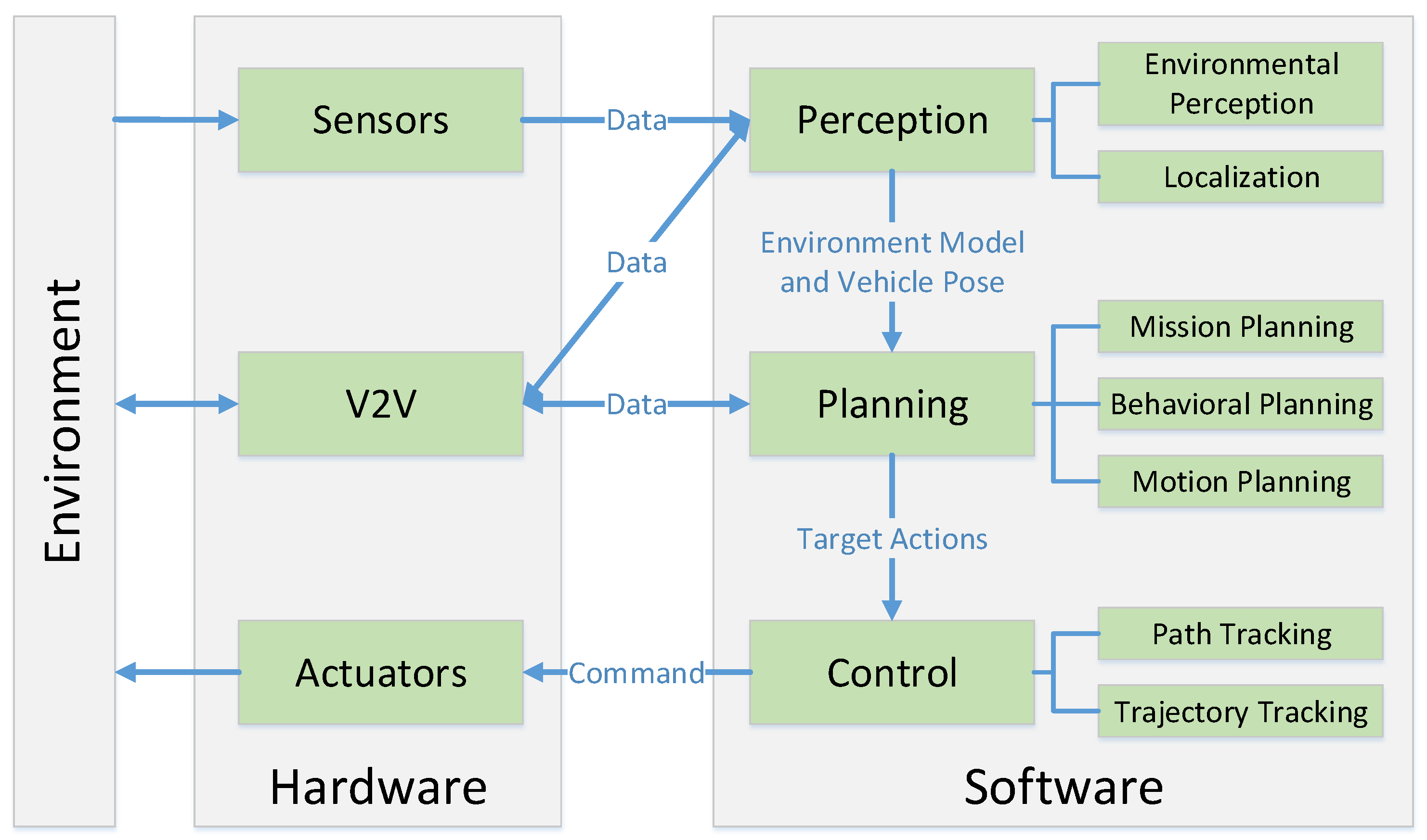
Perception, Planning, Control, and Coordination for Autonomous Vehicles

Abstract

Autonomous vehicles are expected to play a key role in the future of urban transportation systems, as they offer potential for additional safety, increased productivity, greater accessibility, better road efficiency, and positive impact on the environment. Research in autonomous systems has seen dramatic advances in recent years, due to the increases in available computing power and reduced cost in sensing and computing technologies, resulting in maturing technological readiness level of fully autonomous vehicles. The objective of this paper is to provide a general overview of the recent developments in the realm of autonomous vehicle software systems. Fundamental components of autonomous vehicle software are reviewed, and recent developments in each area are discussed.

1. Introduction

Autonomous Vehicles (AVs) are widely anticipated to alleviate road congestion through higher throughput, improve road safety by eliminating human error, and free drivers from the burden of driving, allowing greater productivity and/or time for rest, along with a myriad of other foreseen benefits. The past three decades have seen steadily increasing research efforts in developing self-driving vehicle technology, in part fueled by advances in sensing and computing technologies which have resulted in reduced size and price of necessary hardware. Furthermore, the perceived societal benefits continue to grow in scale along with the rapid global increase of vehicle ownership. As of 2010, the number of vehicles in use in the world was estimated to be 1.015 billion [1], while the world population was estimated to be 6.916 billion [2]. This translates to one vehicle for every seven persons. The societal cost of traffic crashes in the United States was approximately 300 billion USD in 2009 [3]. The financial cost of congestion is continually increasing each year, with the cost estimate for United States reaching as high as 160 billion USD in 2014 [4]. The associated health cost of congestions in United States was estimated to be over 20 billion USD in 2010 from premature deaths resulting from pollution inhalation [5]. While it is uncertain just how much these ongoing costs can be reduced through autonomous vehicle deployment, attempting to curtail the massive scale of these numbers serves as great motivation for the research.

A future with self-driving cars was first envisioned as early as 1918 [6], with the idea even broadcasted over television as early as 1958 [7]. By 1988, Carnegie Mellon’s NAVLAB vehicle was being demonstrated to perform lane-following using camera images [8]. Development was accelerated when several research teams later developed more advanced driverless vehicles to traverse desert terrain in the 2004 and 2005 DARPA Grand Challenges [9], and then urban roads in the 2007 DARPA Urban Challenge (DUC) [10]. Research related to self-driving has since continued at a fast pace in academic settings, but furthermore is now receiving considerable attention in industry as well.

As research in the field of autonomous vehicles has matured, a wide variety of impressive demonstrations have been made on full-scale vehicle platforms. Recent studies have also been conducted to model and anticipate the social impact of implementing autonomous Mobility-on- Demand (MoD) [11]. The case studies have shown that MoD system would make access to mobility more affordable and convenient compared to traditional mobility system characterized by extensive private vehicle ownership.

Autonomous driving on urban roads has seen tremendous progress in recent years, with several commercial entities pushing the bounds alongside academia. Google has perhaps the most experience in the area, having tested its fleet of autonomous vehicles for more than 2 million miles, with expectation to soon launch a pilot MoD service project using 100 self-driving vehicles [12]. Tesla is early to market their work, having already provided an autopilot feature in their 2016 Model S cars [13]. Uber’s mobility service has grown to upset the taxi markets in numerous cities worldwide, and has furthermore recently indicated plans to eventually replace all their human driven fleet with self-driving cars [14], with their first self-driving vehicle pilot program already underway [15].

There are several places where automated road shuttles are in commercial operations. Examples include deployments at Rivium Business Park, Masdar City, and Heathrow Airport [16,17]. The common feature of these operations is that road vehicles are certified as a rail system meaning that vehicles operate in a segregated space [17]. This approach has been necessary due to legal uncertainty around liability in the event of an accident involving an autonomous vehicle. To address this, governments around the world are reviewing and implementing new laws. Part of this process has involved extended public trials of automated shuttles, with CityMobil and CityMobil2 being among the largest of such projects [17].

While the majority of the research contributions discussed in the remaining sections of this article are from academic institutions, it is worth noting that the industrial market interest is also largely responsible for research investigations into certification and validations processes, especially in regards to autonomous car manufacturability and services [18,19]. These topics are however left out of the scope of this survey paper.

Driving in urban environments has been of great interest to researchers due in part to the high density of vehicles and various area-specific traffic rules that must be obeyed. The DARPA Urban Challenge [20], and more recently the V-Charge Project [21] catalyzed the launch of research efforts into autonomous driving on urban road for numerous organizations. Referring to Figure 1, the problem of urban driving is both interesting and difficult because it pushes the research direction to address both increased operating speeds of autonomous vehicles as well increased environmental complexity.

The core competencies of an autonomous vehicle software system can be broadly categorized into three categories, namely perception, planning, and control, with the interactions between these competencies and the vehicle’s interactions with the environment depicted in Figure 2. Also, Vehicle-to-Vehicle (V2V) communications can be leveraged to achieve further improvements in areas of perception and/or planning through vehicle cooperation.

Perception refers to the ability of an autonomous system to collect information and extract relevant knowledge from the environment. Environmental perception refers to developing a contextual understanding of environment, such as where obstacles are located, detection of road signs/marking, and categorizing data by their semantic meaning. Localization refers to the ability of the robot to determine its position with respect to the environment.

Planning refers to the process of making purposeful decisions in order to achieve the robot’s higher order goals, typically to bring the vehicle from a start location to a goal location while avoiding obstacles and optimizing over designed heuristics.

Finally, the control competency, refers to the robot’s ability to execute the planned actions that have been generated by the higher level processes.

The main objective of this paper is to provide a general overview of the recent developments in the realms of autonomous vehicle software system. However, as there has been a massive surge in research interest in the field of autonomous system in recent years, this paper is by no means a complete survey of the currently available hardware and software systems in the literature. The remainder of this paper is organized as follows: In Section 2, the topics of environmental perception and localization are discussed. Section 2.1 focuses on recent advances in LIDAR (Light Detection and Ranging) and camera based signal processing techniques in particular. Section 2.2 reviews the methods of localizing the vehicle with respect to its environment, especially with map-based localization techniques. Autonomous vehicle decision making processes are reviewed in Section 3, with greater emphasis in the areas of behavioral and motion planning. Section 4 discusses the theoretical design and practical implementation of autonomous vehicle control systems. Recent advances in the field of multi-vehicle cooperation will be reviewed in Section 5, and finally Section 6 concludes the paper.

2. Perception

2.1. Environmental Perception

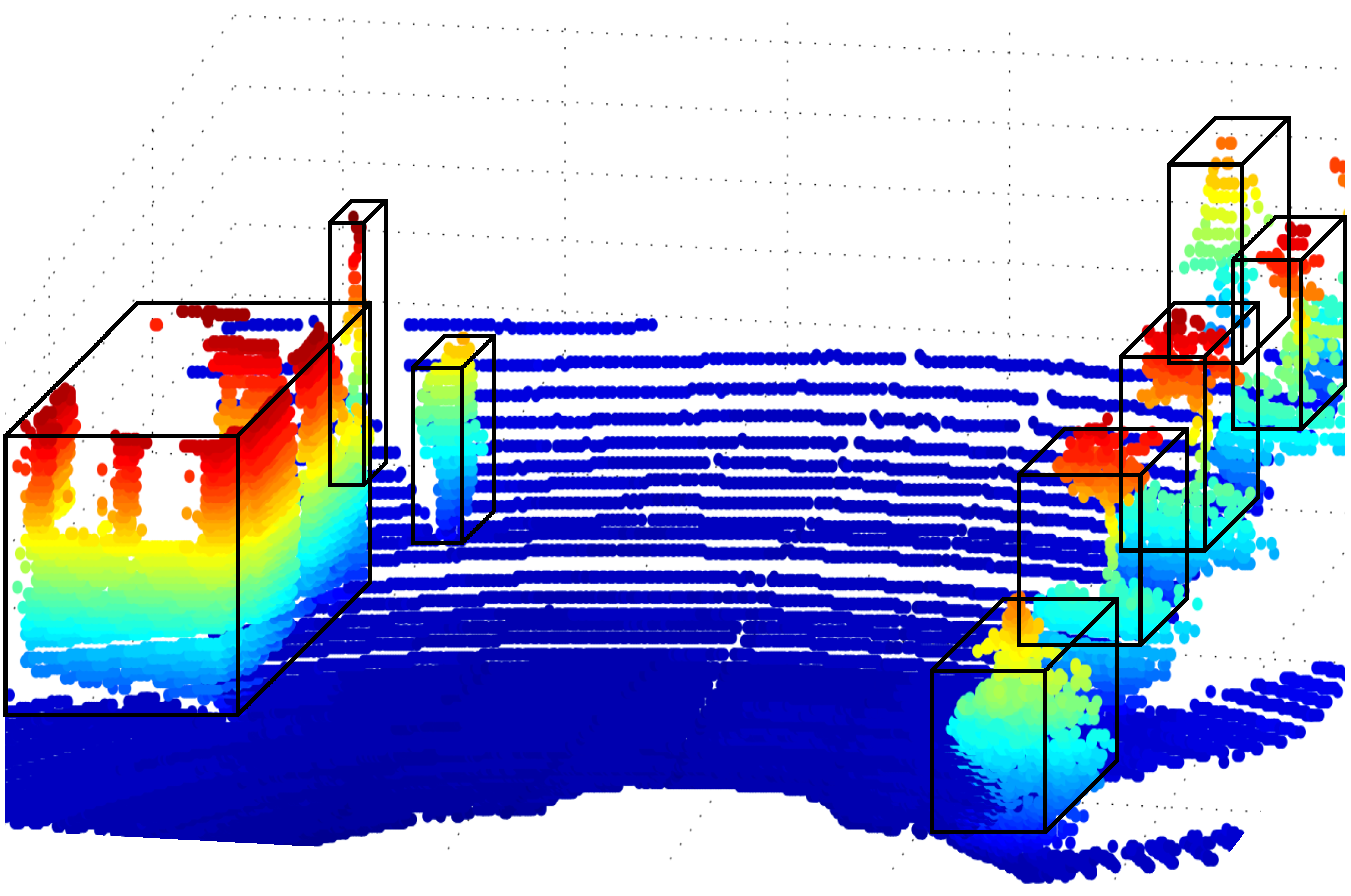
Environment perception is a fundamental function to enable autonomous vehicles, which provides the vehicle with crucial information on the driving environment, including the free drivable areas and surrounding obstacles’ locations, velocities, and even predictions of their future states. Based on the sensors implemented, the environment perception task can be tackled by using LIDARs, cameras, or a fusion between these two kinds of devices. Some other traditional approaches may also involve the use of short/long-range radars and ultrasonic sensors, which will not be covered in this paper. Regardless of the sensors being implemented, two critical elements of the perception task are (i) road surface extraction and (ii) on-road object detection.

2.1.1. LIDAR

LIDAR refers to a light detection and ranging device, which sends millions of light pulses per second in a well-designed pattern. With its rotating axis, it is able to create a dynamic, three-dimensional map of the environment. LIDAR is the heart for object detection for most of the existing autonomous vehicles. Figure 3 shows the ideal detection results from a 3D LIDAR, with all the moving objects being identified.

In a real scene, the points returned by the LIDAR are never perfect. The difficulties in handling LIDAR points lie in scan point sparsity, missing points, and unorganized patterns. The surrounding environment also adds more challenges to the perception as the surfaces may be arbitrary and erratic. Sometimes it is even difficult for human beings to perceive useful information from a visualization of the scan points.

Representation

The output from the LIDAR is the sparse 3D points reflected back from the objects, with each point representing an object’s surface location in 3D with respect to the LIDAR. Three main representations of the points are commonly used, including point clouds, features, and grids [23].

Point cloud based approaches directly use the raw sensor data for further processing. This approach provides a finer representation of the environment, but at the expense of increased processing time and reduced memory efficiency. To mitigate this, usually a voxel-based filtering mechanism is applied to the raw point cloud to reduce the number of points, e.g., [24,25].

Feature based approaches first extract parametric features out of the point cloud and represent the environment using the extracted features. The features that are commonly used include lines [26] and surfaces [27]. This approach is the most memory-efficient, but it is often too abstract, and its accuracy is subject to the nature of the point cloud, as not all environment features can be approximated well by aforementioned set of feature types.

Grid based approaches discretize the space into small grids, each of which is filled with information from the point cloud such that a point neighborhood is established [28]. As pointed out in [23], this approach is memory-efficient and has no dependency on predefined features. However, it is not straightforward to determine the size of the discretization. In [29], an adaptive octree was created to guide the segmentation from coarse grids to fine ones.

Segmentation Algorithms

To perceive the 3D point cloud information, normally two steps are involved: segmentation and classification. Some may include a third step, time integration, to improve the accuracy and consistency. Segmentation of point cloud is the process of clustering points into multiple homogeneous groups, while classification is to identify the class of the segmented clusters, e.g., bike, car, pedestrian, road surface, etc.

As summarized in the survey paper [30], the algorithms for 3D point cloud segmentation can be divided into five categorizes: edge based, region based, attributes based, model based, and graph based. In this section, we will provide supplementary reviews to reveal the recent development in this field. As a result, a new category is identified, which is based on deep learning algorithms.

Edge based methods are mainly used for particular tasks in which the object must have strong artificial edge features, like road curb detection [31,32]. However, it is not a useful approach for nature scene detection and is susceptible to noise. To improve the robustness, in [33], the elevation gradients of principal points are computed, and a gradient filter is applied to filter out points with fluctuations.

Region based methods make use of region growing mechanisms to cluster neighborhood points based on certain criteria, e.g., Euclidean distance [34,35] or surface normals [36]. In most cases, the process starts with generating some seed points and then growing regions from those points according to a predefined criteria. As compared against the edge based method, this approach is more general and practical. It also avoids the local view problem as it takes neighborhood information into account. In [37], a scan-line based algorithm was proposed to identify the local lowest points, and those points were taken as the seeds to grow into ground segments based on slope and elevation. A feature based on the normal vector and flatness of a point neighborhood was developed in [38] to grow the regions in trees and non-planar areas. To make the growing process more robust, a self-adaptive Euclidean clustering algorithm was proposed in [34]. In [39], a new attribute “unevenness,” which was derived based on the difference between the ranges of successive scanning rings from each laser beam, was proposed as the growing criteria. As claimed in [40,41,42], it was more capable of detecting small obstacles and less sensitive to the presence of ground slopes, vehicle pitch, and roll.

In the literature, some researchers also looked into how to effectively generate the seed points by taking more heuristics into account so that they can lead to a more effective and robust region growing process. In [43], Vieira et al. first removed points at sharp edges based on curvatures before selecting the seed points, since good seed points are typically found in the interior of a region, rather than at its boundaries. In [44], the normal of each point was first estimated, then the point with the minimum residual was selected as the initial seed point, while in [45], the local plane, instead of normal, at each point was extracted and a corresponding score was computed followed by the selection of seed planes based on the score. A multi-stage seed generation process was proposed in [28]. Non-empty voxels were grouped into segments based on proximity, and these segments served as the seeds for the next segmentation process, which made use of the coherence and proximity of the coplanar points. Finally the neighborhood coplanar point segments are merged based on plane connection and intersection.

The region based segmentation methods have been implemented widely in the literature, however as pointed out in [29,30,46,47], the segmentation results depend too heavily on the selection of the seed points. Poorly selected points may result in inadequate and inefficient segmentations, and different choices of seed points usually lead to different segmentations [25]. Additionally, all of the region based methods require extensive computation resources, taxing both time and memory [29,48].

Model based methods, also known as parametric methods, first fit the points into predefined models. These models, like plane, sphere, cone, and cylinder, normally can be expressed effectively and compactly in a closed mathematic form. Those inliers to a particular model are clustered as one segment. Most of the model based methods are designed to segment the ground plane. The two most widely implemented model fitting algorithms in the literature are RANSAC (Random Sample Consensus) and HT (Hough Transform). Therefore, the model based methods share the same pros and cons as these two algorithms.

In [24,27,32,49,50], the authors implemented the RANSAC algorithm to segment the ground plane in the point cloud with the assumption of flat surface. However, as mentioned in [23,51], for non-planar surfaces, such as undulated roads, uphill, downhill, and humps, this model fitting method is not adequate.

To mitigate these defects, Oniga et al. [52] fitted the plane into quadratic form instead of planar form based on RANSAC. Then a region growing process was designed to refine the quadratic plane. Asvadi et al. in [51] divided the space in front of the vehicle into several equal-distant (5 m) strips and fit one plane for each strip based on least square fitting. In [23], a piecewise ground surface estimation was proposed, which consist of four steps: slicing, gating, plane fitting, and validation. The slicing step slices the space in front of the vehicle into regions with approximately equal number of LIDAR points, whereas the gating step rejects outliers in each region based on interquartile range method. RANSAC plane fitting is then applied to each sliced region to find all the piecewise planes, and a final validation step is carried out by examining the normal and height differences between consecutive planes.

The HT model fitting methods can also be found in the literature to fit different models, e.g., planes, cylinders, and spheres. In [53,54], the 3D HT was applied on point level and normal vectors to identify planar structures in the point clouds, whereas in [55], the authors proposed a sequential HT algorithm to detect cylinders in the point cloud. This sequential approach reduced the time and space complexity as compared to the conventional approach which required 5-D Hough space.

As elaborated above, the model based methods are well established in the literature for planar surface extraction. Normally, these methods are used as a primary step in segmentation to remove the ground plane, while other methods, e.g., region growing, are then applied to cluster the remaining points. However, the major disadvantage of model based methods is that it does not take neighborhood and context information into account, and thus it may force random points into a particular model. Furthermore, the segmentation is sensitive to the point cloud density, position accuracy, and noise [29].

Attribute methods normally take a two-step approach, where the first step is to compute the attribute for each point, and the second step is to cluster the points based on the associated attributes. As mentioned in [30], this set of methods allow for more cues to be incorporated into the formulation on top spatial information. However, the success of the segmentation also depends strongly on the derived hidden attributes.

Besides those works reviewed in [30], the attribute based algorithm proposed in [56] demonstrated that it was capable of segmenting pole-like objects, which was considered as challenging due to its thin feature. In this algorithm, the optimal neighborhood size of each point was first calculated. The geometric features, taking the neighboring information into account, were derived based on PCA (Principle Component Analysis). Each point was then assigned with three types of attributes (linear, planar, and spherical) using LIBSVM [57] by taking the geometric features as input. Finally, segmentation rules were designed to cluster the points based on their associated attributes.

The other group of methods that are widely used in the literature is graph based methods. These methods cast the point cloud into a graph structures with each point as the vertex/node and the connection between neighbor points as graph edges. The graph based method has demonstrated its strength in image semantic segmentation as it is able to incorporate local and global cues, neighborhood information, context, smoothness, and other customized features into its formulation and optimize the segmentation globally across the entire image.

Following the graph cut methods in image segmentation, in the content of point cloud, they always follow the form of CRF (Conditional Random Field [58]) or MRF (Markov Random Field), and the optimization is normally through min-max flow cut algorithm or its variations.

In [59,60], the authors first created a k-nearest neighbors graph, assigned each node according to a background penalty function, added hard foreground constraints, and solved the foreground and background segmentation through min-cut. Moosmann et al. [25] used the graph based method to segment ground and objects using a unified and generic criterion based on local convexity measures.

As to be shown later, the graph based methods have also been implemented as the pipelines for sensor fusion between LIDAR and vision. Compared to other methods, graph based ones are more robust in dealing with complex scene due to their global features as aforementioned. The major issue with these methods is that it normally takes more time to compute, especially for the optimization part.

With the recent development in machine learning algorithms in computer vision, some researchers also looked into how to apply machine learning architectures, which are normally applied to 2D image, into the 3D point cloud for segmentation and detection. A commonly used dataset is proposed in [61], which contains a colored 3D point cloud of several Haussmanian style facades.

In [62], the author implemented the Random Forest classifier to classify each point into one semantic class. The classifier was trained based on the light-weight 3D features. Afterwards, individual facades were separated by detecting differences in the semantic structure. To improve the memory efficiency and segmentation accuracy, Riegler et al. [63] proposed an Octree Network based on 3D convolution. It exploits the sparsity in the point cloud and focuses memory allocation and computation in order to enable a deeper network without compromising resolution.

This set of algorithms is recently developed and thus has some crucial and practical issues which makes it difficult to achieve real time operation. However, they do provide new insights into the point cloud segmentation problem. As to be shown in the detection algorithm, they can provide a unified pipeline to combine the segmentation and detection processes.

Detection Algorithm

After the segmentation, each cluster needs to be categorized into different objects. The information embedded in each cluster is mainly from spatial relationship and the LIDAR intensity of the points, which has very limited use in object recognition. Thus most of the algorithms will leverage the detection problem on computer vision through some fusion mechanisms as to be shown later. However, there does exist some other research works exploring the possibility to perform object recognition from point cloud data.

In [25], the authors proposed a primary classifier to recognize ground clusters. For each segment, a histogram over all the surface normal vectors’ height values was generated, and if the last bin contained the most votes, that segment was classified as ground. This algorithm is not able to differentiate the objects above the ground.

Zhang et al. [64] proposed an SVM (Support Vector Machine) based classifier to classify the clusters into ground, vegetation, building, power line, and vehicle. In total 13 features were derived as the input to the SVM classifier. However, this classifier is still very coarse, which is not practical enough for the autonomous vehicle applications.

The recently developed machine learning algorithms are more general and robust as compared to the aforementioned ones as they are able to recognize more categories of objects. In [65], VoxNet was proposed, which implemented a 3D convolutional neural network to classify the 3D point cloud (in occupancy grid/volumetric representation). While in [66], the volumetric based 3D CNN was improved by introducing auxiliary learning tasks on part of an object and combining data augmentation with multi-orientation pooling. In [67], a 3D Convolutional Deep Belief Network was proposed to learn the distribution of complex 3D shapes across different object categories and arbitrary poses from raw CAD data.

However, as mentioned in [63], for 3D networks, the computational and memory requirements increase cubically with the input size of the 3D point cloud. All the aforementioned methods can only operate at the order of ${30}^3$ voxels, which is able to fully exploit the rich and detailed geometry of 3D objects. As reviewed in the segmentation part, the Octree Networks in [63] is a more efficient architecture to handle the 3D point cloud. It has improved the input cluster resolution from the order of ${30}^3$ to ${256}^3$.

2.1.2. Vision

The vision system in autonomous vehicle environment perception normally involves road detection and on-road object detection. The road detection also includes two categories: lane line marking detection and road surface detection. In the following sections, we will review the works under each of the categories. At the same time, the recently developed deep learning approaches will be included. For more information on conventional hand-crafted feature/cue based approaches, interested readers may refer to the following survey papers: [68,69] for lane line marking detection, [70] for road surface detection, [71,72] for vehicle detection and [73] for pedestrian detection.

Lane Line Marking Detection

Lane line marking detection is to identify the lane line markings on the road and estimate the vehicle pose with respect to the detected lines. This piece of information can be served as the vehicle position feedback to vehicle control systems. A vast amount of research work has been done in this domain since a few decades ago [8]. However, it is yet to be completely solved and has remained as a challenging problem due to the wide range of uncertainties in real traffic road conditions and road singularities [74], which may include shadows from cars and trees, variation of lighting conditions, worn-out lane markings, and other markings such as directional arrows, warning text, and zebra crossings [75].

As summarized in the survey paper by Hillel et al. in [68], most of the lane line detection algorithms share three common steps: (1) lane line feature extraction, by edge detection [76,77] and color [78,79], by learning algorithms such as SVM [80], or by boost classification [81,82]; (2) fitting the pixels into different models, e.g., straight lines [83,84], parabolas [85,86], hyperbolas [87,88,89], and even zigzag line [90]; (3) estimating the vehicle pose based on the fitted model. A fourth time integration step may exist before the vehicle pose estimation in order to impose temporal continuity, where the detection result in the current frame is used to guide the next search through filter mechanisms, such as Kalman filter [76,91] and particle filter [80,90,92].

Lane line feature extraction is to identify the pixels that belong to lane line markings and eliminate non-lane line marking pixels. Most approaches in the literature are based on the observations that lane markings have large contrast compared to road pavement.

Some gradient based algorithms can be commonly found in the literature, e.g., Sobel edge detector with symmetrical local threshold [93], adaptive thresholding [91], and gradient-enhancing conversion [94]. However, these algorithms are sensitive to noise and can result in a large number of outliers from clutter and shadows. Furthermore, they are limited to local view and ignore the shape feature of lane line markings (long and thin bright structures).

Some other more advanced variants based on image gradient have been proposed in the literature, which are less sensitive to noise. For example, the steerable filter ([69,85]) is based on second order derivatives of 2D Gaussians, and ridge detector ([95,96]) is based on tensor field construction of first order derivatives. Both methods are able to obtain the response of gradient directions which facilitates to remove outliers if their directions deviate too much from the presumed lane line direction.

Another set of algorithms attempts to detect lane line markings from a different perspective, searching for low-high-low intensity pattern along image rows. The most common algorithm of this type is the box filter (also known as the top-hat filter) or other forms of variants, e.g., [97,98,99,100]. They are considered as more reliable than the aforementioned algorithms. In brief, they convolute the image with a certain form of step filter and select the high response pixels as the lane line candidates at each image row. Normally, they are capable of extracting the medial axis of lane line markings instead of edges.

For this kind of algorithm to work properly, its scale or step width must be tuned accurately according to the lane line marking width in the image, to prevent under/over filtering. Otherwise, the original image has to be transformed through inverse-perspective mapping (IPM) to compensate for the camera perspective effect (e.g., [101,102]). However, this also requires a good estimation of camera pitch angle (or viewing angle). At the same time, interpolation is needed to make up for the missing pixels in the IPM image. As the viewing distance becomes larger, the interpolation becomes more and more inaccurate. To solve this problem, Du et al. [90] provide an adaptive mechanism to update the step width online based on the previous width measurements.

Another shortcoming that is common to the aforementioned lane line extraction algorithms is that they cannot distinguish lane line markings from other on-road markings, such as warning letters, humps and so on. These on-road markings may occasionally result in severe estimation errors.

The second step is model fitting. It is the process to extract a compact high-level representation of the lane from the lane line detection results. Depending on the model used, the vehicle pose can be derived from the fitted model as shown in [88,95]. The model can also be used to guide the lane line detection in the next frame to improve continuity (e.g., [90,103,104]).

Various road models have been proposed in the literature. Those reviewed above are parametric models. Another category is semi-parametric, which mainly consists of splines, such as B-Snake [105], Cubic splines [80], active contours [106], etc. The advantage of these models is that they are more flexible and can cover various road shapes. However, they are more computationally demanding and complex. They also require a good selection of control points. As concluded in [68], since there is no single model that can cover all kinds of road shapes, online model selection should be considered.

The time integration step is to make use of previous information to guide the search in the current image. It imposes smoothness and continuity between consecutive images. It can improve vehicle pose estimation accuracy and prevent erroneous detection failures.

Most of the proposed approaches are stochastic. For example, the Kalman filter can be found in [69,97,107], and particle filter is applied in [80,85,92,104]. As pointed out in [68], the particle filter is more reliable, especially under abrupt changes in between consecutive images induced by vehicle vibrations or non-flat road surfaces.

In general, the particle filter can be implemented directly to the image (or pixels), lane line model, and vehicle. For example, in [80], each particle contains the locations of control points in the image for cubic spline fitting. In [92,102], each particle represents lane line model parameters. The change of parameters is simply assumed to follow a Gaussian distribution. However, they did not mention how the covariance matrix was obtained. In [85], each particle represents the location of the vehicle in real world coordinates, but again the motion of vehicle is simply assumed to be Gaussian. Since the change between consecutive images is purely due to the vehicle motion, Du et al. [90] provided a more intuitive and straightforward approach which applied the particle filter to the moving vehicle and took its explicit dynamic model into account.

The last step in the lane-level localization is to estimate the vehicle lateral position and moving orientation based on the lane line model. To recover this information from 2D image to 3D real world, depth is required. In most approaches, depth is derived from the camera viewing angle or pitch angle by assuming constant camera height and flat road surface. One typical example is the IPM, but it depends strongly on the pitch angle and it is sensitive to pitch angle estimation noise.

A more reliable and direct way to recover the depth is through stereo cameras, given that the disparity image can be constructed effectively and accurately. However, as mentioned in [68], the low texture of road surface poses a processing challenge to obtain the disparity image. This is the main reason why stereo is not widely adopted in this research field. In [108], the author used dense mapping to obtain disparity while in [109], Maximum A Posteriori - Markov Random Field (MAP-MRF) approach was applied. However, both methods are not very effective and subject to smoothing noise. To mitigate these drawbacks, Du et al. [90] proposed a lane line model based correspondence matching algorithm.

Road Surface Detection

Road surface detection informs the autonomous vehicle on the locations of free space where it can drive without collision. It is the prerequisite for any online path planning and control operations. Generally speaking, the approaches can be divided into three categories: feature/cue based detection, feature/cue based learning, and deep learning.

The feature/cue based detection approaches first identify the feature points or patches in the original image based on some predefined features (e.g., HOG). In the context of stereo images, the feature may refer to the disparity. Based on the identified features, either model fitting or segmentation kind of algorithms will be applied to identify the road surfaces.

In [110], a general B-spline model fitting algorithm was applied based on the stereo disparity measurement to represent the road surface. This approach dropped the assumption of flat road surface. And a Kalman filter was designed to further smooth the fitting results.

Instead of using model fitting, [111] cast the road surface detection problem into a CRF optimization problem. The authors constructed the CRF energy function by taking both object class labeling and dense stereo reconstruction into the formulation and jointly optimized these two tasks, which improved the performance of each individual task.

The feature/cue learning based approaches also extract a set of features associated to pixels or image patches and then train a classifier based on the features to assign a road or non-road label to the pixels or patches.

In [112], the authors proposed a detection algorithm to learn the contextual information which can facilitate the classification of the targeted image patch. For each image patch, besides itself, it is also associated with another two types of auxiliary image patches: the contextual patches obtained based on a predefined pattern surrounding the target image patch and road patches positioned at the bottom part of the image. Three feature vectors are extracted from these three types of patches and then concatenated into one single final vector. The vector is fed to a MLP (Multilayer Perceptron) neural network to do classification. However, this method is not able to take the global information into account and the selection of the road patches is controversial, as it is based on the assumption that the bottom part of the image is always road region.

Tobias et al. [113] proposed a two-hierarchy detection framework which incorporated the spatial layout of the scene to handle a high variety of complex situations. The first layer consists of three base classifiers for road boundary, road and lane markings. The three classifiers are trained separately to generate three confidence maps. The spatial ray features that incorporate properties of the global environment are generated based on the confidence maps. Finally, a GentleBoost classifier [114] was trained based on the spatial ray features.

In both [115,116], the classifier, which used a joint boosting algorithm, incorporated the feature maps based on textons (filter-bank, color, HoG and location) and disptons (U-disptons and V-disptons).

However, all these aforementioned algorithms under feature detection or feature learning categories are not robust enough under the erratic driving environments. The performances are still subjected to all the noise factors as listed in the lane line marking detection section.

As shown in the well-know database KITTI [117], the top five performances for road detection (excluding those non-published entries) all fall under the category of deep learning. As highlighted in [70], the deep learning framework has gained popularity during the past few years, especially with the development of suitable processors and implementations [118].

Both [119,120] took an image patch as the input to the Convolutional Neural Network (CNN) which classified the center point of the image patch as to whether it was road or not. In [120], the author also demonstrated how to incorporate the spatial information of the patch into the CNN to enable the learning of spatial priors on top of appearances.

Different from these two approaches, Mohan [121] proposed a novel architecture that integrated the CNN with deep de-convolutional neural networks. The architecture was also employed for multi-patch training, which made it possible to effectively learn spatial priors from scenes. This approach has yielded the state-of-the-art performance in the KITTI dataset.

Despite its excellent performance, the drawbacks of deep learning approaches are also very obvious: huge computation and memory requirement, long process time, non-traceable, and tedious ground truth annotation process. In [122], a new CNN structure was proposed with the aim to achieve a good trade-off between segmentation quality and runtime. This also integrated a CNN with deep de-convolution network, but a new mapping between classes and filters at the de-convolution side was designed to reduce the runtime. It took the entire image at its original resolution, instead of image patches, as network input and achieved a run time of about 50 ms.

To mitigate the difficulties in ground truth annotation, Laddha et al. [123] proposed map-supervised deep learning pipeline. In this approach, the ground truth annotation was done automatically based on the vehicle position, heading direction, camera parameters, GPS, and OpenStreetMap data. The annotation noise was further reduced by using pixel appearance features. A CNN was trained based on these machine generated ground truth annotations.

On-Road Object Detection

On-road object detection mainly concerns vehicle and pedestrian object classes. Due to the various types, appearances, shapes, and sizes of the objects, those methods reviewed in [71,72,73] are not robust and not general enough for the application of autonomous vehicles. As listed in the KITTI database, for car, pedestrian, and cyclist detections, all of the leading entries and state of the art methods are based on deep learning schemes. Deep learning has shown its superior performance as compared to conventional learning or feature based approaches in the domain of obstacle detection. Therefore, in this section, we will only review the deep learning based approaches.

Normally, the general pipeline for deep learning approaches is that a set of proposal bounding boxes needs to be generated around the input image, then each proposal box will be sent through the CNN network to determine a classification (including background) and fine tune its bounding box locations as well. The common methods for bounding box proposal are Selective Search [124] and EdgeBoxes [125], which both rely on inexpensive hand-crafted features and economical inference schemes.

In [126], an energy minimization approach was presented for bounding box proposal. These proposals were generated by exhaustively placing 3D bounding boxes on the ground-plane, projecting them to the image plane and scoring them via simple and efficiently computable image features including semantic and object instance segmentation, context, shape features, and location priors to score the boxes. Per-class weights were also learnt for these features using S-SVM, adapting to each individual object class.

Faster-RCNN [127] was the first deep learning scheme that unify both the bounding box proposal and detection under the same network and achieved an end-to-end training process. The network consists of two major parts: proposal net and detection net, where these two nets share most of the CNN layers. The output from the proposal net are the proposed bounding boxes, which is used as the input to the detection net for recognition and bounding box fine tuning processes.

Although in the training process Faster-RCNN does not fix the proposal box sizes and thus is supposed to be invariant to object scales, but when it comes to challenging scenarios where the scales of the object vary dramatically, its performance on small object detection is not very satisfying. The main reason is that for small objects in the original image, after several layers of convolution and pooling, the remaining information in the last layer is too little for a good detection. This issue can be addressed by enlarging the input image size or by using a set of images at different scale sizes as input [128], but this will increase the computation time and memory requirement as well.

To address the scale issue, in [129], Yang et al. proposed a scale-dependent pooling (SDP) network. Instead of pooling the feature vectors only from the last convolution layer in the network, the feature vectors for smaller proposal bounding boxes were pooled in earlier convolution layers according to box heights. The detection and bounding box fine tuning were carried out separately at different layers accordingly. To improve the efficiency, the author also trained a classical cascaded rejection classifiers (CRC) based on MLP to filter out some proposal boxes at every layer. This approach is not unified and not able to be trained end-to-end. The bounding box proposal was based on Edgebox.

In [130], the authors proposed a unified multi-scale deep learning network (MS-CNN), which took the original image as the only input and output the bounding boxes and object categories for the associated bounding boxes. Similar to Faster-RCNN, this network also combined a proposal net and detection net. Similar to the SDP net, the proposal net in MS-CNN pooled features from different layers to generate bounding box proposals. All these proposals were then passed to the same detection net for object recognition and bounding box fine tuning.

All the aforementioned algorithms target to detect the object in the 2D image, with no output information on the 3D world. In [131], by further dividing the object category into sub-categories based on their 2D appearance, 3D pose and 3D shape, the authors were able to train the deep learning network to recover both 2D and 3D information from the 2D image. The proposed network, named as Sub-CNN, consisted of two CNN networks, subcategory-aware CNN and object detection CNN. The subcategory-aware CNN generated proposal bounding boxes to the object detection network. Unlike Faster-RCNN and MS-CNN, these two networks did not share any CNN layers. In the KITTI benchmark, both MS-CNN and Sub-CNN achieved similar state-of-the-art performance in object detection. Sub-CNN took longer run time (2 s vs. 0.4 s) since it had two separated CNN nets, but it was able to reveal the 3D world information which is more useful for autonomous vehicles.

There also exists some other approaches in the literature to reduce the processing time so that the deep learning approach can achieve (near) real time performance, e.g., YOLO (You Only Look Once) [132], SSD (Single Shot Detection) [133]. They are able to process the images at more than 30 frames per second, varying with the size of the network. However, the fast performance is achieved at the expense of detection rate. As the technologies in both hardware and software develop further, a better trade-off between the run time and detection rate can be achieved.

2.1.3. Fusion

Different sensors have different strengths and weaknesses. Sensor fusion techniques are required to make full use of the advantages of each sensor. In the context of autonomous vehicle environment perception, LIDAR is able to produce 3D measurements and is not affected by the illumination of the environment, but it offers little information on objects’ appearances; conversely, camera is able to provide rich appearance data with much more details on the objects, but its performance is not consistent across different illumination conditions; furthermore, camera does not implicitly provide 3D information.

Following [134], the techniques that have been applied to LIDAR and camera fusion can be roughly divided into two main categories based on their fusion process locations, including fusion at feature level (early stage, centralized fusion) and fusion at decision level (late stage, decentralized fusion). Based on the fusion mechanisms, they can be divided into the following categories: MRF/CRF based, probability based, and deep learning based.

In [135], each point in the point cloud has an associated pixel in the image, based on the transform between the LIDAR device and camera. Thus the color intensity of the pixel can be assigned to the point. An MRF was designed by converting the point cloud into a graph with all of the points being graph nodes. The energy minimization function modelled the correlations between the changes in intensity and depth of the points. This approach only made use of the intensity information from image and ignored the rest of the image cues.

Xiao et al. also proposed a random field approach in [136] for sensor fusion but with different energy formulation as compared to [135]. The energy function consists of three terms, out of which, two were the same as normal MRF terms (value term and smoothness term). The third term was based on the laser points. A classifier was pre-trained to classify the laser points as to whether they were road or non-road points. These points were then projected to the image plane, and the corresponding pixels were assigned with the same probability of the points. The third term was derived from these probabilities.

In [137], instead of using sparse laser points directly, the author reconstructed the dense depth map from the point cloud by upsampling the points. Two sets of HOG (histogram of gradient) pyramids based on the original image and the dense depth map were extracted, and a multi scale deformable part model [138] was learnt for pedestrian detection based on the HOG pyramids.

Premebida et al. [139] provided a decentralized approach for sensor fusion. The camera data was used to train an AdaBoost classifier while the LIDAR data was used to train a GMM (Gaussian Mixture Model) classifier [140]. A sum decision rule, based on the posteriori probabilities calculated by each classifier was then designed to ultimately classify an object.

The deep learning based sensor fusion scheme always requires a dense depth map or its variants, indicating that the point cloud needs to be converted into depth map. For example, in [141], the image and the depth map went through two separated CNN networks, and only the feature vectors from the last layer were concatenated to jointly carry out the final detection task. In [142], the point cloud was first converted into a three-channel HHA map (which contains Horizontal disparity, Height above ground, and Angle). The HHA and RGB (Red-Green-Blue color channel) images went through two different CNN networks as well but the author found that the fusion should be done at the early to middle layers of the CNN instead of the last layer.

In conclusion, sensor fusion between LIDAR and camera is necessary in order to make the best use of these devices and achieve a robust environment perception result for autonomous vehicles. However, the current fusion mechanisms are still in a preliminary stage and not able to fully make use of all the information from both sensors. Furthermore, those newly developed deep learning algorithms for object detection, as reviewed in Section 2.1.2, have not yet been extended to operate over fused camera and LIDAR information, where such an extension could yield significant performance boosts over individual sensor data processing.

2.2. Localization

Localization is the problem of determining the pose of the ego vehicle and measuring its own motion. It is one of the fundamental capabilities that enables autonomous driving. However, it is often difficult and impractical to determine the exact pose (position and orientation) of the vehicle, and therefore the localization problem is often formulated as a pose estimation problem [143].

The problem of estimating the ego vehicle’s pose can generally be divided into two sub-problems, namely the pose fixing problem and the dead reckoning problem. In the pose fixing problem, the measurement is related to the pose by an algebraic/transcendental equation. Pose fixing requires the capacity to predict a measurement given a pose, e.g., a map. In the dead reckoning problem, the state is related to the observation by a set of differential equations, and these equations have to be integrated in order to navigate. In this case, sensor measurements may not necessarily be inferable from a given pose. In this sense, pose fixing and dead reckoning complement each other.

One of the most popular ways of localizing a vehicle is the fusion of satellite-based navigation systems and inertial navigation systems. Satellite navigation systems, such as GPS and GLONASS, can provide a regular fix on the global position of the vehicle. Their accuracy can vary from a few of tens of meters to a few millimetres depending on the signal strength, and the quality of the equipment used. Inertial navigation systems, which use accelerometer, gyroscope, and signal processing techniques to estimate the attitude of the vehicle, do not require external infrastructure. However, without the addition of other sensors, the initiation of inertial navigation system can be difficult, and the error grows in unbounded fashion over time.

The use of GPS in localization requires reliable service signals from external satellites. This method is reliable only when the GPS signal and dead reckoning odometry of the vehicle is reliable, and may require expensive, high-precision sensors. A few good examples of problematic areas are in indoor environments, underground tunnels, and urban canyons, where tall buildings deny good GPS signal readings to the vehicle. In [144,145], road matching algorithms which use a prior road map to constrain the motion of the vehicle are used in conjunction with GPS and INS to update the localization estimation of the vehicle. The inclusion of road matching improves the accuracy in global localization. However, the method still couldn’t fully achieve precise pose estimation of the vehicle with respect to its environment to the level required for autonomous driving.

Map aided localization algorithms use local features to achieve highly precise localization, and have seen tremendous development in recent years. In particular, Simultaneous Localization and Mapping (SLAM) has received much attention. The goal of SLAM is to build a map and use it concurrently as it is built. SLAM algorithms leverage old features that have been observed by the robot’s sensors to estimate its position in the map and locate new features. Although it is not possible to determine the absolute position, SLAM uses statistical modelling that takes into account the odometry of the vehicle to remove most of the inconsistency between where the features are predicted to be and where it is based on the sensor readings. In general there are two approaches to SLAM problem: Bayesian filtering and smoothing.

The goal of formulating SLAM as a Bayesian filtering problem is to estimate the joint posterior probability $p(x_{1:t},m|z_{1:t},u_{1:t-1})$ about the map m and robot trajectory $x_{1:t}=x_1,\cdots ,x_t$, given its sensor measurement $z_{1:t}=z_1,\cdots ,z_t$, and inputs to the system $u_{1:t-1}=u_1,\cdots ,u_{t-1}$. Popular methods in this category are Extended Kalman Filter (EKF), Extended Information Filter (EIF), and Particle Filter (PF) [146,147,148,149].

A variation of the Particle Filter, Rao-Blackwellized Particle Filters(RBPF), has also been introduced as a solution to the SLAM problem in [150,151]. In RBPF, the vehicle’s trajectory and the associated map are represented by a particle, and factorizes the probabilities according to the following equation:

$$p(x_{1:t},m|z_{1:t},u_{1:t-1})=p\left(m\right|x_{1:t},z_{1:t})·p\left(x_{1:t}\right|z_{1:t},u_{1:t-1})$$

(1)

This equation is referred to as Rao-Blackwellization, and allows the trajectory of the vehicle to be first computed before the map is constructed based on the computed trajectory. This approach provides efficient computation since the map is strongly correlated to the vehicle’s trajectory. The posterior probability $p\left(x_{1:t}\right|z_{1:t},u_{1:t-1})$ is computed with a particle filter, in which the prior distribution is obtained from the vehicle’s odometry, and refined with observations/sensor readings.

Pose graph mapping [152] is a popular example of smoothing based SLAM. The SLAM problem is formulated as an optimization problem to minimize the error, by exploiting the inherent sparsity of a map. A few recently proposed algorithms of this type are TreeMap [153], TORO [154], iSAM [155], iSAM2 [156], and g2o [157].

A key event in smoothing based SLAM is the loop closure, which happens when features that have not been seen for a while are observed again from the sensor readings. When a loop closure is detected, the error caused by imperfect odometry can then be removed, and a substantial portion of the map can be updated. The simplest way of doing loop closure is by performing pair wise matching for possible loop closure by considering all observations that are within a pre-determined radius from a node in the pose graph [158]. More elaborate ways of detecting loop closures are also available in the literature, such as by learning from range sensor data [159], or probabilistically from visual appearance [160].

Rejecting false loop closure constraints is still an open research problem. Robust automatic loop closure detection is still a very active research topic. Various extension to the current SLAM algorithm to make the loop closure detection more robust such as Switchable Constraint method [161], Max-Mixture Model [162], and Realizing, Reversing, Recovering techniques [163] have been proposed in recent literature.

Scan matching is another key event in pose graph construction. Popular algorithms include Iterative Closest Point (ICP) [164], where each reference scan is matched with a query scan by aligning them according to a distance metric [165], and feature histogram based scan matching algorithms, such as Normal Distribution Transform (NDT) [166] and Spin Images [167].

Embedding the map with additional information is another active research topic. The term semantic mapping is widely referred to in the literature as augmenting the traditional metric/topological map with a higher level semantic understanding of the environment. In general, approaches to semantic mapping can be categorized into three categories: object based, appearance based, and activity based.

Appearance based semantic mapping techniques interpret sensor readings to construct semantic information of the environment. A few examples, such as [168,169], use geometric features from planar LIDARS. Vision can also be fused with LIDAR data for further classification and understanding of the environment [170,171,172].

Object based semantic mapping uses the occurrence of key objects to build a semantic understanding of the environments [173,174], where object recognition and classification is often a very important event in object based semantic understanding of the environment.

The activity based approach to semantic mapping relies on information about the activities of the agents around the robot. This topic is relatively less mature compared to appearance and object based semantic mapping. A few examples of this technique are found in [174,175] where external agent activities are used to semantically understand and classify the context of the environment (e.g., sidewalk versus road, etc.).

The map-aided localization algorithms can then use these features to localize the robot to a pre-recorded map and based on its surrounding features. In [176], lane markers are extracted from the reflectivity values of LIDAR data and are used as local features. With this approach, instead of using a self learned map, prior knowledge from open source maps such as Open-Street Map can be used, eliminating the map building stage [177]. Virtual 2D ranging is then extracted from 3D point clouds and matched with the map [178]; coupled with GPS and INS data, the position of the vehicle can be estimated with Bayesian filtering methods.

Feature based localization is also another active research topic. The most popular method is by using particle filter to localize the vehicle in real time with 3D LIDARs [179]. The algorithm first analyses the laser range data by extracting points from the road surface. Then, the reflectivity measurements of these points are correlated to a map containing ground reflectivity to update particle weights. One underlying assumption in this algorithm is that the road surface remains relatively constant, which may undermine the performance in some cases.

However, the cost of 3D LIDARs can be prohibitive to many applications. Synthetic methods can be used to obtain 3D measurements from 2D sensors. For example, accumulated laser sweeps can be used as local features. This type of algorithm first generates a swathe of laser data by accumulating 2D laser scans from a tilted-down LIDAR [180], then the swathe is matched to a prior 3D data reference by minimizing an objective function. This algorithm demonstrates its accuracy and robustness in GPS-denied areas. Although an accurate 3D model of the environment in not required, an accurate and consistent prior is always desired when the localization is integrated with other navigation functions. Similarly in [181,182], a 3D point cloud of the environment is obtained by servoing a 2D LIDAR, and extracted 2D features are used to perform localization. This method has been shown to work well in an indoor environment with well structured ceiling features.

3. Planning

3.1. Autonomous Vehicle Planning Systems

Early-stage self-driving vehicles (SDVs) were generally only semi-autonomous in nature, since their designed functionality was typically limited to performing lane following, adaptive cruise control, and some other basic functions [183]. Broader capabilities were notably demonstrated in the 2007 DARPA Urban Challenge (DUC) [184], where it was shown that a more comprehensive planning framework could enable a SDV to handle a wide range of urban driving scenarios. Performance of the SDVs was still far from matching the quality of human drivers and only six of the 35 competition entrants were able to complete the final event, but nevertheless, this milestone demonstrated the feasibility of self-driving in an urban environment [10,42,185,186,187,188] and revealed important research challenges residing in autonomous driving [189].

Boss, the winning entry of the DUC, Junior, the second place entry, and Odin, the third place entry, along with many others, employed similar three level hierarchical planning frameworks with a mission planner, behavioral planner, and motion planner. While the fourth place entry Talos reportedly used a two level planner with a navigator and a motion planner, the navigator essentially performed the functions of both the mission planner and behavioral planner [190]. The mission planner (or route planner) considers high level objectives, such as assignment of pickup/dropoff tasks and which roads should be taken to achieve the tasks. The behavioral planner (or decision maker) makes ad hoc decisions to properly interact with other agents and follow rules restrictions, and thereby generates local objectives, e.g., change lanes, overtake, or proceed through an intersection. The motion planner (or local planning) generates appropriate paths and/or sets of actions to achieve local objectives, with the most typical objective being to reach a goal region while avoiding obstacle collision. Many recent works since the DUC continue to inherit the same three level hierarchical structure as described here, though the partitioning of the layers are somewhat blurred with variations of the scheme occurring in literature.

3.2. Mission Planning

Mission planning generally is performed through graph search over a directed graph network which reflects road/path network connectivity. In the DUC, a Route Network Definition File (RNDF) was provided as prior information [191]. The RNDF represented traversable road segments by a graph of nodes and edges, and further included information such as stop sign locations, lane widths, and parking spot locations. The RNDF was generated manually by the competition organizers, however ongoing research targets to generate richer network representations stored in a Road Network Graph (RNG) through automated processes, via sensing the infrastructure (i.e., road boundaries) directly [192], or even by inference from vehicle motions [193]. Regardless of whether the RNG is generated through manual annotation or through an automated method, the route searching problem is formulated by assigning edge weights corresponding to the cost of traversing a road segment (commonly distance) and applying graph search algorithms. Classical algorithms such as Dijkstra’s [194] or A* [195] can be effective for smaller neighborhoods, however more advanced methods exist to improve efficiency over large networks, which are detailed in a survey paper focused more specifically on the topic of route planning [196].

3.3. Behavioral Planning

The behavioral planner is responsible for decision making to ensure the vehicle follows any stipulated road rules and interacts with other agents in a conventional, safe manner while making incremental progress along the mission planner’s prescribed route. This may be realized through a combination of local goal setting, virtual obstacle placement, adjustment of drivable region bounds, and/or regional heuristic cost adjustment. Decisions were made onboard most DUC vehicles through Finite State Machines (FSMs) of varying complexity to dictate actions in response to specific perceived driving contexts [42,185,187,197]. The terms precedence observer and clearance observer were coined to categorize functions which checked certain logical conditions required for state transitions, where precedence observers were to check whether the rules pertaining to the vehicle’s current location would allow for it to progress, and clearance observers would check “time to collision”—the shortest time by which a detected obstacle would enter a designated region of interest—to ensure safe clearance to other traffic participants. For example, when approaching a stop sign, the SDV would have to both ensure precedence by coming to a complete stop at the stop line and wait for any other stationary vehicles at the intersection with priority to move off, and ensure clearance by measuring time to collision along its intended path (where oncoming traffic may not have to stop at the intersection).

Finite state machines of this nature are limited in that they are manually designed for a set number of specific situations. The vehicle may then perform unexpectedly in a situation that was not explicitly accounted for in the FSM structure, perhaps finding itself in a livelock, or even a deadlock state if there aren’t sufficient deadlock protections. Recent research works have sought to improve organization in large decision making structures to thus manage larger rules sets [198,199,200]. Other works have sought provable assurances in the decision making structure to guarantee adherence to rules sets [201]. In [202,203], road rules enforcement was checked using Linear-Temporal Logic (LTL) considerations, with successful real-world overtaking experiments [203].

3.4. Motion Planning

Motion planning is a very broad field of research, applied to mobile robots and manipulating arms for a wide variety of applications ranging from manufacturing, medical, emergency response, security/surveillance, agriculture and transportation. In the context of mobile robotics, motion planning refers to the process of deciding on a sequence of actions to reach a specified goal, typically while avoiding collisions with obstacles. Motion planners are commonly compared and evaluated based on their computational efficiency and completeness. Computational efficiency refers to the process run time and how this scales based on the dimensionality of the configuration space. The algorithm is considered complete if it terminates in finite time, always returns a solution when one exists, and indicates that no solution exists otherwise [204].

The motion planning problem has been proven to exhibit great computational complexity, especially in high dimensions. For example, the well known piano mover’s planning problem has been shown to be PSPACE-hard [205]. Furthermore, to guarantee completeness may demand an exhaustive search of all possible paths, which leaves many approaches stuck with the “curse of dimensionality” in high dimensional configuration spaces; it is increasingly more difficult to represent all obstacle occupied spaces and check for obstacle free points as the dimension of the search space increases. A core idea behind motion planning is then to overcome this challenge by transforming the continuous space model into a discrete model [206]. Two general categories of approaches to this transformation exist: (1) combinatorial planning, which builds a discrete representation that exactly represents the original problem; and (2) sampling-based planning which utilizes a collision checking module to conduct discrete searching over samples drawn from the configuration space [206]. (A problem is said to belong to PSPACE complexity class if it can be solved by a deterministic Turing machine using an amount of memory (space) that follows the asymptotic trend of $O\left(n^k\right)$, $k\ge 0$, for an input of length n as $n\to \infty$. A deterministic Turing machine is a hypothetical device which operates to change symbols/values on a tape, where each symbol may only be changed one at a time, and only one action is prescribed at a time for any given situation. A problem A is furthermore considered PSPACE-hard if every problem/language B in PSPACE is polynomial-time reducible to A, $B{\le }_{p}A$, meaning any B can be translated into instances of A in polynomial time.)

3.4.1. Combinatorial Planning

Combinatorial planners aim to find a complete solution by building a discrete representation which exactly represents the original problem, but which is characterized by convenient properties for special case solvers. For example, geometric solutions may efficiently be generated in low dimensional spaces with discrete convex obstacle spaces by constructing visibility graphs (shortest path solution), Voronoi-diagrams (highest clearance solution), or decomposing the space into obstacle free “cells” using obstacle boundaries as cell borders [206]. However the computational burden of these methods increases with increased dimensionality of the configuration space and increased number of obstacles, and thus combinatorial methods are typically limited in application. This is the primary motivation for the development of sampling-based algorithms, which will be discussed in the following subsection [207,208,209].

While decomposing spaces directly from obstacle geometry may be difficult in practice, other decompositions became popular where checks would still need to be made against the presence of obstacles. A common simple approach is to apply a uniform discretization over either the configuration search space or set of robot actions such that a finite search may be applied to find solution paths. By working in discretized spaces, the complexity of an exhaustive search is greatly reduced. Although completeness can no longer be guaranteed by these means, these methods may be found to be resolution-complete. That is to say that if the space is discretized to a “fine enough” resolution, then completeness can be guaranteed. Fine resolutions may however still be hard to achieve in high dimensional spaces, leading to excessive computational burden, again from the curse of dimensionality.

Nevertheless, it is still common to employ discretized search methods for road navigation. In the DARPA Grand Challenges and the DUC, many teams implemented a simple motion planner by which a kinodynamic reachable trajectory set was discretized [10], and/or a trajectory search tree was generated based on road geometry [9,10,42]. Such methods are still being refined, with emphasis on optimization of smooth velocity profiles [210]. Cell decomposition over the configuration space has also been used with some success [185]. An optimal path would typically be found over the finite discretization by implementing graph search algorithms, such as A* [195].

Recent works have also made use of space discretization in order to apply more advanced decision making algorithms. For example, cell decomposition was used in [201,211] to then generate paths which would obey road rules specified via Linear Temporal Logic (LTL). Tumova et al. [212] used similar LTL methods to further investigate situations where the robot was allowed to break some rules (such as always drive in your lane) in order to reach goals that were otherwise obstructed. Cell decomposition was also necessary to apply popular models for handling environment uncertainty, such as Partially Observable Markov Decision Processes (POMDP) and Mixed Observability Markov Decision Processes (MOMDP). In [213,214], other moving obstacles’ intentions were inferred in real-time while the robot’s motion plan was executed concurrently. POMDPs assume uncertainty in both the robot’s motion and in observation and account for this uncertainty in solving for optimal policies, where MOMDPs have extended this idea to situations in which some of the state variables are partially observable and others are full observable [215]. It’s worth noting that POMDPs have been gaining popularity recently with the emergence of efficient point based value iteration solvers like SARSOP [216]. Prior to the emergence of SARSOP and other popular approximation algorithms, POMDPs were often avoided in robotics because solving POMDPs exactly is computationally intractable and the framework scales poorly with increasing number of states and increasing planning horizon [217]. Recent research has also targeted means to apply POMDP to continuous spaces [218].

3.4.2. Sampling-Based Planning

Sampling-based methods rely on random sampling of continuous spaces, and the generation of a feasible trajectory graph (also referred to as a tree or roadmap) where feasibility is verified through collision checking of nodes and edges to connect these nodes. Roadmaps generated should ideally provide good coverage and connectivity of all obstacle-free spaces. Paths over the roadmap are then used to construct solutions to the original motion planning problem. Sampling-based algorithms are popular for their guarantees of probabilistic completeness, that is to say that given sufficient time to check an infinite number of samples, the probability that a solution will be found if it exists converges to one. While sampling-based algorithms are generally applied over continuous spaces, it should be noted that some discretization typically occurs in collision checking, especially along edge connections in the roadmap.

Variants of sampling-based algorithms primarily differ in the method by which a search tree is generated. Probabilistic RoadMaps (PRM) [209,219] and Rapidly-exploring Random Trees (RRT) [220,221] are perhaps two of the most influential sampling-based algorithms, each of which have been popular subjects of robotics research with many variants suggested. PRM is a multi-query method which builds and maintains multiple graphs simultaneously, and has been shown particularly effective in planning in high-dimension spaces [219]. RRT in contrast seeks to rapidly expand a single graph, which is suitable for many mobile robotics applications where the map is not well known a priori due to the presence of dynamic obstacles and limited sensor coverage concentrated around the robot’s current location.

In many applications, besides completeness guarantees and efficiency in finding a solution, the quality of the returned solutions is also important. While an initial solution might be found quickly in many cases, the algorithms are typically run for a longer period of time to allow for better solutions to be found based on some heuristics. Some works have proposed to bias tree growth toward regions that resulted in lower cost solutions [222]. Many sampling-based planners and variants of PRM and RRT have since been proposed. A comprehensive evaluation of many popular planners was presented in [207], where many popular planners were not only compared on a basis of computational complexity and completeness, but also on optimality. The authors showed that the popular PRM and RRT algorithms are actually asymptotically sub-optimal, and proposed asymptotically optimal variants, PRM* and RRT*. Other asymptotically optimal planners have since been suggested, such as Fast Marching Trees (FMT*) [223] and Stable Sparse Trees (SST*) [224], both of which claim speed improvement over RRT*.

3.5. Planning in Dynamic Environments

Many operating environments are not static, and are therefore not known a priori. In an urban environment, the traffic moves, road detours and closures occur for construction or accident cleanup, and views are frequently obstructed. The robot must constantly perceive new changes in the environment and be able to react while accounting for several uncertainties. Uncertainties arise from perception sensor accuracy, localization accuracy, environment changes, and control policy execution [225,226,227,228,229,230,231,232]. However, in application, perhaps the largest source of uncertainty is the uncertainty in surrounding obstacles’ movements.

3.5.1. Decision Making Structures for Obstacle Avoidance

An approach taken by many DARPA Urban Challenge vehicles was to monitor regions along the intended path for potential obstacle collisions, where these regions would be labeled as “critical zones” [42], or merge zones at intersection, and checked against the trajectories of all nearby vehicles to determine a “time to collision”. Typically, if a collision was seen as imminent, the vehicle would slow or stop accordingly, which was acceptable behavior for crossing and merging at many intersections [190], though perhaps overly conservative in other situations. In [233], the lane ahead was checked for presence of a vehicle traveling in the wrong direction on a collision path, where if triggered, a “defensive driving” maneuver would be executed to pull off the lane to the right side and stop. When defensive driving behavior was tested in other vehicles, the performance was unsatisfactory in that the oncoming vehicle had to stop before the autonomous vehicle would move to navigate around it [188]. The approaches had an advantage of computational simplicity in that they planned in a low dimensional space neglecting the time dimension, but the resulting behaviors were overly simplistic in that a deterministic set behavior was executed without heuristic weighting of alternative actions or explicit consideration for environment evolution given the chosen course of action. Nevertheless, recent works have still continued to use behavioral level decision making for obstacle avoidance, especially to handle difficult maneuvers such as lane changing [198].

Other stochastic decision making structures, such as Partially Observable Markov Decision Processes (POMDP), can explicitly model uncertainties in vehicle controls and obstacle movements and have been applied with success in some complex scenarios [213], but these methods can be difficult to generalize and required discretization of the state space and vehicle controls.

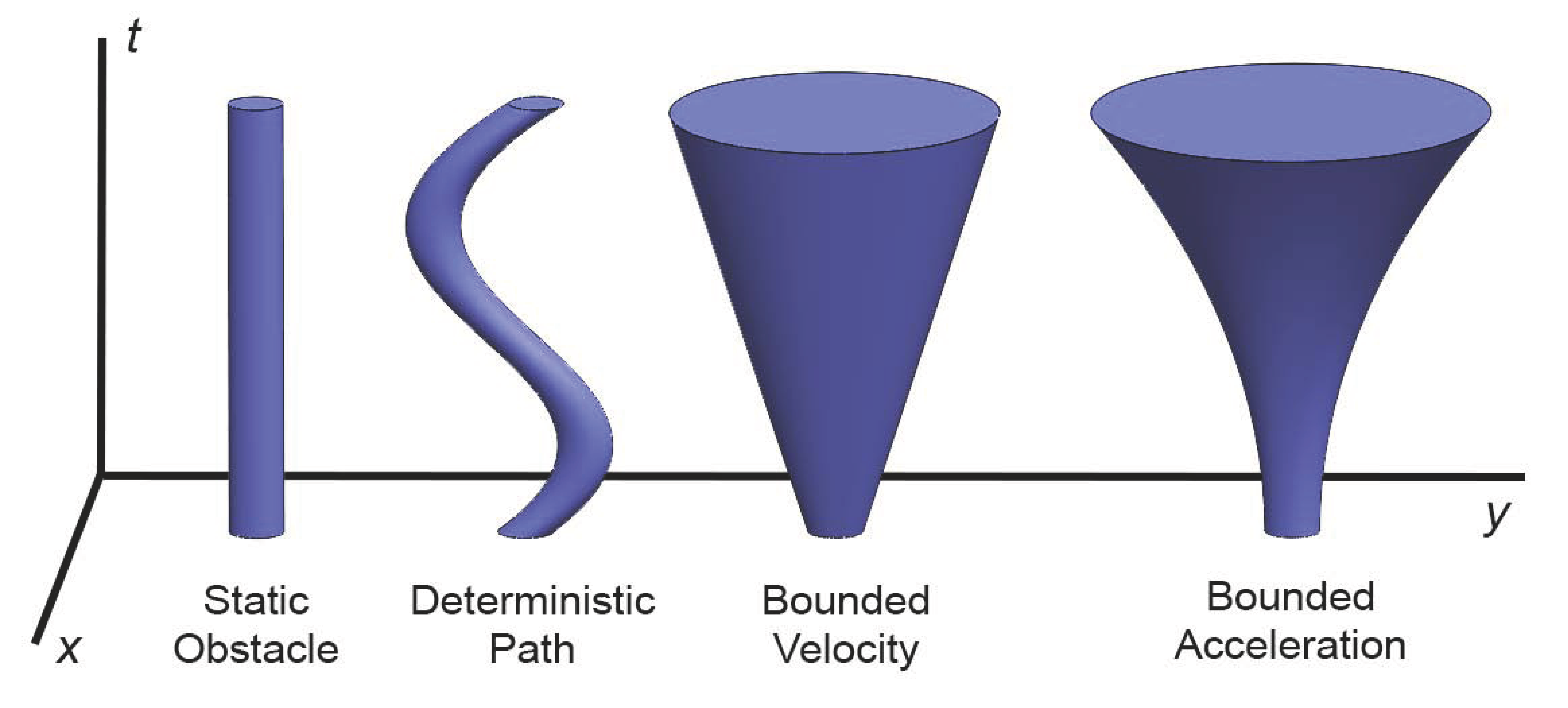
3.5.2. Planning in Space-Time

To better account for obstacle movement, it is necessary to include time as a dimension in the configuration space, which increases the problem complexity. Furthermore, while instantaneous position and velocity of obstacles may be perceived, it is yet difficult to ascertain future obstacle trajectories. Prior approaches have aimed to use simple assumptions, such as constant velocity trajectory, in predicting obstacle movement, with errors accounted for by rapid iterative re-planning. Other more conservative approaches have aimed to account for variations in obstacle trajectory by bounding larger obstacle-occupied sub-spaces within the configuration space, within which samples are rejected by the planner [234,235].

Given a situation in which the instantaneous position and velocity of obstacles can be observed, it logically follows that future obstacle trajectories can be predicted. The common assumption of deterministic constant velocity requires frequent verification or correction with each new observation. Another method is to assume a bounded velocity on obstacles and represent them as conical volumes in space-time, thus reducing the need for observation updating and re-planning [234]. Other assumptions can be applied to obstacles as well, such as static assumption, constant velocity assumption, bounded velocity, and bounded acceleration, each of which yields a bounded volume of a different shape in space-time [235]. A visualization of ${\mathsf{\Re }}^2$ configuration-space obstacle trajectory predictions over space-time is shown in Figure 4. A naive assumption would be to ignore the uncertainty in the prediction of an obstacle’s trajectory, in which case the obstacle bounded space does not grow over time (left two cases in Figure 4). A more conservative approach would be to assume a larger bounded area of possible obstacle occupancy, where the obstacle space bounds grow over time according to assumed limitations on the obstacle’s velocity and or acceleration (right two cases in Figure 4).

3.5.3. Control Space Obstacle Representations

Rather than check for collisions directly in the robot’s configuration space, another popular approach is to directly plan in the control space by prohibiting certain control actions which are predicted to lead to collision. For example, the velocity obstacles method assumes that obstacles will maintain their observed trajectories and forbids a robot from choosing relative velocities that would lead to collision with the obstacle’s current trajectory [236]. This was generally applied to circular, holonomic robots, but due to the ease of computation it has gained popularity in multi-robot planning, with proposed Reciprocal Velocity Obstacles [237]. Recent extensions to the velocity obstacles method have further incorporated acceleration constraints [238], and adjustments for nonholonomic robots [239].

3.6. Planning Subject to Differential Constraints

Motion planning is ultimately a high-level control problem. In practice, control limitations may be ignored to various degrees in the motion planner in the name of simplicity or reduction of computational burden, however poor accounting for constraints on the robot motion during the planning phase can lead to high control errors and result in trajectory inefficiencies and/or hazardous operations. Trajectories with longer path length which can be followed closely might have shorter execution times than shorter paths which are more difficult to follow in reality. Discrepancies between the planned trajectory and the executed trajectory present a danger since this lessens the validity of collision checking during the planning phase. Paths can be generated from directly sampling admissible controls [240], however these methods do not optimize paths through tree rewiring, and popular asymptotically optimal planners, such as RRT* [207] require sampling from the configuration space. Incorporating differential constraints into state-sampling planners is still a challenging matter, and requires a steering function to draw an optimal path between two given states which obeys control constraints (if such a path exists), as well as efficient querying methods to tell whether a sampled state is reachable from a potential parent state.

One of the most fundamental differential constraints in a system is the evolution of time, where time t must increase at a constant rate $\dot{t}=1$. Whether or not time is explicitly included as a state parameter, other state parameters will typically have differential constraints with respect to time, such as velocity and/or acceleration limits. Robot differential constraints are applied to generate velocity profiles, which may be solved for in a decoupled manner only over the chosen geometric path [241,242], or in a direct integrated manner simultaneously with geometric path solving over every connection in the tree as it is built [208,240,243,244,245]. Turning radius limitations are also common, where paths for car-like models are often solved through Dubins curves [246] or Reeds-Shepp curves [247], which are proven to have shortest distance given a minimum turning radius, though more sophisticated methods exist which also consider a weighted control effort heuristic [244]. Decoupled differential constraint handling can result in very inefficient trajectories or failure to find a trajectory due to the decoupling. Conversely, direct integrated differential constraint handling can overcome these shortcomings but is more computationally complex.

State sampling can be made more efficient by limiting the states that are sampled to only those from within a set of states known to be reachable from the initial condition given the robot’s kinodynamic constraints applied to an obstacle free environment. Likewise it is only beneficial to check for connectivity between neighboring states when they fall within each other’s reachable sets; checking any states that are nearby by Euclidean distance metric but not reachable within a short period of time given kinodynamic constraints is a waste of computational effort. Adding Reachability Guidance (RG) to state sampling and Nearest Neighbor (NN) searching can provide significant efficiency boosts to planning speed, especially for systems where motion is highly constrained or the motion checking cost is high, and the standard naive approaches of uniform sampling over a hyperrectangle and NN searching by Euclidean distance metric would otherwise result in slow planner performance.

Several recent works have presented analytical approaches to incorporate RG into motion planning. The asymptotic optimality of RRT* was shown to extend to a reachability guided variant where the reachable subspace was represented as a hyperrectangle derived from the linearized dynamics approximation of a system through the Ball Box Theorem presented in [243], where the “box” was an under-approximation of the true reachable subspace. A similar approach was taken in [245] to prove asymptotic optimality in differential constraint handling variants of PRM (Probabilistic RoadMaps) and FMT (Fast Marching Tree). Another asymptotically optimal sampling based algorithm to handle differential constraints, Goal-Rooted Feedback Motion Tree (GR-FMT) was presented in [248], limited in application to controllable linear systems with linear constraints. An analytical method for solving a two point boundary value problem subject to kinodynamic constraints was presented in [244], which could be used for finding optimal state-to-state connections and NN searching but was limited to systems with linear dynamics.

A machine learning approach was taken in [249] to query for whether a state was reachable from a given base state, though this method required applying a Support Vector Machine (SVM) classifier over a feature set of 36 features for the Dubins car model, where online solving for 36 features could be relatively computationally expensive.

The Reachability Guided RRT planner presented in [250] relied on construction of Voronoi diagrams to build approximations of reachable sets rooted from each graph node for sampling biasing, where Euclidean distance metric was still used for NN searching. This method may not easily be extended to higher dimensional spaces, as Voronoi diagrams are then no longer easily constructed.

There are also relatively few planning methods that have been demonstrated to be effective for solving over a configuration space with an appended time dimension. Early works explored control sampling approaches [240], and recent state sampling works have made model simplifications to handle the differential constraints in an online manner, such as keeping to a constant ego robot speed [251]. Others have performed planning by graph search over a discrete, time-bounded lattice structure built from motion primitives [252], or a grid cell decomposition of the state space [253], though these methods loose the benefits of sampling based approaches (which are less limited in resolution, and have potential for rewiring and optimization).

3.7. Incremental Planning and Replanning

Limited perception range and the dynamic nature of operating environments are common challenges for autonomous vehicle planning. The sensing range of the mobile robot is typically limited not only by sensor specifications, but also reduced by view obstruction in the presence of obstacles. It is often the case that the robot will not be able to perceive the entire route from a start location to goal location at any one specific instant of time. Thus the robot will need to generate incremental plans to follow trajectories which lead to forward progress towards the robot’s ultimate goal location. Furthermore, as the robot progressively executes its planned trajectory, other moving agents will have their own goals in mind and may move unexpectedly. Given a substantial environment change, robot trajectories that were believed to be safe at a prior time instance may not longer be safe at a subsequent time instance. Replanning is then necessary to adjust for dynamic changes to the environment.

Incremental planning requires a means of incrementally generating sub-goals, or otherwise choosing the best trajectory from amongst a set of possible trajectories based on some heuristics. A new plan must be generated at least as often as a new sub-goal is defined. In [242], a finite state machine generates new sub-goals for a sampling based replanner only when the robot was forced to come to a stop due to path blockage, where each subgoal was set at a predefined distance ahead along the predefined path. In [254], no sub-goals were defined, nor was there a predefined path to utilize, but rather the best choice trajectories were decided based on a combined weighted heuristic of trajectory execution time and distance to goal from the end trajectory state. Bouraine et al. [254] applied a constant rate replanning timer, where each current solution plan was executed concurrently while the subsequent plan was being generated, and each newly planned trajectory would be rooted from an anticipated committed pose given the previous committed solution trajectory. Note that in a Mobility-on-Demand (MoD) context, a mission planner should be able to provide a predefined path which leads from a starting point to an end destination based on a passenger service request, and the presence of a predefined path can help to overcome dangers of getting stuck due to local minima. Mobility-on-Demand (MoD) refers to vehicle sharing schemes whereby passenger services are provided to customers throughout a city with instant booking of vehicles available. A distributed MoD fleet is meant to provide responsive “first and last mile” transportation (short connections to rapid transit systems from unserviced areas), or other short distance trips, thereby reducing the need for private vehicle ownership by increasing public transportation accessibility.

Iteratively replanning to generate new solution trajectories presents a potential opportunity to carry over knowledge from previous planning iterations to subsequent planning iterations. While of course each new plan could start from scratch, better solutions may be found faster if prior planning information is well utilized. For example, sampling could be biased to sample near waypoints along the previously chosen solution path, as with Extended RRT (ERRT) [255]. Other works have suggested redoing collision-checks over the entire planning tree, as in Dynamic RRT (DRRT) [256], where the tree structure was utilized to trim child “branches” once a parent state was found to be no longer valid, and sampling is biased towards trimmed regions. Recently, a replanning variant of RRT* was presented, RRT${}^X$ [257], which trims the previous planning iteration’s planning tree in similar fashion to DRRT, but furthermore efficiently reconnects disconnected branches to other parts of the tree and maintains the rewiring principal of RRT* responsible for asymptotic optimality.

Safety mechanisms should also be carefully designed considering that each planning cycle requires a finite time for computation and the environment may change during that time (e.g., obstacles may change trajectories). Several works have prescribed passive safety mechanisms to reduce speed in response to obstacle presence, where passive safety refers to the ability to avoid collision while the robot is in motion (escaping from a hostile agent is a more advanced planning topic). In [258], spatial path planning was decoupled from velocity planning, and a “Dynamic Virtual Bumper” approach would prescribe reduced speed based on the proximity of the nearest obstacle as measured by a weighted longitudinal and lateral offset from the desired path. Moving obstacles were treated as enlarged static obstacles in [258], where the obstacles were assumed to occupy the area traced by their current constant velocity trajectory over a short time frame in addition to their current spatial location. While decoupled approaches are generally simpler to implement, they may give rise to inefficiencies, or even failure to find a solution when one exists by integrated planning problem formulation. Several other trajectory planning methods which consider spatial paths and velocity in an integrated manner were benchmarked for safety evaluation in [259], where Inevitable Collision State Avoidance (ICS-AVOID) [260], was deemed to outperform Non-Linear Velocity Obstacles (NLVO) [261] and Time-Varying Dynamic Window [262]. ICS-AVOID maintained a finite control set kernel to test over each trajectory’s end state to ensure that no executed trajectory would end in an ICS [260].

4. Control

The execution competency of an autonomous system, also often referred to as motion control, is the process of converting intentions into actions; its main purpose is to execute the planned intentions by providing necessary inputs to the hardware level that will generate the desired motions. Controllers map the interaction in the real world in terms of forces, and energy, while the cognitive navigation and planning algorithms in an autonomous system are usually concerned with the velocity and position of the vehicle with respect to its environment. Measurements inside the control system can be used to determine how well the system is behaving, and therefore the controller can react to reject disturbances and alter the dynamics of the system to the desired state. Models of the system can be used to describe the desired motion in greater detail, which is essential for satisfactory motion execution.

4.1. Classical Control

Feedback control is the most common controller structure found in many applications. Feedback control uses the measured system response and actively compensates for any deviations from the desired behavior. Feedback control can reduce the negative effects of parameter changes, modelling errors, as well as unwanted disturbances. Feedback control can also modify the transient behavior of a system, as well as the effects of measurement noise.

The most common form of classical feedback control is the Proportional-Integral-Derivative (PID) controller. The PID controller is the most widely used controller in the process control industry. The concept of PID control is relatively simple. It requires no system model, and the control law is based on the error signal as:

$$u\left(t\right)=k_d\dot{e}+k_{p}e+k_i\int e\left(t\right)dt$$

(2)

where e is the error signal, $k_p$, $k_i$ ,and $k_d$ are the proportional, integral, and derivative gains of the controller, respectively.

However, the use of only feedback terms in a controller may suffer from several limitations. The first significant limitation of a feedback only controller is that it has delayed response to errors, as it only responds to errors as they occur. Purely feedback controllers also suffer from the problem of coupled response, as the response to disturbances, modelling error, and measurement noise are all computed by the same mechanism. It is more logical then to manipulate the response to a reference independently from the response to errors.

Another degree of freedom can be added to the controller by including a feedforward term to the controller, where this controller architecture is shown in Figure 5. The addition of a feedforward term in the controller can help to overcome the limitations of feedback control. The feedforward term is added to the control signal without considering any measurement of the controlled system. However, the feedforward term may involve the measurement of disturbances, etc. Designing a feedforward control requires a more complete understanding of the physical system, and therefore, oftentimes, a model reference is used for the feedforward controller. The method of combining a feedforward and a feedback term in the controller is also known as two degree of freedom controller.

Table 1. Feedforward vs Feedback Control.

	Feedback	Feedforward
Removes Unpredictable Errors and Disturbances	(+) yes	(−) no
Removes Predictable Errors and Disturbances	(−) no	(+) yes
Removes Errors and Disturbances Before They Happen	(−) no	(+) yes
Requires Model of a System	(+) no	(−) yes
Affects Stability of the System	(−) yes	(+) no

summarizes the roles of feedforward and feedback control [143].

State space control, often referred to as modern control, is a technique that tries to control the entire vector of the system as a unit by examining the states of the system. The field of state space control is a very large field and there is still much active ongoing research in this area. A linear state space model can be written as:

$$\dot{x\left(t\right)}=A\left(t\right)x\left(t\right)+B\left(t\right)u\left(t\right)y\left(t\right)=C\left(t\right)x\left(t\right)+D\left(t\right)u\left(t\right)$$

(3)

where $x\left(t\right)$ is the system state vector, $u\left(t\right)$ is the control input vector, and $y\left(t\right)$ is the output of the system.

The observations in an autonomous system are mostly nonlinear, and therefore a linear model of the nonlinear system may have to be produced by first linearizing the state space equation of the system.

$$\dot{x\left(t\right)}=f(x\left(t\right),u\left(t\right))y\left(t\right)=h(x\left(t\right),u\left(t\right))$$

(4)

The two degree of freedom controller can also be applied to nonlinear systems. Feedforward is used to generate a reference trajectory, while the feedback is used to compensate for disturbances and errors.

The nonlinear system can be linearized about a reference trajectory $x_r\left(t\right)$ to produce linearized error dynamics.

$$\delta \dot{x\left(t\right)}=A\left(t\right)\delta x\left(t\right)+B\left(t\right)\delta u\left(t\right)\delta y\left(t\right)=C\left(t\right)\delta x\left(t\right)+D\left(t\right)\delta u\left(t\right)$$

(5)

where $A,B,C,$ and D are the appropriate Jacobians. If there exists a trajectory generation process that can be designed to produce a reference input $u_r\left(t\right)$, such that $u_r\left(t\right)$ generates a feasible trajectory which satisfies the nonlinear system dynamics of the system, state space controllers can be configured to perform feedback compensation for the linearized error dynamics.

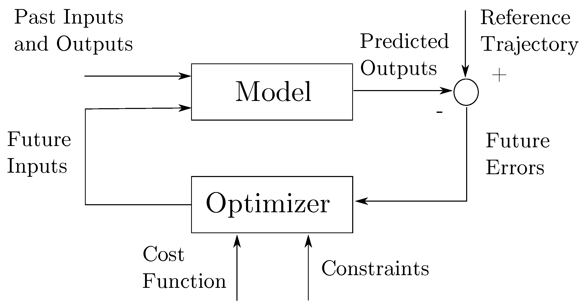
4.2. Model Predictive Control

Autonomous systems need motion models for planning and prediction purposes. Models can also be used in control execution. A control approach which uses system modelling to optimize over a forward time horizon is commonly referred to in the literature as Model Predictive Control (MPC). The basic structure of MPC is shown in Figure 6. Model predictive control has been developed to integrate the performance of optimal control and the robustness of robust control. Typically the prediction is performed for a short time horizon called the prediction horizon, where the goal of the model predictive controller is to compute the optimal solution over this prediction horizon. The model, and thus the controller can be changed online to adapt to different conditions.

Model predictive control has seen tremendous success in the industrial process control applications, due mainly to its simple concept and its ability to handle complicated process models with input constraints and nonlinearities [263].

Model predictive control has several other attractive features, such as the simplicity of designing a multi variable feedback controller. It also allows for easy specification of system inputs, states, and outputs that must be enforced by the controller. MPC furthermore permits specification of an objective function to optimize the control effort. MPC can also address time delay, rejecting measured and unmeasured disturbances and taking advantage of previously stored information of expected future information. This feature can be very useful for repeated tasks, such as following a fixed path. MPC embodies both optimization and feedback adjustment, thus mimicking natural processes.

Model predictive control has also been widely adapted to automotive applications [264]. The operations of the overall vehicle system must be optimal throughout the operating range in order to increase the fuel economy, emission, and safety performance. However, applying a model predictive controller in an automotive system meets different challenges than those faced in the process control industry. In the process control industry, the sampling time is relatively longer, and the computing resources available are ample. The sampling period for processes in an automobile is a few milliseconds, and the amount of computing resources available is limited due to space constraints. Advances in processor speed and memory, as well as development of new algorithms is therefore important in pushing the adoption of MPC into greater prevalence in the automotive industry.

MPC has already been applied in several automotive control applications, including traction control [265], braking and steering [266,267], lane keeping [268] etc. Model predictive techniques have also been applied to the trajectory tracking problem in various works [269,270,271,272,273,274,275].

The general model predictive control problem is formulated as

$$\begin{array}{cccc}\hfill & \underset{U\left(t\right)}{\mathrm{minimize}}\hfill & & F\left(x\left(N\right|t)\right)+\sum _{k=0}^{N-1}L(x\left(k\right|t),y\left(k\right|t),u\left(k\right|t))\hfill \end{array}$$

(6)

$$\begin{array}{cccc}& \mathrm{subject}\mathrm{to}\hfill & & x(k+1|t)=f(x\left(k\right|t),u(k\left|t\right))\hfill \end{array}$$

(7)

$$\begin{array}{cccc}& & & y\left(k\right|t)=h(x\left(k\right|t),u(k\left|t\right))\hfill \end{array}$$

(8)

$$\begin{array}{ccccc}& & & x_{min}\le x\left(k\right|t)\le x_{max},\hfill & \hfill k=1,\cdots ,N_c\end{array}$$

(9)

$$\begin{array}{ccccc}& & & y_{min}\le y\left(k\right|t)\le y_{max},\hfill & \hfill k=1,\cdots ,N_c\end{array}$$

(10)

$$\begin{array}{ccccc}& & & u_{min}\le u\left(k\right|t)\le u_{max},\hfill & \hfill k=1,\cdots ,N_{cu}\end{array}$$

(11)

$$\begin{array}{cccc}& & & x\left(0\right|t)=x(t)\hfill \end{array}$$

(12)

$$\begin{array}{ccccc}& & & u\left(k\right|t)=\kappa (x\left(k\right|t\left)\right)\hfill & \hfill k=N_u,\cdots ,N-1\end{array}$$

(13)

where t is the discrete time index. The notation for a vector $v\left(h\right|t)$ denotes the value for v predicted at h time steps as referenced from time t, based on information up to t. Equations (7) and (8) are the discrete time model of the system dynamics with sampling period $T_s$ where $x\in {\mathsf{\Re }}^n$ is the system’s state, $u\in {\mathsf{\Re }}^m$ is the control input, and $y\in {\mathsf{\Re }}^p$ is the system output. The optimizer is the control input sequence $U\left(t\right)=\left(u\right(0\left|t\right),\cdots ,u(N-1|t\left)\right)$, where N is the prediction horizon. Similar to the optimal control formulation, the cost function represents the performance objective that consists of the stage cost L and the terminal cost F. The constraints on the states and outputs are enforced along the horizons $N_c$ and $N_{cu}$, respectively. The control horizon $N_u$ is given as the number of optimized steps before the terminal control law is applied.

At any control cycle t, the model predictive control strategy for the general problem operates as follows: system outputs are measured and the state $x\left(t\right)$ is estimated. This state estimation is acquired to initialize Equation (6) and impose the limit in Equation (12). Once the MPC optimization problem is solved and the optimal input sequence $U^{*}\left(t\right)$ is obtained, the first element of the optimal input sequence is then applied to the system $u\left(t\right)=u^{*}\left(0\right|t)$. At the following cycle, the process is repeated using the newly acquired state estimate, thus applying the feedback.

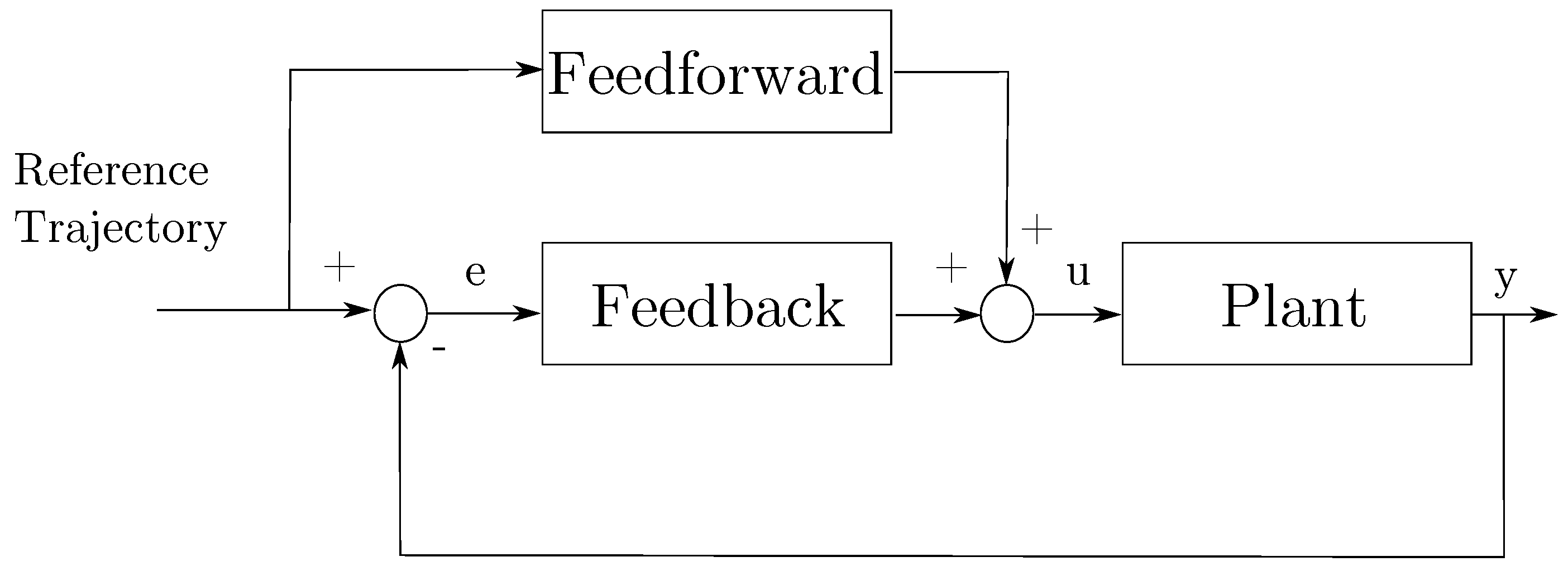
4.3. Trajectory Generation and Tracking

There are two general approaches to trajectory generation with known path information. The first approach uses the optimization method to both generate a trajectory and track it simultaneously, while another approach is to decouple trajectory generation and tracking.

4.3.1. Combined Trajectory Generation and Tracking

The combined approach integrates both the generation and execution/tracking tasks into one optimization problem. This approach is often applied for optimal time application such as in [276]. Running the optimization problem in real time is a challenge due to limited processing power, and it may not be advantageous for planning in a complex environment.

4.3.2. Separate Trajectory Generation and Tracking

Trajectory Generation

The problem of trajectory generation is to find an entire control input $u\left(t\right)$, which corresponds to some desired state trajectory $x\left(t\right)$.

The trajectory generation problem can be posed as a two point boundary value problem. The boundary conditions are typically the constraints that include a starting state $x\left(t_0\right)=x_0$ and the final goal state $x\left(t_f\right)=x_f$, with the system dynamics $\dot{x}=f(x,u)$ as an added constraint. A trajectory is defined as infeasible if there is no control input $u\left(t\right)$ for a given state trajectory $x\left(t\right)$ which satisfies the boundary conditions.

A trajectory is a representation of a motion confined to some time interval. This could be a specification of the state vector over an interval $\left\{x\left(t\right)|(t_0,t<t_f)\right\}$, or a specification of the input over an interval $\left\{u\left(t\right)|(t_0,t<t_f)\right\}$.

The problem of trajectory generation for an autonomous vehicle can be solved with multiple techniques. However, the literature for trajectory generation can generally be classified into two approaches: (i) sensor based and (ii) dynamics based. The first approach is more oriented towards the field of robotics. Robotics researchers have been tackling the problem of trajectory generation for decades, where it has been applied in both industrial robots and autonomous mobile robots. The sensor based approach generally concentrates on integrating the perception of the environment, without taking much of the vehicle dynamics into account.

Another approach to trajectory generation for an autonomous vehicle is based more on vehicle dynamics. Various optimization methods for finding an optimal trajectory have been proposed in the literature, such as the application of genetic algorithms, and gradient descent method. A deep understanding in vehicle dynamics and control can push the limits of the autonomous vehicle, as demonstrated in [277]. Research in trajectory generation and tracking is also pursued for application in semi-autonomous vehicles, for more advanced driver’s assistance systems, such as advanced collision avoidance with stability control [278,279,280].

A good balance between the sensor based trajectory planning and the vehicle dynamics control methods should be considered to fully realize the goal of autonomous vehicle control systems: to ensure that the vehicle can track the desired trajectory well, and operate safely, comfortably, and efficiently for all potential operating complexities and velocities.

Trajectory Tracking

In this section, an overview of the available path and trajectory tracking methods will be discussed. We consider a path to be a geometric representation of a plan to move from a start pose to a goal pose, whereas a trajectory additionally includes the velocity information of the motion. Various methods have been presented in the literature. Two of the most popular types are (i) geometric methods; and (ii) model based methods [281]. Controllers derived from model based path tracking methods use a kinematic and/or dynamic model of the vehicle. Kinematic model based controllers perform well at low speed applications, but the error increases as the vehicle speed and curvature rate of the path increases. On the other hand, the dynamic model based controllers tend to perform well for higher speed driving applications such as autonomous highway driving, but also tend to cut corners as the vehicle rapidly accelerates and decelerates and pursues paths with large curvature. Model based methods require the path to be continuous, and are not robust to disturbances and large lateral offsets.

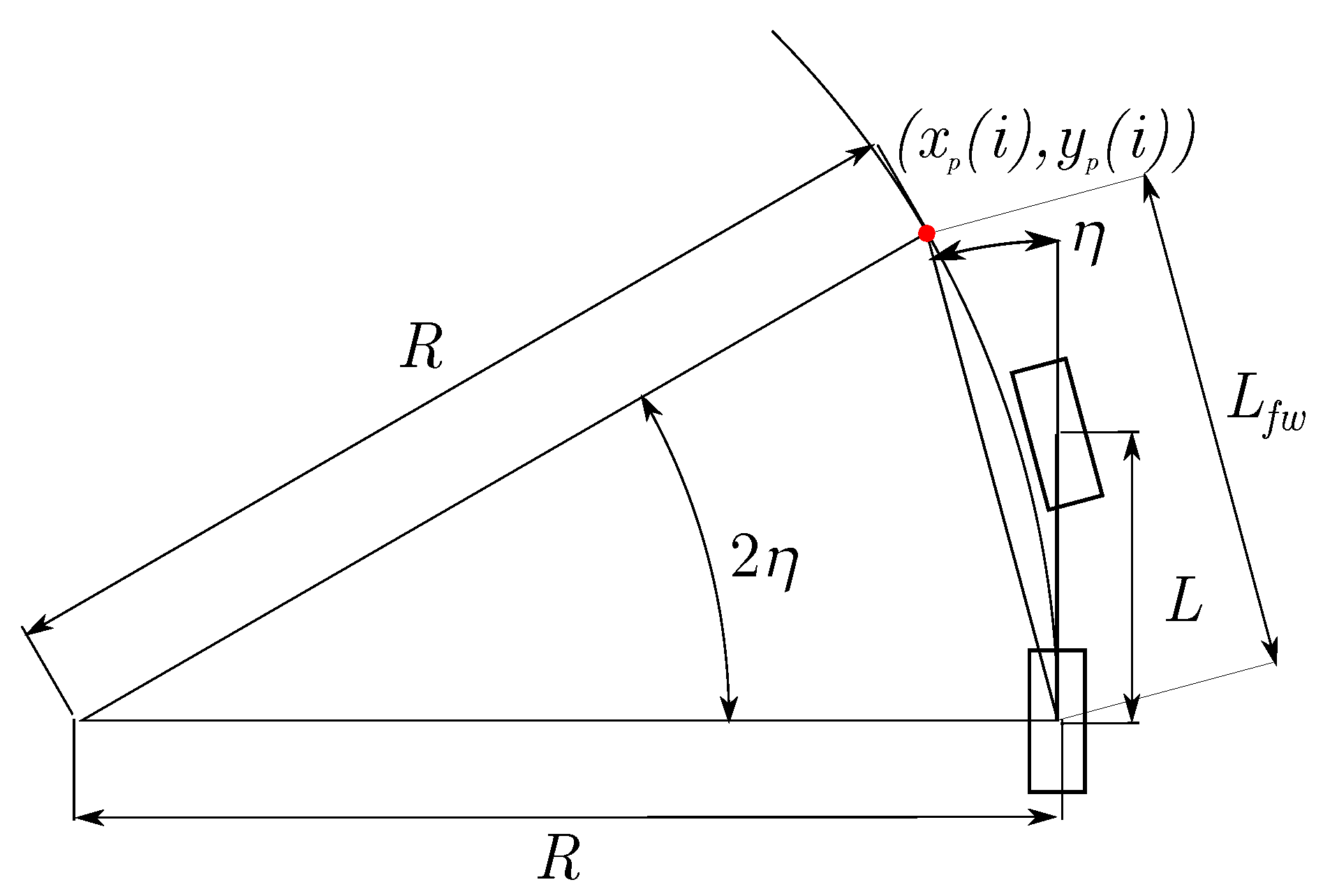
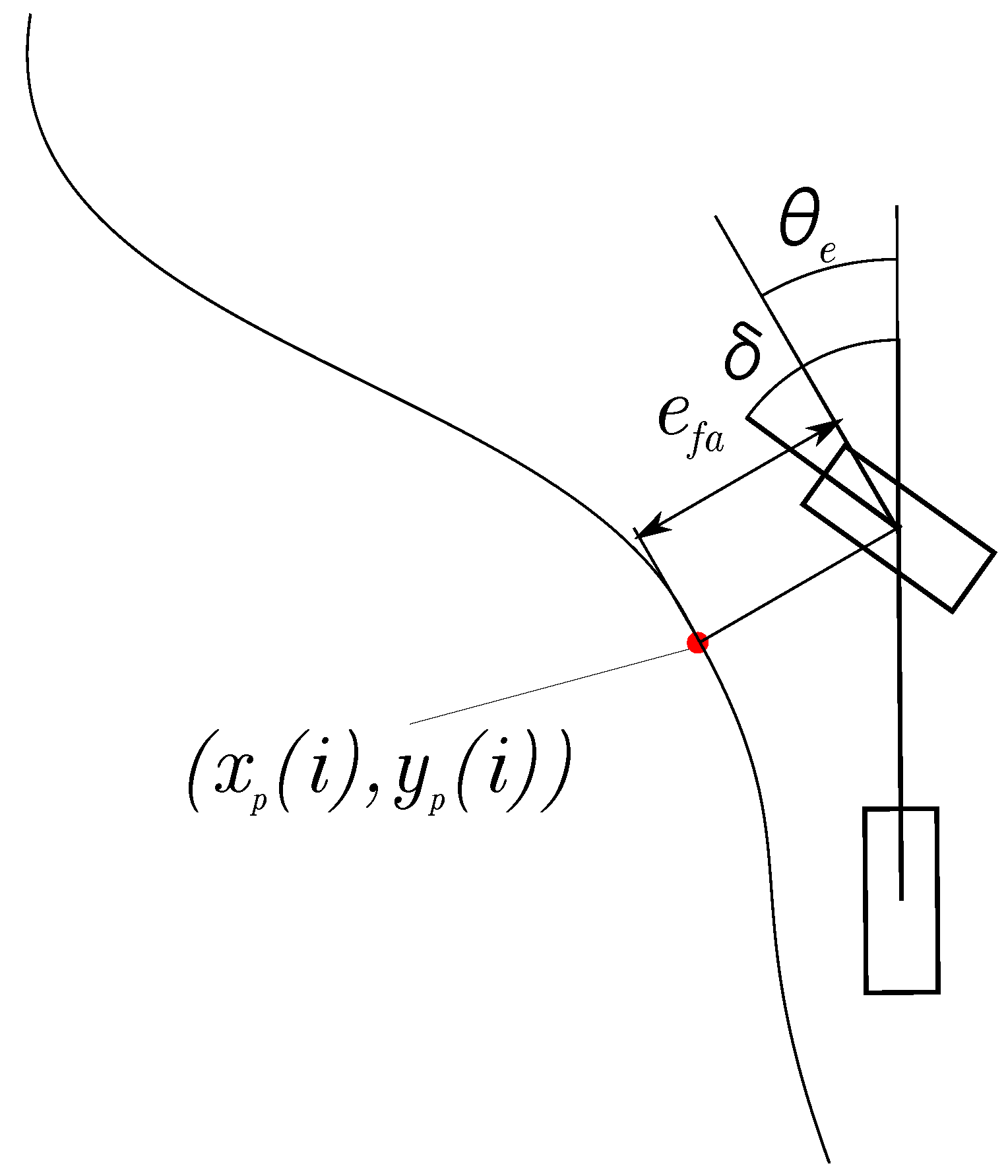
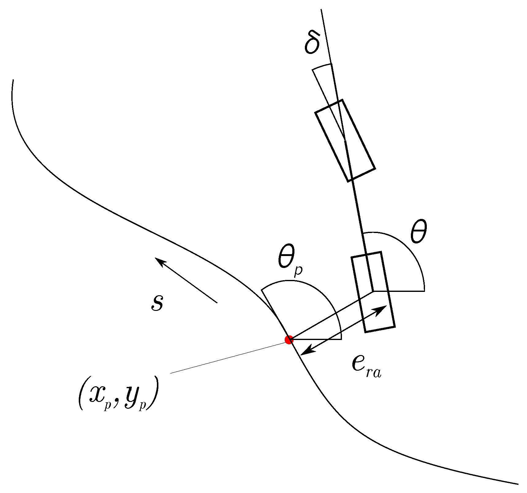
Geometric Path Tracking

Geometric path tracking algorithms use simple geometric relations to derive steering control laws. These techniques utilize look ahead distance to measure error ahead of the vehicle and their complexity range from simple circular arc calculations to much more sophisticated geometric theorems, such as the vector pursuit method [282].

One of the most popular geometric path tracking algorithms is the pure pursuit path tracking algorithm. The pure pursuit algorithm pursues a point along the path that is located at a certain lookahead distance away from the vehicle’s current position. The algorithm is relatively simple and easy to implement, and is robust to disturbances and large lateral error. The input to the algorithm is also waypoints, rather than smooth curves, and is therefore less susceptible to discretization related issues. This algorithm still suffers from corner cutting and steady state error problems if the lookahead distance selected is not appropriate, especially at higher speed, when the lookahead distance increases (lookahead distance is generally set as an increasing function with respect to speed).

In order to avoid constricting the way that the paths are generated, the paths shall be represented in a piece wise linear way [283]. By this principle, a smooth trajectory having continuous first and second order derivatives, e.g., a Bezier curve should be represented as a sequence of dense points, enabling a wider range of potential tracking algorithms to be applied. A point is joined to the following point in the path by linear path segments. In order to closely approximate the continuous path, a denser discretization of the path has to be implemented. The discrete nodes are contained in an ordered list, and the waypoints are tracked sequentially (waypoint i is tracked before waypoint $i+1$).

The pure pursuit algorithm has a single tunable parameter, the lookahead distance $L_{fw}$. Using Ackermann steering geometry, the algorithm defines a virtual circular arc that connects the anchor point (the rear axle) to the tracked point found along the path that is located $L_{fw}$ away from the anchor point. A variation of this algorithm has been introduced by [284], where the anchor point is not necessarily selected as the rear axle, but can be located at a distance ϵ away from the rear axle along $x_b$. However, hereafter, the anchor point will be assumed to be the rear axle. The stability limits of the algorithm has also been studied in [285], and it has been shown that the pure pursuit algorithm is stable for a correct combination of minimum lookahead distance and process delay involved in the system.

The virtual arc is constrained to be tangential to the velocity vector at the origin of the body fixed frame and to pass through the tracked point found along the path. Referring to Figure 7 and using the law of sines, the arc’s radius of curvature R can be geometrically computed as:

$$\begin{array}{c}\frac{L_{fw}}{sin\left(2\eta \right)}=\frac{R}{sin(\frac{\pi }{2}-\eta )}\\ \frac{L_{fw}}{2sin\left(\eta \right)cos\left(\eta \right)}=\frac{R}{cos\left(\eta \right)}\\ \frac{L_{fw}}{sin\left(\eta \right)}=2R\end{array}$$

where R is the turning radius, and η is the lookahead heading. The curvature κ of the arc is defined as:

$$\kappa =\frac{2sin\left(\eta \right)}{L_{fw}}$$

(14)

Therefore, the vehicle’s steering angle δ can be computed by applying the kinematic bicycle model:

$$\delta =ta{n}^{-1}\left(\kappa L\right)$$

$$\delta \left(t\right)=ta{n}^{-1}\left(\frac{2Lsin\left(\eta \right(t\left)\right)}{L_{fw}}\right)$$

(15)

The lookahead distance is commonly formulated as a function of longitudinal velocity, and saturated at a certain maximum and minimum value, and thus Equation (15) can be rewritten as

$$\delta \left(t\right)=ta{n}^{-1}\left(\frac{2Lsin\left(\eta \right(t\left)\right)}{kv\left(t\right)}\right)$$

(16)

At lower speed, when the lookahead distance is smaller, the vehicle is expected to track the path closely, and oscillatory behavior is also expected; meanwhile at higher velocity, when the lookahead distance is larger, the vehicle is expected to track the path smoothly, however this will result in the cutting corner problem.

Since the lookahead distance is a function of the gain k, selecting the appropriate value for the gain will result in significant trade-offs in the tracking performance. On one hand, if the gain k is set to be too low, the algorithm will track a point that is very close to the vehicle’s current pose. As the vehicle’s control may not be perfect, a vehicle tracking a constant curvature path may oscillate between being inside and outside of the curve; this can result in steering control towards the opposite direction, and therefore instability may occur. On the other hand, if the gain k is set to be too large, the opposite effect is expected. The autonomous vehicle is expected to stay inside/outside of the curve for a very long time rather than moving closer and closer to the curvature, and therefore poor tracking performance is expected.

Tuning the pure pursuit controller to achieve a good path tracking result which minimizes the corner cutting and overshoot problems can be a tedious and course dependent challenge. One of the main reasons is that the pure pursuit path tracking algorithm does not consider the target path curvature, and the heading of the tracked point along the path. The pure pursuit algorithm simply calculates a circular arc based on the geometry of the vehicle model. Ignoring the vehicle’s lateral dynamics that are more and more influential as the speed increases, which results in discrepancies between the predicted circular arc and the actual travelled circular arc. This dynamic effect can be compensated by increasing the gain k until the circular arc that is computed is of smaller radius than the circular arc of the path at a proportion that would cancel out the dynamic side slip of the vehicle.

The Stanley method is another popular geometric steering controller that was first introduced with Stanford University’s entry in the DARPA Urban Challenge [286].

Referring to Figure 8, the Stanley method computes the steering command based on a nonlinear control law which considers the cross track error $e_{fa}$ measured from the center of the front axle of the vehicle to the path at $(x_p,y_p)$, as measured from the front axle of the vehicle, as well as the heading error ${\theta }_e$ of the vehicle with respect to the path:

$${\theta }_e=\theta -{\theta }_p$$

(17)

where θ is the heading of the vehicle, and ${\theta }_p$ is the heading of the path. The resulting control law for the steering angle δ can be written as:

$$\delta \left(t\right)={\theta }_e\left(t\right)+ta{n}^{-1}\left({\displaystyle \frac{k{e}_{fa}\left(t\right)}{v_x\left(t\right)}}\right)$$

(18)

The second term in Equation (18) adjusts the steering angle such that the intended trajectory intersects the path at ${\displaystyle \frac{v_x\left(t\right)}{k}}$ distance away from the path tangent to $(x_p,y_p)$, where k is the gain parameter and $v_x\left(t\right)$ is the instantaneous longitudinal velocity of the vehicle.

The algorithm has been proven to exponentially converge to zero cross track error. Compared to the pure pursuit method, the Stanley method, has better tracking results and does not cut corners as it uses cross track error and yaw heading error information of the vehicle with respect to the path as measured from the front axle rather than pursuing a point that is located at a certain distance ahead of the vehicle. It also performs better at high speed driving as compared against the pure pursuit method.

However, the Stanley method is not as robust to disturbances, and has higher tendency for oscillation as compared to the pure pursuit method, as it only considers the current cross track error rather than considering the path ahead. In instances where the controller is not ideal, tracking a constant curvature path with the Stanley method may result in similar symptoms as tracking the path with a pure pursuit controller with small lookahead distance. The vehicle’s position may oscillate between the inside and the outside of the curvature, and the computed steering angle may oscillate between positive and negative values (left or right). The Stanley method also requires continuous curvature path rather than discrete waypoints, as it considers the cross track error in a continuous manner, which makes it susceptible to discretization related problems [287].

Trajectory Tracking with a Model

For a given path/trajectory there are several model based tracking methods to choose from. At slower speeds, vehicle kinematics models or linearized dynamics are often used. When attempting stability in control at higher velocity, a more complex model is usually required.

De Luca, Oriolo, and Samson [288] have proposed a kinematic car controller based on the kinematic bicycle model. This method can apply not only to car like robots, but also to many other kinematic models for various mobile robots.

Referring to Figure 9, De Luca et al. defined the path according to a function of its length s. Let ${\theta }_p\left(s\right)$ represent the angle between the path tangent at $(x_p,y_p)$ and the global x axis. Orientation error ${\theta }_e$ of the vehicle with respect to the path is then defined as

$${\theta }_e=\theta -{\theta }_p\left(s\right)$$

and the curvature along the path is defined as:

$$\kappa \left(s\right)={\displaystyle \frac{e_{ra}{\theta }_p\left(s\right)}{ds}}$$

multiplying both sides by $\dot{s}$

$${\dot{\theta }}_p\left(s\right)=\kappa \left(s\right)\dot{s}$$

Given that cross track error $e_{ra}$ is the orthogonal distance from the anchor point (midpoint of the rear axle) to the path, the quantities $\dot{s}$ and ${\dot{e}}_{ra}$ can be expressed as

$$\begin{array}{cc}\hfill \dot{s}& =vcos\left({\theta }_e\right)+{\dot{\theta }}_p{e}_{ra}\hfill \\ \hfill \dot{e_{ra}}& =vsin\left({\theta }_e\right)\hfill \end{array}$$

The kinematic model in path coordinates can now be written as

$$\left[\begin{array}{c}\dot{s}\\ {\dot{e}}_{ra}\\ {\dot{\theta }}_e\\ \dot{\delta }\end{array}\right]=\left[\begin{array}{c}\frac{cos\left({\theta }_e\right)}{1-{\dot{e}}_{ra}\kappa \left(s\right)}\\ sin\left({\theta }_e\right)\\ \left(\frac{tan\delta }{L}\right)-\frac{\kappa \left(s\right)cos\left({\theta }_e\right)}{1-{\dot{e}}_{ra}\kappa \left(s\right)}\\ 0\end{array}\right]v\left[\begin{array}{c}0\\ 0\\ 0\\ 1\end{array}\right]\dot{\delta }$$

(19)

Canonical forms for kinematic models of nonholonomic systems are commonly used in controller design. One particular canonical structure that is used in deriving the controller is the chained form, intended for general two input systems such as the driftless kinematic car model. The chained form can be written as:

$$\begin{array}{cc}\hfill {\dot{x}}_1& =u_1\hfill \end{array}$$

(20)

$$\begin{array}{cc}\hfill {\dot{x}}_2& =u_2\hfill \end{array}$$

(21)

$$\begin{array}{cc}\hfill {\dot{x}}_3& =x_2{u}_1\hfill \end{array}$$

(22)

$$\begin{array}{c}\hfill ⋮\end{array}$$

(23)

$$\begin{array}{cc}\hfill {\dot{x}}_n& =x_{n-1}{u}_1\hfill \end{array}$$

(24)

where x represents state variable, and u represents input to the system. The problem can be further simplified as a single input system by assigning the first control input $u_1$ to be a function of time. Murray in [289] has proposed a way of converting the kinematic car model into the chained form, by a change of coordinates $x=\varphi \left(q\right)$ and invertible transformation $v=\beta \left(q\right)u$. The kinematic car model can then be put into chained form by using the following coordinate change:

$$\begin{array}{cc}\hfill x_1& =s\hfill \\ \hfill x_2& ={\kappa }^{\prime }\left(s\right)e_{ra}tan\left({\theta }_e\right)-\kappa \left(s\right)(1-e_{ra}\kappa \left(s\right)){\displaystyle \frac{1+si{n}^2\left({\theta }_e\right)}{co{s}^2\left({\theta }_e\right)}}+{\displaystyle \frac{(1-e_{ra}\kappa \left(s\right))tan\left(\delta \right)}{Lco{s}^3\left({\theta }_e\right)}}\hfill \\ \hfill x_3& =(1-e_{ra}\kappa \left(s\right))tan\left({\theta }_e\right)\hfill \\ \hfill x_4& =e_{ra}\hfill \end{array}$$

and the input transformation

$$\begin{array}{cc}\hfill v& ={\displaystyle \frac{1-e_{ra}\kappa \left(s\right)}{cos\left({\theta }_e\right)}}{u}_1\hfill \\ \hfill \dot{\delta }& ={\alpha }_2(u_2-{\alpha }_1{u}_1)\hfill \end{array}$$

where ${\alpha }_1$ and ${\alpha }_2$ are defined as

$$\begin{array}{cc}\hfill {\alpha }_1& ={\displaystyle \frac{\partial x_2}{\partial s}}+{\displaystyle \frac{\partial x_2}{\partial e_{ra}}}(1-e_{ra}\kappa \left(s\right))tan\left({\theta }_e\right)+{\displaystyle \frac{\partial x_2}{\partial {\theta }_e}}\left({\displaystyle \frac{tan\left(\delta \right)(1-e_{ra}\kappa \left(s\right))}{Lcos\left({\theta }_e\right)}}-\kappa \left(s\right)\right)\hfill \\ \hfill {\alpha }_2& ={\displaystyle \frac{Lco{s}^3\left({\theta }_e\right)co{s}^2\left(\delta \right)}{{(1-e_{ra}\kappa \left(s\right))}^2}}\hfill \end{array}$$

De Luca et al then proposed the following smooth feedback stabilization method. Their method takes advantage of the internal structure of the chained form and breaks the design solution into two phases. The first phase assumes that one control input is given, while the additional control input is used to stabilize the remaining sub-vector of the system state. The second phase consists of specifying the first control input to guarantee convergence and stability.

The variables of the chained form are reordered for simplicity as

$$\chi =({\chi }_1,{\chi }_2,{\chi }_3,{\chi }_4)=(x_1,x_2,x_3,x_4)$$

so the the chained form system can be written as

$$\begin{array}{cc}\hfill {\dot{\chi }}_1& =u_1\hfill \end{array}$$

(25)

$$\begin{array}{cc}\hfill {\dot{\chi }}_2& ={\chi }_3{u}_1\hfill \end{array}$$

(26)

$$\begin{array}{cc}\hfill {\dot{\chi }}_3& ={\chi }_4{u}_1\hfill \end{array}$$

(27)

$$\begin{array}{cc}\hfill {\dot{\chi }}_4& =u_2\hfill \end{array}$$

(28)

The ordering of $x_2$ and $x_4$ is made such that the position of the rear axle is $({\chi }_1,{\chi }_2)$. Let $\chi =({\chi }_1,{\chi }_2)$, where ${\chi }_2=({\chi }_2,{\chi }_3,{\chi }_4)$, and the goal is to stabilize ${\chi }_2$ to zero. ${\chi }_1$ represents the arc length s along the path, while ${\chi }_2$ represents the cross track error $e_{ra}$, and ${\chi }_3,{\chi }_4$ are related to the steering angle and orientation error of the tracked path respectively.

If $u_1$ is assigned as a function of time, the chained system can be written as

$$\begin{array}{c}\hfill {\dot{\tilde{\chi }}}_2=0\\ \hfill \dot{{\chi }_2}=\left[\begin{array}{ccc}0& u_1\left(t\right)& 0\\ 0& 0& u_1\left(t\right)\\ 0& 0& 0\end{array}\right]{\chi }_2+\left[\begin{array}{c}0\\ 0\\ 1\end{array}\right]u_2\end{array}$$

with

$${\tilde{\chi }}_1={\chi }_1-{\int }_0^t{u}_1\left(t\right)dt$$

When $u_1$ is assigned a priori, ${\tilde{\chi }}_1$ is not controllable. However, the structure of the differential equation for ${\chi }_2$ is similar to the controllable canonical form that is widely studied in state space control. The system also becomes time invariant as $u_1$ is set at a constant non-zero value. If $u_1$ is a piecewise continuous, bounded, and strictly positive/negative function, then ${\chi }_2$ is controllable. Under this assumption

$${\displaystyle \frac{d}{dt}}{x}_1={\displaystyle \frac{d}{d{\chi }_1}}\dot{{\chi }_1}={\displaystyle \frac{d}{d{\chi }_1}}{u}_1$$

$$sign\left(u_1\right){\displaystyle \frac{d}{d{\chi }_1}}\dot{{\chi }_1}={\displaystyle \frac{1}{|u_1|}}.{\displaystyle \frac{d}{dt}}$$

and thus the state space equation can be rewritten as

$$\begin{array}{cc}\hfill {\chi }_2^{\left[1\right]}& =sign\left(u_1\right){\chi }_3\hfill \end{array}$$

(29)

$$\begin{array}{cc}\hfill {\chi }_3^{\left[1\right]}& =sign\left(u_1\right){\chi }_4\hfill \end{array}$$

(30)

$$\begin{array}{cc}\hfill {\chi }_4^{\left[1\right]}& =sign\left(u_1\right)u_2^{\prime }\hfill \end{array}$$

(31)

By applying the definition

$$\begin{array}{cc}\hfill {\chi }_i^{\left[j\right]}& =sign\left(u_1\right){\displaystyle \frac{d^j{\chi }_i}{d{\chi }_1^j}}\hfill \\ \hfill u_2^{\prime }& ={\displaystyle \frac{u_2}{u_1}}\hfill \end{array}$$

the system has an equivalent input-output representation of

$$\begin{array}{cc}\hfill {\chi }_2^{\left[n-1\right]}& =sign{\left(u_1\right)}^{n-1}{u}_2^{\prime }\hfill \end{array}$$

and the system is controllable, admitting an exponentially stable linear feedback in the form of

$$\begin{array}{c}\hfill u_2^{\prime }\left({\chi }_2\right)=-sign{\left(u_1\right)}^{n-1}\sum _{i=1}^{n-1}{k}_i{\chi }_2^{\left[i-1\right]}\end{array}$$

where the gain $k_1>0$ for stability, and the time varying control

$$\begin{array}{c}\hfill u_2({\chi }_2,t)=u_1\left(t\right)u_2^{\prime }\left({\chi }_2\right)\end{array}$$

is globally asymptotically stable at the origin ${\chi }_2=0$.

The goal of the path tracking problem is to bring ${\chi }_2,{\chi }_3,and{\chi }_4$ down to zero, the solution to the path tracking problem for an Ackermann steered vehicle for any piecewise continuous, bounded and strictly positive/negative $u_1$ can be written as:

$$\begin{array}{c}\hfill u_2^{\prime }({\chi }_2,{\chi }_3,{\chi }_4)=-sign\left(u_1\right)\left[k_1{\chi }_2+k_{2}sign\left(u_1\right){\chi }_3+k_3{\chi }_4\right]\end{array}$$

and the final path tracking feedback control law can be obtained as

$$\begin{array}{c}\hfill u_2({\chi }_2,{\chi }_3,{\chi }_4,t)=-k_1|u_1\left(t\right)|{\chi }_2-k_2{u}_1\left(t\right){\chi }_3-k_3\left|u_1\left(t\right)\right|{\chi }_4\end{array}$$

Model predictive techniques have also been applied to trajectory tracking problem. The main challenge with model predictive approaches in trajectory tracking and control is that the nonlinear optimization problem has to be solved several times per second. With recent advances in available computational power, solving nonlinear optimization in real time is now feasible. A few variations of the MPC problem for trajectory tracking that can be found in the literature are as follows:

• Path Tracking Model Predictive Controller : with a center of mass based linear model, Kim et al. [290] formulated an MPC problem for a path tracking and steering controller. The resulting integrated model is simulated with a detailed automatic steering model and a vehicle model in CarSim.
• Unconstrained MPC with Kinematic Model: by implementing CARIMA models without considering any input and state constraints, the computational burden can be minimized. The time-varying linear quadratic programming approach with no input or state constraints, using a linearized kinematic model, can be used to solve this sub class of problems, as demonstrated in [271].
• MPC Trajectory Controller with Dynamic Car Model : A wide array of methods are available in the literature. An approach with nonlinear tire behavior for tracking trajectory on various road conditions is explored in [267], and the simulation results suggest that the vehicle can be stabilized on challenging icy surfaces at a 20 Hz control frequency. The complexity of the model and inadequacy in available computing power at the time of publishing resulted in computational time that was more than the sample time of the system, hence only simulation results are available. The authors explored the linearization of the state of the vehicle about the state at the current time step in [291]. By reducing the complexity of the quadratic programming problem, a more reasonable computing time can be achieved, and the controller has been experimentally validated on challenging icy surfaces for up to 21 m/s driving speed. A linearization based approach was also investigated in [291] based on a single linearization about the state of the vehicle at the current time step. The reduced complexity of solving the quadratic program resulted in acceptable computation time, and successful experimental results are reported for driving in icy conditions at speeds up to 21 m/s.

5. Vehicle Cooperation

Cooperation between multiple autonomous vehicles (AVs) is possible with the development of vehicular communication. In particular, state estimation can be improved with multiple sources of information gathered from different vehicles. Cooperative state estimation can also improve robustness against communication failure. With future trajectories shared among nearby vehicles, the motion can be coordinated to make navigation safer and smoother for AVs.

5.1. Vehicular Communication

Vehicular communication technology has been progressing rapidly, enabling connection between vehicles via wireless networks [292]. The bandwidth and range of wireless communication are increasing rapidly while the latency is being significantly reduced. For example, the communication range of Dedicated Short Range Communications (DSRC) can be up to 1000 m, allowing a vehicle to connect to nearby vehicles even beyond line-of-sight and field-of-view. Furthermore, the information can be relayed and multi-hop connections are possible, which can significantly increase the connectivity. For vehicular communication, the IEEE 802.11p standard has been designed to allow information exchange between high speed cars, and between vehicles and roadside infrastructure. Many companies, such as Autotalks, Commsignia, Cohda Wireless, and Denso, are already selling their V2V communication devices at affordable prices to the mass market. Other wireless communication technologies, such as 3G, 4G and WiFi, are also suggested in [293,294,295].

The various communication technologies allow AVs to share their sensing information, such as GPS location, turning angle, driving speed, and the states of detected vehicles or pedestrians. This allows AVs to “see” beyond their own line-of-sight and field-of-view [293]. Multiple sources of information from remote vehicles can substantially improve the observability of the nearby vehicles’ states since their view points can be very different, and thereby improve environmental awareness. The augmented sensing range will significantly improve driving safety. Meanwhile, planned future trajectories can also be shared so that the prediction of cooperating vehicles’ future positions can be better facilitated. Potential motion conflicts can then be identified and mitigated with motion coordination algorithms, which can guarantee that decisions are jointly feasible.

The same communication protocols could also be used for Vehicle to Infrastructure (V2I) communications, where the IEEE 802.11p standard has also seen adoption into DRSC devices intended for intersection handling (broadcasting traffic light information). Besides enabling more robust traditional traffic control for autonomous cars, new V2I devices could be leveraged as suggested in [296] to enable centralized vehicle coordination algorithms to prescribe continuous flow intersection behavior (traffic does not stop, only slows to avoid collision with cross traffic), which would increase the overall traffic throughput rate.

5.2. Cooperative Localization

It has been found that simply adding the information together from multiple source vehicles is not sufficient, and inconsistent perception results can lead to dangerous driving behaviors [293]. Since the vehicles are mobile and their locations are uncertain, their perception results may be “unaligned” or inconsistent. Map merging is proposed to align multiple local sensing maps so that the observations are consistent [294]. Nonetheless, transmitting a local sensing map uses substantial communication resources. A more efficient way is to localize them well on a global map so that sensing information can be accurately projected onto a global map. In this way, perception results would consequently be aligned. The well-aligned observations or perception results allow AVs to have a larger area of environmental understanding, and thereby significantly improve environmental awareness. Also, fusing sensing information can potentially reduce perception uncertainty, increase localization accuracy, and improve state observability. More importantly, the merged information would allow the early detection of possible hazards and thereby allow AVs to have a faster response to avoid dangerous accidents.

5.2.1. Vehicle Shape Information Utilization

Cooperative localization essentially exploits the correlations, i.e., the joint and relative observations, to further improve localization accuracy cooperatively. The relative observation is often utilized for cooperative localization [297,298,299,300,301,302,303,304,305]. For example, relative range is measured by via the one-way-travel-time (OWTT) and utilized in cooperative localization [303,304,305]. The relative bearing is also measured with a range sensor in [300,302] so that the relative position can be determined. The relative orientation is not considered in cooperative localization, partially because the shapes of the robots are arbitrary and it is difficult to measure relative heading. However, the relative orientation is of great importance for autonomous driving and it would be appealing to have the uncertainty of relative orientation further reduced. An indirect relative pose estimation method is proposed in [306]. Nonetheless, that method requires merging two local maps, which would use substantial computational and communicational resources. For vehicles, their shapes are usually rectangular when projected onto a plane parallel to the ground. When detected by a range sensor, such as a 2D LIDAR sensor, the shape of vehicle is expected to resemble the letter “L”. In [307], an efficient L-shape fitting algorithm is proposed to obtain accurate relative poses for cooperative localization.

5.2.2. Minimal Sensor Configuration

Multi-vehicle cooperative localization has been studied extensively [297,298,299,300,301,302], where the cited works mainly consider a full sensor configuration for each vehicle. With a full sensor configuration, each vehicle is able to localize independently without any cooperation. However, the number of required sensors could be reduced for a fleet of vehicles that share sensing information. The minimal number of sensors for a fleet of vehicles to simultaneously and continually localize themselves remains to be an open question.

Many cooperative localization experiments [297,298,300,301,302] have been performed indoors or in simulations where features are distinct, sensing error is minor and perception range is small. Madhavan et al. has furthermore conducted outdoor multi-robot localization experiments [299], but the moving speeds of the robots are quite low. Even though promising experimental results have been achieved, they may not extend to outdoor fast moving vehicles. The scalability of cooperative localization using the minimal sensor configuration is proved in [308]. The proposed sensor configuration can be used by autonomous truck convoy systems [309], which can greatly reduce the cost of such convoys.

5.2.3. General Framework

One of the challenges for cooperative localization is optimal estimation. Transmitting the state estimates for decentralized data fusion will lead to circular inference if special measures are not taken [310]. Circular inference would essentially count the same information multiple times, and thus the resulting estimate is usually biased and overconfident. Covariance Intersection (CI) is a common suboptimal technique used to avoid overconfident estimation [311,312]. An optimal estimation scheme transmits measurements instead of state estimates and builds a pose graph for multi-vehicle cooperative localization [303,304,305], but is susceptible to communication failure. Communication loss can result in missing some links of the graph, and the pose graph can then break into multiple disconnected subgraphs, which leads to non-uniqueness of the optimal solution. Walls et al. proposed a factor decomposition scheme to recover the odometry factor when packets are lost during transmission [303]. The proposed framework is also able to handle delayed or out-of-sequence packets. The data association is determined by the differences in the transmission signals among the servers, which is usually not applicable to V2V communication. Only relative distance is utilized as the correlation in that framework and each vehicle only receives a subset of all the measurements because of the server-client scheme. In [313], a more general cooperative localization framework is proposed to handle data associations and ambiguities in the relative observations. Besides, relative pose is used as the correlation between vehicles to maximize the usage of the vehicle detection information. The proposed framework is also robust against communication loss, communication delays or out-of-sequence measurements.

5.3. Motion Coordination

Sharing future trajectories among AVs can help them to predict dynamic changes in the surrounding environments. Conflicts between future trajectories can be detected in advance and should be resolved in time. Centralized multi-vehicle motion planning is a way to avoid potential collisions in the composite configuration space, which is formed by the Cartesian product of the configuration spaces of individual vehicles [314]. The inherent high complexity hinders these methods from being applicable in real-time multi-vehicle motion planning. Decoupled planning is more efficient, which can be further divided into prioritized planning [315,316,317] and path-velocity planning [318,319]. Since the path of the vehicle typically follows the lane, the centralized multi-vehicle motion planning to explore all the possible paths may be over-kill. It would be more efficient and applicable to just coordinate the vehicles’ velocities while the vehicles follow fixed paths. A D* search in the coordination diagram was proposed in [319], however, the Euclidean distance metric, being part of the cost formulation, may not have a physical meaning in the coordination diagram. The vehicles’ waiting time would be a more suitable metric of the quality of the solution. In [320], an efficient motion coordination algorithm is presented to resolve conflicts in future trajectories and minimize the total waiting time, where V2V communication is adopted.

6. Conclusions

Aided by the increase in availability and reduction in cost of both computing power and sensing equipments, autonomous driving technologies have seen rapid progress and maturation in the past couple of decades. This paper has provided a glimpse of the various components that make up an autonomous vehicle software system, and capture some of the currently available state of the art techniques. This paper is by no means a comprehensive survey, as the amount of research and literature in autonomous vehicles has increased significantly in the last decade. However, there are still difficult challenges that have to be solved to not only increase the autonomous driving capabilities of the vehicles, but also to ensure the safety, reliability, and social and legal acceptability aspects of autonomous driving.

Environmental perception systems can be made more robust though sensor fusion, where we expect further development in this area to more fully make use of all information provided by the sensors. Also, while newly developed deep learning algorithms for object detection have achieved great performance boosts, they have yet to be extended to operate over fused sensor data from multiple sensor source types.

Recent advancements in the field of SLAM has contributed significantly to the localization capabilities of autonomous vehicles. However, the problem of robust automated loop closure is still an active research topic with a lot of open challenges. Another active research topic in the field of vehicle mapping is long-term mapping. Updating the maps with static, topometric, activity and semantic data over time is important in order to ensure that the vehicle can localize itself precisely and consistently with respect to its environment.

While impressive capabilities have also been demonstrated in the realm of planning algorithms, we anticipate further advancement to improve real-time planning in dynamic environments. Recent related research is progressing toward better inclusion of robot differential motion constraints and efficient strategies for knowledge retention between subsequent iterations of replanning.

There has been significant theoretical progress in the field of autonomous vehicle control in recent years. However, many of the breakthrough results have only been tested in simulation. Ensuring that the autonomous system robustly follows the intention of higher level decision making processes is crucial. Model Predictive Control (MPC) based techniques have been an active research topic in this area, due to its flexibility and performance. Computational time is essential in real time applications, and therefore model selection and MPC problem formulation varies from one application to another.

It has been shown that vehicle cooperation can enable better performance in perception and planning modules, however there is much room for advancement to improve the scalability of multi-vehicle cooperative algorithms. Furthermore, although hardware is being standardized for V2V communications, no standard yet exist for what information content should be passed between vehicles.

Autonomous vehicles are complex systems. It is therefore more pragmatic for researchers to compartmentalize the AV software structure and focus on advancement of individual subsystems as part of the whole, realizing new capabilities through improvements to these separate subsystems. A critical but sometimes overlooked challenge in autonomous system research is the seamless integration of all these components, ensuring that the interaction between different software components are meaningful and valid. Due to overall system complexity, it can also be difficult to guarantee that the sum of local process intentions results in the desired final output of the system. Balancing computational resource allotments amongst the various individual processes in the system is also a key challenge.

Recognizing the fast pace of research advancement in AVs, we eagerly anticipate the near future developments which will overcome the cited challenges and bring AVs to greater prevalence in urban transportation systems.

References

1. Sousanis, J. World Vehicle Population Tops 1 Billion Units. Available online: http://wardsauto.com/ar/world_vehicle_population_110815 (accessed on 15 February 2015).
2. Population Division of the Department of Economic; Social Affairs of the United Nations Secretariat. World Population Prospects: The 2012 Revision. Available online: http://esa.un.org/unpd/wpp/index.htm (accessed on 15 February 2015).
3. Systematics, C. Crashes vs. Congestion–What’s the Cost to Society? American Automobile Association: Chicago, IL, USA, 2011. [Google Scholar]
4. Schrank, D.; Eisele, B.; Lomax, T.; Bak, J. Urban Mobility Scorecard; Texas A&M Transportation Institute: College Station, TX, USA, 2015. [Google Scholar]
5. Levy, J.I.; Buonocore, J.J.; Von Stackelberg, K. Evaluation of the public health impacts of traffic congestion: A health risk assessment. Environ. Health 2010, 9, 65. [Google Scholar] [CrossRef] [PubMed] [Green Version]
6. Stenquist, P. The Motor Car of the Future. Oakl. Trib. 1918. Available online: https://www.scribd.com/document/20618885/1918-March-10-Oakland-Tribune-Oakland-CA?ad_group=&campaign=Skimbit%2C+Ltd.&content=10079&irgwc=1&keyword=ft500noi&medium=affiliate&source=impactradius (accessed on 15 February 2015).
7. Clemmons, L.; Jones, C.; Dunn, J.W.; Kimball, W. Magic Highway U.S.A. Available online: https://www.youtube.com/watch?v=L3funFSRAbU (accessed on 30 December 2016).
8. Thorpe, C.; Hebert, M.H.; Kanade, T.; Shafer, S.A. Vision and navigation for the Carnegie-Mellon Navlab. IEEE Trans. Pattern Anal. Mach. Intell. 1988, 10, 362–373. [Google Scholar] [CrossRef]
9. Thrun, S.; Montemerlo, M.; Dahlkamp, H.; Stavens, D.; Aron, A.; Diebel, J.; Fong, P.; Gale, J.; Halpenny, M.; Hoffmann, G.; et al. Stanley: The robot that won the DARPA Grand Challenge. J. Field Robot. 2006, 23, 661–692. [Google Scholar] [CrossRef]
10. Urmson, C.; Anhalt, J.; Bagnell, D.; Baker, C.; Bittner, R.; Clark, M.N.; Dolan, J.; Duggins, D.; Galatali, T.; Geyer, C.; et al. Autonomous driving in urban environments: Boss and the Urban Challenge. J. Field Robot. 2008, 25, 425–466. [Google Scholar] [CrossRef]
11. Zhang, R.; Spieser, K.; Frazzoli, E.; Pavone, M. Models, Algorithms, and Evaluation for Autonomous Mobility-On-Demand Systems. In Proceedings of the American Control Conference, Chicago, IL, USA, 1–3 July 2015; pp. 2573–2587.
12. Google Self-Driving Car Project. Available online: https://www.google.com/selfdrivingcar/ (accessed on 2 February 2017).
13. Tesla Motors: Model S Press Kit. Available online: https://www.tesla.com/presskit/autopilot (accessed on 30 December 2016).
14. Newton, C. Uber will eventually replace all its drivers with self-driving cars. Verge 2014, 5, 2014. [Google Scholar]
15. Pittsburgh, Your Self-Driving Uber is Arriving Now. Available online: https://newsroom.uber.com/pittsburgh-self-driving-uber/ (accessed on 30 December 2016).
16. De Graaf, M. PRT Vehicle Architecture and Control in Masdar City. In Proceedings of the 13th International Conference on Automated People Movers and Transit Systems, Paris, France, 22–25 May 2011; pp. 339–348.
17. Alessandrini, A.; Cattivera, A.; Holguin, C.; Stam, D. CityMobil2: Challenges and Opportunities of Fully Automated Mobility. In Road Vehicle Automation; Springer: Berlin, Germany, 2014; pp. 169–184. [Google Scholar]
18. Eggers, A.; Schwedhelm, H.; Zander, O.; Izquierdo, R.C.; Polanco, J.A.G.; Paralikas, J.; Georgoulias, K.; Chryssolouris, G.; Seibert, D.; Jacob, C. Virtual testing based type approval procedures for the assessment of pedestrian protection developed within the EU-Project IMVITER. In Proceedings of 23rd Enhanced Safety of Vehicles (ESV) Conference, Seoul, Korea, 27–30 May 2013.
19. Makris, S.; Michalos, G.; Efthymiou, K.; Georgoulias, K.; Alexopoulos, K.; Papakostas, N.; Eytan, A.; Lai, M.; Chryssolouris, G. Flexible assembly technology for highly customisable vehicles. In Proceedings of the (AMPS 10), International Conference on Competitive and Sustainable Manufacturing, Products and Services, Lake Como, Italy, 11–13 October 2010.
20. Buehler, M.; Iagnemma, K.; Singh, S. (Eds.) The Darpa Urban Challenge Autonomous Vehicle in City Traffic; Springer: Berlin, Germany, 2009.
21. Furgale, P.; Schwesinger, U.; Rufli, M.; Derendarz, W.; Grimmett, H.; Muhlfellner, P.; Wonneberger, S.; Timpner, J.; Rottmann, S.; Li, B.; et al. Toward automated driving in cities using close-to-market sensors: An overview of the V-Charge Project. In Proceedings of the IEEE Intelligent Vehicles Symposium, Gold Coast City, Australia, 23–26 June 2013; pp. 809–816.
22. Fisher, A. Google’s Self-Driving Cars: A Quest for Acceptance. Available online: http://www.popsci.com/cars/article/2013-09/google-self-driving-car (accessed on 18 September 2013).
23. Asvadi, A.; Premebida, C.; Peixoto, P.; Nunes, U. 3D Lidar-based static and moving obstacle detection in driving environments: An approach based on voxels and multi-region ground planes. Robot. Auton. Syst. 2016, 83, 299–311. [Google Scholar] [CrossRef]
24. Zhao, G.; Xiao, X.; Yuan, J.; Ng, G.W. Fusion of 3D-LIDAR and camera data for scene parsing. J. Vis. Commun. Image Represent. 2014, 25, 165–183. [Google Scholar] [CrossRef]
25. Moosmann, F.; Pink, O.; Stiller, C. Segmentation of 3D lidar data in non-flat urban environments using a local convexity criterion. In Proceedings of the 2009 IEEE Intelligent Vehicles Symposium, Xi’an, China, 3–5 June 2009; pp. 215–220.
26. Sack, D.; Burgard, W. A comparison of methods for line extraction from range data. In Proceedings of the 5th IFAC Symposium on Intelligent Autonomous Vehicles (IAV), Lisbon, Portugal, 5–7 July 2014; Volume 33.
27. Oliveira, M.; Santos, V.; Sappa, A.D.; Dias, P. Scene Representations for Autonomous Driving: An Approach Based on Polygonal Primitives. In Proceedings of the Robot 2015: Second Iberian Robotics Conference, Lisbon, Portugal, 19–21 November 2015; Springer: Berlin, Germany, 2016; pp. 503–515. [Google Scholar]
28. Wang, M.; Tseng, Y.H. Incremental segmentation of lidar point clouds with an octree-structured voxel space. Photogramm. Rec. 2011, 26, 32–57. [Google Scholar] [CrossRef]
29. Vo, A.V.; Truong-Hong, L.; Laefer, D.F.; Bertolotto, M. Octree-based region growing for point cloud segmentation. ISPRS J. Photogramm. Remote Sens. 2015, 104, 88–100. [Google Scholar] [CrossRef]
30. Nguyen, A.; Le, B. 3D point cloud segmentation: A survey. In Proceedings of the 2013 6th IEEE Conference on Robotics, Automation and Mechatronics (RAM), Manila, Philippines, 12–15 November 2013; pp. 225–230.
31. Yao, W.; Deng, Z.; Zhou, L. Road curb detection using 3D lidar and integral laser points for intelligent vehicles. In Proceedings of the 2012 Joint 6th International Conference on Soft Computing and Intelligent Systems (SCIS) and 13th International Symposium on Advanced Intelligent Systems (ISIS), Kobe, Japan, 20–24 November 2012; pp. 100–105.
32. Chen, X.; Deng, Z. Detection of Road Obstacles Using 3D Lidar Data via Road Plane Fitting. In Proceedings of the 2015 Chinese Intelligent Automation Conference, Fuzhou, China, 30 April 2015; Springer: Berlin, Germany, 2015; pp. 441–449. [Google Scholar]
33. Yu, Y.; Li, J.; Guan, H.; Wang, C.; Yu, J. Semiautomated extraction of street light poles from mobile LiDAR point-clouds. IEEE Trans. Geosci. Remote Sens. 2015, 53, 1374–1386. [Google Scholar] [CrossRef]
34. Zhou, Y.; Wang, D.; Xie, X.; Ren, Y.; Li, G.; Deng, Y.; Wang, Z. A fast and accurate segmentation method for ordered LiDAR point cloud of large-scale scenes. IEEE Geosci. Remote Sens. Lett. 2014, 11, 1981–1985. [Google Scholar] [CrossRef]
35. Rusu, R.B. Semantic 3D object maps for everyday manipulation in human living environments. KI-Künstliche Intell. 2010, 24, 345–348. [Google Scholar] [CrossRef]
36. Ioannou, Y.; Taati, B.; Harrap, R.; Greenspan, M. Difference of normals as a multi-scale operator in unorganized point clouds. In Proceedings of the 2012 Second International Conference on 3D Imaging, Modeling, Processing, Visualization & Transmission, Zurich, Switzerland, 13–15 October 2012; pp. 501–508.
37. Hu, X.; Li, X.; Zhang, Y. Fast filtering of LiDAR point cloud in urban areas based on scan line segmentation and GPU acceleration. IEEE Geosci. Remote Sens. Lett. 2013, 10, 308–312. [Google Scholar]
38. Vosselman, G. Point cloud segmentation for urban scene classification. ISPRS Int. Arch. Photogramm. Remote Sens. Spat. Inf. Sci. 2013, XL-7/W2, 257–262. [Google Scholar] [CrossRef]
39. Reddy, S.K.; Pal, P.K. Segmentation of point cloud from a 3D LIDAR using range difference between neighbouring beams. In Proceedings of the 2015 ACM Conference on Advances in Robotics, Goa, India, 2–4 July 2015; p. 55.
40. Burgard, W. Techniques for 3D Mapping. In Slides from SLAM Summer School 2009; SLAM Summer School: Sydney, Australia, 20–23 January 2009. [Google Scholar]
41. Hähnel, D.; Thrun, S. 3D Laser-based obstacle detection for autonomous driving. In Proceedings of the Abstract of the IEEE International Conference on Intelligent Robots and Systems (IROS), Nice, France, 22–26 Septempber 2008.
42. Montemerlo, M.; Becker, J.; Bhat, S.; Dahlkamp, H.; Dolgov, D.; Ettinger, S.; Haehnel, D.; Hilden, T.; Hoffmann, G.; Huhnke, B.; et al. Junior: The stanford entry in the urban challenge. J. Field Robot. 2008, 25, 569–597. [Google Scholar] [CrossRef]
43. Vieira, M.; Shimada, K. Surface mesh segmentation and smooth surface extraction through region growing. Comput. Aided Geom. Des. 2005, 22, 771–792. [Google Scholar] [CrossRef]
44. Rabbani, T.; Van Den Heuvel, F.; Vosselmann, G. Segmentation of point clouds using smoothness constraint. ISPRS Int. Arch. Photogramm. Remote Sens. Spat. Inf. Sci. 2006, 36, 248–253. [Google Scholar]
45. Deschaud, J.E.; Goulette, F. A fast and accurate plane detection algorithm for large noisy point clouds using filtered normals and voxel growing. In Proceedings of the 3D Processing, Visualization and Transmission Conference (3DPVT2010), Paris, France, 17–20 May 2010.
46. Biosca, J.M.; Lerma, J.L. Unsupervised robust planar segmentation of terrestrial laser scanner point clouds based on fuzzy clustering methods. ISPRS J. Photogramm. Remote Sens. 2008, 63, 84–98. [Google Scholar] [CrossRef]
47. Teboul, O.; Simon, L.; Koutsourakis, P.; Paragios, N. Segmentation of building facades using procedural shape priors. In Proceedings of the 2010 IEEE Conference on Computer Vision and Pattern Recognition (CVPR), San Francisco, CA, USA, 13–18 June 2010; pp. 3105–3112.
48. Boulaassal, H.; Landes, T.; Grussenmeyer, P.; Tarsha-Kurdi, F. Automatic segmentation of building facades using terrestrial laser data. ISPRS Int. Arch. Photogramm. Remote Sens. Spat. Inf. Sci. 2007, 36, W52. [Google Scholar]
49. Broggi, A.; Cattani, S.; Patander, M.; Sabbatelli, M.; Zani, P. A full-3D voxel-based dynamic obstacle detection for urban scenario using stereo vision. In Proceedings of the 16th International IEEE Conference on Intelligent Transportation Systems (ITSC 2013), The Hague, The Netherlands, 6–9 October 2013; pp. 71–76.
50. Azim, A.; Aycard, O. Layer-based supervised classification of moving objects in outdoor dynamic environment using 3D laser scanner. In Proceedings of the 2014 IEEE Intelligent Vehicles Symposium Proceedings, Dearborn, MI, USA, 8–11 June 2014; pp. 1408–1414.
51. Asvadi, A.; Peixoto, P.; Nunes, U. Two-Stage Static/Dynamic Environment Modeling Using Voxel Representation. In Proceedings of the Robot 2015: Second Iberian Robotics Conference, Lisbon, Portugal, 19–21 November 2015; Springer: Berlin, Germany, 2016; pp. 465–476. [Google Scholar]
52. Oniga, F.; Nedevschi, S. Processing dense stereo data using elevation maps: Road surface, traffic isle, and obstacle detection. IEEE Trans. Veh. Technol. 2010, 59, 1172–1182. [Google Scholar] [CrossRef]
53. Vosselman, G.; Gorte, B.G.; Sithole, G.; Rabbani, T. Recognising structure in laser scanner point clouds. ISPRS Int. Arch. Photogramm. Remote Sens. Spat. Inf. Sci. 2004, 46, 33–38. [Google Scholar]
54. Tarsha-Kurdi, F.; Landes, T.; Grussenmeyer, P. Hough-transform and extended ransac algorithms for automatic detection of 3d building roof planes from lidar data. In Proceedings of the ISPRS Workshop on Laser Scanning, Espoo, Finland, 12–14 September 2007; Volume 36, pp. 407–412.
55. Rabbani, T.; Van Den Heuvel, F. Efficient hough transform for automatic detection of cylinders in point clouds. ISPRS WG III/3, III/4 2005, 3, 60–65. [Google Scholar]
56. Yang, B.; Dong, Z. A shape-based segmentation method for mobile laser scanning point clouds. ISPRS J. Photogramm. Remote Sens. 2013, 81, 19–30. [Google Scholar] [CrossRef]
57. Chang, C.C.; Lin, C.J. LIBSVM: A library for support vector machines. ACM Trans. Intell. Syst. Technol. (TIST) 2011, 2, 27. [Google Scholar] [CrossRef]
58. Lafferty, J.; McCallum, A.; Pereira, F. Conditional random fields: Probabilistic models for segmenting and labeling sequence data. In Proceedings of the Eighteenth International Conference on Machine Learning, Williamstown, MA, USA, 28 June–1 July 2001; Volume 1, pp. 282–289.
59. Golovinskiy, A.; Funkhouser, T. Min-cut based segmentation of point clouds. In Proceedings of the 2009 IEEE 12th International Conference on Computer Vision Workshops (ICCV Workshops), Kyoto, Japan, 27 September–4 October 2009; pp. 39–46.
60. Golovinskiy, A.; Kim, V.G.; Funkhouser, T. Shape-based recognition of 3D point clouds in urban environments. In Proceedings of the 2009 IEEE 12th International Conference on Computer Vision, Kyoto, Japan, 27 September–4 October 2009; pp. 2154–2161.
61. Riemenschneider, H.; Bódis-Szomorú, A.; Weissenberg, J.; Van Gool, L. Learning where to classify in multi-view semantic segmentation. In European Conference on Computer Vision; Springer: Berlin, Germany, 2014; pp. 516–532. [Google Scholar]
62. Martinovic, A.; Knopp, J.; Riemenschneider, H.; Van Gool, L. 3D all the way: Semantic segmentation of urban scenes from start to end in 3d. In Proceedings of the IEEE Conference on Computer Vision and Pattern Recognition, Boston, MA, USA, 7–12 June 2015; pp. 4456–4465.
63. Riegler, G.; Ulusoys, A.O.; Geiger, A. OctNet: Learning Deep 3D Representations at High Resolutions. arXiv 2016. [Google Scholar]
64. Zhang, J.; Lin, X.; Ning, X. SVM-based classification of segmented airborne LiDAR point clouds in urban areas. Remote Sens. 2013, 5, 3749–3775. [Google Scholar] [CrossRef]
65. Maturana, D.; Scherer, S. Voxnet: A 3d convolutional neural network for real-time object recognition. In Proceedings of the 2015 IEEE/RSJ International Conference on Intelligent Robots and Systems (IROS), Hamburg, Germany, 28 September–3 October 2015; pp. 922–928.
66. Qi, C.R.; Su, H.; Niessner, M.; Dai, A.; Yan, M.; Guibas, L.J. Volumetric and Multi-View CNNs for Object Classification on 3D Data. arXiv 2016. [Google Scholar]
67. Wu, Z.; Song, S.; Khosla, A.; Yu, F.; Zhang, L.; Tang, X.; Xiao, J. 3D shapenets: A deep representation for volumetric shapes. In Proceedings of the IEEE Conference on Computer Vision and Pattern Recognition, Boston, MA, USA, 7–12 June 2015; pp. 1912–1920.
68. Hillel, A.B.; Lerner, R.; Levi, D.; Raz, G. Recent progress in road and lane detection: A survey. Mach. Vis. Appl. 2014, 25, 727–745. [Google Scholar] [CrossRef]
69. McCall, J.C.; Trivedi, M.M. Video-based lane estimation and tracking for driver assistance: Survey, system, and evaluation. IEEE Trans. Intell. Transp. Syst. 2006, 7, 20–37. [Google Scholar] [CrossRef]
70. Ranft, B.; Stiller, C. The Role of Machine Vision for Intelligent Vehicles. IEEE Trans. Intell. Veh. 2016, 1, 8–19. [Google Scholar] [CrossRef]
71. Sivaraman, S.; Trivedi, M.M. Looking at Vehicles on the Road: A Survey of Vision-Based Vehicle Detection, Tracking, and Behavior Analysis. IEEE Trans. Intell. Transp. Syst. 2013, 14, 1773–1795. [Google Scholar] [CrossRef]
72. Mukhtar, A.; Xia, L.; Tang, T.B. Vehicle detection techniques for collision avoidance systems: A review. IEEE Trans. Intell. Transp. Syst. 2015, 16, 2318–2338. [Google Scholar] [CrossRef]
73. Dollar, P.; Wojek, C.; Schiele, B.; Perona, P. Pedestrian detection: An evaluation of the state of the art. IEEE Trans. Pattern Anal. Mach. Intell. 2012, 34, 743–761. [Google Scholar] [CrossRef] [PubMed]
74. Labayrade, R.; Douret, J.; Aubert, D. A multi-model lane detector that handles road singularities. In Proceedings of the Intelligent Transportation Systems Conference, ITSC’06, Toronto, ON, Canada, 17–20 September 2006; pp. 1143–1148.
75. Du, X. Towards Sustainable Autonomous Vehicles. Ph.D. Thesis, National University of Singapore, Singapore, 2016. [Google Scholar]
76. Nedevschi, S.; Schmidt, R.; Graf, T.; Danescu, R.; Frentiu, D.; Marita, T.; Oniga, F.; Pocol, C. 3D lane detection system based on stereovision. In Proceedings of the 7th International IEEE Conference on Intelligent Transportation Systems, Washington, DC, USA, 3–6 October 2004; pp. 161–166.
77. Li, Q.; Zheng, N.; Cheng, H. An adaptive approach to lane markings detection. In Proceedings of the 2003 IEEE International Conference on Intelligent Transportation Systems, Shanghai, China, 12–15 October 2003; Volume 1, pp. 510–514.
78. Tapia-Espinoza, R.; Torres-Torriti, M. A comparison of gradient versus color and texture analysis for lane detection and tracking. In Proceedings of the 2009 6th Latin American Robotics Symposium (LARS), Valparaiso, Chile, 29–30 October 2009; pp. 1–6.
79. Sun, T.Y.; Tsai, S.J.; Chan, V. HSI color model based lane-marking detection. In Proceedings of the Intelligent Transportation Systems Conference, ITSC’06, Toronto, ON, Canada, 17–20 September 2006; pp. 1168–1172.
80. Kim, Z. Robust lane detection and tracking in challenging scenarios. IEEE Trans. Intell. Transp. Syst. 2008, 9, 16–26. [Google Scholar] [CrossRef]
81. Gopalan, R.; Hong, T.; Shneier, M.; Chellappa, R. A learning approach towards detection and tracking of lane markings. IEEE Trans. Intell. Transp. Syst. 2012, 13, 1088–1098. [Google Scholar] [CrossRef]
82. Fritsch, J.; Kuhnl, T.; Kummert, F. Monocular road terrain detection by combining visual and spatial information. IEEE Trans. Intell. Transp. Syst. 2014, 15, 1586–1596. [Google Scholar] [CrossRef]
83. Kang, D.J.; Jung, M.H. Road lane segmentation using dynamic programming for active safety vehicles. Pattern Recognit. Lett. 2003, 24, 3177–3185. [Google Scholar] [CrossRef]
84. Kum, C.H.; Cho, D.C.; Ra, M.S.; Kim, W.Y. Lane detection system with around view monitoring for intelligent vehicle. In Proceedings of the 2013 International. SoC Design Conference (ISOCC), Busan, Korea, 17–19 November 2013; pp. 215–218.
85. Cui, G.; Wang, J.; Li, J. Robust multilane detection and tracking in urban scenarios based on LIDAR and mono-vision. IET Image Process. 2014, 8, 269–279. [Google Scholar] [CrossRef]
86. Lu, W.; Seignez, E.; Rodriguez, F.S.A.; Reynaud, R. Lane marking based vehicle localization using particle filter and multi-kernel estimation. In Proceedings of the 2014 13th International Conference on Control Automation Robotics & Vision (ICARCV), Singapore, 10–12 December 2014; pp. 601–606.
87. Sivaraman, S.; Trivedi, M.M. Integrated lane and vehicle detection, localization, and tracking: A synergistic approach. IEEE Trans. Intell. Transp. Syst. 2013, 14, 906–917. [Google Scholar] [CrossRef]
88. Du, X.; Tan, K.K. Vision-based approach towards lane line detection and vehicle localization. Mach. Vis. Appl. 2015, 27, 1–17. [Google Scholar] [CrossRef]
89. Du, X.; Tan, K.K.; Htet, K.K.K. Vision-based lane line detection for autonomous vehicle navigation and guidance. In Proceedings of the 2015 10th Asian Control Conference (ASCC), Sabah, Malaysia, 31 May–3 June 2015; pp. 3139–3143.
90. Du, X.; Tan, K.K. Comprehensive and practical vision system for self-driving vehicle lane-level localization. IEEE Trans. Image Process. 2016, 25, 2075–2088. [Google Scholar] [CrossRef] [PubMed]
91. Borkar, A.; Hayes, M.; Smith, M.T. A novel lane detection system with efficient ground truth generation. IEEE Trans. Intell. Transp. Syst. 2012, 13, 365–374. [Google Scholar] [CrossRef]
92. Danescu, R.; Nedevschi, S. Probabilistic lane tracking in difficult road scenarios using stereovision. IEEE Trans. Intell. Transp. Syst. 2009, 10, 272–282. [Google Scholar] [CrossRef]
93. Topfer, D.; Spehr, J.; Effertz, J.; Stiller, C. Efficient Road Scene Understanding for Intelligent Vehicles Using Compositional Hierarchical Models. IEEE Trans. Intell. Transp. Syst. 2015, 16, 441–451. [Google Scholar] [CrossRef]
94. Yoo, H.; Yang, U.; Sohn, K. Gradient-enhancing conversion for illumination-robust lane detection. IEEE Trans. Intell. Transp. Syst. 2013, 14, 1083–1094. [Google Scholar] [CrossRef]
95. López, A.; Serrat, J.; Canero, C.; Lumbreras, F.; Graf, T. Robust lane markings detection and road geometry computation. Int. J. Automot. Technol. 2010, 11, 395–407. [Google Scholar] [CrossRef]
96. Du, X.; Tan, K.K. Autonomous Reverse Parking System Based on Robust Path Generation and Improved Sliding Mode Control. IEEE Trans. Intell. Transp. Syst. 2015, 16, 1225–1237. [Google Scholar] [CrossRef]
97. Labayrade, R.; Douret, J.; Laneurit, J.; Chapuis, R. A reliable and robust lane detection system based on the parallel use of three algorithms for driving safety assistance. IEICE Trans. Inf. Syst. 2006, 89, 2092–2100. [Google Scholar] [CrossRef]
98. Wu, S.J.; Chiang, H.H.; Perng, J.W.; Chen, C.J.; Wu, B.F.; Lee, T.T. The heterogeneous systems integration design and implementation for lane keeping on a vehicle. IEEE Trans. Intell. Transp. Syst. 2008, 9, 246–263. [Google Scholar] [CrossRef]
99. Huang, A.S.; Moore, D.; Antone, M.; Olson, E.; Teller, S. Finding multiple lanes in urban road networks with vision and lidar. Auton. Robots 2009, 26, 103–122. [Google Scholar] [CrossRef]
100. Ding, D.; Yoo, J.; Jung, J.; Jin, S.; Kwon, S. Various lane marking detection and classification for vision-based navigation system? In Proceedings of the 2015 IEEE International Conference on Consumer Electronics (ICCE), Las Vegas, NV, USA, 9–12 January 2015; pp. 491–492.
101. Jiang, Y.; Gao, F.; Xu, G. Computer vision-based multiple-lane detection on straight road and in a curve. In Proceedings of the 2010 International Conference on Image Analysis and Signal Processing (IASP), Zhejiang, China, 12–14 April 2010; pp. 114–117.
102. Jiang, R.; Klette, R.; Vaudrey, T.; Wang, S. New lane model and distance transform for lane detection and tracking. In Computer Analysis of Images and Patterns; Springer: Berlin, Germany, 2009; pp. 1044–1052. [Google Scholar]
103. Ruyi, J.; Reinhard, K.; Tobi, V.; Shigang, W. Lane detection and tracking using a new lane model and distance transform. Mach. Vis. Appl. 2011, 22, 721–737. [Google Scholar] [CrossRef]
104. Liu, G.; Worgotter, F.; Markelic, I. Stochastic lane shape estimation using local image descriptors. IEEE Trans. Intell. Transp. Syst. 2013, 14, 13–21. [Google Scholar] [CrossRef]
105. Wang, Y.; Teoh, E.K.; Shen, D. Lane detection and tracking using B-Snake. Image Vis. Comput. 2004, 22, 269–280. [Google Scholar] [CrossRef]
106. Sawano, H.; Okada, M. A road extraction method by an active contour model with inertia and differential features. IEICE Trans. Inf. Syst. 2006, 89, 2257–2267. [Google Scholar] [CrossRef]
107. Borkar, A.; Hayes, M.; Smith, M.T. Robust Lane Detection and Tracking with Ransac and Kalman Filter. In Proceedings of the 2009 16th IEEE International Conference on Image Processing (ICIP), Cairo, Egypt, 7–11 November 2009; pp. 3261–3264.
108. Sach, L.T.; Atsuta, K.; Hamamoto, K.; Kondo, S. A robust road profile estimation method for low texture stereo images. In Proceedings of the 2009 16th IEEE International Conference on Image Processing (ICIP), Cairo, Egypt, 7–11 November 2009; pp. 4273–4276.
109. Guo, C.; Mita, S.; McAllester, D. Stereovision-based road boundary detection for intelligent vehicles in challenging scenarios. In Proceedings of the IEEE/RSJ International Conference on Intelligent Robots and Systems, St. Louis, MO, USA, 11–15 October 2009; pp. 1723–1728.
110. Wedel, A.; Badino, H.; Rabe, C.; Loose, H.; Franke, U.; Cremers, D. B-spline modeling of road surfaces with an application to free-space estimation. IEEE Trans. Intell. Transp. Syst. 2009, 10, 572–583. [Google Scholar] [CrossRef]
111. Ladickỳ, L.; Sturgess, P.; Russell, C.; Sengupta, S.; Bastanlar, Y.; Clocksin, W.; Torr, P.H. Joint optimization for object class segmentation and dense stereo reconstruction. Int. J. Comput. Vis. 2012, 100, 122–133. [Google Scholar] [CrossRef]
112. Mendes, C.C.T.; Frémont, V.; Wolf, D.F. Vision-Based Road Detection using Contextual Blocks. arXiv 2015. [Google Scholar]
113. Kühnl, T.; Kummert, F.; Fritsch, J. Spatial ray features for real-time ego-lane extraction. In Proceedings of the 2012 15th International IEEE Conference on Intelligent Transportation Systems, Anchorage, AK, USA, 16–19 September 2012; pp. 288–293.
114. Freund, Y.; Schapire, R.E. A desicion-theoretic generalization of on-line learning and an application to boosting. In European Conference on Computational Learning Theory; Springer: Berlin, Germany, 1995; pp. 23–37. [Google Scholar]
115. Vitor, G.B.; Victorino, A.C.; Ferreira, J.V. A probabilistic distribution approach for the classification of urban roads in complex environments. In Proceedings of the Workshop on IEEE International Conference on Robotics and Automation (ICRA), Hong Kong, China, 31 May–7 June 2014.
116. Vitor, G.B.; Victorino, A.C.; Ferreira, J.V. Comprehensive performance analysis of road detection algorithms using the common urban Kitti-road benchmark. In Proceedings of the 2014 IEEE Intelligent Vehicles Symposium Proceedings, Dearborn, MI, USA, 8–11 June 2014; pp. 19–24.
117. Fritsch, J.; Kuehnl, T.; Geiger, A. A New Performance Measure and Evaluation Benchmark for Road Detection Algorithms. In Proceedings of the International Conference on Intelligent Transportation Systems (ITSC), The Hague, The Netherlands, 6–9 October 2013.
118. Jia, Y.; Shelhamer, E.; Donahue, J.; Karayev, S.; Long, J.; Girshick, R.; Guadarrama, S.; Darrell, T. Caffe: Convolutional architecture for fast feature embedding. In Proceedings of the 22nd ACM international conference on Multimedia, Orlando, FL, USA, 3–7 November 2014; pp. 675–678.
119. Mendes, C.C.T.; Frémont, V.; Wolf, D.F. Exploiting Fully Convolutional Neural Networks for Fast Road Detection. In 2016 IEEE International Conference on Robotics and Automation (ICRA), Stockholm, Sweden, 16–21 May 2016.
120. Brust, C.A.; Sickert, S.; Simon, M.; Rodner, E.; Denzler, J. Convolutional patch networks with spatial prior for road detection and urban scene understanding. arXiv 2015. [Google Scholar]
121. Mohan, R. Deep deconvolutional networks for scene parsing. arXiv 2014. [Google Scholar]
122. Oliveira, G.L.; Burgard, W.; Brox, T. Efficient deep models for monocular road segmentation. In Proceedings of the 2016 IEEE/RSJ International Conference on Intelligent Robots and Systems (IROS), Daejeon, Korea, 9–14 October 2016; pp. 4885–4891.
123. Laddha, A.; Kocamaz, M.K.; Navarro-Serment, L.E.; Hebert, M. Map-supervised road detection. In Proceedings of the 2016 IEEE Intelligent Vehicles Symposium (IV), Gotenburg, Sweden, 19–22 June 2016; pp. 118–123.
124. Uijlings, J.R.; van de Sande, K.E.; Gevers, T.; Smeulders, A.W. Selective search for object recognition. Int. J. Comput. Vis. 2013, 104, 154–171. [Google Scholar] [CrossRef]
125. Zitnick, C.L.; Dollár, P. Edge boxes: Locating object proposals from edges. In European Conference on Computer Vision; Springer: Berlin, Germany, 2014; pp. 391–405. [Google Scholar]
126. Chen, X.; Kundu, K.; Zhang, Z.; Ma, H.; Fidler, S.; Urtasun, R. Monocular 3d object detection for autonomous driving. In Proceedings of the IEEE Conference on Computer Vision and Pattern Recognition, Honolulu, HI, USA, 26 June–1 July 2016; pp. 2147–2156.
127. Ren, S.; He, K.; Girshick, R.; Sun, J. Faster R-CNN: Towards real-time object detection with region proposal networks. In Proceedings of the Advances in Neural Information Processing Systems, Montreal, ON, Canada, 7–12 December 2015; pp. 91–99.
128. He, K.; Zhang, X.; Ren, S.; Sun, J. Spatial pyramid pooling in deep convolutional networks for visual recognition. In European Conference on Computer Vision; Springer: Berlin, Germany, 2014; pp. 346–361. [Google Scholar]
129. Yang, F.; Choi, W.; Lin, Y. Exploit all the layers: Fast and accurate cnn object detector with scale dependent pooling and cascaded rejection classifiers. In Proceedings of the IEEE Conference on Computer Vision and Pattern Recognition, Honolulu, HI, USA, 26 June–1 July 2016; pp. 2129–2137.
130. Cai, Z.; Fan, Q.; Feris, R.S.; Vasconcelos, N. A unified multi-scale deep convolutional neural network for fast object detection. In European Conference on Computer Vision; Springer: Berlin, Germany, 2016; pp. 354–370. [Google Scholar]
131. Xiang, Y.; Choi, W.; Lin, Y.; Savarese, S. Subcategory-aware Convolutional Neural Networks for Object Proposals and Detection. arXiv 2016. [Google Scholar]
132. Redmon, J.; Divvala, S.; Girshick, R.; Farhadi, A. You only look once: Unified, real-time object detection. arXiv 2015. [Google Scholar]
133. Liu, W.; Anguelov, D.; Erhan, D.; Szegedy, C.; Reed, S. SSD: Single Shot MultiBox Detector. arXiv 2015. [Google Scholar]
134. Hall, D.L.; Llinas, J. An introduction to multisensor data fusion. Proc. IEEE 1997, 85, 6–23. [Google Scholar] [CrossRef]
135. Schoenberg, J.R.; Nathan, A.; Campbell, M. Segmentation of dense range information in complex urban scenes. In Proceedings of the 2010 IEEE/RSJ International Conference on Intelligent Robots and Systems (IROS), Taipei, Taiwan, 18–22 October 2010; pp. 2033–2038.
136. Xiao, L.; Dai, B.; Liu, D.; Hu, T.; Wu, T. CRF based road detection with multi-sensor fusion. In Proceedings of the 2015 IEEE Intelligent Vehicles Symposium (IV), Seoul, Korea, 28 June–1 July 2015; pp. 192–198.
137. Premebida, C.; Carreira, J.; Batista, J.; Nunes, U. Pedestrian detection combining rgb and dense lidar data. In Proceedings of the 2014 IEEE/RSJ International Conference on Intelligent Robots and Systems, Chicago, IL, USA, 14–18 September 2014; pp. 4112–4117.
138. Felzenszwalb, P.F.; Girshick, R.B.; McAllester, D.; Ramanan, D. Object detection with discriminatively trained part-based models. IEEE Trans. Pattern Anal. Mach. Intell. 2010, 32, 1627–1645. [Google Scholar] [CrossRef] [PubMed]
139. Premebida, C.; Monteiro, G.; Nunes, U.; Peixoto, P. A lidar and vision-based approach for pedestrian and vehicle detection and tracking. In Proceedings of the 2007 IEEE Intelligent Transportation Systems Conference, Bellevue, WA, USA, 30 September–03 October 2007; pp. 1044–1049.
140. Premebida, C.; Nunes, U. A multi-target tracking and GMM-classifier for intelligent vehicles. In Proceedings of the 2006 IEEE Intelligent Transportation Systems Conference, Toronto, ON, Canada, 17–20 September 2006; pp. 313–318.
141. Eitel, A.; Springenberg, J.T.; Spinello, L.; Riedmiller, M.; Burgard, W. Multimodal deep learning for robust rgb-d object recognition. In Proceedings of the 2015 IEEE/RSJ International Conference on Intelligent Robots and Systems (IROS), Hamburg, Germany, 28 September–2 October 2015; pp. 681–687.
142. Schlosser, J.; Chow, C.K.; Kira, Z. Fusing LIDAR and images for pedestrian detection using convolutional neural networks. In Proceedings of the 2016 IEEE International Conference on Robotics and Automation (ICRA), Stockholm, Sweden, 16–21 May 2016; pp. 2198–2205.
143. Kelly, A. Mobile Robotics; Cambridge University Press: New York, NY, USA, 2013. [Google Scholar]
144. Najjar, M.E.E. A Road-Matching Method for Precise Vehicle Localization Using Belief Theory and Kalman Filtering. Auton. Robots 2005, 19, 173–191. [Google Scholar] [CrossRef]
145. Guivant, J.; Katz, R. Global urban localization based on road maps. In Proceedings of the IEEE International Conference on Intelligent Robots and Systems (IROS), San Diego, CA, USA, 29 October–2 November 2007.
146. Bosse, M.; Newman, P.; Leonard, J.; Soika, M.; Feiten, W.; Teller, S. An Atlas Framework for Scalable Mapping. In Proceedings of the IEEE International Conference on Robotics and Automation, Taipei, Taiwan, 14–19 September 2003; pp. 1899–1906.
147. Grisetti, G. Improving grid-based slam with rao-blackwellized particle filters by adaptive proposals and selective resampling. In Proceedings of the IEEE International Conference on Robotics and Automation (ICRA), Barcelona, Spain, 18–22 April 2005; pp. 2443–2448.
148. Thrun, S.; Fox, D.; Burgard, W.; Dellaert, F. Robust Monte Carlo Localization for Mobile Robots. Artifi. Intell. 2001, 1–2, 99–141. [Google Scholar] [CrossRef]
149. Walter, M.R.; Eustice, R.M.; Leonard, J.J. Exactly sparse extended information filters for feature-based SLAM. Proc. IJCAI Worksh. Reason. Uncertain. Robot. 2001, 26, 17–26. [Google Scholar] [CrossRef]
150. Murphy, K. Bayesian Map Learning in Dynamic Environments. In Neural Info. Proc. Systems (NIPS); MIT Press: Cambridge, MA, USA; pp. 1015–1021.
151. Grisetti, G.; Stachniss, C.; Burgard, W. Improved techniques for grid mapping with rao-blackwellized particle filters. IEEE Trans. Robot. 2007, 23, 2007. [Google Scholar] [CrossRef]
152. Lu, F.; Milios, E. Globally Consistent Range Scan Alignment for Environment Mapping. Auton. Robots 1997, 4, 333–349. [Google Scholar] [CrossRef]
153. Frese, U. Closing a million-landmarks loop. In Proceedings of the IEEE/RSJ International Conference on Intelligent Robots and Systems, Beijing, China, 9–15 October 2006; pp. 5032–5039.
154. Grisetti, G.; Stachniss, C.; Burgard, W. Non-linear constraint network optimization for efficient map learning. IEEE Trans. Intell. Transp. Syst. 2009, 10, 428–439. [Google Scholar] [CrossRef]
155. Kaess, M.; Ranganathan, A.; Dellaert, F. iSAM: Incremental Smoothing and Mapping. IEEE Trans. Robot. 2008, 24, 1365–1378. [Google Scholar] [CrossRef]
156. Kaess, M.; Johannsson, H.; Roberts, R.; Ila, V.; Leonard, J.; Dellaert, F. iSAM2: Incremental Smoothing and Mapping Using the Bayes Tree. IJRR Int. J. Robot. Res. 2012, 31, 217–236. [Google Scholar] [CrossRef] [Green Version]
157. Kummerle, R.; Grisetti, G.; Strasdat, H.; Konolige, K.; Burgard, W. G2o: A general framework for graph optimization. In Proceedings of the 2011 IEEE International Conference on Robotics and Automation (ICRA), Shanghai, China, 9–13 May 2011; pp. 3607–3613.
158. Grisetti, G.; Kümmerle, R.; Stachniss, C.; Burgard, W. A Tutorial on Graph-Based SLAM. IEEE Intell. Transp. Syst. Mag. 2010, 2, 31–43. [Google Scholar] [CrossRef]
159. Callmer, J.; Ramos, F.; Nieto, J. Learning to detect loop closure from range data. In Proceedings of the 2009 IEEE International Conference on Robotics and Automation, Kobe, Japan, 12–17 May 2009; pp. 15–22.
160. Newman, P.; Cole, D.; Ho, K. Outdoor slam using visual appearance and laser ranging. In Proceedings of the 2006 IEEE International Conference on Robotics and Automation, Orlando, FL, USA, 15–19 May 2006; pp. 1180–1187.
161. Sünderhauf, N.; Protzel, P. Switchable Constraints for Robust Pose Graph SLAM. In Proceedings of the IEEE International Conference on Intelligent Robots and Systems (IROS), Algarve, Portugal, 7–12 October 2012.
162. Olson, E.; Agarwal, P. Inference on Networks of Mixtures for Robust Robot Mapping. Int. J. Robot. Res. 2013, 32, 826–840. [Google Scholar] [CrossRef]
163. Latif, Y.; Cadena, C.; Neira, J. Robust loop closing over time. In Proceedings of the Robotics: Science and Systems (RSS), Sydney, Australia, 9–13 July 2012.
164. Belongie, S.; Malik, J.; Puzicha, J. Shape Matching and Object Recognition Using Shape Contexts. IEEE Trans. Pattern Anal. Mach. Intell. 2001, 24, 509–522. [Google Scholar] [CrossRef]
165. Steder, B.; Grisetti, G.; Burgard, W. Robust place recognition for 3D range data based on point features. In Proceedings of the IEEE International Conference on Robotics and Automation (ICRA), Anchorage, AK, USA, 3–8 May 2010.
166. Huber, D.; Hebert, M. Fully Automatic Registration Of Multiple 3D Data Sets. Image Vision Comput. 2001, 21, 637–650. [Google Scholar] [CrossRef]
167. Magnusson, M.; Andreasson, H.; Nuchter, A.; Lilienthal, A.J. Appearance-based loop detection from 3D laser data using the normal distributions transform. In Proceedings of the 2009 IEEE International Conference on Robotics and Automation, Kobe, Japan, 12–17 May 2009; pp. 23–28.
168. Mozos, O.M.; Stachniss, C.; Burgard, W. Supervised Learning of Places from Range Data Using AdaBoost. In Proceedings of the 2005 IEEE International Conference on Robotics and Automation, Barcelona, Spain, 18–22 April 2005; pp. 1730–1735.
169. Óscar Martínez, M.; Rottmann, A.; Triebel, R.; Jensfelt, P.; Burgard, W. Supervised semantic labeling of places using information extracted from sensor data. Robot. Auton. Syst. 2007, 55, 391–402. [Google Scholar] [CrossRef] [Green Version]
170. Posner, I.; Schroeter, D.; Newman, P. Online generation of scene descrip tions in urban environments. Rob. Autom. Syst. 2008, 56, 901–914. [Google Scholar] [CrossRef]
171. Sengupta, S.; Sturgess, P.; Ladický, L.; Torr, P.H.S. Automatic dense visual semantic mapping from street-level imagery. In Proceedings of the 2012 IEEE/RSJ International Conference on Intelligent Robots and Systems, Algarve, Portugal, 7–11 October 2012; pp. 857–862.
172. Nüchter, A.; Hertzberg, J. Towards semantic maps for mobile robots. Rob. Autom. Syst. 2008, 56, 915–926. [Google Scholar] [CrossRef]
173. Galindo, C.; Saffiotti, A.; Coradeschi, S.; Buschka, P.; Fernandez-Madrigal, J.A.; Gonzalez, J. Multi-hierarchical semantic maps for mobile robotics. In Proceedings of the 2005 IEEE/RSJ International Conference on Intelligent Robots and Systems, Edmonton, AB, Canada, 2–6 August 2005; pp. 2278–2283.
174. Vasudevan, S.; Siegwart, R. Bayesian space conceptualization and place classification for semantic maps in mobile robotics. Rob. Autom. Syst. 2008, 56, 522–537. [Google Scholar] [CrossRef]
175. Xie, D.; Todorovic, S.; Zhu, S.C. Inferring Dark Matter and Dark Energy from Videos. In Proceedings of the 2013 IEEE International Conference on Computer Vision, Sydney, Australia, 1–8 December 2013; pp. 2224–2231.
176. Suganuma, N.; Uozumi, T. Precise position estimation of autonomous vehicle based on map-matching. In Proceedings of the 2011 IEEE Intelligent Vehicles Symposium (IV), Baden-Baden, Germany, 5–9 June 2011; pp. 296–301.
177. Hentschel, M.; Wagner, B. Autonomous robot navigation based on OpenStreetMap geodata. In Proceedings of the 13th International IEEE Conference on Intelligent Transportation Systems, San Diego, CA, USA, 19–22 September 2010; pp. 1645–1650.
178. Wulf, O.; Arras, K.O.; Christensen, H.I.; Wagner, B. 2D Mapping of Cluttered Indoor Environments by Means of 3D Perception. In Proceedings of the 2004 IEEE International Conference on Robotics and Automation, New Orleans, LA, USA, 26 April–1 May 2004; pp. 4204–4209.
179. Levinson, J.; Thrun, S. Robust Vehicle Localization in Urban Environments Using Probabilistic Maps. In Proceedings of the IEEE International Conference on Robotics and Automation, Anchorage, AK, USA, 3–8 May 2010; pp. 4372–4378.
180. Baldwin, I.; Newman, P. Road vehicle localization with 2D push-broom LIDAR and 3D priors. In Proceedings of the 2012 IEEE International Conference on Robotics and Automation, St. Paul, MN, USA, 14–18 May 2012; pp. 2611–2617.
181. Wulf, O.; Lecking, D.; Wagner, B. Robust Self-Localization in Industrial Environments Based on 3D Ceiling Structures. In Proceedings of the 2006 IEEE/RSJ International Conference on Intelligent Robots and Systems, Beijing, China, 9–15 October 2006; p. 8.
182. Lecking, D.; Wulf, O.; Wagner, B. Localization in a wide range of industrial environments using relative 3D ceiling features. In Proceedings of the 2008 IEEE International Conference on Emerging Technologies and Factory Automation, Hamburg, Germany, 15–18 September 2008; pp. 333–337.
183. Ozguner, U.; Acarman, T.; Redmill, K. Autonomous Ground Vehicles; Artech House: Norwood, MA, USA, 2011. [Google Scholar]
184. Buehler, M.; Iagnemma, K.; Singh, S. The DARPA Urban Challenge: Autonomous Vehicles in City Traffic; Springer: Berlin, Germany, 2009; Volume 56. [Google Scholar]
185. Bacha, A.; Bauman, C.; Faruque, R.; Fleming, M.; Terwelp, C.; Reinholtz, C.; Hong, D.; Wicks, A.; Alberi, T.; Anderson, D.; et al. Odin: Team victorTango’s entry in the DARPA urban challenge. J. Field Robot. 2008, 25, 467–492. [Google Scholar] [CrossRef]
186. Kuwata, Y.; Teo, J.; Fiore, G.; Karaman, S.; Frazzoli, E.; How, J.P. Real-time motion planning with applications to autonomous urban driving. IEEE Trans. Control Syst. Technol. 2009, 17, 1105–1118. [Google Scholar] [CrossRef]
187. Bohren, J.; Foote, T.; Keller, J.; Kushleyev, A.; Lee, D.; Stewart, A.; Vernaza, P.; Derenick, J.; Spletzer, J.; Satterfield, B. Little Ben: The Ben Franklin racing team’s entry in the 2007 DARPA urban challenge. J. Field Robot. 2008, 25, 598–614. [Google Scholar] [CrossRef]
188. Miller, I.; Campbell, M.; Huttenlocher, D.; Kline, F.R.; Nathan, A.; Lupashin, S.; Catlin, J.; Schimpf, B.; Moran, P.; Zych, N.; et al. Team Cornell’s Skynet: Robust perception and planning in an urban environment. J. Field Robot. 2008, 25, 493–527. [Google Scholar] [CrossRef]
189. Campbell, M.; Egerstedt, M.; How, J.P.; Murray, R.M. Autonomous driving in urban environments: Approaches, lessons and challenges. Phil. Trans. R. Soc. Lond. A Math. Phys. Eng. Sci. 2010, 368, 4649–4672. [Google Scholar] [CrossRef] [PubMed]
190. Leonard, J.; How, J.; Teller, S.; Berger, M.; Campbell, S.; Fiore, G.; Fletcher, L.; Frazzoli, E.; Huang, A.; Karaman, S.; et al. A perception-driven autonomous urban vehicle. J. Field Robot. 2008, 25, 727–774. [Google Scholar] [CrossRef]
191. Challenge, D.U. Route Network Definition File (RNDF) and Mission Data File (MDF) formats, 2007. Available online: https://www.grandchallenge.org/grandchallenge/docs/RNDF_MDF_Formats_031407.pdf (accessed on 15 February 2015).
192. Qin, B.; Chong, Z.J.; Bandyopadhyay, T.; Ang, M.H. Metric mapping and topo-metric graph learning of urban road network. In Proceedings of the 2013 6th IEEE Conference on Robotics, Automation and Mechatronics (RAM), Manila, Philippines, 12–15 November 2013; pp. 119–123.
193. Liu, W.; Kim, S.W.; Ang, M.H. Probabilistic road context inference for autonomous vehicles. In Proceedings of the 2015 IEEE International Conference on Robotics and Automation (ICRA), Seattle, WA, USA, 26–30 May 2015; pp. 1640–1647.
194. Dijkstra, E.W. A note on two problems in connexion with graphs. Numer. Math. 1959, 1, 269–271. [Google Scholar] [CrossRef]
195. Hart, P.E.; Nilsson, N.J.; Raphael, B. A formal basis for the heuristic determination of minimum cost paths. IEEE Trans. Syst. Sci. Cybern. 1968, 4, 100–107. [Google Scholar] [CrossRef]
196. Bast, H.; Delling, D.; Goldberg, A.; Müller-Hannemann, M.; Pajor, T.; Sanders, P.; Wagner, D.; Werneck, R.F. Route planning in transportation networks. arXiv 2015. [Google Scholar]
197. Baker, C.R.; Dolan, J.M. Traffic interaction in the urban challenge: Putting boss on its best behavior. In Proceedings of the 2008 IEEE/RSJ International Conference on Intelligent Robots and Systems, Nice, France, 22–26 September 2008; pp. 1752–1758.
198. Broggi, A.; Debattisti, S.; Panciroli, M.; Porta, P.P. Moving from analog to digital driving. In Proceedings of the 2013 IEEE Intelligent Vehicles Symposium (IV), Gold Coast City, Australia, 23–26 June 2013; pp. 1113–1118.
199. Furda, A.; Vlacic, L. Towards increased road safety: Real-time decision making for driverless city vehicles. In Proceedings of the IEEE International Conference on Systems, Man and Cybernetics, San Antonio, TX, USA, 11–14 October 2009; pp. 2421–2426.
200. Furda, A.; Vlacic, L. Enabling safe autonomous driving in real-world city traffic using multiple criteria decision making. IEEE Intell. Transp. Syst. Mag. 2011, 3, 4–17. [Google Scholar] [CrossRef]
201. Wongpiromsarn, T.; Karaman, S.; Frazzoli, E. Synthesis of provably correct controllers for autonomous vehicles in urban environments. In Proceedings of the 2011 14th International IEEE Conference on Intelligent Transportation Systems (ITSC), Washington, DC, USA, 5–7 October 2011; pp. 1168–1173.
202. Chaudhari, P.; Wongpiromsarny, T.; Frazzoli, E. Incremental minimum-violation control synthesis for robots interacting with external agents. In Proceedings of the 2014 American Control Conference, Portland, OR, USA, 4–6 June 2014; pp. 1761–1768.
203. Castro, L.I.R.; Chaudhari, P.; Tumova, J.; Karaman, S.; Frazzoli, E.; Rus, D. Incremental sampling-based algorithm for minimum-violation motion planning. In Proceedings of the 52nd IEEE Conference on Decision and Control, Florence, Italy, 10–13 December 2013; pp. 3217–3224.
204. Latombe, J.C. Robot Motion Planning; Springer Science & Business Media: Berlin, Germany, 2012; Volume 124. [Google Scholar]
205. Reif, J.H. Complexity of the mover’s problem and generalizations. In Proceedings of the 20th Annual Symposium on Foundations of Computer Science, San Juan, Puerto Rico, 29–31 October 1979; pp. 421–427.
206. LaValle, S.M. Planning Algorithms; Cambridge University Press: Cambridge, UK, 2006. [Google Scholar]
207. Karaman, S.; Frazzoli, E. Sampling-based algorithms for optimal motion planning. Int. J. Robot. Res. 2011, 30, 846–894. [Google Scholar] [CrossRef]
208. LaValle, S.M.; Kuffner, J.J. Randomized kinodynamic planning. Int. J. Robot. Res. 2001, 20, 378–400. [Google Scholar] [CrossRef]
209. Kavraki, L.; Latombe, J.C. Randomized preprocessing of configuration for fast path planning. In Proceedings of the 1994 IEEE International Conference on Robotics and Automation, San Diego, CA, USA, 8–13 May 1994; pp. 2138–2145.
210. Xu, W.; Wei, J.; Dolan, J.M.; Zhao, H.; Zha, H. A real-time motion planner with trajectory optimization for autonomous vehicles. In Proceedings of the 2012 IEEE International Conference on Robotics and Automation (ICRA), St. Paul, MN, USA, 14–18 May 2012; pp. 2061–2067.
211. Wongpiromsarn, T.; Topcu, U.; Murray, R.M. Receding horizon control for temporal logic specifications. In Proceedings of the 13th ACM International Conference on Hybrid Systems: Computation and Control, Stockholm, Sweden, 12–16 April 2010; pp. 101–110.
212. Tumova, J.; Hall, G.C.; Karaman, S.; Frazzoli, E.; Rus, D. Least-violating control strategy synthesis with safety rules. In Proceedings of the 16th International Conference on Hybrid Systems: Computation and Control, Philadelphia, PA, USA, 8–11 April 2013; pp. 1–10.
213. Bandyopadhyay, T.; Won, K.S.; Frazzoli, E.; Hsu, D.; Lee, W.S.; Rus, D. Intention-aware motion planning. In Algorithmic Foundations of Robotics X; Springer: Berlin, Germany, 2013; pp. 475–491. [Google Scholar]
214. Bandyopadhyay, T.; Jie, C.Z.; Hsu, D.; Ang, M.H., Jr.; Rus, D.; Frazzoli, E. Intention-aware pedestrian avoidance. In Experimental Robotics; Springer: Berlin, Germany, 2013; pp. 963–977. [Google Scholar]
215. Ong, S.C.; Png, S.W.; Hsu, D.; Lee, W.S. Planning under uncertainty for robotic tasks with mixed observability. Int. J. Robot. Res. 2010, 29, 1053–1068. [Google Scholar] [CrossRef]
216. Kurniawati, H.; Hsu, D.; Lee, W.S. SARSOP: Efficient Point-Based POMDP Planning by Approximating Optimally Reachable Belief Spaces; Robotics: Science and Systems: Zurich, Switzerland, 2008; Volume 2008. [Google Scholar]
217. Kaelbling, L.P.; Littman, M.L.; Cassandra, A.R. Planning and acting in partially observable stochastic domains. Artif. Intell. 1998, 101, 99–134. [Google Scholar] [CrossRef]
218. Bai, H.; Hsu, D.; Lee, W.S. Integrated perception and planning in the continuous space: A POMDP approach. Int. J. Robot. Res. 2014, 33, 1288–1302. [Google Scholar] [CrossRef]
219. Kavraki, L.E.; Svestka, P.; Latombe, J.C.; Overmars, M.H. Probabilistic roadmaps for path planning in high-dimensional configuration spaces. IEEE Trans. Robot. Autom. 1996, 12, 566–580. [Google Scholar] [CrossRef]
220. LaValle, S.M. Rapidly-exploring random trees: A new tool for path planning. 1998. Available online: http://citeseerx.ist.psu.edu/viewdoc/download?doi=10.1.1.35.1853&rep=rep1&type=pdf (accessed on 15 February 2015).
221. Kuffner, J.J.; LaValle, S.M. RRT-connect: An efficient approach to single-query path planning. In Proceedings of the IEEE International Conference on Robotics and Automation, San Francisco, CA, USA, 24–28 April 2000; Volume 2, pp. 995–1001.
222. Urmson, C.; Simmons, R.G. Approaches for heuristically biasing RRT growth. In Proceedings of the 2003 IEEE/RSJ International Conference on Intelligent Robots and Systems, Las Vegas, Nevada, 27–31 October 2003; Volume 2, pp. 1178–1183.
223. Janson, L.; Schmerling, E.; Clark, A.; Pavone, M. Fast marching tree: A fast marching sampling-based method for optimal motion planning in many dimensions. arXiv 2015. [Google Scholar] [CrossRef] [PubMed]
224. Li, Y.; Littlefield, Z.; Bekris, K.E. Sparse methods for efficient asymptotically optimal kinodynamic planning. In Algorithmic Foundations of Robotics XI; Springer: Berlin, Germany, 2015; pp. 263–282. [Google Scholar]
225. Blackmore, L.; Ono, M.; Williams, B.C. Chance-constrained optimal path planning with obstacles. IEEE Trans. Robot. 2011, 27, 1080–1094. [Google Scholar] [CrossRef]
226. Huynh, V.A.; Frazzoli, E. Probabilistically-sound and asymptotically-optimal algorithm for stochastic control with trajectory constraints. In Proceedings of the 2012 IEEE 51st IEEE Conference on Decision and Control (CDC), Maui, HI, USA, 10–13 December 2012; pp. 1486–1493.
227. Roy, N.; Burgard, W.; Fox, D.; Thrun, S. Coastal navigation-mobile robot navigation with uncertainty in dynamic environments. In Proceedings of the 1999 IEEE International Conference on Robotics and Automation, Detroit, MI, USA, 10–15 May 1999; Volume 1, pp. 35–40.
228. Aoude, G.S.; Luders, B.D.; Levine, D.S.; How, J.P. Threat-aware path planning in uncertain urban environments. In Proceedings of the 2010 IEEE/RSJ International Conference on Intelligent Robots and Systems (IROS), Taipei, Taiwan, 18–22 October 2010; pp. 6058–6063.
229. Luders, B.D.; Aoude, G.S.; Joseph, J.M.; Roy, N.; How, J.P. Probabilistically safe avoidance of dynamic obstacles with uncertain motion patterns. Available online: https://dspace.mit.edu/bitstream/handle/1721.1/64738/CCRRTwithRRGP2011.pdf?sequence=1&origin=publication_detail (accessed on 15 February 2015).
230. Levinson, J.; Askeland, J.; Becker, J.; Dolson, J.; Held, D.; Kammel, S.; Kolter, J.Z.; Langer, D.; Pink, O.; Pratt, V.; et al. Towards fully autonomous driving: Systems and algorithms. In Proceedings of the 2011 IEEE Intelligent Vehicles Symposium (IV), Baden-Baden, Germany, 5–9 June 2011; pp. 163–168.
231. Van Den Berg, J.; Abbeel, P.; Goldberg, K. LQG-MP: Optimized path planning for robots with motion uncertainty and imperfect state information. Int. J. Robot. Res. 2011, 30, 895–913. [Google Scholar] [CrossRef]
232. Du Toit, N.E.; Burdick, J.W. Robotic motion planning in dynamic, cluttered, uncertain environments. In Proceedings of the 2010 IEEE International Conference on Robotics and Automation (ICRA), Anchorage, AK, USA, 3–8 May 2010; pp. 966–973.
233. Ferguson, D.; Howard, T.M.; Likhachev, M. Motion planning in urban environments. J. Field Robot. 2008, 25, 939–960. [Google Scholar] [CrossRef]
234. Van Den Berg, J.; Overmars, M. Planning time-minimal safe paths amidst unpredictably moving obstacles. Int. J. Robot. Res. 2008, 27, 1274–1294. [Google Scholar] [CrossRef]
235. Zucker, M.; Kuffner, J.; Branicky, M. Multipartite RRTs for rapid replanning in dynamic environments. In Proceedings of the 2007 IEEE International Conference on Robotics and Automation, Roma, Italy, 10–14 April 2007; pp. 1603–1609.
236. Fiorini, P.; Shiller, Z. Motion planning in dynamic environments using velocity obstacles. Int. J. Robot. Res. 1998, 17, 760–772. [Google Scholar] [CrossRef]
237. Van den Berg, J.; Lin, M.; Manocha, D. Reciprocal velocity obstacles for real-time multi-agent navigation. In Proceedings of the IEEE International Conference on Robotics and Automation, Nice, France, 22–26 September 2008; pp. 1928–1935.
238. Van Den Berg, J.; Snape, J.; Guy, S.J.; Manocha, D. Reciprocal collision avoidance with acceleration-velocity obstacles. In Proceedings of the 2011 IEEE International Conference on Robotics and Automation (ICRA), Shanghai, China, 9–13 May 2011; pp. 3475–3482.
239. Alonso-Mora, J.; Breitenmoser, A.; Rufli, M.; Beardsley, P.; Siegwart, R. Optimal reciprocal collision avoidance for multiple non-holonomic robots. In Distributed Autonomous Robotic Systems; Springer: Berlin, Germany, 2013; pp. 203–216. [Google Scholar]
240. Hsu, D.; Kindel, R.; Latombe, J.C.; Rock, S. Randomized kinodynamic motion planning with moving obstacles. Int. J. Robot. Res. 2002, 21, 233–255. [Google Scholar] [CrossRef]
241. Kant, K.; Zucker, S.W. Toward efficient trajectory planning: The path-velocity decomposition. Int. J. Robot. Res. 1986, 5, 72–89. [Google Scholar] [CrossRef]
242. Liu, W.; Weng, Z.; Chong, Z.; Shen, X.; Pendleton, S.; Qin, B.; Fu, G.M.J.; Ang, M.H. Autonomous vehicle planning system design under perception limitation in pedestrian environment. In Proceedings of the 2015 IEEE 7th International Conference on Cybernetics and Intelligent Systems (CIS) and IEEE Conference on Robotics, Automation and Mechatronics (RAM), Angkor Wat, Cambodia, 15–17 July 2015; pp. 159–166.
243. Karaman, S.; Frazzoli, E. Sampling-based optimal motion planning for non-holonomic dynamical systems. In Proceedings of the 2013 IEEE International Conference on Robotics and Automation (ICRA), Karlsruhe, Germany, 6–10 May 2013; pp. 5041–5047.
244. Webb, D.J.; van den Berg, J. Kinodynamic RRT*: Asymptotically optimal motion planning for robots with linear dynamics. In Proceedings of the 2013 IEEE International Conference on Robotics and Automation (ICRA), Karlsruhe, Germany, 6–10 May 2013; pp. 5054–5061.
245. Schmerling, E.; Janson, L.; Pavone, M. Optimal sampling-based motion planning under differential constraints: The driftless case. In Proceedings of the 2015 IEEE International Conference on Robotics and Automation (ICRA), Seattle, WA, USA, 26–30 May 2015; pp. 2368–2375.
246. Dubins, L.E. On curves of minimal length with a constraint on average curvature, and with prescribed initial and terminal positions and tangents. Am. J. Math. 1957, 79, 497–516. [Google Scholar] [CrossRef]
247. Reeds, J.; Shepp, L. Optimal paths for a car that goes both forwards and backwards. Pac. J. Math. 1990, 145, 367–393. [Google Scholar] [CrossRef]
248. Jeon, J.H.; Karaman, S.; Frazzoli, E. Optimal sampling-based Feedback Motion Trees among obstacles for controllable linear systems with linear constraints. In Proceedings of the 2015 IEEE International Conference on Robotics and Automation (ICRA), Seattle, WA, USA, 26–30 May 2015; pp. 4195–4201.
249. Allen, R.E.; Clark, A.A.; Starek, J.A.; Pavone, M. A machine learning approach for real-time reachability analysis. In Proceedings of the 2014 IEEE/RSJ International Conference on Intelligent Robots and Systems (IROS 2014), Chicago, IL, USA, 14–18 September 2014; pp. 2202–2208.
250. Shkolnik, A.; Walter, M.; Tedrake, R. Reachability-guided sampling for planning under differential constraints. In Proceedings of the IEEE International Conference on Robotics and Automation, Kobe, Japan, 12–17 May 2009; pp. 2859–2865.
251. Chen, C.; Rickert, M.; Knoll, A. Kinodynamic motion planning with Space-Time Exploration Guided Heuristic Search for car-like robots in dynamic environments. In Proceedings of the 2015 IEEE/RSJ International Conference on Intelligent Robots and Systems (IROS), Hamburg, Germany, 28 September–3 October 2015; pp. 2666–2671.
252. Narayanan, V.; Phillips, M.; Likhachev, M. Anytime safe interval path planning for dynamic environments. In Proceedings of the 2012 IEEE/RSJ International Conference on Intelligent Robots and Systems, Algarve, Portugal, 7–11 October 2012; pp. 4708–4715.
253. Gonzalez, J.P.; Dornbush, A.; Likhachev, M. Using state dominance for path planning in dynamic environments with moving obstacles. In Proceedings of the 2012 IEEE International Conference on Robotics and Automation (ICRA), St. Paul, MN, USA, 14–18 May 2012; pp. 4009–4015.
254. Bouraine, S.; Fraichard, T.; Azouaoui, O.; Salhi, H. Passively safe partial motion planning for mobile robots with limited field-of-views in unknown dynamic environments. In Proceedings of the 2014 IEEE International Conference on Robotics and Automation (ICRA), Hong Kong, China, 31 May–7 June 2014; pp. 3576–3582.
255. Bruce, J.; Veloso, M. Real-time randomized path planning for robot navigation. In Proceedings of the 2002 IEEE/RSJ International Conference on Intelligent Robots and Systems, Lausanne, Switzerland, 30 September–4 October 2002; Volume 3, pp. 2383–2388.
256. Ferguson, D.; Kalra, N.; Stentz, A. Replanning with rrts. In Proceedings of the 2006 IEEE International Conference on Robotics and Automation, Orlando, FL, USA, 15–19 May 2006; pp. 1243–1248.
257. Otte, M.; Frazzoli, E. RRTX: Real-Time Motion Planning/Replanning for Environments with Unpredictable Obstacles. In Algorithmic Foundations of Robotics XI; Springer: Berlin, Germany, 2015; pp. 461–478. [Google Scholar]
258. Pendleton, S.; Uthaicharoenpong, T.; Chong, Z.J.; Ming, G.; Fu, J.; Qin, B.; Liu, W.; Shen, X.; Weng, Z.; Kamin, C.; et al. Autonomous Golf Cars for Public Trial of Mobility-on-Demand Service. In Proceedings of the IEEE/RSJ International Conference on Intelligent Robots and Systems (IROS), Hamburg, Germany, 28 September–3 October 2015; pp. 1164–1171.
259. Martinez-Gomez, L.; Fraichard, T. Benchmarking Collision Avoidance Schemes for Dynamic Environments. In Proceedings of the ICRA Workshop on Safe Navigation in Open and Dynamic Environments, Kobe, Japan, 12–17 May 2009.
260. Martinez-Gomez, L.; Fraichard, T. Collision avoidance in dynamic environments: An ics-based solution and its comparative evaluation. In Proceedings of the IEEE International Conference on Robotics and Automation, Kobe, Japan, 12–17 May 2009; pp. 100–105.
261. Large, F.; Laugier, C.; Shiller, Z. Navigation among moving obstacles using the NLVO: Principles and applications to intelligent vehicles. Auton. Robots 2005, 19, 159–171. [Google Scholar] [CrossRef]
262. Seder, M.; Petrovic, I. Dynamic window based approach to mobile robot motion control in the presence of moving obstacles. In Proceedings of the 2007 IEEE International Conference on Robotics and Automation, Roma, Italy, 10–14 April 2007; pp. 1986–1991.
263. Mayne, D.Q. Model predictive control: Recent developments and future promise. Automatica 2014, 50, 2967–2986. [Google Scholar] [CrossRef]
264. Hrovat, D.; Di Cairano, S.; Tseng, H.; Kolmanovsky, I. The development of Model Predictive Control in automotive industry: A survey. In Proceedings of the 2012 IEEE International Conference on Control Applications, Dubrovnik, Croatia, 3–5 October 2012; pp. 295–302.
265. Borrelli, F.; Bemporad, A.; Fodor, M.; Hrovat, D. An MPC/hybrid system approach to traction control. IEEE Trans. Control Syst. Technol. 2006, 14, 541–552. [Google Scholar] [CrossRef]
266. Falcone, P.; Borrelli, F. A model predictive control approach for combined braking and steering in autonomous vehicles. In Proceedings of the IEEE 2007 Mediterranean Conference on Control & Automation (MED’07), Athens, Greece, 27–29 June 2007; pp. 1–6.
267. Falcone, P.; Borrelli, F.; Asgari, J.; Tseng, H.E.; Hrovat, D. Predictive Acive Steering Control for Autonomous Vehicle Systems. Control 2007, 15, 566–580. [Google Scholar]
268. Liu, C.; Carvalho, A.; Schildbach, G.; Hedrick, J.K. Stochastic Predictive Control for Lane Keeping Assistance Systems Using A Linear Time-Varying Model. In Proceedings of the 2015 American Control Conference (ACC), Chicago, IL, USA, 1–3 July 2015; pp. 3355–3360.
269. Salazar, M.; Alessandretti, A.; Aguiar, A.P.; Jones, C.N. An Energy Efficient Trajectory Tracking Control of Car-like Vehicles. Annu. Conf. Decis. Control 2015, 1, 3675–3680. [Google Scholar]
270. Faulwasser, T.; Findeisen, R. Nonlinear Model Predictive Control for Constrained Output Path Following. IEEE Trans. Autom. Control 2016, 61, 1026–1039. [Google Scholar] [CrossRef]
271. Raffo, G.; Gomes, G.; Normey-Rico, J.; Kelber, C.; Becker, L. A Predictive Controller for Autonomous Vehicle Path Tracking. IEEE Trans. Intell. Transp. Syst. 2009, 10, 92–102. [Google Scholar] [CrossRef]
272. Howard, T.M.; Green, C.; Kelly, A. Receding horizon model-predictive control for mobile robot navigation of intricate paths. In Proceedings of the 7th International Conferences on Field and Service Robotics, Cambridge, MD, USA, July 2010; pp. 69–78.
273. Berntorp, K.; Magnusson, F. Hierarchical predictive control for ground-vehicle maneuvering. In Proceedings of the American Control Conference, Chicago, IL, USA, 1–3 July 2015; pp. 2771–2776.
274. Verschueren, R.; Bruyne, S.D.; Zanon, M.; Janick, V.F.; Moritz, D. Towards Time-Optimal Race Car Driving using Nonlinear MPC in Real-Time. In Proceedings of the 2014 IEEE 53rd Annual Conference on Decision and Control (CDC), Los Angeles, CA, USA, 15–17 December 2014; pp. 2505–2510.
275. Hespanha, J.P. Trajectory-tracking and path-following of underactuated autonomous vehicles with parametric modeling uncertainty. IEEE Trans. Autom. Control 2007, 52, 1362–1379. [Google Scholar]
276. Kunz, T.; Stilman, M. Time-Optimal Trajectory Generation for Path Following with Bounded Acceleration and Velocity; MIT Press: Cambridge, MA, USA, 2013. [Google Scholar]
277. Talvala, K.L.R.; Kritayakirana, K.; Gerdes, J.C. Pushing the limits: From lanekeeping to autonomous racing. Annu. Rev. Control 2011, 35, 137–148. [Google Scholar] [CrossRef]
278. Funke, J.; Brown, M.; Erlien, S.M.; Gerdes, J.C. Prioritizing collision avoidance and vehicle stabilization for autonomous vehicles. In Proceedings of the IEEE Intelligent Vehicles Symposium, Seoul, Korea, 28 June–1 July 2015; pp. 1134–1139.
279. Erlien, S.M.; Funke, J.; Gerdes, J.C. Incorporating non-linear tire dynamics into a convex approach to shared steering control. In Proceedings of the American Control Conference, Portland, OR, USA, 4–6 June 2014; pp. 3468–3473.
280. Subosits, J.; Gerdes, J.C. Autonomous vehicle control for emergency maneuvers: The effect of topography. In Proceedings of the American Control Conference, Chicago, IL, USA, 1–3 July 2015; pp. 1405–1410.
281. Park, M.W.; Lee, S.W.; Han, W.Y. Development of Lateral Control System for Autonomous Vehicle Based on Adaptive Pure Pursuit Algorithm. In Proceedings of the International Conference on Control, Automation and Systems, Seoul, Korea, 22–25 October 2014; pp. 1443–1447.
282. Wit, J.S. Vector Pursuit Path Tracking for Autonomous Ground Vehicles. Ph.D. Thesis, University of Florida, Gainesville, FL, USA, 2000. [Google Scholar]
283. Campbell, S.F. Steering Control of an Autonomous Ground Vehicle with Application to the DARPA Urban Challenge. Ph.D. Thesis, Massachusetts Institute of Technology, Cambridge, MA, USA, 2005. [Google Scholar]
284. Kuwata, Y.; Teo, J.; Karaman, S. Motion planning in complex environments using closed-loop prediction. In Proceedings of the AIAA Guidance, Honolulu, HI, USA, 18–21 August 2008.
285. Ollero, A.; Heredia, G.; Mercedes, A.R. Stability analysis of mobile robot path tracking. In Proceedings of the IEEE/RSJ International Conference on Intelligent Robots and Systems (IROS), Pittsburgh, PA, USA, 5–9 August 1995; Volume 3, pp. 461–466.
286. Hoffmann, G.M.; Tomlin, C.J.; Montemerlo, M.; Thrun, S. Autonomous automobile trajectory tracking for off-road driving: Controller design, experimental validation and racing. In Proceedings of the American Control Conference, New York, NY, USA, 9–13 July 2007; pp. 2296–2301.
287. Snider, J.M. Automatic Steering Methods for Autonomous Automobile Path Tracking. Available online: http://www.ri.cmu.edu/pub_files/2009/2/Automatic_Steering_Methods_for_Autonomous_Automobile_Path_Tracking.pdf (accessed on 15 February 2015).
288. De Luca, A.; Oriolo, G.; Samson, C. Feedback Control of a Nonholonomic Car-like Robot. In Robot Motion Planning and Control; Laumond, J.P., Ed.; Springer: Berlin, Germany, 1998; Chapter 4; pp. 171–253. [Google Scholar]
289. Murray, R.; Sastry, S. Steering nonholonomic systems in chained form. In Proceedings of the 30th IEEE Conference on Decision and Control, Brighton, UK, 11–13 December 1991; pp. 1121–1126.
290. Kim, E.; Kim, J.; Sunwoo, M. Model predictive control strategy for smooth path tracking of autonomous vehicles with steering actuator dynamics. Int. J. Automot. Technol. 2014, 15, 1155–1164. [Google Scholar] [CrossRef]
291. Falcone, P.; Borrelli, F.; Tseng, H.E.; Asgari, J.; Hrovat, D. Linear time-varying model predictive control and its application to active steering systems: Stability analysis and experimental validation. Int. J. Robust Nonlinear Control 2008, 18, 862–875. [Google Scholar] [CrossRef]
292. Gerla, M.; Kleinrock, L. Vehicular networks and the future of the mobile internet. Comput. Netw. 2011, 55, 457–469. [Google Scholar] [CrossRef]
293. Kim, S.W.; Chong, Z.J.; Qin, B.; Shen, X.; Cheng, Z.; Liu, W.; Ang, M.H. Cooperative perception for autonomous vehicle control on the road: Motivation and experimental results. In Proceedings of the 2013 IEEE/RSJ International Conference on Intelligent Robots and Systems (IROS), Tokyo, Japan, 3–7 November 2013; pp. 5059–5066.
294. Kim, S.W.; Qin, B.; Chong, Z.J.; Shen, X.; Liu, W.; Ang, M.H.; Frazzoli, E.; Rus, D. Multivehicle Cooperative Driving Using Cooperative Perception: Design and Experimental Validation. IEEE Trans. Intell. Transp. Syst. 2015, 16, 663–680. [Google Scholar] [CrossRef]
295. Shen, X.; Chong, Z.; Pendleton, S.; James Fu, G.; Qin, B.; Frazzoli, E.; Ang, M.H., Jr. Teleoperation of On-Road Vehicles via Immersive Telepresence Using Off-the-shelf Components. In Intelligent Autonomous Systems 13; Advances in Intelligent Systems and Computing; Springer International Publishing: Berlin, Germany, 2016; Volume 302, pp. 1419–1433. [Google Scholar]
296. Tachet, R.; Santi, P.; Sobolevsky, S.; Reyes-Castro, L.I.; Frazzoli, E.; Helbing, D.; Ratti, C. Revisiting street intersections using slot-based systems. PLoS ONE 2016, 11, e0149607. [Google Scholar] [CrossRef] [PubMed]
297. Knuth, J.; Barooah, P. Distributed collaborative localization of multiple vehicles from relative pose measurements. In Proceedings of the 47th Annual Allerton Conference on Communication, Control, and Computing, Monticello, IL, USA, 30 Septermber–2 October 2009; pp. 314–321.
298. Rekleitis, I.M.; Dudek, G.; Milios, E.E. Multi-robot cooperative localization: a study of trade-offs between efficiency and accuracy. In Proceedings of the IEEE/RSJ International Conference on Intelligent Robots and Systems, Lausanne, Switzerland, 30 September–4 October 2002; Volume 3, pp. 2690–2695.
299. Madhavan, R.; Fregene, K.; Parker, L.E. Distributed heterogeneous outdoor multi-robot localization. In Proceedings of the IEEE International Conference on Robotics and Automation, Washington, DC, USA, 11–15 May 2002; Volume 1, pp. 374–381.
300. Fox, D.; Burgard, W.; Kruppa, H.; Thrun, S. Collaborative multi-robot localization. In Mustererkennung 1999; Springer: Berlin, Germany, 1999; pp. 15–26. [Google Scholar]
301. Martinelli, A.; Pont, F.; Siegwart, R. Multi-Robot Localization Using Relative Observations. In Proceedings of the IEEE International Conference on Robotics and Automation, Barcelona, Spain, 18–22 April 2005; pp. 2797–2802.
302. Fox, D.; Burgard, W.; Kruppa, H.; Thrun, S. A probabilistic approach to collaborative multi-robot localization. Auton. Robots 2000, 8, 325–344. [Google Scholar] [CrossRef]
303. Walls, J.; Cunningham, A.; Eustice, R. Cooperative localization by factor composition over a faulty low-bandwidth communication channel. In Proceedings of the 2015 IEEE International Conference on Robotics and Automation (ICRA), Seattle, WA, USA, 26–30 May 2015; pp. 401–408.
304. Webster, S.; Walls, J.; Whitcomb, L.; Eustice, R. Decentralized Extended Information Filter for Single-Beacon Cooperative Acoustic Navigation: Theory and Experiments. IEEE Trans. Robot. 2013, 29, 957–974. [Google Scholar] [CrossRef]
305. Paull, L.; Seto, M.; Leonard, J. Decentralized cooperative trajectory estimation for autonomous underwater vehicles. In Proceedings of the 2014 IEEE/RSJ International Conference on Intelligent Robots and Systems (IROS 2014), Chicago, IL, USA, 14–18 September 2014; pp. 184–191.
306. Li, H.; Nashashibi, F. Multi-vehicle cooperative localization using indirect vehicle-to-vehicle relative pose estimation. In Proceedings of the 2012 IEEE International Conference on Vehicular Electronics and Safety (ICVES), Istanbul, Turkey, 4–27 July 2012; pp. 267–272.
307. Shen, X.; Pendleton, S.; Ang, M.H. Efficient L-shape fitting of laser scanner data for vehicle pose estimation. In Proceedings of the 2015 IEEE 7th International Conference on Cybernetics and Intelligent Systems (CIS) and IEEE Conference on Robotics, Automation and Mechatronics (RAM), Angkor Wat, Cambodia, 15–17 July 2015; pp. 173–178.
308. Shen, X.; Pendleton, S.; Ang, M.H., Jr. Scalable Cooperative Localization with Minimal Sensor Configuration. In Distributed Autonomous Robotic Systems; Springer: Berlin, Germany, 2016; pp. 89–104. [Google Scholar]
309. Switkes, J.P.; Gerdes, J.C.; Berdichevsky, G.; Berdichevsky, E. Systems and Methods for Semi-Autonomous Vehicular Convoys. U.S. Patent 8,744,666, 3 June 2014. [Google Scholar]
310. Durrant-Whyte, H. A Beginner’s Guide to Decentralised Data Fusion. In Technical Document of Australian Centre for Field Robotics; University of Sydney: Sydney, Australia, 2000; pp. 1–27. [Google Scholar]
311. Leung, K.; Barfoot, T.; Liu, H. Decentralized Localization of Sparsely-Communicating Robot Networks: A Centralized-Equivalent Approach. IEEE Trans. Robot. 2010, 26, 62–77. [Google Scholar] [CrossRef]
312. Li, H.; Nashashibi, F. Cooperative Multi-Vehicle Localization Using Split Covariance Intersection Filter. IEEE Intell. Transp. Syst. Mag. 2013, 5, 33–44. [Google Scholar] [CrossRef]
313. Shen, X.; Andersen, H.; Leong, W.; Kong, H.; Ang, M.H.; Rus, D. A General Framework for Multi-vehicle Cooperative Localization Using Pose Graph. IEEE Trans. Intell. Transp. Syst. 2016. submitted. [Google Scholar]
314. Clark, C.M.; Rock, S.M.; Latombe, J.C. Motion planning for multiple mobile robots using dynamic networks. In Proceedings of the IEEE International Conference on Robotics and Automation, Taipei, Taiwan, 14–19 September 2003; Volume 3, pp. 4222–4227.
315. Bennewitz, M.; Burgard, W.; Thrun, S. Optimizing schedules for prioritized path planning of multi-robot systems. In Proceedings of the IEEE International Conference on Robotics and Automation, Seoul, Korea, 21–26 May 2001; Volume 1, pp. 271–276.
316. Van Den Berg, J.P.; Overmars, M.H. Prioritized motion planning for multiple robots. In Proceedings of the 2005 IEEE/RSJ International Conference on Intelligent Robots and Systems, Edmonton, AB, Canada, 2–6 August 2005; pp. 430–435.
317. Velagapudi, P.; Sycara, K.; Scerri, P. Decentralized prioritized planning in large multirobot teams. In Proceedings of the 2010 IEEE/RSJ International Conference on Intelligent Robots and Systems (IROS), Taipei, Taiwan, 18–22 October 2010; pp. 4603–4609.
318. LaValle, S.M.; Hutchinson, S.A. Optimal motion planning for multiple robots having independent goals. IEEE Trans. Robot. Autom. 1998, 14, 912–925. [Google Scholar] [CrossRef]
319. Guo, Y.; Parker, L.E. A distributed and optimal motion planning approach for multiple mobile robots. In Proceedings of the IEEE International Conference on Robotics and Automation, Washington, DC, USA, 11–15 May 2002; Volume 3, pp. 2612–2619.
320. Shen, X.; Chong, Z.J.; Pendleton, S.; Liu, W.; Qin, B.; Fu, G.M.J.; Ang, M.H. Multi-vehicle motion coordination using v2v communication. In Proceedings of the 2015 IEEE Intelligent Vehicles Symposium (IV), Seoul, Korea, 28 June–1 July 2015; pp. 1334–1341.
Figure 1. Complexity and operating velocity for various driving scenarios.
Machines 05 00006 g001
Figure 2. A typical autonomous vehicle system overview, highlighting core competencies.
Machines 05 00006 g002
Figure 3. The ideal detection result from a 3D LIDAR with all moving objects detected, adapted from [22].
Machines 05 00006 g003
Figure 4. Obstacles as space-time volumes in 2 × Time space, adapted from [235]. Time is shown in vertical axis. When accounting for uncertainty, obstacle size grows with respect to time.
Machines 05 00006 g004
Figure 5. Two Degree of Freedom Controller.
Machines 05 00006 g005
Figure 6. Basic Structure of Model Predictive Control.
Machines 05 00006 g006
Figure 7. Pure pursuit steering geometry.
Machines 05 00006 g007
Figure 8. Stanley method steering geometry.
Machines 05 00006 g008
Figure 9. Path representation for kinematic car model as proposed in [288].
Machines 05 00006 g009