Statistical Feature Construction for Forecasting Accuracy Increase and Its Applications in Neural Network Based Analysis

Abstract

This paper presents a feature construction approach called Statistical Feature Construction (SFC) for time series prediction. Creation of new features is based on statistical characteristics of analyzed data series. First, the initial data are transformed into an array of short pseudo-stationary windows. For each window, a statistical model is created and characteristics of these models are later used as additional features for a single window or as time-dependent features for the entire time series. To demonstrate the effect of SFC, five plasma physics and six oceanographic time series were analyzed. For each window, unknown distribution parameters were estimated with the method of moving separation of finite normal mixtures. First four statistical moments of these mixtures for initial data and increments were used as additional data features. Multi-layer recurrent neural networks were trained to create short- and medium-term forecasts with a single window as input data; additional features were used to initialize the hidden state of recurrent layers. A hyperparameter grid-search was performed to compare fully-optimized neural networks for original and enriched data. A significant decrease in RMSE metric was observed with a median of $11.4\%$. There was no increase in RMSE metric in any of the analyzed time series. The experimental results have shown that SFC can be a valuable method for forecasting accuracy improvement.

1. Introduction

Forecasting of real-world processes can be limited by the amount of information that can be reasonably collected. In many problems, data accumulation takes place under conditions of uncertainty caused by:

• the stochastic nature of the event flow intensity and interactions of a large number of random factors that cannot be exhaustively predicted;
• the heterogeneity or non-stationarity of data;
• the incompleteness of received and stored information that could arise both from resource limitations and from the stochastic nature of the external environment.

These stated conditions call for the need for research of probability mixture models for distributions of the observed processes [1]. A wide class of distributions with the form of $H\left(x\right)={\mathbb{E}}_{\mathbb{P}}\left[F(x,\mathbf{y})\right]$ is usually chosen as the base family [2,3]. ${\mathbb{E}}_{\mathbb{P}}$ denotes the mathematical expectation with respect to some probability measure $\mathbb{P}$, which defines a mixing distribution. It is usually determined through the analysis of external factors behavior. $F(x,\mathbf{y})$ is a distribution function with a random vector of parameters $\mathbf{y}$ that is called a mixing (kernel) distribution.

There are two main problems:

• the analytical selection of the kernel type based on limit theorems of probability theory and mathematical statistics;
• methods of kernel parameter estimation which are random variables themselves.

The combination of parametric and non-parametric methods is the basis of a semi-parametric approach to the analysis of heterogeneous data. It was successfully applied to the complex tasks of the precipitation [4] and lunar regolith [5] analysis.

These principles are used as the basis for the method of moving separation of mixtures (MSM) [1]. MSM is used in this article as a tool for non-trivial extension of the feature space in neural network training problems. A significant relationship between EM algorithms and neural networks is well-known. First, backpropagation being the traditional method of training neural networks is also a specific case [6] of a generalized EM algorithm [7]. Secondly, finite normal mixtures and various modifications of the EM algorithm that are often used for estimating the parameters of probability mixture models [8,9,10,11,12] were successfully applied for solving clustering problems based on various deep neural networks [13,14].

Both short- and long-term data forecasts are essential to the decision-making, prediction of catastrophic events, and experiment planning. Machine learning algorithms, including neural networks, have proven to be effective forecasting tools for information flows [15] or weather prediction [16,17]. There are multiple ways to improve prediction accuracy, the majority of them being feature selection and construction [18,19,20,21,22,23,24,25]. Proper selection of features plays a critical role in the performance of many machine learning algorithms [26,27] and may result in better and/or faster trained models [28]. At the same time, in the analysis of one-dimensional time series, the process of feature construction becomes valuable as the collection of additional information for data enrichment and following feature selection may require additional time, resources, or be impossible in cases of historical data analysis.

Therefore, the idea of using probability mixture models characteristics as additional features for machine learning solutions of forecasting problems naturally arises. This allows us to take into account information derived from the mathematical model that is used to approximate data in a particular subject area. Additionally, a larger set of training data can be used without the direct increase of the initial observation volume.

In this paper, a new statistical approach to data enrichment and feature construction that is called Statistical Feature Construction (SFC) has been developed. SFC consists of two steps. In the first step, initial data are separated into pseudo-stationary sub-samples (windows). Then, for each of them, the MSM algorithm is used to evaluate parameters of a corresponding windows-based statistical model. The characteristics of such models are used to supply additional features to various machine learning methods. In the second step, moments of statistical models are used to enhance recurrent neural network forecasting performance.

This paper significantly expands and generalizes results obtained by the authors in the field of short- and medium-term neural networks based forecasting [29] including predictions of mixture moments themselves [30]. To demonstrate the effect of SFC, five plasma physics experimental datasets of stellarator L-2M [31] and six air–sea interactions time series were analyzed. New results are focused on the application of statistical characteristics to recurrent networks and comparison of the SFC performance with neural networks trained on non-enriched data.

The chosen data differ significantly. For example, there is no such phenomenon as seasonality in plasma while oceanographic data exhibit strong seasonal behavior. The possibility of significantly improving the accuracy of forecasts for both types of data will be demonstrated. This proves to be favorable for the generalized application of the proposed method for accuracy increase of neural network based forecasting.

Analyzed data are selected for the following reasons. First, for these types of observations, the possibility of qualitative approximation using finite normal mixtures has been demonstrated before [32,33]. Secondly, the application of moment characteristics allowed for obtaining significant results in the task of statistical analysis of experimental results in plasma physics [33]. Forecasting accuracy increase is the natural continuation of these studies. Additionally, neural networks were successfully applied in this area [34,35,36,37,38] including tasks of instability and destructive effect analysis [39,40] and in the interests of research on the international nuclear fusion ITER megaproject [41].

The paper is organized as follows: Section 2 outlines the MSM approach to the construction of statistical models. Section 3 summarizes the SFC methodology used. Feature construction and neural network architecture are described, and the question of computational complexity is addressed. Section 4 presents examples of the real data predictions in problems of plasma physics and oceanology. Forecasts and accuracy improvement levels achieved with SFC are shown. In Section 5, the results obtained and the directions for further research in this area are discussed. Appendix A contains simplified descriptions (pseudocodes) of the presented algorithms.

2. Finite Normal Mixtures and the MSM Method

The success of approximating distributions for heterogeneous data using arbitrary mixtures of normal distributions is based on the results for generalized Cox processes [1] and essentially uses the finiteness of variance of process increments. The main task in this area is related to the statistical estimation of mixing distribution random parameters.

It is well known that arbitrary continuous normal mixtures are not identifiable, while, for finite normal mixtures, identifiability holds [42,43]. Therefore, the original ill-posed problem of parameter estimation can be replaced with the solution closest to the true one in the space of finite normal mixtures. Such solution exists and is unique due to the aforementioned identifiability property.

However, the heterogeneity of data arising from the reasons mentioned at the beginning of Section 1 leads to the absence of a universal mixing distribution for a significantly long timescale. Therefore, the initial time series is divided into possibly intersecting subsamples called windows. Then, we can solve the problem of mixing distribution parameter estimation for each of these intervals while moving them along the time axis in the series. This procedure is the essence of the method of moving separation of mixtures.

It can be seen that the mixture itself will evolve during the time-movement of subsamples. This in turn allows us to observe the dynamics of the statistical patterns evolution in the behavior of the studied process.

Created statistical models can serve as qualitative approximations for the distributions of various processes. We propose to use the first four moments of the corresponding distributions as additional features for machine learning algorithms.

Let us consider a subsample (nth window) $\mathbf{X}$ with size $1\times N$ and a cumulative distribution function (a finite normal mixture) of its elements:

$$F(x,k\left(n\right),{\mathit{\mu }}_n,{\mathit{\sigma }}_n,{\mathbf{p}}_n)=\sum _{i=1}^{k\left(n\right)}{p}_i\mathsf{\Phi }\left(\frac{x-{\mu }_i\left(n\right)}{{\sigma }_i\left(n\right)}\right),$$

(1)

where $x\in \mathbb{R}$, $\mathsf{\Phi }\left(x\right)=\underset{-\infty }{\overset{+\infty }{\int }}{e}^{-x^2/2}dx$ and standard constraints on parameters

$${\mu }_i\left(n\right)\in \mathbb{R},{\sigma }_i\left(n\right)\in \mathbb{R},{\sigma }_i\left(n\right)>0,\sum _{i=1}^{k\left(n\right)}{p}_i\left(n\right)=1,p_i\left(n\right)⩾0,$$

hold for all $i=1,\dots ,k\left(n\right)$.

Let a random value $X_n$ have a cumulative distribution function (1). We will assume that it is an arbitrary element of the sample $\mathbf{X}$. We can assign a set of values to each vector $({\mathbb{E}}_X^{\left(n\right)},{\mathbb{D}}_X^{\left(n\right)},{\gamma }_x^{\left(n\right)},{\kappa }_x^{\left(n\right)})$. Those values are defined by the following formulas [44]:

• expectation:

  $${\mathbb{E}}_X^{\left(n\right)}=\mathbb{E}{X}_n=\sum _{i=1}^{k\left(n\right)}{p}_i\left(n\right){\mu }_i\left(n\right);$$

  (2)
• variance:

  $${\mathbb{D}}_X^{\left(n\right)}=\mathbb{D}{X}_n=\sum _{i=1}^{k\left(n\right)}{p}_i\left(n\right){\left({\mu }_i\left(n\right)-\sum _{i=1}^{k\left(n\right)}{p}_i\left(n\right){\mu }_i\left(n\right)\right)}^2+\sum _{i=1}^{k\left(n\right)}{p}_i\left(n\right){\sigma }_i^2\left(n\right);$$

  (3)
• skewness:

  $$\begin{array}{c}{\gamma }_X^{\left(n\right)}=\frac{\mathbb{E}{X}_n^3-3{\mathbb{E}}_X^{\left(n\right)}·{\mathbb{D}}_X^{\left(n\right)}-{\left({\mathbb{E}}_X^{\left(n\right)}\right)}^3}{{\left({\mathbb{D}}_X^{\left(n\right)}\right)}^{3/2}}=\\ =[\sum _{i=1}^{k\left(n\right)}{p}_i\left(n\right)\left({\mu }_i^3\left(n\right)+3{\mu }_i\left(n\right){\sigma }_i^2\left(n\right)\right)-\left(\sum _{i=1}^{k\left(n\right)}{p}_i\left(n\right){\mu }_i\left(n\right)\right)\times \\ \times (3\sum _{i=1}^{k\left(n\right)}{p}_i\left(n\right){\left({\mu }_i\left(n\right)-\sum _{i=1}^{k\left(n\right)}{p}_i\left(n\right){\mu }_i\left(n\right)\right)}^2+\\ +3\sum _{i=1}^{k\left(n\right)}{p}_i\left(n\right){\sigma }_i^2\left(n\right)-{\left(\sum _{i=1}^{k\left(n\right)}{p}_i\left(n\right){\mu }_i\left(n\right)\right)}^2\left)\right]\times \\ \times {\left[\sum _{i=1}^{k\left(n\right)}{p}_i\left(n\right){\left({\mu }_i\left(n\right)-\sum _{i=1}^{k\left(n\right)}{p}_i\left(n\right){\mu }_i\left(n\right)\right)}^2+\sum _{i=1}^{k\left(n\right)}{p}_i\left(n\right){\sigma }_i^2\left(n\right)\right]}^{-3/2};\end{array}$$

  (4)
• kurtosis:

  $$\begin{array}{c}{\kappa }_X^{\left(n\right)}=\frac{\mathbb{E}{X}_n^4-4{\mathbb{E}}_X^{\left(n\right)}·\mathbb{E}{X}_n^3+6{\left({\mathbb{E}}_X^{\left(n\right)}\right)}^2·\mathbb{E}{X}_n^2-3{\left({\mathbb{E}}_X^{\left(n\right)}\right)}^4}{{\left({\mathbb{D}}_X^{\left(n\right)}\right)}^2}-3=\\ =[\sum _{i=1}^{k\left(n\right)}{p}_i\left(n\right)\left({\mu }_i^4\left(n\right)+6{\mu }_i^2{\sigma }_i^2\left(n\right)+3{\sigma }_i^4\left(n\right)\right)-3{\left(\sum _{i=1}^{k\left(n\right)}{p}_i\left(n\right){\mu }_i\left(n\right)\right)}^4-\\ -4\left(\sum _{i=1}^{k\left(n\right)}{p}_i\left(n\right){\mu }_i\left(n\right)\right)\left(\sum _{i=1}^{k\left(n\right)}{p}_i\left(n\right)({\mu }_i^3\left(n\right)+3{\mu }_i\left(n\right){\sigma }_i^2\left(n\right))\right)+\\ +6{\left(\sum _{i=1}^{k\left(n\right)}{p}_i\left(n\right){\mu }_i\left(n\right)\right)}^2\left(\sum _{i=1}^{k\left(n\right)}{p}_i\left(n\right)({\mu }_i^2\left(n\right)+{\sigma }_i^2\left(n\right))\right)]\times \\ \times {\left[\sum _{i=1}^{k\left(n\right)}{p}_i\left(n\right){\left({\mu }_i\left(n\right)-\sum _{i=1}^{k\left(n\right)}{p}_i\left(n\right){\mu }_i\left(n\right)\right)}^2+\sum _{i=1}^{k\left(n\right)}{p}_i\left(n\right){\sigma }_i^2\left(n\right)\right]}^{-2}-3.\end{array}$$

  (5)

The argument n for each of these values (2)–(5) shows a strict dependence on the step number of the MSM method. That is, these moments are determined not for the entire time series, but only for a subsample of it. They are determined by observations that are separated from the first element $\mathbf{X}$—according to its location in the analyzed series—by the value L of the moving window of the MSM method.

It is well known that, for the initial moments of a random variable X with a normal distribution with parameters a and ${\sigma }^2$ (that is, $X\sim N(a,{\sigma }^2)$), the following equations hold:

$$\mathbb{E}{X}^m=\left\{\begin{array}{ll}{a}^2+{\sigma }^2,\hfill & m=2;\hfill \\ a^3+3a{\sigma }^2,\hfill & m=3;\hfill \\ a^4+6a^2{\sigma }^2+3{\sigma }^4,\hfill & m=4.\hfill \end{array}\right.$$

(6)

For the initial moments of a random variable $X_n$ with a cumulative distribution function $F(x,k\left(n\right),f_n,{\mathit{\sigma }}_n,{\mathbf{p}}_n)$ (1), we have ($m=1,2,\dots$):

$$\mathbb{E}{X}_n^m=\sum _{i=1}^{k\left(n\right)}\frac{p_i\left(n\right)}{{\sigma }_i\left(n\right)\sqrt{2\pi }}\underset{-\infty }{\overset{+\infty }{\int }}{z}^{m}exp\left\{-{\displaystyle \frac{{(z-{\mu }_i\left(n\right))}^2}{2{\sigma }_i^2\left(n\right)}}\right\}dz=\sum _{i=1}^{k\left(n\right)}{p}_i\left(n\right)E{X}_{\left[i\right]}^m,$$

where $X_{\left[i\right]}\sim N({\mu }_i\left(n\right),{\sigma }_i^2\left(n\right))$. Thus, the analogues of the expressions (6) are as follows:

$$\mathbb{E}{X}_n^m=\left\{\begin{array}{cc}{\displaystyle \sum _{i=1}^{k\left(n\right)}}{p}_i\left(n\right){\mu }_i\left(n\right),\hfill & m=1;\hfill \\ {\displaystyle \sum _{i=1}^{k\left(n\right)}}{p}_i\left(n\right)\left({\mu }_i^2\left(n\right)+{\sigma }_i^2\left(n\right)\right),\hfill & m=2;\hfill \\ {\displaystyle \sum _{i=1}^{k\left(n\right)}}{p}_i\left(n\right)\left({\mu }_i^3\left(n\right)+3{\mu }_i{\sigma }_i^2\left(n\right)\right),\hfill & m=3;\hfill \\ {\displaystyle \sum _{i=1}^{k\left(n\right)}}{p}_i\left(n\right)\left({\mu }_i^4\left(n\right)+6{\mu }_i^2{\sigma }_i^2\left(n\right)+3{\sigma }_i^4\left(n\right)\right),\hfill & m=4.\hfill \end{array}\right.$$

(7)

Substituting these expressions into formulas for variance (3), skewness (4) and kurtosis (5) lead to formulae that depend only on the distribution parameters, namely the values $p_i\left(n\right)$, ${\mu }_i\left(n\right)$ and ${\sigma }_i\left(n\right)$.

Modern computing systems are optimized for performing matrix computations including parameter estimation problems that can be implemented with EM algorithms. Therefore, expressions (2)–(5) can be represented in an equivalent matrix form [30,45]:

• expectation:

  $$\mathbb{E}{X}_n={\mathbf{p}}_n{\mathit{\mu }}_n^T;$$

  (8)
• variance:

  $$\mathbb{D}{X}_n={\mathbf{p}}_n\left(D_{{\mathbf{a}}_n}{\mathit{\mu }}_n^T+D_{{\sigma }_n}{\mathit{\sigma }}_n^T\right)-{\left({\mathbf{p}}_n{\mathit{\mu }}_n^T\right)}^2;$$

  (9)
• skewness:

  $$\begin{array}{c}{\gamma }_{X_n}=\frac{{\mathbf{p}}_n{D}_{{\mathbf{a}}_n}^2{\mathit{\mu }}_n^T+3{\mathbf{p}}_n{D}_{{\mathbf{a}}_n}{D}_{{\mathit{\sigma }}_n}{\mathit{\sigma }}_n^T+2{\left({\mathbf{p}}_n{\mathit{\mu }}_n^T\right)}^2}{{({\mathbf{p}}_n\left(D_{{\mathbf{a}}_n}{\mathit{\mu }}_n^T+D_{{\sigma }_n}{\mathit{\sigma }}_n^T\right)-{\left({\mathbf{p}}_n{\mathit{\mu }}_n^T\right)}^2)}^{3/2}}-\\ -3·\frac{{\mathbf{p}}_n{\mathit{\mu }}_n^T{\mathbf{p}}_n{D}_{{\mathbf{a}}_n}{\mathit{\mu }}_n^T+{\mathbf{p}}_n{\mathit{\mu }}_n^T{\mathbf{p}}_n{D}_{{\mathit{\sigma }}_n}{\mathit{\sigma }}_n^T}{{({\mathbf{p}}_n\left(D_{{\mathbf{a}}_n}{\mathit{\mu }}_n^T+D_{{\sigma }_n}{\sigma }_n^T\right)-{\left({\mathbf{p}}_n{\mathit{\mu }}_n^T\right)}^2)}^{3/2}};\end{array}$$

  (10)
• kurtosis:

  $$\begin{array}{c}{\kappa }_{X_n}=\frac{{\mathbf{p}}_n\left(D_{{\mathbf{a}}_n}^3{\mathit{\mu }}_n^T+6D_{{\mathit{\sigma }}_n}^2{D}_{{\mathbf{a}}_n}{\mathit{\mu }}_n^T+3D_{{\mathit{\sigma }}_n}^3{\mathit{\sigma }}_n^T\right)}{{({\mathbf{p}}_n\left(D_{{\mathbf{a}}_n}{\mathit{\mu }}_n^T+D_{{\mathit{\sigma }}_n}{\mathit{\sigma }}_n^T\right)-{\left({\mathbf{p}}_n{\mathit{\mu }}_n^T\right)}^2)}^2}-\\ -\frac{4E{X}_n{\mathbf{p}}_n{D}_{{\mu }_n}\left(D_{{\mathbf{a}}_n}{\mathit{\mu }}_n^T+3D_{{\mathit{\sigma }}_n}{\mathit{\sigma }}_n^T\right)}{{({\mathbf{p}}_n\left(D_{{\mathbf{a}}_n}{\mathit{\mu }}_n^T+D_{{\mathit{\sigma }}_n}{\mathit{\sigma }}_n^T\right)-{\left({\mathbf{p}}_n{\mathit{\mu }}_n^T\right)}^2)}^2}+\end{array}$$

  $$\begin{array}{c}+\frac{6{\left(E{X}_n\right)}^2{\mathbf{p}}_n\left(D_{{\mathbf{a}}_n}{\mathit{\mu }}_n^T+D_{{\mathit{\sigma }}_n}{\mathit{\sigma }}_n^T\right)-3{\left(E{X}_n\right)}^4}{{({\mathbf{p}}_n\left(D_{{\mathbf{a}}_n}{\mathit{\mu }}_n^T+D_{{\mathit{\sigma }}_n}{\mathit{\sigma }}_n^T\right)-{\left({\mathbf{p}}_n{\mathit{\mu }}_n^T\right)}^2)}^2}-3,\end{array}$$

  (11)

  where

$$\begin{array}{c}{\mathbf{p}}_n=\left(p_1,\dots ,p_{k\left(n\right)}\right),{\mathit{\mu }}_n=\left({\mu }_1,\dots ,{\mu }_{k\left(n\right)}\right),{\mathit{\sigma }}_n=\left({\sigma }_1,\dots ,{\sigma }_{k\left(n\right)}\right),\\ D_{{\mathbf{a}}_n}=diag\left\{{\mu }_1,\dots ,{\mu }_{k\left(n\right)}\right\},D_{{\mathit{\sigma }}_n}=diag\left\{{\sigma }_1,\dots ,{\sigma }_{k\left(n\right)}\right\},\end{array}$$

and $diag\{\dots \}$ denotes diagonal matrices with corresponding elements.

To obtain relations (8)–(11), it is enough to use the matrix representation of expressions (7):

$$\mathbb{E}{X}_n^m=\left\{\begin{array}{cc}{\mathbf{p}}_n{\mathit{\mu }}_n^T,\hfill & m=1;\hfill \\ {\mathbf{p}}_n\left(D_{{\mathit{\mu }}_n}·{\mathbf{a}}_n^T+D_{{\mathit{\sigma }}_n}·{\mathit{\sigma }}_n^T\right),\hfill & m=2;\hfill \\ {\mathbf{p}}_n·D_{{\mathit{\mu }}_n}\left(D_{{\mathit{\mu }}_n}·{\mathit{\mu }}_n^T+3·D_{{\mathit{\sigma }}_n}·{\mathit{\sigma }}_n^T\right),\hfill & m=3;\hfill \\ {\mathbf{p}}_n\left(D_{{\mathit{\mu }}_n}^3·{\mathit{\mu }}_n^T+6·D_{{\mathit{\sigma }}_n}^2·D_{{\mathit{\mu }}_n}·{\mathit{\mu }}_n^T+3·D_{{\mathit{\sigma }}_n}^3·{\mathit{\sigma }}_n^T\right),\hfill & m=4.\hfill \end{array}\right.$$

To evaluate the parameters in expressions (2)–(5) and (8)–(11) for every position of moved window various modifications of the EM algorithm can be used [7]. For example, they may include grid modifications of the EM algorithm that were previously implemented by the authors in the form of a computing service [46]. In this article, we use modifications with a random selection of initial approximations [32].

3. Methodology of Statistical Feature Construction

3.1. Approach for Feature Construction

The Statistical Feature Construction method is a two step data enrichment algorithm. The first step of SFC is the creation of statistical models that is the estimation of the parameters of finite normal mixtures. It is worth noting that the time series of physical processes can often be non-stationary. Instead of creating one complex statistical model encompassing the whole time series, we implement the set of models. It consists of a sequence of models (1) that describes the evolution of the analyzed process.

Time series are split into shorter pseudo-stationary windows on which the models are constructed. The process of window separation is as follows. Initial data vector $V=\{V_1,V_2,\dots ,V_L\}$ of L observations serves as input data for the process. Let us choose some arbitrary window length N ($L⩾N⩾1$) and divide V into shorter window vectors $X_1,X_2,X_3,\dots$ where $X_i=\{V_i,V_{i+1},\dots V_{i+N-1}\}$ are sequences of N consecutive observations taken from V. We may notice that window vector $X_i$ differs from window vector $X_{i+1}$ only by two observations, namely the first observation in $X_i$ and the last observation in $X_{i+1}$.

Once the collection of window vectors is obtained, new difference window vectors $Y_1,Y_2,Y_3,\dots$ may be constructed, $Y_i^j=X_i^{j+1}-X_i^j$. Applying the same transformation to all window vectors, a collection of difference window vectors is built. Each vector has a length of $(N-1)$. Difference window vectors serve as input data for the MSM algorithm.

After window vector and difference vector sets are created, they can be used to estimate statistical parameters for data enrichment. Such process in the application to neural network forecasting was previously described and explored in [29].

Hyperparameters on the first step of SFC are the following:

• window length (N);
• kernel selection as described in Section 2;
• number of components (K);
• number (T) and composition of statistical features.

Exact choice of window length is open to debate. Window lengths that are too big lead to loss of stationarity across the window vector. Additionally, larger windows may contain observations that have little to no effect on the prediction introducing additional noise to the model. Smaller windows lead to lack of input data for both the machine learning part of the algorithm and to the construction of statistical models. A K-component mixture requires the evaluation of $3K-1$ statistical parameters which can be hard to perform accurately on smaller windows.

Choice of the component number is also open to debate. Both empirical and classical statistical approaches based on information criteria (AIC [47], BIC [48]) can be used. For physical and oceanographic data, we analyzed cases of mixtures consisting of 3–5 components at each step.

The second step of SFC is the feature expansion; given a statistical model, its characteristics can be used for feature enrichment. As outlined in the previous section, the first four moments are used as additional features for the data enrichment process. The implementation of this approach will be discussed in the next section. We should notice that these moments do not contain information about how the series behaves after the last window observation, and therefore can be correctly used when making forecasts.

Algorithmic representation of SFC is presented in Appendix A, see Algorithms A1–A3. It can be implemented in computing services [49,50].

3.2. Neural Network Architectures with Additional Features

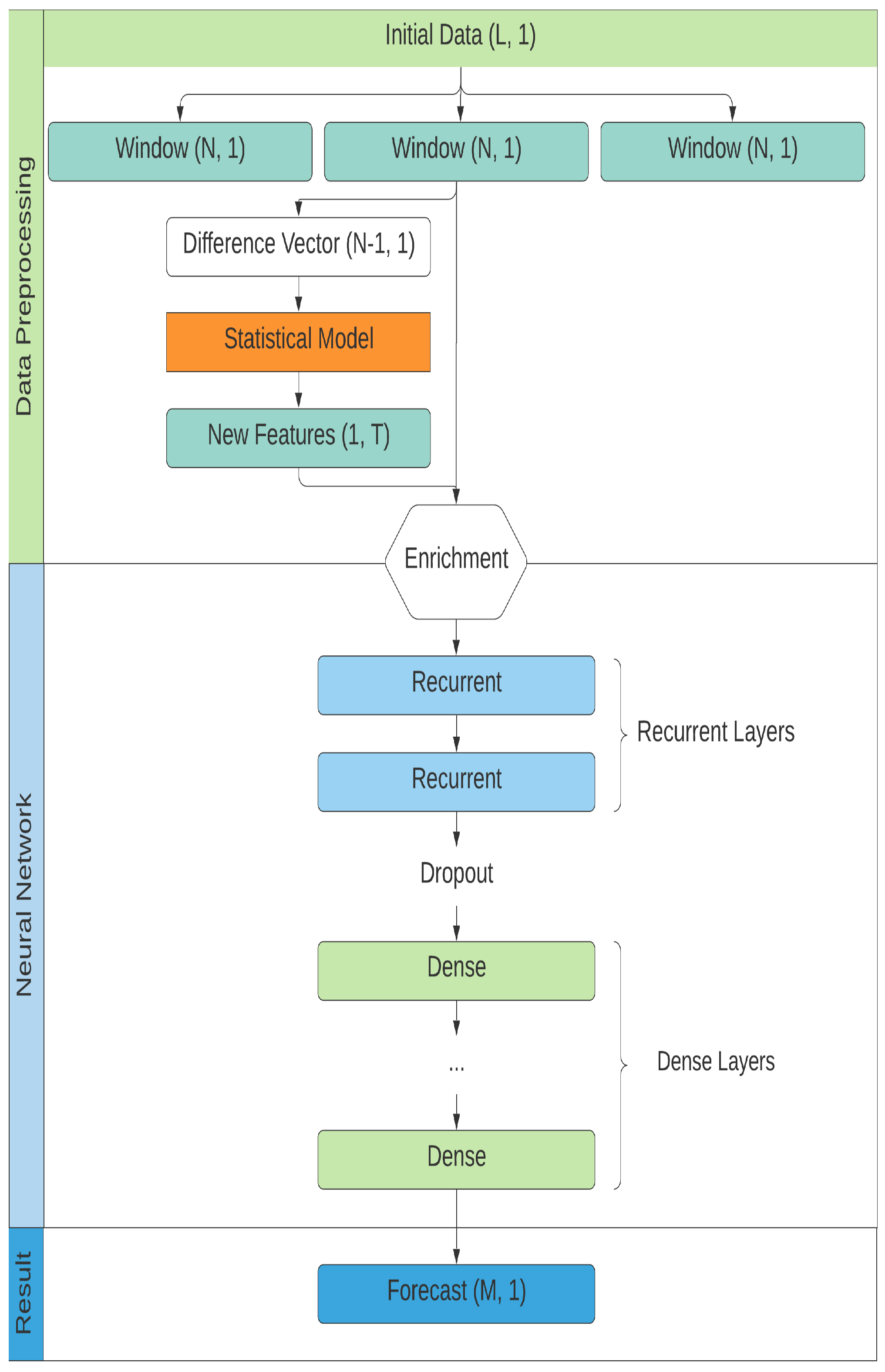
A deep recurrent neural network was created for forecasting. It consists of two recurrent neuron layers followed by several dense layers, see Figure 1.

While the general architecture of the network remained the same, the number of layers and number of neurons in each layer varied depending on the hyperparameter optimization process.

The hyperparameter optimization may improve the performance of neural networks and can be used to adapt commonly used architecture to specific domains [51,52,53]. In this research, the following hyperparameters are varied:

• type of recurrent layers: Long Short-Term Memory (LSTM) [54], recurrent neural network (RNN) [55,56] or Gated Recurrent Units (GRU) [57];
• exact number of dense layers;
• number of neurons in each layer;
• dropout rates [58];
• optimizers for the neural network.

Several recurrent layers were used in a neural network architecture. Deep recurrent neural networks allow for better flexibility compared to one-layer networks and serve as a powerful model for chaotic sequential data. Deep RNN were used for the task of forecasting and achieved better performance compared to shallow recurrent architectures [59,60]. Neural networks of similar architecture were applied to the analysis of indoor navigation [61], climate data [62], human activity classification [63], and health assessment [64]. Achieved results combined with the difference in analyzed data led to the choice of deep RNN architecture. Such combination of deep RNN and MSM algorithms were never used to process climate and physics data prior to this paper.

The enrichment process occurs in-between data processing and neural network construction. We should note that statistical model created on the window $\mathbf{X}$ is a characteristic of that entire window, not a time-dependent characteristic of any specific observation contained in the window. This also applies to the features based on that model.

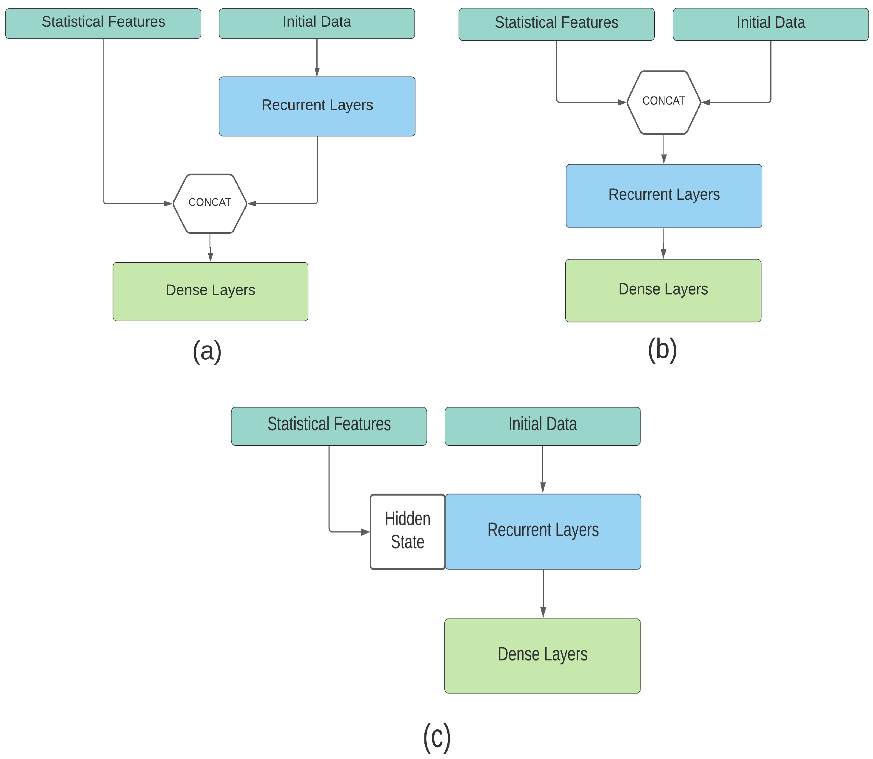
There are several methods of passing features to the neural network. The simplest way to do so is to create a multi-input model by adding statistical features to the data flow after recurrent layers, see Figure 2a. Unfortunately, this also means that those layers would be trained without any information derived from SFC.

In the second approach (see Figure 2b), additional data are added to the window itself. The input vector for neural network consists of original N window observations and additional K SFC features are applied to the end or to the beginning of the data vector. Adding time-independent data to a vector of time observations may create a harder learning task for the neural network. This approach was used but had proven to give worse accuracy compared to the hidden state initialization [65,66].

Finally, the approach presented in Figure 2c directly affects the hidden state of recurrent layers. Additional features for each training sample are transformed into a K-sized vector $\mathbf{v}$ defining the internal state of the recurrent layer:

$$\mathbf{v}=W\mathbf{x}+\mathbf{b},$$

where $\mathbf{x}$ is the vector of features, and W and $\mathbf{b}$ are trainable weights. Those weights can be obtained with an additional single dense layer placed before the recurrent layers of the neural network as a part of the enrichment process. For the first time step, the resulting tensor is added to the hidden state of the RNN. It allows both for conditioning of RNN on additional features and avoiding the problem of increasing the complexity of model training.

3.3. Computational Complexity

Compared to training on non-enriched data, SFC includes an additional step for model creation. We raise a question of computational complexity of the first SFC step compared to the overall complexity of the network training.

The total number of parameters in a LSTM layer can be calculated as follows [67]:

$$W=n_c^2\times 4+n_i\times n_c\times 4+n_c\times n_o+n_o\times 3,$$

where $n_c$ is the number of memory cells, $n_i$ is the number of input units, and $n_o$ is the number of output units. The computational complexity of training the LSTM model per weight and per time step with used optimizers is $O\left(1\right)$. This gives us the computational complexity of $O\left(W\right)$ per time step.

Given the window length N and relatively small prediction size, the computational complexity is dominated by the $n_c\times (n_c+N)$ factor. Finally, given the total time series length of L, the number of windows scales linearly with it. Assuming we have a constraint on maximum number of epochs, we may postulate that the computational complexity of training an LSTM model would be $O(L\times n_c\times (n_c+N))$. Calculations are similar for GRU and RNN layers.

At the same time, the computational complexity of the MSM algorithm, see Algorithm A1, on one window of length N is $O(K\times N)$, where K is the number of components. The main computational complexity lies in the updating of auxiliary matrix g of the algorithm. It gives us the complexity of $O(L\times K\times N)$ for the MSM analysis of the whole time series. This is comparable to the complexity of neural network training. The MSM algorithm can be tailored for operations with matrices leading to a performance improvement on GPU-assisted systems [68].

These results are confirmed by the practical application of SFC in GPU-assisted computing. MSM model construction required significantly less time than model training: the difference reached a factor of ten or even more. Additionally, SFC statistical models on different windows are independent from each other. It means that already computed models could be cached and would not be changed with the addition of new observations to series. This allows for application of SFC to a real-time tasks with continuous data flows.

4. Examples of Real Data Analysis

4.1. Test Data and Neural Networks’ Configurations

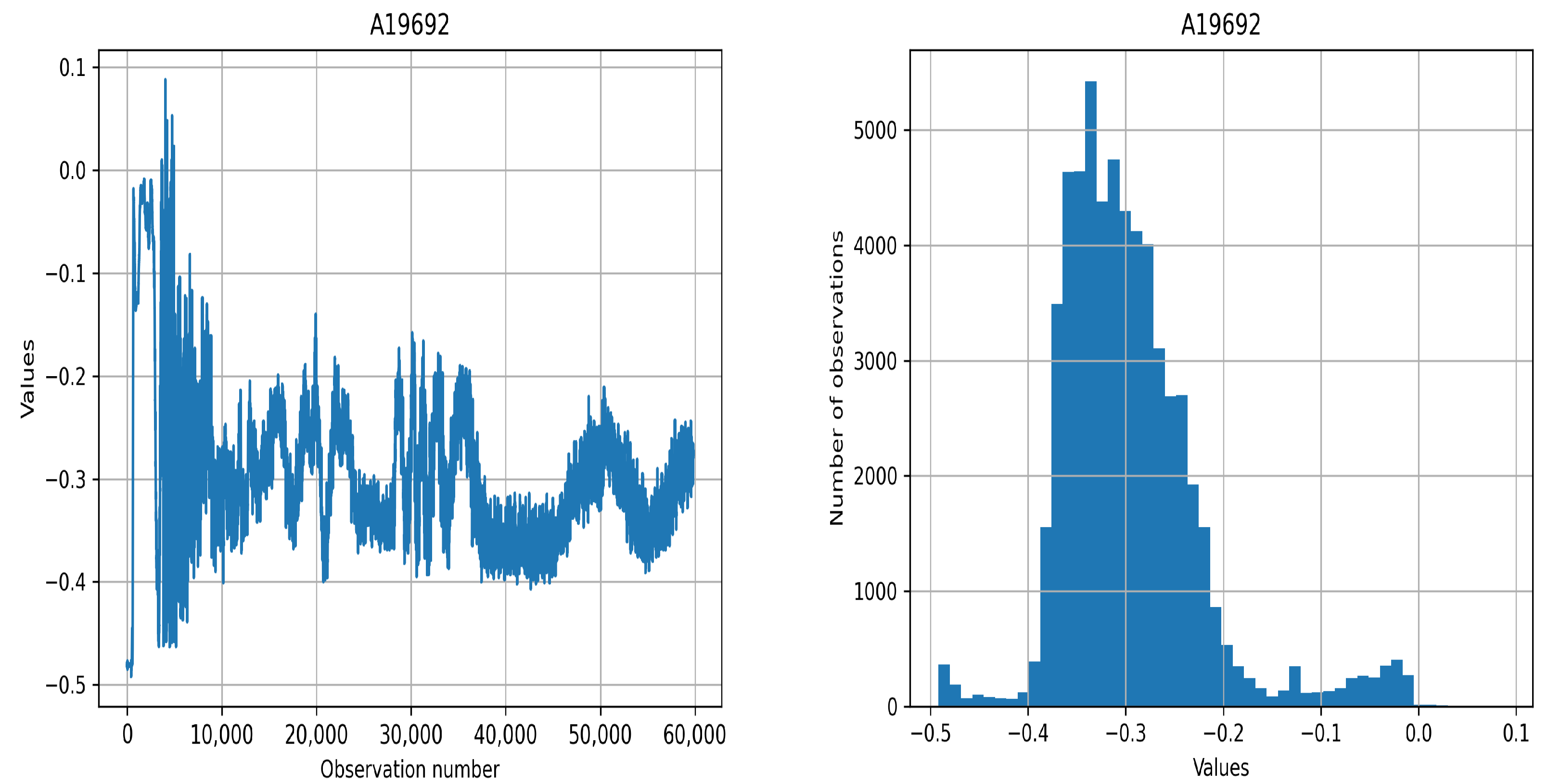
Analyzed datasets consist of two distinct sets. The first set contains data obtained in physical experiments carried on the L-2M stellarator [31]. Time series consists of plasma density fluctuations after the medium had been agitated with an energy discharge. A total of five time series would be analyzed. Each series consists of 60,000 observations that correspond to a time interval from 48 to 60 ms of each experiment. The time gap between two consecutive observations is $0.2$ microsecond ($\mathsf{\mu }$s). Time series from this set had proven to be non-stationary, and the p-value of the Dickey–Fuller test [69] obtains up to $0.56$. For model correctness, it is necessary to analyze not the entire series, but windows, subsamples for which the necessary assumptions are considered to be satisfied, that is, to use the MSM approach. The typical waveform as well as empirical distributions are presented in Figure 3.

The experiment consists of three stages: the initiation stage when the impulse agitates the plasma, the main phase, and the relaxation phase. It is worth noting that the distribution of time series has a strongly non-Gaussian form. It can be seen that an excess of kurtosis and asymmetry exists. It would require complicated models to describe such data.

The second dataset consists of air–sea fluxes [70], see Figure 4.

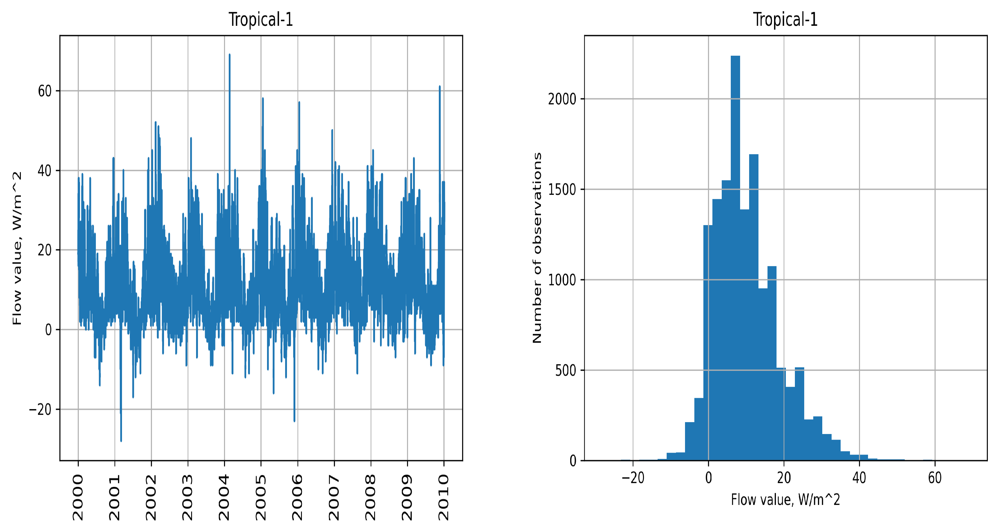
For each spot, two separate time series were collected for latent and hidden fluxes. Each time series consists of approximately $14,600$ observations, and the time gap between two consecutive observations is six hours. Tropical-1 time series and its distribution are shown in Figure 4. These data are highly seasonal in nature, and the distribution is non-Gaussian.

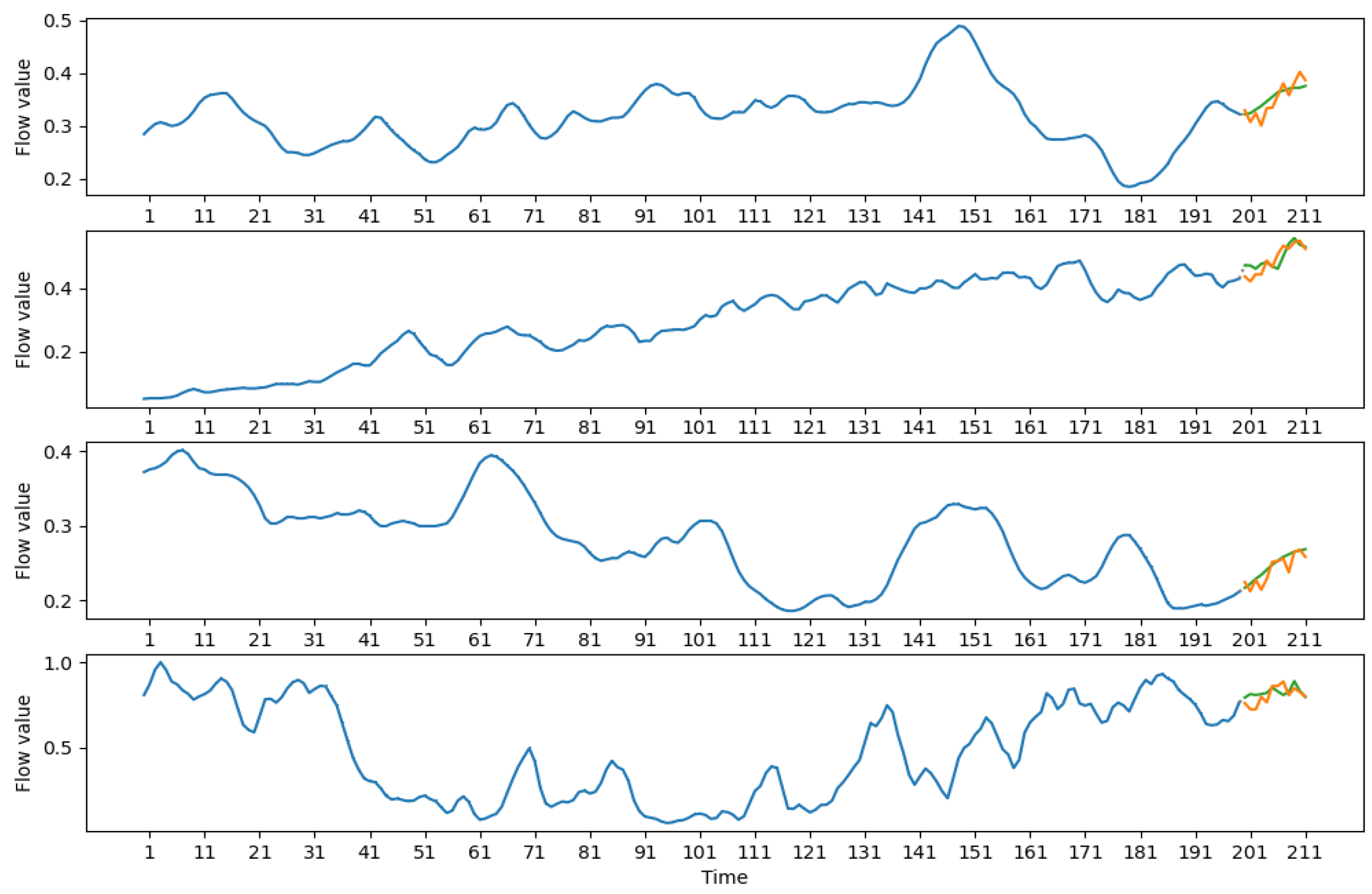
In order to measure the effect of statistical enrichment on the accuracy, two different predictions would be made for each set. Short-term prediction outputs $M=12$ (see Figure 1) consecutive values given the 200 previous values. For oceanographic data, short-term prediction would be a prediction of data for three days after 50 days of observations.

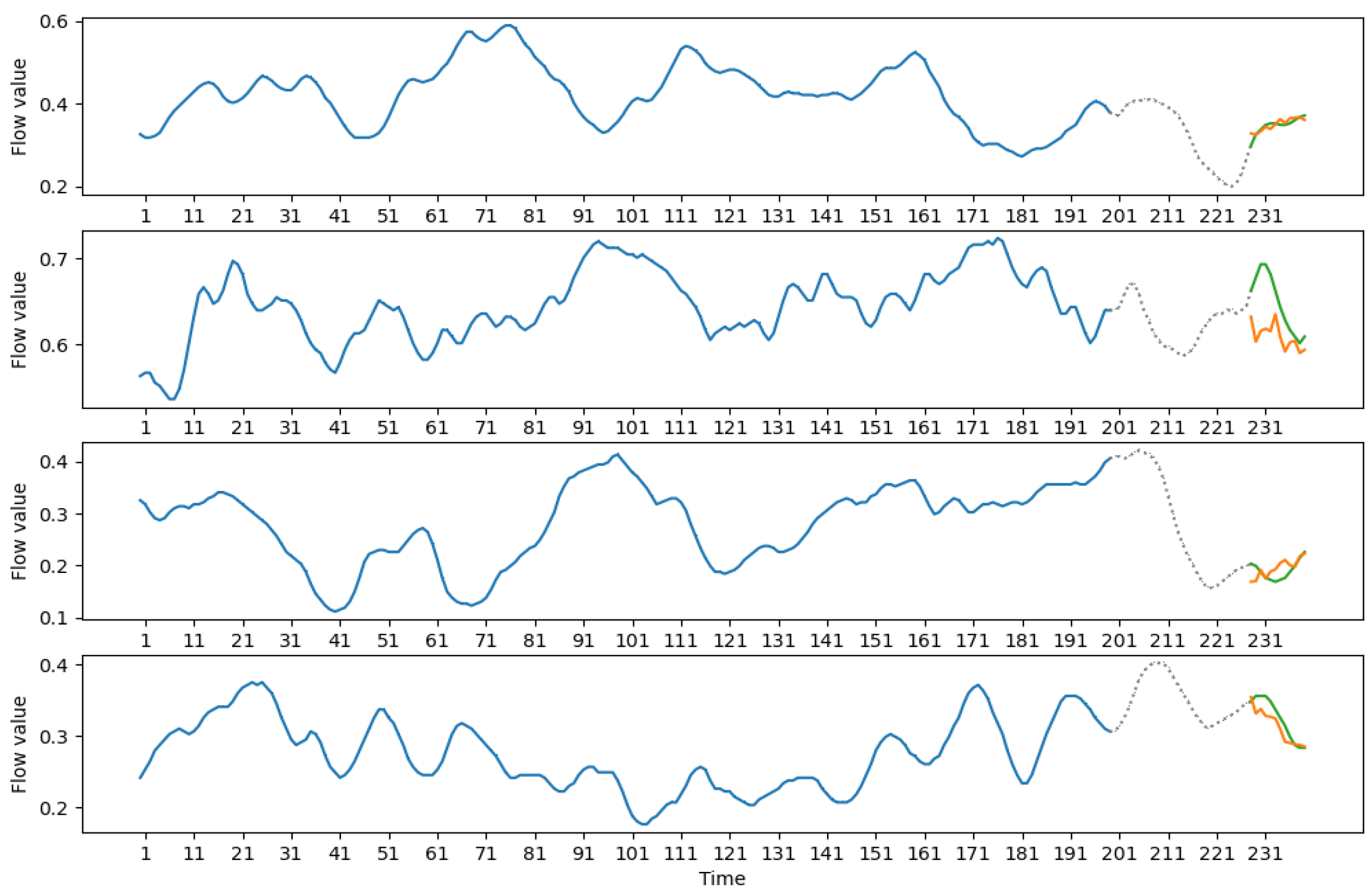
Medium-term prediction outputs $M=12$ consecutive values given the 200 previous values with a skip of 28 observations. Taking the oceanographic data as an example, medium-term prediction would be a prediction of three days on the next week after 50 days of observations.

For the purpose of this research, the size of window $N=200$ (see Figure 1) was chosen to be the same as the size of input data for short- and medium-term predictions. This allows for a proper comparison of enriched and non-enriched accuracy values as no additional data are supplied to the enrichment process if compared to non-enriched data. The number of components $K=3$ was selected for all time series as outlined in Section 3. Based on constructed models, four moments were used as additional statistical features for neural networks.

All data are normalized to the range of $[0,1]$. Error decrease is measured with the root mean squared error metrics over the normalized data forecasts:

$$RMSE=\sqrt{\frac{1}{n}\sum _{i=1}^n{\left(d_i-f_i\right)}^2}.$$

Here, n denotes the number of data points, $d_i$ is the predicted value of i-th data point, and $f_i$ is the true value of the i-th data point. Such approach allows for comparison of the relative error decrease among all analyzed sets of data despite their different physical nature.

In order to demonstrate the efficiency of SFC, two neural network sets were constructed for each time series and prediction type. The original set accepts initial observations as input data. For the enriched network set, time series are supplemented by hidden state initialization with statistical moments. In both cases, the output consists of either a short- or medium-term prediction, in total four sets for each time series.

It is known that random search may provide for better results, but, in order to make a proper comparison of accuracy increase, a grid-search method was used for hyperparameter optimization [30]. Each set contains neural networks with all possible hyperparameter combinations, in total about 700 networks in a set. For each time series, error value is compared between best neural networks in original and enriched short-term sets and between best neural networks in original and enriched medium-term sets.

Input data were divided into training, validation, and test data sets in $60\%/30\%/10\%$ proportion. The customized MSM algorithm and estimation of finite normal mixture parameters were implemented in MATLAB programming language. Neural networks were created, trained, and evaluated with TensorFlow/Keras Python libraries. Every network was ran several times, and the RMSE value was averaged among all runs.

The choice of optimizer varied among observed data sets, but mostly learning speed and accuracy were better with the Adam optimizer. No strong overfitting was observed in all constructed neural networks. A non-zero dropout rate affected learning rate negatively. In all observed cases, the choice of LSTM recurrent layers provided for better results than the use of GRU/RNN layers.

4.2. Results

The calculations were performed using a hybrid high-performance computing cluster (IBM Power 9, 1 TB RAM, 2 NVIDIA Tesla V100 (16 GB) with NVLink). Model training finished after a fixed cut out of 500 epochs or after the error metrics had not decreased for 10 epochs. In practice, training always finished before 500 epochs passed. It took about 20 h to perform a complete hyperparameter search for a single training set. Speed difference between enriched and non-enriched model training varied from $2\%$ to $10\%$ depending on the exact choice of hyperparameters.

Similar best-performing architectures for most analyzed series in both enriched and non-enriched cases were found. As in [16,29], neural networks with a smaller number of wide hidden layers made more accurate predictions than deep neural networks with stacked but narrower hidden layers. The difference in error metrics was significant and reached $35\%$ in certain cases. The choice of optimizer varied among observed data sets. Accuracy and learning speed were mostly better with an Adam optimizer. The non-zero dropout rate affected the learning rate negatively. In all observed cases, the choice of LSTM recurrent layers provided for better results than the use of GRU/RNN layers. In general, the best performance was reached with two dense layers of 300 neurons each, two LSTM layers of 200 neurons each, the Adam optimizer, and no dropout.

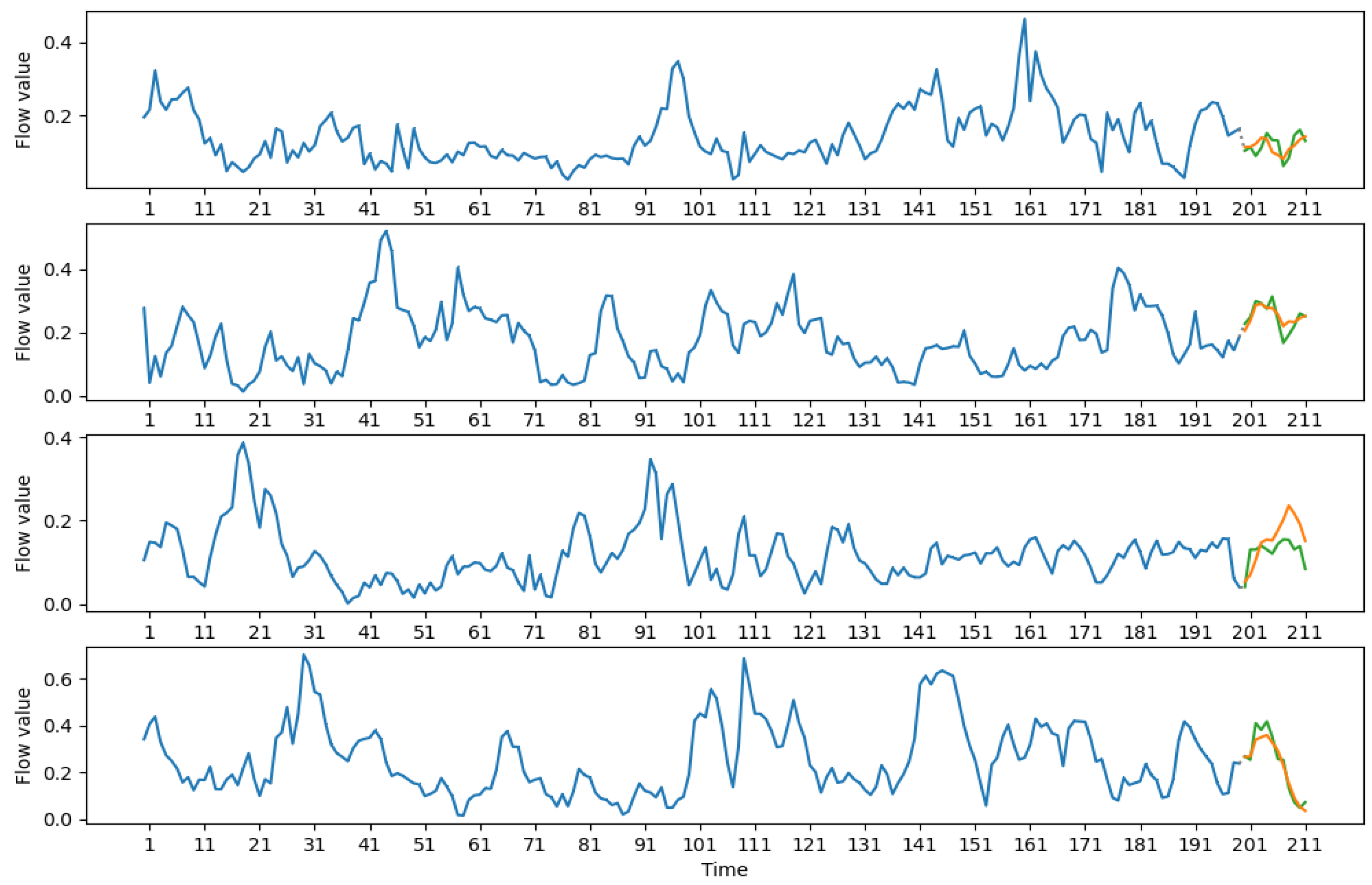
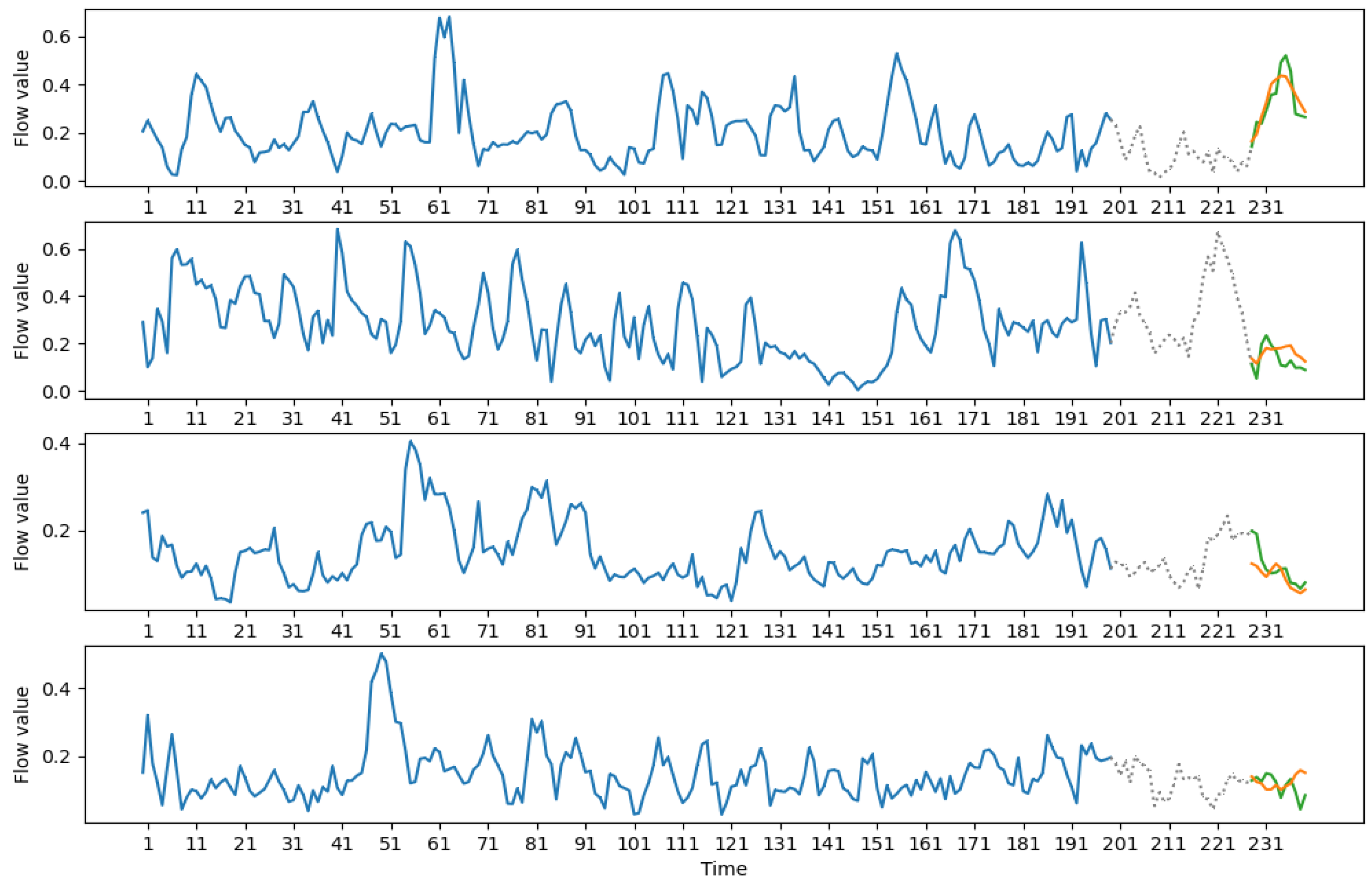
Resulting predictions can be seen in Figure 5, Figure 6, Figure 7 and Figure 8. Each graph denotes several windows and a forecast based on these windows.

The graph of a single forecast consists of three parts: input, designated by a thick blue line; optional skipped data part marked by a dotted line for medium-term forecasts (see Figure 6 and Figure 8) and output designated by orange and green lines. The green line displays the true data, and the orange line is the constructed forecast for the data. Forecasting windows were chosen randomly from the test part of the window series.

It can be seen that the constructed forecasts are good at trend predictions and the direction of overall movement. Peaks are also predicted accurately. It should be noted that, in some cases, the model does not give the accurate forecast of the minimum and maximum values, but, in most observed cases, the minimum of the prediction would lie in a range of 1–2 observations from the true minimum of the forecasted data. The same is true for the maximum.

RMSE results for physical data analysis can be seen in

Table 1. Physical RMSE results, short-term forecast.

Time Series	Non-Enriched	Enriched	Improvements
A19692	$0.085$	$0.061$	$39\%$
A19692-1	$0.086$	$0.061$	$41\%$
A19692-2	$0.095$	$0.094$	$1\%$
A20229	$0.091$	$0.084$	$9\%$
A20264	$0.079$	$0.070$	$12\%$

and 

Table 2. Physical RMSE results, medium-term forecast.

Time Series	Non-Enriched	Enriched	Improvements
A19692	$0.068$	$0.057$	$19\%$
A19692-1	$0.095$	$0.077$	$23\%$
A19692-2	$0.096$	$0.088$	$10\%$
A20229	$0.088$	$0.081$	$8\%$
A20264	$0.078$	$0.071$	$9\%$

. A19692-2 is a clear outlier with almost no decrease of RMSE metric but overall satisfactory forecasts in both the enriched and non-enriched data set. A minor decrease in RMSE metrics is achieved for the short-term forecast, but, for the medium-term forecast, an RMSE decrease of $10\%$ justifies the use of a more complex SFC approach.

Analysis of oceanographic data leads to similar results. RMSE metrics and their improvement are presented in

Table 3. Oceanographic RMSE results, short-term forecast.

Time Series	Non-Enriched	Enriched	Improvements
Gulfstream-1	$0.075$	$0.067$	$11\%$
Gulfstream-2	$0.064$	$0.058$	$11\%$
Labrador-1	$0.069$	$0.060$	$15\%$
Labrador-2	$0.069$	$0.059$	$17\%$
Tropical-1	$0.073$	$0.068$	$7\%$
Tropical-2	$0.074$	$0.061$	$21\%$

and

Table 4. Oceanographic RMSE results, medium-term forecast.

Time Series	Non-Enriched	Enriched	Improvements
Gulfstream-1	$0.081$	$0.075$	$8\%$
Gulfstream-2	$0.072$	$0.066$	$9\%$
Labrador-1	$0.068$	$0.061$	$11\%$
Labrador-2	$0.075$	$0.066$	$14\%$
Tropical-1	$0.073$	$0.072$	$2\%$
Tropical-2	$0.074$	$0.063$	$17\%$

.

The choice between enriched and non-enriched data greatly affected RMSE value for oceanographic data. SFC allowed for 2–$21\%$ decrease in RMSE with an average of $14\%$ for short-term forecasts and $10\%$ for medium-term forecasts. Effective decrease correlated with the analyzed time series. For both types of forecasts, enrichment performed best on Tropical-2 time series and worst on Tropical-1 time series.

This level of accuracy improvement according to the RMSE metric may be due to the fact that, for a specific set of Tropical-1, the basic neural network model already provides a complete description of the analyzed processes. Therefore, the feature space expansion provides only to a marginal decrease of learning error. In all other situations, the SFC based decrease is very noticeable, so such a series can be considered as an outlier for the proposed method. At the same time, it should be noted that there is still no error increase for Tropical-1. It means that the proposed method is effective in all situations, but the magnitude of its effect may vary.

It should be noted that there was no increase of RMSE error observed among all enriched sets when compared to the original. For all sets, short-term and medium-term forecasts follow major data trends. At the same time, enriched sets produce forecasts that are better at adapting to quick shifts in data. Additionally enriched forecasts offer better prediction of peak values compared to non-enriched data.

5. Discussion and Conclusions

The paper presents a statistical approach to data modeling and feature construction with applications for two different sets of data. For six oceanographic datasets and five plasma physics datasets, multiple neural networks were constructed and trained in an enriched and non-enriched form. For all analyzed time series, a qualitative predictions were created for both methods with an average RMSE error of $0.068/0.078$ for short-term forecasts and $0.071/0.079$ for medium-term forecasts.

From the numerical perspective, statistical feature construction had shown a significant decrease in RMSE error metrics among all analyzed time series. The decrease ranged from $1\%$ to $43\%$ with the median of $11.4\%$ and happened on all analyzed time series. It was also shown that SFC does not add significant computational complexity to the process of forecasting and can be used with continuous data flows and/or in real-time problems. This method can also be adjusted for GPU computing.

The significance of the work lies in the possibility of accuracy improvement with a relatively simple addition to preliminary data analysis. SFC does not require additional data collection and, as shown above, can be applied to a wide range of different problems where a stochastic external environment presents. The first step of SFC has relatively few hyperparameters for optimization, which leads to a smaller overhead on their optimization. Lastly, the increase of forecasting accuracy due to SFC application can serve as an indicator of correctness of the chosen statistical model.

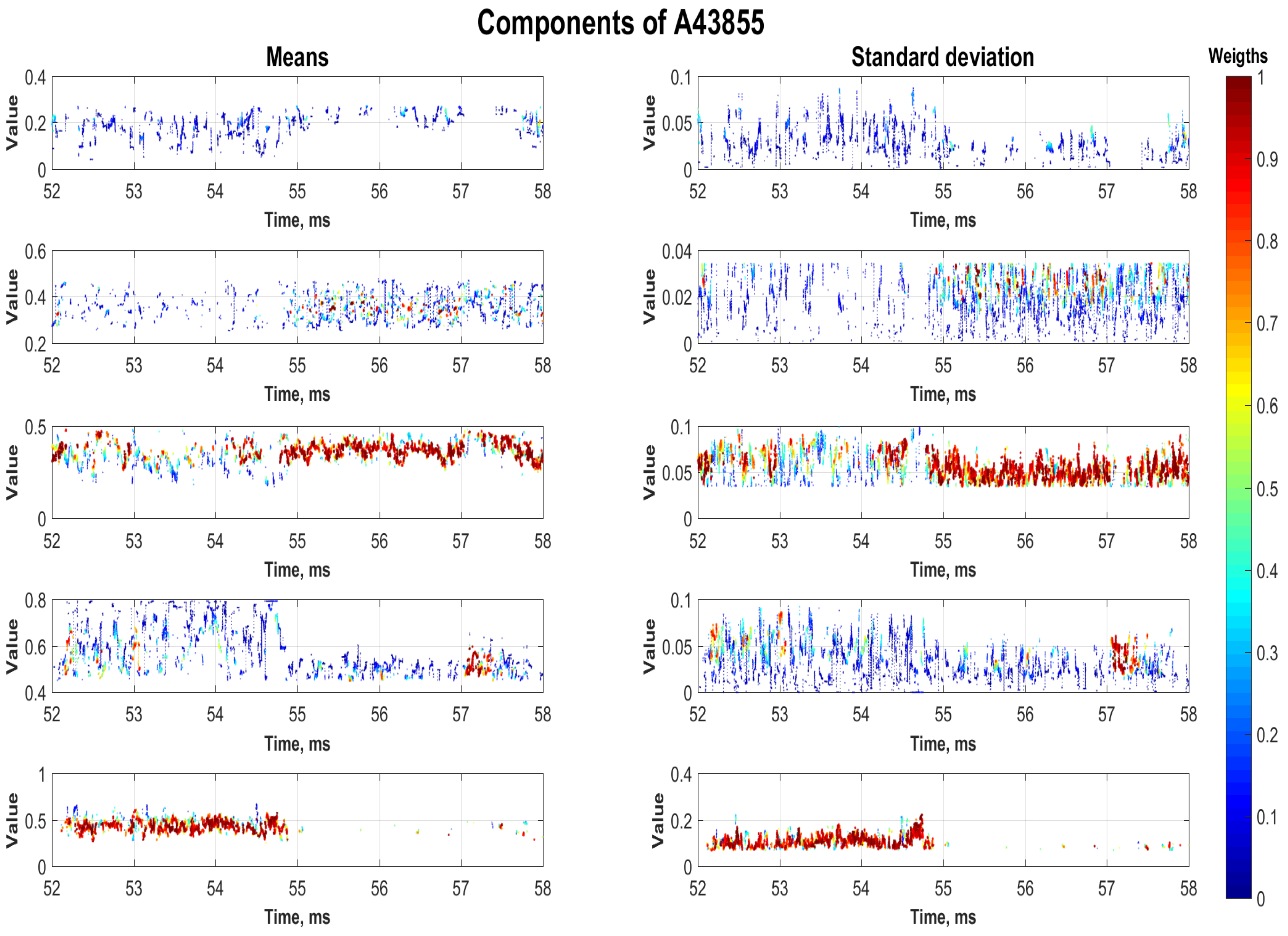
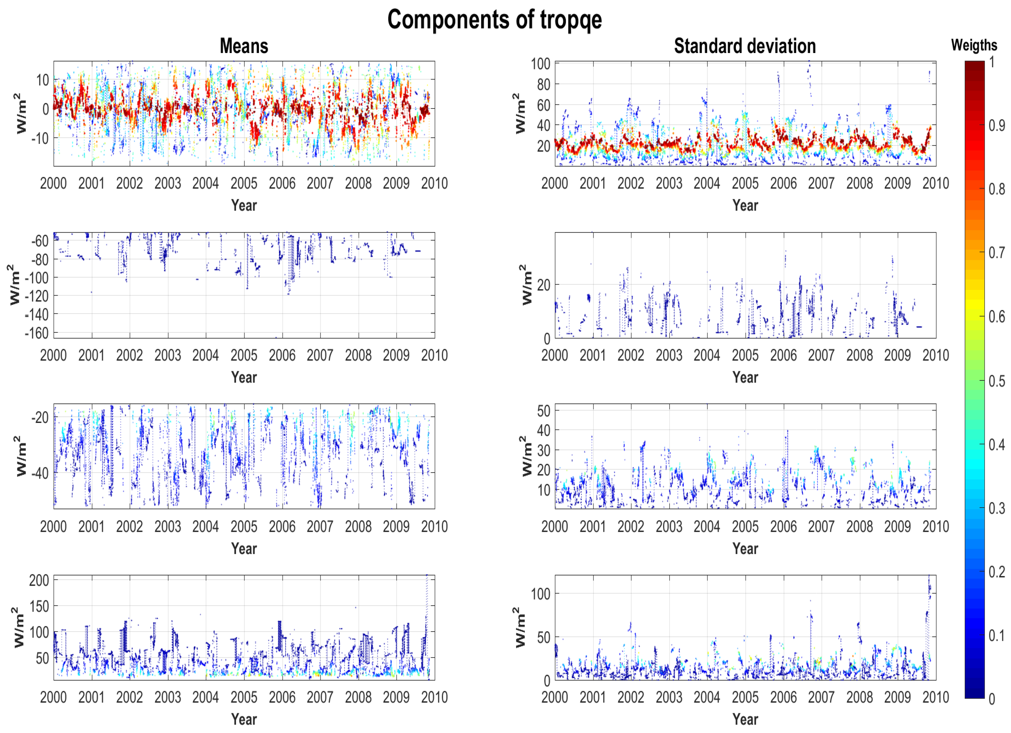
For future research, it would be beneficial to apply another features from MSM models to forecast improvement. For example, in Figure 9 and Figure 10, an evolution of MSM components [71] is demonstrated. These structural components do not correspond to the summands in formula (1) but are derived from them with the help of clustering algorithms. The colors signify the corresponding weight of the component in the mixture (1).

The MSM components based method allows us to determine significant changes in the stochastic structure of the forming processes. In particular, the detection of the time moment of an essential change in plasma parameters, which affects its confinement (the so-called transport transition), has been demonstrated, see Figure 9. Component number 5 with the maximum weight (red curve in the lower graphs in Figure 9) has the greatest contribution to the process. However, it breaks off at about 55 ms of the experiment and, after that, component number 3 dominates.

A similar situation takes place for oceanographic time series, see Figure 10. Here, a smaller number of structural components are distinguished, and no abrupt disappearances or creation of new components are observed.

Other finite mixture models that have more features than a normal distribution could be employed. Those may include finite mixtures based on skew-normal or skew-t densities [12]. MSM components can be effectively used to process non-trivial trends in data, which would make it possible to better predict complex time series using neural networks. Surely, this will require sophisticated architectures such as ensembles of deep LSTM networks. However, such solutions are a natural development of the SFC approach proposed in this article.

References

- Korolev, V.Y. Probabilistic and Statistical Methods of Decomposition of Volatility of Chaotic Processes; Izd-vo Moskovskogo un-ta: Moscow, Russia, 2011. [Google Scholar]
- Korolev, V.Y. Convergence of random sequences with independent random indexes I. Theory Probab. Its Appl. 1994, 39, 313–333. [Google Scholar] [CrossRef]
- Korolev, V.Y. Convergence of random sequences with independent random indexes II. Theory Probab. Appl. 1995, 40, 770–772. [Google Scholar] [CrossRef]
- Korolev, V.Y.; Gorshenin, A.K. Probability models and statistical tests for extreme precipitation based on generalized negative binomial distributions. Mathematics 2020, 8, 604. [Google Scholar] [CrossRef] [Green Version]
- Gorshenin, A.K.; Korolev, V.Y.; Zeifman, A.I. Modeling particle size distribution in lunar regolith via a central limit theorem for random sums. Mathematics 2020, 8, 1409. [Google Scholar] [CrossRef]
- Audhkhasi, K.; Osoba, O.; Kosko, B. Noise-enhanced convolutional neural networks. Neural Netw. 2016, 78, 15–23. [Google Scholar] [CrossRef] [PubMed]
- McLachlan, G.; Peel, D. Finite Mixture Models; John Wiley & Sons: New York, NY, USA, 2000. [Google Scholar]
- Gorshenin, A.; Korolev, V. Modelling of statistical fluctuations of information flows by mixtures of gamma distributions. In Proceedings of the 27th European Conference on Modelling and Simulation, Alesund, Norway, 27–30 May 2013; Digitaldruck Pirrot GmbHP: Dudweiler, Germany, 2013; pp. 569–572. [Google Scholar]
- Liu, C.; Li, H.-C.; Fu, K.; Zhang, F.; Datcu, M.; Emery, W.J. A robust EM clustering algorithm for Gaussian mixture models. Pattern Recognit. 2019, 87, 269–284. [Google Scholar] [CrossRef]
- Wu, D.; Ma, J. An effective EM algorithm for mixtures of Gaussian processes via the MCMC sampling and approximation. Neurocomputing 2019, 331, 366–374. [Google Scholar] [CrossRef]
- Zeller, C.B.; Cabral, C.R.B.; Lachos, V.H.; Benites, L. Finite mixture of regression models for censored data based on scale mixtures of normal distributions. Adv. Data Anal. Classif. 2019, 13, 89–116. [Google Scholar] [CrossRef]
- Abid, S.H.; Quaez, U.J.; Contreras-Reyes, J.E. An information-theoretic approach for multivariate skew-t distributions and applications. Mathematics 2021, 9, 146. [Google Scholar] [CrossRef]
- Greff, K.; van Steenkiste, S.; Schmidhuber, J. Neural expectation maximization. In Proceedings of the 31st International Conference on Neural Information Processing Systems, Long Beach, CA, USA, 4–9 December 2017; MIT Press: Cambridge, MA, USA, 2017; pp. 6694–6704. [Google Scholar]
- Viroli, C.; McLachlan, G.J. Deep Gaussian mixture models. Stat. Comput. 2019, 29, 43–51. [Google Scholar] [CrossRef] [Green Version]
- Alawe, I.; Ksentini, A.; Hadjadj-Aoul, Y.; Bertin, P. Improving traffic forecasting for 5G core network scalability: A machine learning approach. IEEE Netw. 2018, 32.6, 42–49. [Google Scholar] [CrossRef] [Green Version]
- Gorshenin, A.K.; Kuzmin, V.Y. Neural network forecasting of precipitation volumes using patterns. Pattern Recognit. Image Anal. Adv. Math. Theory Appl. 2018, 28, 450–461. [Google Scholar] [CrossRef]
- Weyn, J.A.; Durran, D.R.; Caruana, R. Improving data-driven global weather prediction using deep convolutional neural networks on a cubed sphere. J. Adv. Model. Earth Syst. 2020, 12, e2020MS002109. [Google Scholar] [CrossRef]
- Chandrashekar, G.; Sahin, F. A survey on feature selection methods. Comput. Electr. Eng. 2014, 40. 1, 16–28. [Google Scholar] [CrossRef]
- Bennasar, M.; Hicks, Y.; Setchi, R. Feature selection using Joint Mutual Information Maximisation. Expert Syst. Appl. 2015, 42, 8520–8532. [Google Scholar] [CrossRef] [Green Version]
- Jovic, A.; Brkic, K.; Bogunovic, N. A review of feature selection methods with applications. In Proceedings of the 38th International Convention on Information and Communication Technology, Electronics and Microelectronics (MIPRO), Opatija, Croatia, 25–29 May 2015; Biljanovic, P., Butkovic, Z., Skala, K., Mikac, B., Cicin-Sain, M., Sruk, V., Ribaric, S., Gros, S., Vrdoljak, B., Mauher, M., Eds.; IEEE: Manhattan, NY, USA, 2015; pp. 1200–1205. [Google Scholar]
- Xue, B.; Zhang, M.J.; Browne, W.N.; Yao, X. A Survey on Evolutionary Computation Approaches to Feature Selection. IEEE Trans. Evol. Comput. 2016, 20, 606–626. [Google Scholar] [CrossRef] [Green Version]
- Sheikhpour, R.; Sarram, M.A.; Gharaghani, S.; Chahooki, M.A.Z. A Survey on semi-supervised feature selection methods. Pattern Recognit. 2017, 64, 141–158. [Google Scholar] [CrossRef]
- Abualigah, L.M.; Khader, A.T.; Hanandeh, E.S. A new feature selection method to improve the document clustering using particle swarm optimization algorithm. J. Comput. Sci. 2018, 25, 456–466. [Google Scholar] [CrossRef]
- Cai, J.; Luo, J.W.; Wang, S.L.; Yang, S. Feature selection in machine learning: A new perspective. Neurocomputing 2018, 300, 70–79. [Google Scholar] [CrossRef]
- Li, J.D.; Cheng, K.W.; Wang, S.H.; Morstatter, F.; Trevino, R.P.; Tang, J.L.; Liu, H. Feature Selection: A Data Perspective. ACM Comput. Surv. 2018, 50, 94. [Google Scholar] [CrossRef] [Green Version]
- Gopika, N.; ME, A.M.K. Correlation based feature selection algorithm for machine learning. In Proceedings of the 3rd International Conference on Communication and Electronics Systems (ICCES), Coimbatore, Tamil Nadu, India, 15–16 October 2018; IEEE Computer Society Press: Piscataway, NJ, USA, 2018; pp. 692–695. [Google Scholar]
- Lee, C.Y.; Shen, Y.X. Optimal feature selection for power-quality disturbances classification. IEEE Trans. Power Deliv. 2011, 26, 2342–2351. [Google Scholar] [CrossRef]
- Wu, Y.; Xu, Y.; Li, J. Feature construction for fraudulent credit card cash-out detection. Decis. Support Syst. 2019, 127, 113155. [Google Scholar] [CrossRef]
- Gorshenin, A.K.; Kuzmin, V.Y. Method for improving accuracy of neural network forecasts based on probability mixture models and its implementation as a digital service. Inform. Primen. 2021, 15, 63–74. [Google Scholar]
- Gorshenin, A.K.; Kuzmin, V.Y. Improved architecture and configurations of feedforward neural networks to increase accuracy of predictions for moments of finite normal mixtures. Pattern Recognit. Image Anal. 2019, 29, 79–88. [Google Scholar] [CrossRef]
- Batanov, G.M.; Berezhetskii, M.S.; Borzosekov, V.D.; Vasilkov, D.G.; Vafin, I.Y.; Grebenshchikov, S.E.; Grishina, I.A.; Kolik, L.V.; Konchekov, E.M.; Shchepetov, S.V.; et al. Reaction of turbulence at the edge and in the center of the plasma column to pulsed impurity injection caused by the sputtering of the wall coating in L-2M stellarator. Plasma Phys. Rep. 2017, 43, 818–823. [Google Scholar] [CrossRef]
- Korolev, V.Y.; Gorshenin, A.K.; Gulev, S.K.; Belyaev, K.P. Statistical modeling of air–sea turbulent heat fluxes by finite mixtures of Gaussian distributions ITMM’2015 Commun. Comput. Inf. Sci. 2015, 564, 152–162. [Google Scholar]
- Batanov, G.M.; Borzosekov, V.D.; Gorshenin, A.K.; Kharchev, N.K.; Korolev, V.Y.; Sarskyan, K.A. Evolution of statistical properties of microturbulence during transient process under electron cyclotron resonance heating of the L-2M stellarator plasma. Plasma Phys. Control. Fusion 2019, 61, 075006. [Google Scholar] [CrossRef]
- Meneghini, O.; Luna, C.J.; Smith, S.P.; Lao, L.L. Modeling of transport phenomena in tokamak plasmas with neural networks. Phys. Plasmas 2014, 21, 060702. [Google Scholar] [CrossRef]
- Raja, M.A.Z.; Shah, F.H.; Tariq, M.; Ahmad, I.; Ahmad, S.U. Design of artificial neural network models optimized with sequential quadratic programming to study the dynamics of nonlinear Troesch’s problem arising in plasma physics. Neural Comput. Appl. 2018, 29, 83–109. [Google Scholar] [CrossRef]
- Wei, Y.; Levesque, J.P.; Hansen, C.J.; Mauel, M.E.; Navratil, G.A. A dimensionality reduction algorithm for mapping tokamak operational regimes using a variational autoencoder (VAE) neural network. Nucl. Fusion 2021, 61, 126063. [Google Scholar] [CrossRef]
- Mesbah, A.; Graves, D.B. Machine learning for modeling, diagnostics, and control of non-equilibrium plasmas. J. Phys. Appl. Phys. 2019, 52, 30LT02. [Google Scholar] [CrossRef] [Green Version]
- Narita, E.; Honda, M.; Nakata, M.; Yoshida, M.; Hayashi, N.; Takenaga, H. Neural-network-based semi-empirical turbulent particle transport modelling founded on gyrokinetic analyses of JT-60U plasmas. Nucl. Fusion 2019, 59, 106018. [Google Scholar] [CrossRef]
- Parsons, M.S. Interpretation of machine-learning-based disruption models for plasma control. Plasma Phys. Control. Fusion 2017, 59, 085001. [Google Scholar] [CrossRef]
- Kates-Harbeck, J.; Svyatkovskiy, A.; Tang, W. Predicting disruptive instabilities in controlled fusion plasmas through deep learning. Nature 2019, 568, 526–531. [Google Scholar] [CrossRef] [PubMed]
- Aymar, R.; Barabaschi, P.; Shimomura, Y. The ITER design. Plasma Phys. Control. Fusion 2002, 44, 519–565. [Google Scholar] [CrossRef]
- Teicher, H. Identifiability of mixtures. Ann. Math. Stat. 1961, 32, 244–248. [Google Scholar] [CrossRef]
- Teicher, H. Identifiability of Finite Mixtures. Ann. Math. Stat. 1963, 34, 1265–1269. [Google Scholar] [CrossRef]
- Gorshenin, A.K. Concept of online service for stochastic modeling of real processes. Inform. Primen. 2016, 10, 72–81. [Google Scholar]
- Gorshenin, A.K. On some mathematical and programming methods for construction of structural models of information flows. Inform. Primen. 2017, 11, 58–68. [Google Scholar]
- Gorshenin, A.K.; Kuzmin, V.Y. Research support system for stochastic data processing. Pattern Recognit. Image Anal. 2017, 27, 518–524. [Google Scholar] [CrossRef]
- Akaike, H. Information theory and an extension of the maximum likelihood principle. In Proceedings of the 2nd International Symposium on Information Theory, Tsahkadsor, Armenia, USSR, 2–8 September 1971; Petrov, B.N., Csáki, F., Eds.; Akadémiai Kiadó: Budapest, Hungary, 1973; pp. 267–281. [Google Scholar]
- Schwarz, G.E. Estimating the dimension of a model. Ann. Stat. 1978, 6, 461–464. [Google Scholar] [CrossRef]
- Gorshenin, A.; Kuzmin, V. Online system for the construction of structural models of information flows. In Proceedings of the 7th International Congress on Ultra Modern Telecommunications and Control Systems and Workshops (ICUMT), Brno, Czech Republic, 6–8 October 2015; IEEE Computer Society Press: Piscataway, NJ, USA, 2015; pp. 216–219. [Google Scholar]
- Gorshenin, A.K.; Kuzmin, V.Y. On an interface of the online system for a stochastic analysis of the varied information flows. AIP Conf. Proc. 2016, 1738, 220009. [Google Scholar]
- Kohavi, R.; John, G. Automatic Parameter Selection by Minimizing Estimated Error. In Proceedings of the Twelfth International Conference on Machine Learning, Tahoe City, CA, USA, 9–12 July 1995; Prieditis, A., Russell, S., Eds.; Morgan Kaufmann Publishers: Burlington, MA, USA, 1995; pp. 304–312. [Google Scholar]
- Sanders, S.; Giraud-Carrier, C. Informing the Use of Hyperparameter Optimization Through Metalearning. In Proceedings of the 2017 IEEE International Conference on Big Data, Boston, MA, USA, 11–14 December 2017; Gottumukkala, R., Ning, X., Dong, G., Raghavan, V., Aluru, S., Karypis, G., Miele, L., Wu, X., Eds.; IEEE Computer Society Press: Piscataway, NJ, USA, 2017; pp. 1051–1056. [Google Scholar]
- Bergstra, J.; Bengio, Y. Random Search for Hyper-Parameter Optimization. J. Mach. Learn. Res. 2012, 13, 281–305. [Google Scholar]
- Greff, K.; Srivastava, R.K.; Koutnik, J.; Steunebrink, B.R.; Schmidhuber, J. LSTM: A Search Space Odyssey. IEEE Trans. Neural Networks Learn. Syst. 2017, 28, 2222–2232. [Google Scholar] [CrossRef] [Green Version]
- Williams, J.; Hinton, E.; Rumelhart, E. Learning representations by back-propagating errors. Nature 1986, 323, 533–536. [Google Scholar] [CrossRef]
- Buduma, N. Fundamentals of Deep Learning: Designing Next-Generation Machine Intelligence Algorithms; O’Reilly Media: Sebastopol, CA, USA, 2017. [Google Scholar]
- Cho, K.; van Merrienboer, B.; Gulcehre, C.; Bahdanau, D.; Bougares, F.; Schwenk, H.; Bengio, Y. Learning Phrase Representations using RNN Encoder-Decoder for Statistical Machine Translation. In Proceedings of the 2014 Conference on Empirical Methods in Natural Language Processing, EMNLP, Doha, Qatar, 25–29 October 2014; Moschitti, A., Pang, B., Daelemans, W., Eds.; Association for Computational Linguistics: Stroudsburg, PA, USA, 2014; pp. 1724–1734. [Google Scholar]
- Srivastava, N.; Hinton, G.; Krizhevsky, A.; Sutskever, I.; Salakhutdinov, R. Dropout: A Simple Way to Prevent Neural Networks from Overfitting. J. Mach. Learn. Res. 2014, 15, 1929–1958. [Google Scholar]
- Sagheer, A.; Kotb, M. Time series forecasting of petroleum production using deep LSTM recurrent networks. Neurocomputing 2019, 323, 203–213. [Google Scholar] [CrossRef]
- Sagheer, A.; Kotb, M. Unsupervised Pre-training of a Deep LSTM-based Stacked Autoencoder for Multivariate Time Series Forecasting Problems. Sci. Rep. 2019, 9, 19038. [Google Scholar] [CrossRef] [Green Version]
- Chen, Z.; Zou, H.; Yang, J.; Jiang, H.; Xie, L. WiFi Fingerprinting Indoor Localization Using Local Feature-Based Deep LSTM. IEEE Syst. J. 2020, 14, 3001–3010. [Google Scholar] [CrossRef]
- Majhi, B.; Naidu, D.; Mishra, A.P.; Satapathy, S.C. Improved prediction of daily pan evaporation using Deep-LSTM model. Neural Comput. Appl. 2020, 32, 7823–7838. [Google Scholar] [CrossRef]
- Eyobu, O.S.; Han, D.S. Feature Representation and Data Augmentation for Human Activity Classification Based on Wearable IMU Sensor Data Using a Deep LSTM Neural Network. Sensors 2018, 18, 2892. [Google Scholar] [CrossRef] [Green Version]
- Miao, H.; Li, B.; Sun, C.; Liu, J. Joint Learning of Degradation Assessment and RUL Prediction for Aeroengines via Dual-Task Deep LSTM Networks. IEEE Trans. Ind. Inform. 2019, 15, 5023–5032. [Google Scholar] [CrossRef]
- Karpathy, A.; Joulin, A.; Fei-Fei, L. Deep fragment embeddings for bidirectional image sentence mapping. In Proceedings of the 27th International Conference on Neural Information Processing Systems, Montreal, QC, Canada, 8–13 December 2014; MIT Press: Cambridge, MA, USA, 2014; Volume 2, pp. 1889–1897. [Google Scholar]
- Karpathy, A.; Fei-Fei, L. Deep visual-semantic alignments for generating image descriptions. In Proceedings of the IEEE Conference on Computer Vision and Pattern Recognition, Boston, MA, USA, 7–12 June 2015; IEEE Computer Society Press: Piscataway, NJ, USA; pp. 3128–3137. [Google Scholar]
- Sak, H.; Senior, A.; Beaufays, F. Long short-term memory based recurrent neural network architectures for large vocabulary speech recognition. arXiv 2014, arXiv:1402.1128. [Google Scholar]
- Gorshenin, A.K. On Implementation of EM-type Algorithms in the Stochastic Models for a Matrix Computing on GPU. AIP Conf. Proc. 2015, 1648, 250008. [Google Scholar]
- Dickey, D.A.; Fuller, W.A. Distribution of the Estimators for Autoregressive Time Series with a Unit Root. J. Am. Stat. Assoc. 1979, 74, 427–431. [Google Scholar]
- Perry, A.H.; Walker, J.M. The Ocean Atmosphere System; Longman: New York, NY, USA, 1977. [Google Scholar]
- Gorshenin, A.K.; Korolev, V.Y.; Shcherbinina, A.A. Statistical estimation of distributions of random coefficients in the Langevin stochastic differential equation. Inform. Primen. 2020, 14, 3–12. [Google Scholar]
Figure 1.
Architecture of SFC processing with a neural network.
Figure 2.
Methods of passing features to the neural network: (a) multi-input model; (b) adding features to window; (c) hidden state initialization.
Figure 3.
Physical time series A19692 (on the left) a corresponding histogram (on the right).
Figure 4.
Tropical-1 time series (on the left) a corresponding histogram (on the right).
Figure 5.
A19692 short-term forecasts.
Figure 6.
A19692-1 medium-term forecasts.
Figure 7.
Gulfstream-1 short-term forecasts.
Figure 8.
Gulfstream-1 medium-term forecasts.
Figure 9.
Example of MSM components for plasma time series.
Figure 10.
Example of MSM components for oceanographic time series.