Dynamic Multicriteria Games with Finite Horizon


1
Institute of Applied Mathematical Research of the Karelian Research Centre of RAS, 11, Pushkinskaya Str., Petrozavodsk 185910, Russia
2
Saint-Petersburg State University, 7–9, Universitetskaya Nab., Saint-Petersburg 199034, Russia
†
Current address: 11, Pushkinskaya str., Petrozavodsk 185910, Russia.
Mathematics 2018, 6(9), 156; https://doi.org/10.3390/math6090156
Submission received: 31 July 2018
/
Revised: 8 August 2018
/
Accepted: 3 September 2018
/
Published: 5 September 2018
(This article belongs to the Special Issue Mathematical Game Theory)
Abstract
:The approaches to construct optimal behavior in dynamic multicriteria games with finite horizon are presented. To obtain a multicriteria Nash equilibrium, the bargaining construction (Nash product) is adopted. To construct a multicriteria cooperative equilibrium, a Nash bargaining scheme is applied. Dynamic multicriteria bioresource management problem with finite harvesting times is considered. The players’ strategies and the payoffs are obtained under cooperative and noncooperative behavior.
MSC:
22E461. Introduction
Mathematical models involving more than one objective seem more adherent to real problems. Players can have more than one goal which are often not comparable. These situations are typical for game-theoretic models in economy and ecology. For example, in management problems the decision maker wants to maximize her profit and to minimize the production costs, in bioresource management problems the players wish to maximize their exploitation rates and to minimize the harm to the environment, and so on. Hence, a multicriteria game approach helps to make decisions in multi-objective problems.
Traditionally, equilibrium analysis in multicriteria problems is based on the static variant. Some concepts have been suggested to solve multicriteria games (e.g., the ideal Nash equilibrium [1], the E-equilibrium concept [2]). However the notion of Pareto equilibrium is the most-studied concept in multicriteria game theory.
This paper is dedicated to optimal behavior design in dynamic multicriteria games with finite horizon. To construct noncooperative equilibrium, we adopt the approach in [3]. The multicriteria Nash equilibrium is obtained by applying the bargaining concept (via Nash products), with the guaranteed payoffs playing the role of the status quo points. To determine the cooperative equilibrium in dynamic games with many objectives, we adopt the Nash bargaining scheme. Namely, the cooperative strategies and payoffs are constructed via a Nash bargaining solution, with the multicriteria Nash equilibrium payoffs playing the role of the status quo points.
Further exposition has the following structure. Classical solution concepts for noncooperative and cooperative multicriteria games are given in Section 2. Section 3 describes the proposed noncooperative and cooperative solution concepts for a finite horizon multicriteria dynamic game with two participants in discrete time. A two-player discrete-time game-theoretic bioresource management model (harvesting problem) with a finite planning horizon is treated in Section 4. The noncooperative behavior is obtained in Section 4.1, whereas the cooperative case is treated in Section 4.2. Finally, Section 5 provides the basic results and their discussion.
2. Multicriteria Games and Solution Concepts
A multicriteria noncooperative game is
where gives the set of players, is the set of strategies of player i, and denotes the payoff function of player i, , .
Shapley [4] gave a generalization of the classical Nash equilibrium to Pareto equilibrium for such games.
Definition 1.
A strategy profile is a
- 1.
- weak Pareto equilibrium if
- 2.
- strong Pareto equilibrium if
Here , , .
Other solution concepts for multicriteria games, namely ideal Nash equilibrium and E-equilibrium, were introduced in [1,2], respectively. Reference [5] connected multicriteria games with potential games, and the coalition formation processes for multicriteria games were considered in [6].
A multicriteria cooperative game is defined as
where is the set of players, denotes the characteristic function, , and
For cooperative multicriteria games, the natural generalization of the Shapley value is applied to distribute the cooperative payoff among the players.
Definition 2.
The Shapley value of the multicriteria game is
3. Dynamic Multicriteria Model with Finite Horizon and Solution Concepts
Consider a multicteria dynamic game with two participants in discrete time. The players exploit a common resource, and both wish to optimize m different criteria. The state dynamics is in the form
where is the resource size at time , gives the natural growth function, and denotes the strategy of player i at time , .
The payoff functions of the players over the finite time horizon are defined by
where gives the instantaneous utility, , , and denotes a common discount factor.
3.1. Multicriteria Nash Equilibrium
We design the equilibrium in dynamic multicriteria game applying the Nash bargaining products [3]. Therefore, we begin with the construction of guaranteed payoffs which play the role of status quo points.
There are three possible concepts to determine the guaranteed payoffs [3]. In the first one, four guaranteed payoff points are obtained as the solutions of zero-sum games. In particular, the first guaranteed payoff point is a solution of a zero-sum game where player 1 wishes to maximize her first criterion and player 2 wants to minimize it. Other points are obtained by analogy. Namely,
The second approach can be applied when the players’ objectives are comparable. Consequently, the guaranteed payoff points for player 1 (, …, ) are obtained as the solution of a zero-sum game where she wants to maximize the sum of her criteria and player 2 wishes to minimize it (and, by analogy, for player 2). Namely,
In the third approach, the guaranteed payoff points are constructed as the Nash equilibrium with the appropriate criteria of both players, respectively. Namely,
To construct multicriteria payoff functions, we adopt the Nash products. The role of the status quo points belongs to the guaranteed payoffs of the players:
Definition 3.
A strategy profile is called a multicriteria (or multicriteria by-product) Nash equilibrium [3] of the problem (1), (2) if
A two-player discrete-time game-theoretic bioresource management model with an infinite planning horizon was considered in [3]. The multicriteria Nash equilibrium was obtained for different variants of the guaranteed payoffs’ construction. It was shown that the worst variant for the environment is the first one since it leads to overexploitation. The variant where the guaranteed payoffs are determined as Nash equilibrium is beneficial for both players and, moreover, improves the ecological situation as it limits bioresource exploitation.
3.2. Multicriteria Cooperative Equilibrium
The multicriteria cooperative equilibrium is obtained as a solution of a Nash bargaining scheme with the multicriteria Nash equilibrium payoffs playing the role of the status quo points.
First we have to determine noncooperative payoffs as players’ gains when they apply multicriteria Nash equilibrium strategies :
Then, we construct a Nash product where the sum of players’ noncooperative payoffs plays a role as a status quo point. To construct the cooperative behavior we adopt a Nash bargaining solution, so it is required to solve the following problem:
where are the noncooperative gains determined in (5), , .
Definition 4.
A strategy profile is called a multicriteria cooperative equilibrium of the problem (1), (2) if it solves the problem (6).
Now we pass to a dynamic bicriteria model related with the bioresource management problem (harvesting problem) to show how the suggested concepts work.
4. Dynamic Multicriteria Model with Finite Harvesting Times
Consider a bicriteria discrete-time dynamic bioresource management model with two participants and fixed harvesting times. Suppose that the two players (countries or fishing firms) harvest a fish stock during finite time horizon . The fish population evolves according to the equation
where is the population size at time , denotes the natural birth rate, and gives the catch of player i at time t, .
Each player has two goals to optimize: they wish to maximize their profit from selling fish and minimize the catching cost. Suppose that the market price of the resource differs for both players, but their costs are identical and depend on both of players’ catches. Specifically, the payoff functions of the players over the finite time horizon are defined by
where, for , is the market price of the resource for player i, indicates the catching cost, and denotes the discount factor.
4.1. Multicriteria Nash Equilibrium
We begin with the construction of guaranteed payoffs applying the Bellman optimality principle. The third variant of the guaranteed payoff points’ construction is adopted as it is beneficial for both players, and, moreover, improves the ecological situation [3].
In this case the guaranteed payoff points and are defined as the Nash equilibrium in the game . Let be a value function for player 1, and for player 2.
Applying the Bellman principle, the value functions satisfy
Assuming the value functions and the strategies have the linear forms, we get the solution
and the dynamics becomes
Hence, the guaranteed payoffs take the forms
By analogy, determining the Nash equilibrium in the game with the second criteria of both players and , we get two more guaranteed payoff points
To determine the multicriteria Nash equilibrium of problem (7), (8), it is required to solve the following problem:
Considering the process starting from one-step until n-step game and seeking the linear strategies, we get the multicriteria Nash equilibrium.
Theorem 1.
The multicriteria Nash equilibrium strategies in the problem (7), (8) have the form
The players’ strategy on the last step takes the form
where , .
Proof.
See the cooperative case that is given below. ☐
4.2. Cooperative Equilibrium
Suppose that the players wish to cooperate. We construct the cooperative payoffs and strategies applying the Nash bargaining solution [7]. First, we have to determine noncooperative payoffs as the players’ gains when they apply multicriteria Nash strategies. Then, we construct a Nash product where the sum of players’ noncooperative payoffs plays a role as status quo points.
According to (10), (11), the noncooperative payoffs have the forms
where
According to Definition 4, in order to construct the cooperative strategies it is required to solve the problem (6). Hence,
where are the noncooperative payoffs (12) (), or
where , .
We start with the one-step game. We seek the players’ strategies in linear form and .
To determine cooperative strategies for this one-step game, we solve the following problem:
From the first-order conditions, we obtain the strategies
We can now consider problem (13) for the two-step game. The objective function for the first criterion for the two-step game is
and that for the second criterion is
To determine cooperative strategies for this two-step game we solve the following problem:
From the first-order conditions, we obtain the relationship between the players’ strategies in the one-step and two-step games:
The first player’s strategy on the last step takes the form
By continuing the described process for the n-step game, we easily obtain the cooperative behavior.
Theorem 2.
The multicriteria cooperative equilibrium strategies in the problem (7), (8) have the form
The first player’s strategy on the last step takes the form
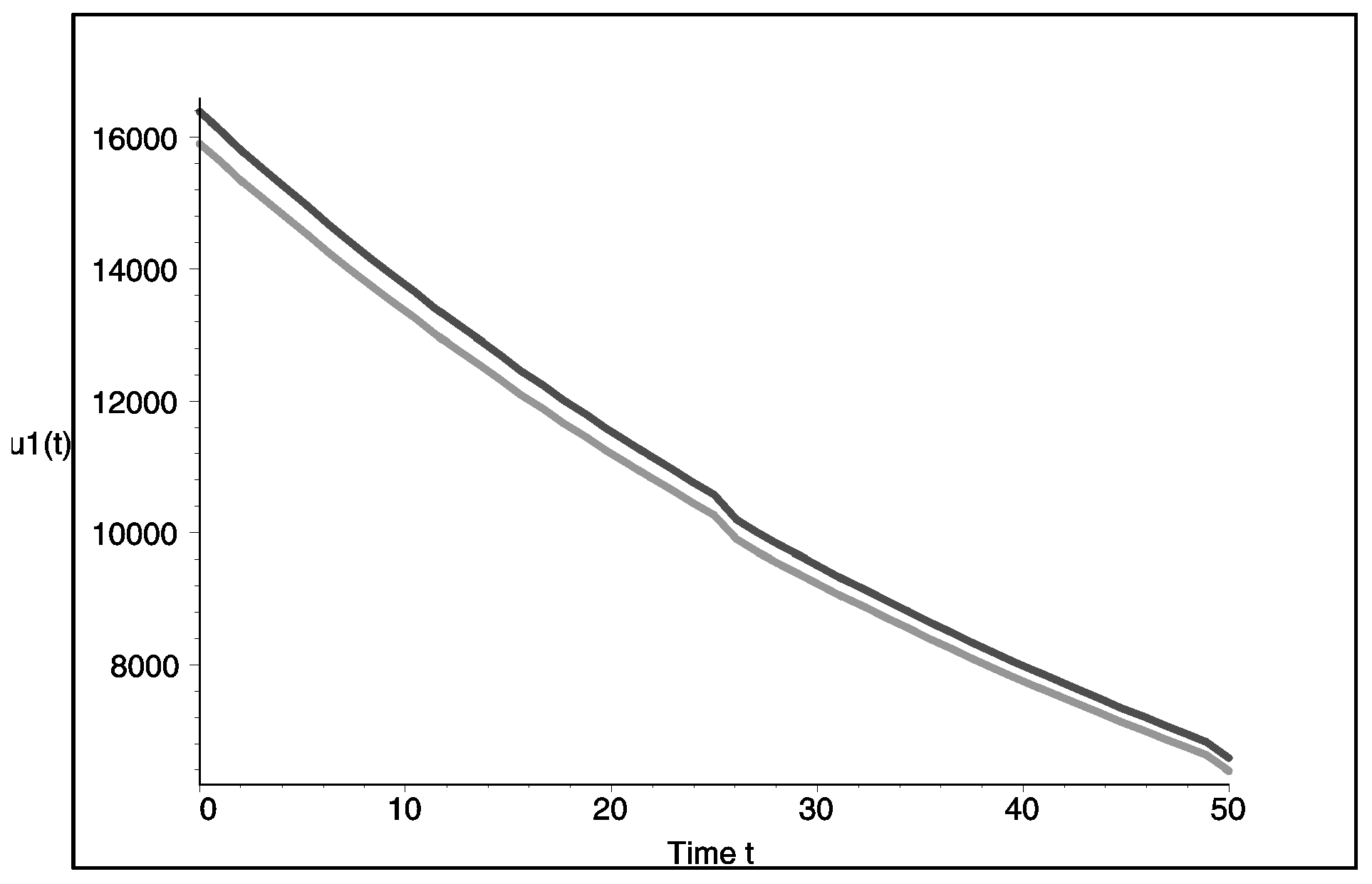
We performed a numerical simulation for a 50-step game with the following parameters:
5. Conclusions
An approach to constructing cooperative equilibrium in multicriteria dynamic games with finite horizon is presented. Cooperative behavior design was performed adopting the Nash bargaining solution. First, we evaluated the multicriteria Nash equilibrium strategies, and players’ payoffs played the role of the status quo points [3]. Then, we constructed the multicriteria cooperative strategies and payoffs via the bargaining scheme.
We studied a bicriteria discrete-time bioresource management problem, where the players differ in their aims and have finite planning horizons. Multicriteria Nash and cooperative equilibria strategies were derived analytically in linear forms, which allows their direct application to concrete populations with appropriate parameters. The results of numerical modeling showed that the presented approach stimulates cooperation, as it more beneficial for players to cooperate. Moreover, an important result related to ecological systems is that the cooperative behavior determined in such way leads to sparing the exploitation rate and improves the ecological situation.
Funding
This research was supported by the Russian Science Foundation, project no. 17-11-01079.
Conflicts of Interest
The author declares no conflict of interest.
References
- Voorneveld, M.; Grahn, S.; Dufwenberg, M. Ideal equilibria in noncooperative multicriteria games. Math. Methods Oper. Res. 2000, 52, 65–77. [Google Scholar] [CrossRef] [Green Version]
- Pusillo, L.; Tijs, S. E-equilibria for multicriteria games. Ann. ISDG 2013, 12, 217–228. [Google Scholar]
- Rettieva, A.N. Equilibria in dynamic multicriteria games. IGTR 2017, 19, 1750002. [Google Scholar] [CrossRef]
- Shapley, L.S. Equilibrium points in games with vector payoffs. Nav. Res. Logist. Q. 1959, 6, 57–61. [Google Scholar] [CrossRef]
- Patrone, F.; Pusillo, L.; Tijs, S.H. Multicriteria games and potentials. TOP 2007, 15, 138–145. [Google Scholar] [CrossRef] [Green Version]
- Pieri, G.; Pusillo, L. Multicriteria Partial Cooperative Games. Appl. Math. 2015, 6, 2125–2131. [Google Scholar] [CrossRef]
- Rettieva, A.N. A discrete-time bioresource management problem with asymmetric players. Autom. Remote Control 2014, 75, 1665–1676. [Google Scholar] [CrossRef]
Figure 1.
Population size: dark—cooperation, light—Nash equilibrium.

Figure 2.
Player 1’s catch: dark—cooperation, light—Nash equilibrium.

© 2018 by the author. Licensee MDPI, Basel, Switzerland. This article is an open access article distributed under the terms and conditions of the Creative Commons Attribution (CC BY) license (http://creativecommons.org/licenses/by/4.0/).
Share and Cite
MDPI and ACS Style
Rettieva, A. Dynamic Multicriteria Games with Finite Horizon. Mathematics 2018, 6, 156. https://doi.org/10.3390/math6090156
AMA Style
Rettieva A. Dynamic Multicriteria Games with Finite Horizon. Mathematics. 2018; 6(9):156. https://doi.org/10.3390/math6090156
Chicago/Turabian StyleRettieva, Anna. 2018. "Dynamic Multicriteria Games with Finite Horizon" Mathematics 6, no. 9: 156. https://doi.org/10.3390/math6090156
Note that from the first issue of 2016, this journal uses article numbers instead of page numbers. See further details here.