A Multi-Objective DV-Hop Localization Algorithm Based on NSGA-II in Internet of Things

1
Complex System and Computational Intelligent Laboratory, Taiyuan University of Science and Technology, Taiyuan 030024, China
2
School of Information, Beijing Wuzi University, Beijing 101149, China
3
Department of Computer Science and Software Engineering, Swinburne University of Technology, Melbourne 3000, Australia
*
Authors to whom correspondence should be addressed.
Mathematics 2019, 7(2), 184; https://doi.org/10.3390/math7020184
Submission received: 17 December 2018
/
Revised: 6 February 2019
/
Accepted: 7 February 2019
/
Published: 15 February 2019
(This article belongs to the Special Issue Evolutionary Computation)
Abstract
:Locating node technology, as the most fundamental component of wireless sensor networks (WSNs) and internet of things (IoT), is a pivotal problem. Distance vector-hop technique (DV-Hop) is frequently used for location node estimation in WSN, but it has a poor estimation precision. In this paper, a multi-objective DV-Hop localization algorithm based on NSGA-II is designed, called NSGA-II-DV-Hop. In NSGA-II-DV-Hop, a new multi-objective model is constructed, and an enhanced constraint strategy is adopted based on all beacon nodes to enhance the DV-Hop positioning estimation precision, and test four new complex network topologies. Simulation results demonstrate that the precision performance of NSGA-II-DV-Hop significantly outperforms than other algorithms, such as CS-DV-Hop, OCS-LC-DV-Hop, and MODE-DV-Hop algorithms.
1. Introduction
As the hottest research topics currently, internet of things (IoT) contains many technologies such as cyber physical systems [1,2], embedded system technology, network information technology, and so on. And wireless sensor networks (WSNs) [3,4], as an important branch of cyber physical systems, have become an innovation and area of research under the spotlight worldwide. Moreover, WSNs technology is so popular that it has been applied in various fields, including the military and national defense, industry [5], disaster relief, medical treatment, environmental monitoring [6], and so on [7]. However, for most WSNs applications, sensor node location information plays a key role; generally, the information obtained from WSNs would be meaningless, if sensor node locations were unknown in applications such as smart grid, object tracking, and location-based routing. Hence, the sensor node localization technology is a critical issue in the rapid development of WSNs and even IoT technology.
Currently, the BeiDou navigation satellite system (BDS) [8,9] and global positioning system (GPS) [10] are generally considered to be the most capable systems for obtaining the exact location. However, it’s worth mentioning that due to the expensive cost, it is almost impossible to complete the full coverage installation of BDS equipment in the whole WSNs. Besides, its positioning accuracy is invariably not satisfactory enough in some special contexts, including the indoor, mine tunnel, canyon, and other complex environments. As a result, it has begun to receive researchers’ attention that the use of interactions and connectivity information between sensor nodes for positioning. Using this information, researchers have proposed a series of localization algorithms. These algorithms are generally classified as a range-based localization algorithm or range-free localization algorithm, depending on whether they are independent of the additional hardware devices. These hardware devices are necessary to obtain the requisite information for the range-based localization algorithm, such as point-to-point distances and angles between sensor nodes. The information between the sensor nodes ensures that the range-based algorithm can achieve accurate positioning, including RSSI [11], ToA [12], and AoA [13], but it requires extensive time and a mass of energy. In contrast, the range-free localization algorithm only needs to ensure the connectivity between sensor nodes, including APIT [14], Centroid [15], Amorphous [16], and DV-Hop [17]. Due to cost constraints, it’s widely used in a large and complex network.
DV-Hop localization algorithm, as a representative range-free positioning algorithm, has garnered extensive attention because of its simple positioning principle. Its main principle is that the beacon nodes (node location information is known) use the connectivity between nodes to send packets to other nodes in the network to obtain the minimum hop count between the beacon nodes and unknown nodes (node location information is unknown). And then, the average distances per hop of beacon nodes are calculated using the position and hop count information of the beacon nodes. Finally, the locations of the unknown nodes are estimated by calculating the distance between the unknown nodes to each beacon node. Compared to other range-free positioning algorithms, it is easier to bring into operation, but the low positioning accuracy has become a problem to be solved. For this reason, scholars propose various improved algorithms based on DV-Hop localization algorithm, including the deterministic algorithms [18,19,20] and bio-inspired optimization algorithms. In addition, Mobility-Assisted Localization in WSNs has also been widely studied by scholars, such as Rezazadeh [21], who proposed a path planning mechanism to improve the accuracy of mobile assisted localization. Alomari improved the path planning method and proposed a path planning strategy based on dynamic fuzzy-logic [22], and proposed an obstacle avoidance strategy based on swarm intelligence optimization [23].
In recent years, with the excellent performance of intelligent computing in various complex optimization problems, various bionic algorithms have been proposed, such as particle swarm optimization (PSO) [24], ant colony optimization (ACO) [25], bat algorithm (BA) [26,27,28], Differential Evolution (DE) [29], Firefly algorithm (FA) [30,31,32], and so on [33]. Compared with the mathematics optimization methods, these biological inspired algorithms show some unique advantages. First, they don’t depend on the requirement of any gradient information in the variable space; in addition, they are insensitive to the initial value and insusceptible to local entrapment. These optimization algorithms play a very good role in practical applications, such as [34,35,36,37,38,39,40], however, with the increasing amount of data in the IoT era, many problems in the real world include multiple decision variables and evaluation indicators. Single-objective optimization has gradually revealed defects for solving such problems. For this reason, multi-objective optimization algorithms based on bionics have also been proposed and are used in various fields, including Multi-Objective Particle Swarm Optimizers (MOPSO) [41,42], multi-objective evolutionary algorithm based on decomposition (MOEA/D) [43], hybrid multi-objective cuckoo search (HMOCS) [44,45], and so on [46,47].
In this paper, we propose a multi-objective DV-Hop localization algorithm based on NSGA-II [48] to solve the sensor node localization problem in WSNs. The remainder of this paper is arrayed as follows. In Section 2, DV-Hop with optimization algorithms and problems are reviewed. In Section 3, standard DV-Hop and NSGA-II are presented. In Section 4, a multi-objective DV-Hop localization model is structured and NSGA-II-DV-Hop is proposed. Simulation results and performance analysis are summarized in Section 5. Lastly, the conclusion is summarized in Section 6.
2. Related Works
In the last few years, with the maturity of various stochastic optimization algorithms in theory, more attention has been paid to the practical application of the algorithm. In 1975, Holland [49] proposed the theory and method of genetic algorithm by studying the genetic evolution process in the natural environment. And after a series of research work, Goldberg [50] formally presented the genetic algorithm (GA) in 1989. In 2007, on the basis of solving the numerical optimization by genetic algorithm, Nan [51] proposed to apply the real-coded GA to WSNs. And in 2010, Gao [52] developed an improved GA to solve wireless sensor localization problem in WSNs. Moreover, Bo [53] also applied GA to solve the problem of WSNs location, and proposed a population constraint strategy based on three beacon nodes to solve the feasible domain of the population.
Furthermore, Yang [54] presented a cuckoo search (CS) algorithm based on Levy flights in 2009. In 2014, Sun [55] developed the CS algorithm and applied it to the DV-Hop positioning algorithm and achieved good positioning results. Based on this, Zhang [56] proposed a weight-oriented CS algorithm (WOCS), and combined it with DV-Hop to locate the unknown sensor nodes in WSNs. The paper improved the search ability of the CS algorithm for unknown nodes by limiting the hop count (which is the minimum hop count between the unknown nodes and each beacon node) in the DV-Hop algorithm. Furthermore, Cui [57] further developed the WOCS algorithm, and proposed an oriented CS algorithm based on the Lévy-Cauchy distribution (OCS-LC) in 2017. This improved strategy is applied to solve the positioning problem of sensor nodes in WSN, and compared with the CS algorithm, there is a large performance improvement when the number of sensor nodes is small. However, these studies were based on the study of the location performance of sensor nodes in a large area, but ignored the positioning performance of sensor nodes in complex terrain. In response to this phenomenon, Cui [58] studied the positioning performance of sensor nodes in C-shaped random and C-shaped grids in 2018. Nevertheless, in this research, the nodes in the network are required to obey Uniform distribution, which is unimaginable in practical production applications. Not only is this so, a common feature of these studies is that more effort is devoted to the improvement of algorithmic search strategies, while ignoring improvements to the original model.
In these studies, although the positioning accuracy has been improved, there are some defects. According to the calculation formula (Equation (7)) of the single-objective model, the population gradually converges to the estimated position as the number of iterations increases, as shown in Figure 4 of the part IV. The actual position of the unknown node is , but the population will converge to the and points, which will bring a large error.
To solve this problem, we propose three other complex terrains for research, including coal mine tunnels [59,60], lake terrain, and canyons terrain. In these specific cases, for the distribution of sensor nodes some new features emerge. For instance, in the coal mine tunnel, the nodes are distributed in narrow tunnels that are interlaced, and the nodes are densely distributed. This requires the algorithm to have a good positioning effect when the number of nodes and the number of beacon nodes are large. However, in the lake terrain, the nodes are distributed around the lake, which leads to communication difficulty when the communication radius is small. Therefore, the algorithm is required to have a strong positioning capability when the communication radius is small and the number of nodes is small. And in the canyons terrain, the nodes are distributed in the canyon among several mountains. In this case, the algorithm is required to have better stable positioning accuracy when the radius and the beacon nodes are small. So, in this paper, we propose a multi-objective DV-Hop localization algorithm based on NSGA-II. The biggest highlight of this paper is to abandon the idea that scholars blindly improve the algorithm search strategy, and change the objective function model in the algorithm to achieve more precise positioning of unknown nodes. A constraint strategy based on all beacon nodes is proposed based on the three beacon nodes constraint strategy.
3. DV-Hop Algorithm and NSGA-II Algorithm
3.1. DV-Hop Algorithm
In this subsection, we will detail the specific implementation process of the DV-Hop algorithm.
Phase 1: Communication detection and broadcasting phase.
At this stage, it is mainly to detect whether direct communication between any two nodes is possible, and also to record the minimum hops count that nodes can communicate with each other. The specific process is that each beacon node broadcasts a packet to the network (the packet includes its location and its own minimum hop count information to other nodes), and the initialization value of each node hop count information is 0. Each time the packet is forwarded, the number of hop count is increased by one. Among them, each node only records the minimum hop count information between it and other nodes.
Phase 2: Distance estimation phase.
Since the position information of the beacon node is known, the (the average distance per hop between any two beacon nodes) can be obtained by Equation (1).
where , are the coordinates of beacon nodes and respectively, and is the minimum hop count between the beacon nodes which is calculated by Phase 1.
And then, the (the distance between beacon node and unknown node ) is estimated by Equation (2).
where is the minimum hop count between the beacon node and unknown node .
Phase 3: Unknown node coordinate estimation phase.
For the unknown node , if more than three distances have been estimated by Equation (2), the position of the unknown node can be calculated mathematically, such as the trilateral measuring method. The computational equation is
where represents the unknown nodes’ coordinates, denotes the coordinates of beacon node , and denotes the distance estimated by Equation (2).
Convert Equation (3) to a matrix form , where , , and are described as the following Equations (4) and (5), respectively.
Based on Equations (4) and (5), the location of the unknown node can be obtained by the least square method. The calculation equation can be expressed as Equation (6).
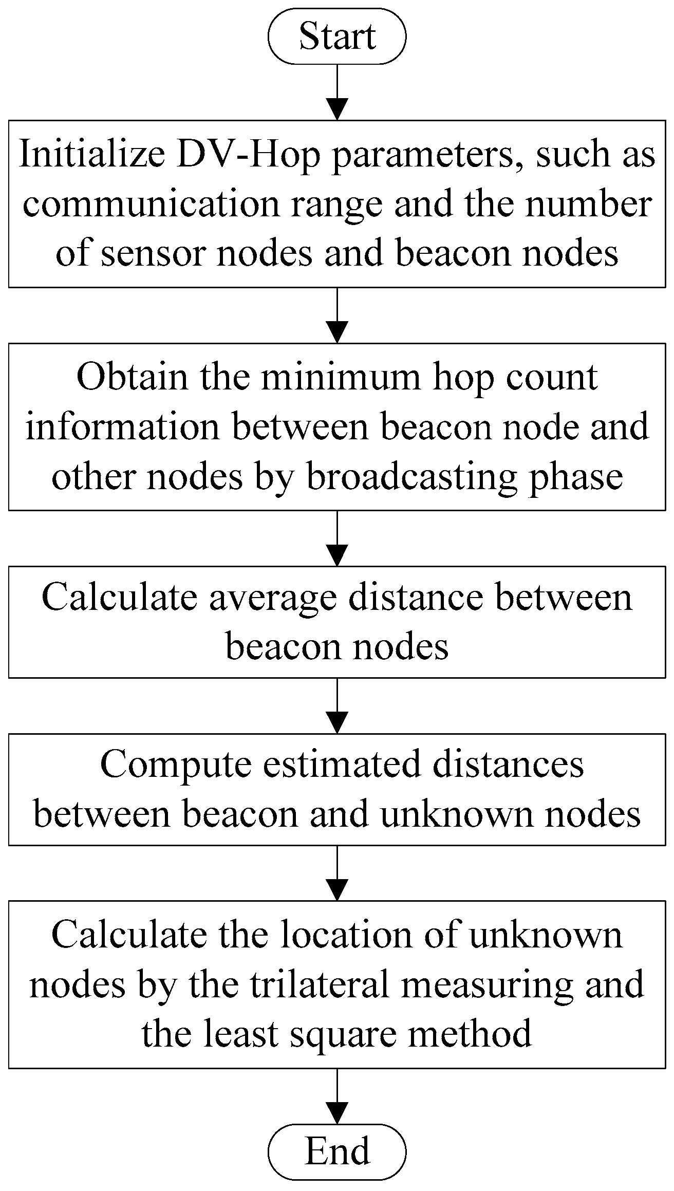
The flowchart of DV-Hop algorithm is introduced in Figure 1.
3.2. NSGA-II Algorithm
A non-dominated sorting genetic algorithm II (NSGA-II) was first proposed in [48] as a biological heuristics algorithm which usually used to solve complex industrial optimization problems. The algorithm has been widely concerned by scholars since its invention due to its faster convergence speed, stronger robustness, and better draw near the true Pareto-optimal front. In NSGA-II algorithm, its core operation contains two parts. One part includes the three traditional operation processes in GA, such as crossover, selection, and mutation; the other part refers to the unique non-dominated sorting operation in the multi-objective optimization algorithm. Therein, the selection operation will retain some of the better individuals with their fitness values (which refer to the non-dominated sorted value). The mutation operation is designed according to the genetic mutation in the biology, in order to ensure that the algorithm has strong global convergence ability. Conversely, the crossover operation is designed based on the principle that homologous chromosomes cross to generate new species to improve the algorithm search ability.
The pseudo-code of NSGA-II algorithm is introduced in Algorithm 1.
| Algorithm 1: The pseudo-code of NSGA-II |
| Begin Input: Population: NP; Dimension: D; Maximum Generation: Gmax; Cross probability: Pc; mutation probability: Pm. Initialization: compute objective values, fast non-dominated sort, selection, crossover and mutation. Generation = 1; While Generation < Gmax do Combine parent and offspring population, compute objective values and fast non-dominated sort. Selection operation. If rand() < Pc Crossover operation; End If rand() < Pm Mutation operation; End Generation = Generation + 1; End Output: The best individuals End |
4. The Proposed Multi-Objective Algorithm
In this paper, we propose a multi-objective DV-Hop localization algorithm based on NSGA-II, which achieves the purpose of improving the positioning accuracy by adopting multi-objective improvement on the original objective.
4.1. The Multi-Objective Model
In the traditional DV-Hop algorithm based on optimization algorithm, Equation (7) is recognized as the most typical objective function.
where denotes the estimated distance in the simulation experiment between beacon node and an unknown node, represents the location of the beacon node , denotes the location of the unknown node, denotes the objective (which refers to one of the objective functions in this paper).
However, this objective function is determined by Equation (8), and Equation (8) is the core theory of the combination of the optimization algorithm and the DV-Hop algorithm. For unknown node , assume is the actual location, and the estimated distances are in the simulation experiment for all beacon nodes, the corresponding errors are . Then, the relationship among them can be expressed as follows: under the premise that the value of is constant, the smaller , the more accurate the positioning accuracy. Therefore, convert Equation (8) to a function form , the objective function is expressed as Equation (7).
Nevertheless, is the unknown node estimated position rather than the actual position, and are obtained in the second phase of the DV-Hop algorithm, and are constant. This means that the position obtained by Equation (7) (the objective function) is closer to the position under the estimated distance, rather than the true exact position. Based on this phenomenon, we present to add an objective function to strengthen the search constraint on the exact position.
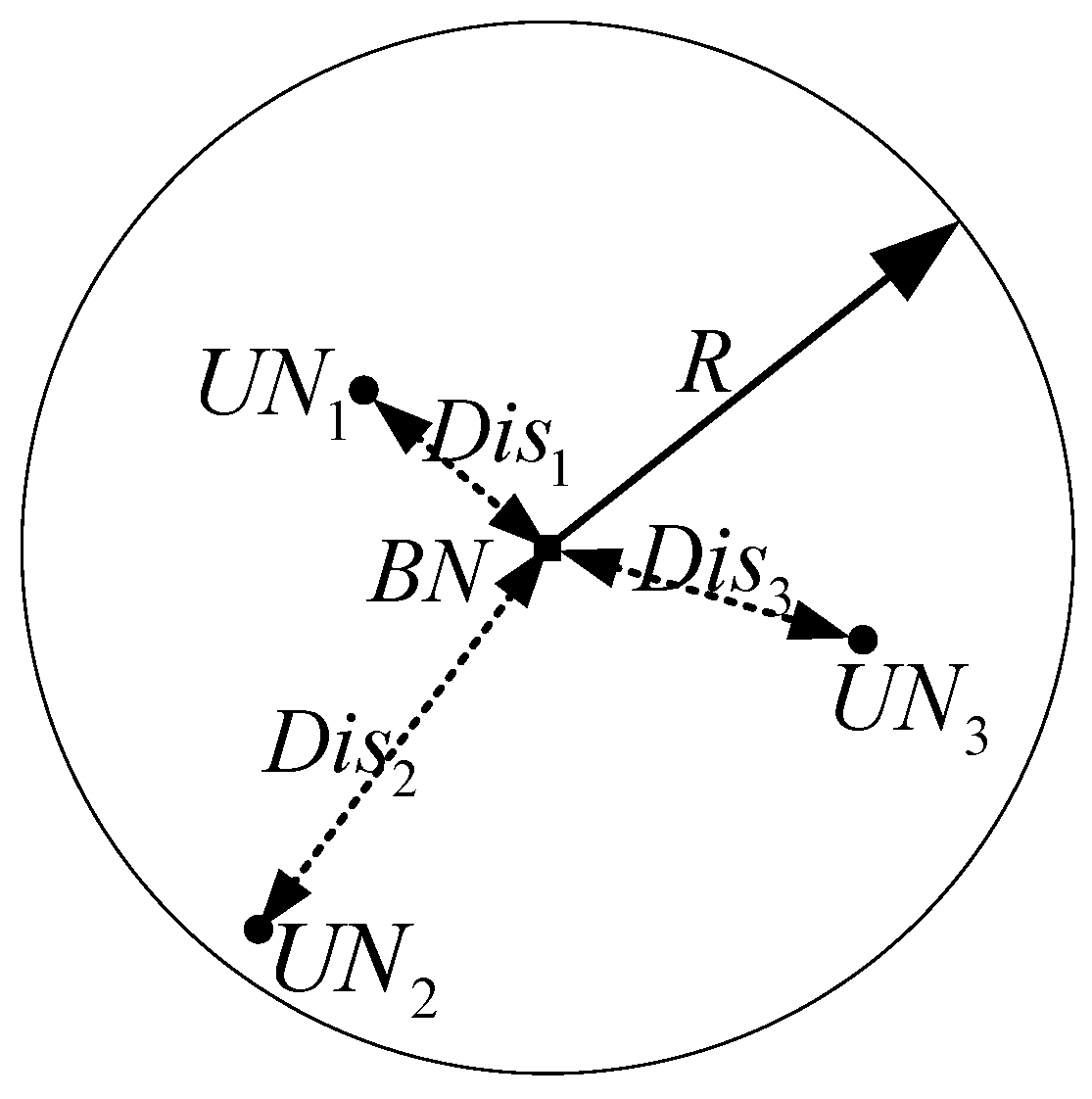
Suppose there are some sensor nodes in the detected area, which contain the beacon nodes and unknown nodes, such as Figure 2. In Figure 2, denotes the beacon node; denote the unknown nodes, respectively; denotes the communication radius; and is the actual distance between and ; the circular area is the communication area of the . When the number of unknown nodes is enough to fill the entire the circular area, the average distance between and is calculated as Equation (9).
denotes the average distance between and , and also represents the average distance per hop between sensor nodes. Particularly, different from is that the calculation result of is the theoretical value of the average distance from the unknown node to the beacon node in per hop. Therefore, the theoretical distance from the unknown node to each beacon node is calculated as Equation (10).
where is the minimum hop count between the beacon node and unknown node .
Similarly, we define the second objective function as follows:
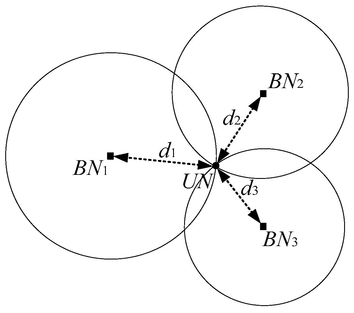
For the sake of clarity, we will elaborate on the difference between our proposed multi-objective and traditional single-objective (We use three beacon nodes and one unknown node for analysis). Figure 3 shows the constraint principle of the objective function in ideal conditions. At the moment, the unknown node in the population finally converges the location of the , and this location is the exact position.
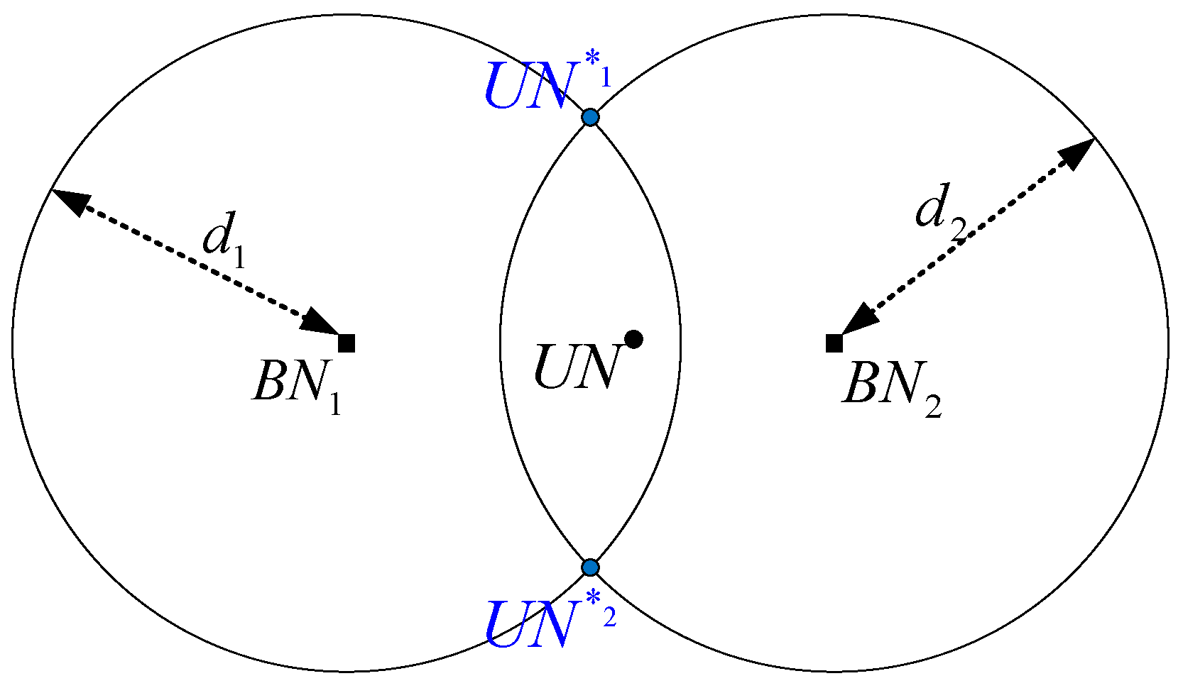
However, the estimated distance is usually accompanied by errors. Therefore, the single-objective function constraint principle in the estimated distance is shown in Figure 4. Where, is defined as the actual location of the unknown node, indicate the beacon nodes, are calculated by Equation (2), represent the estimated location of the unknown node which calculated with Equation (7) in ideal circumstances. It is not difficult to see that the error between the potential optimal solution set found by the single-objective function model and the real position is still large.
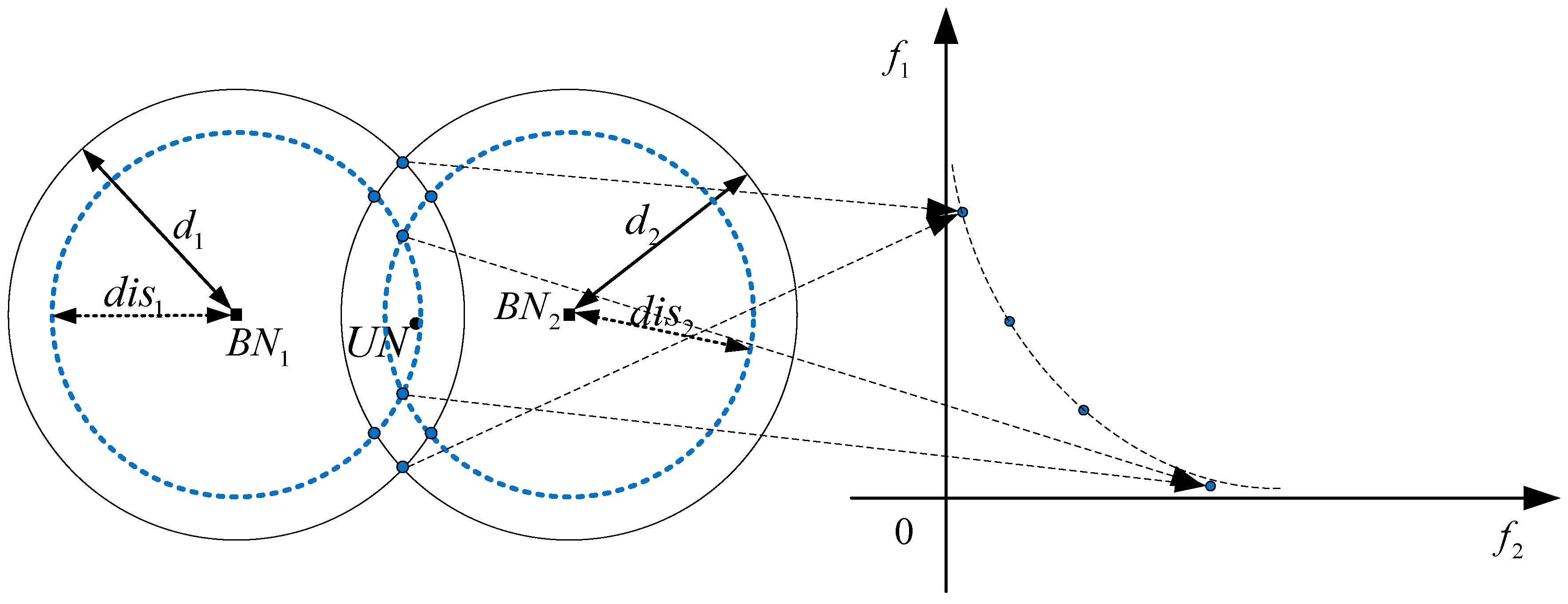
For the defects of single-objective optimization, we propose to use the multi-objective optimization method to reduce the error, such as Figure 5. Figure 5 is composed of two parts, one part is the decision space on the left side and the other part is the objective space on the right side. Where, respectively represent two contradictory objective function models that we proposed, are calculated by Equation (10). As can be seen from the Figure 5, a solution in the objective space corresponds to multiple potential optimal solutions in the decision space. That means that multi-objective models can find more potential optimal solutions in the decision space than the single objective model. Meanwhile, it contains the potential optimal solution that the single-objective model can find. According to this theory, the error of the estimated position obtained by using the multi-objective model must be less than or equal to the single-objective model.
4.2. Population Constraint Strategy
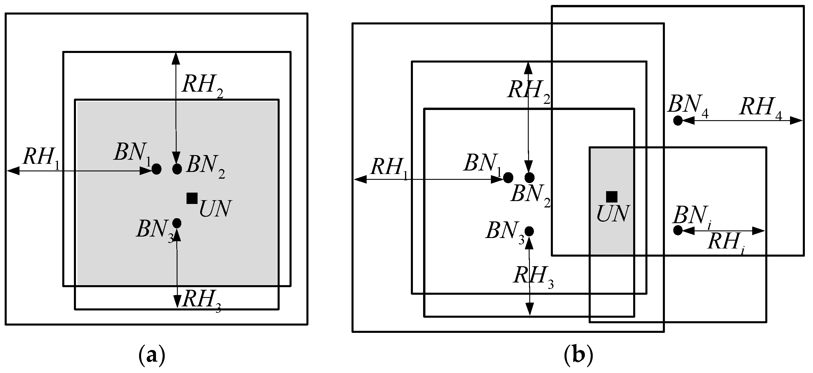
In addition to improvements to the model, this paper also improves the algorithm’s search strategy. In reference [34], the author proposed a population constraint strategy based on three beacon nodes to solve the feasible domain of the population, such as Figure 6a (where denote the beacon nodes, is the unknown node, represent the minimum hop count, represents the radius and the shadow area is the feasible domain). The expression is as follows:
However, when the distance among the three beacon nodes is relatively close and they are located on the same side of the unknown node, the feasible domain of the population is still larger. In this situation, the robustness of the positioning accuracy deteriorates. In this paper, we propose a population constraint strategy based on all beacon nodes, such as Figure 6b. The expression is as follows:
As the number of beacon nodes increases, the probability of the beacon nodes being on the same side of the unknown node decreases correspondingly. This means that the constraint enhancement from the beacon nodes has different directions, and thus the population feasible region decreases. As shown in Figure 6b, the feasible domain of population is significantly reduced compared to Figure 6a. By reducing the feasible region of the population, the convergence speed of the algorithm can be accelerated and the positioning accuracy improved.
4.3. NSGA-II-DV-Hop Algorithm
The construction process of the multi-objective model was introduced before. In this section, the solution process of the model will be introduced. NSGA-II is considered by this paper to be a feasible and reliable algorithm for solving multi-objective models. The pseudo-code of NSGA-II-DV-Hop is introduced in Algorithm 2.
| Algorithm 2: The pseudo-code of NSGA-II-DV-Hop |
| Begin Input: Communication radius, number of nodes, beacon nodes, and the location of beacon nodes; Population: NP; Dimension: D; Maximum Generation: Gmax; Cross probability: Pc; mutation probability: Pm. DV-Hop algorithm with Figure 1. Initialization: Compute objective values with Equation (7) and Equation (11), fast non-dominated sort, selection, crossover and mutation. Population constraint strategy with Equation (13). Generation = 1; While Generation < Gmax do Combine parent and offspring population; compute objective values with Equation (7), Equation (11), and fast non-dominated sort. Selection operation. If rand() < Pc Perform cross-operations on the positions of different individuals in the population; End If rand() < Pm Randomly generate a position that satisfies the boundary condition; End If (the position is contradictory with the boundary condition) Randomly generate a position that satisfies the boundary condition. End Generation = Generation + 1; End Calculate average localization error with Equation (14). Output: The best location and average localization error. End |
5. Experimental Results and Analysis
5.1. Experimental Environment and Evaluation Criteria
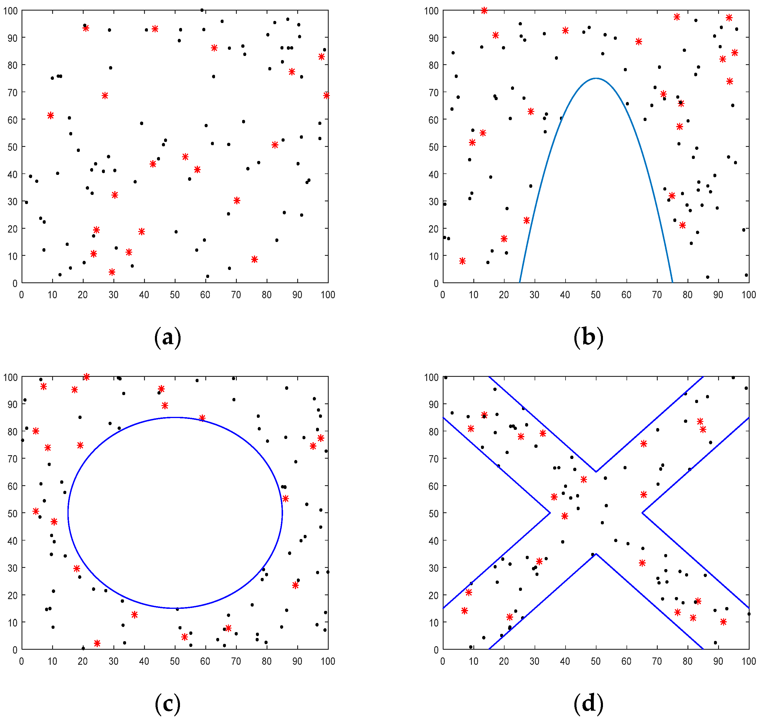
To verify the effectiveness of NSGA-II-DV-Hop, extensive experiments were conducted in MATLAB 2016a. Experimental results will be compared with other three algorithms, including the DV-Hop, CS-DV-Hop, OCS-LC-DV-Hop, and MODE-DV-Hop. Experiment content tests the four different complex networks, including the Random, C-shaped random, O-shaped random, and X-shaped random, as shown in Figure 7. These different network topologies represent different application backgrounds, including plain terrain, canyons terrain, lake terrain, and coal mine tunnels (where all nodes are randomly employed). In addition, the detected area is a square region, and other parameters are listed in Table 1.
In order to compare the positioning performance of different algorithms more fairly, the average localization error (ALE) of unknown nodes is employed as the evaluation criterion. The specific calculation formula is as follows:
where and note the number of unknown nodes and communication radius respectively; represents the estimated location and denotes the exact location.
5.2. Two Objective Function Relationships
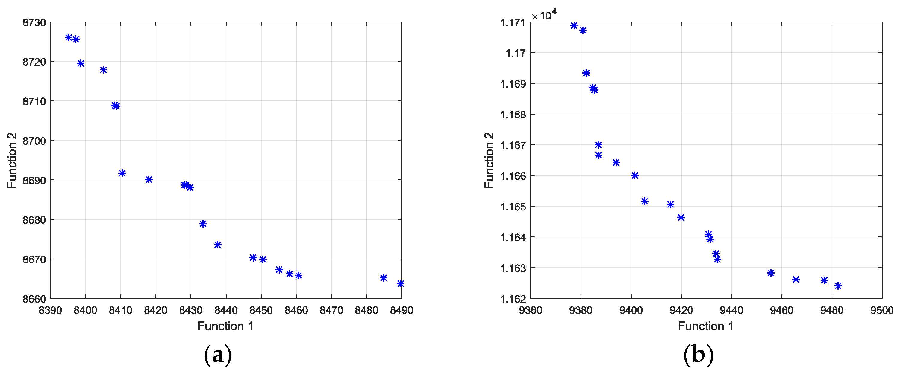
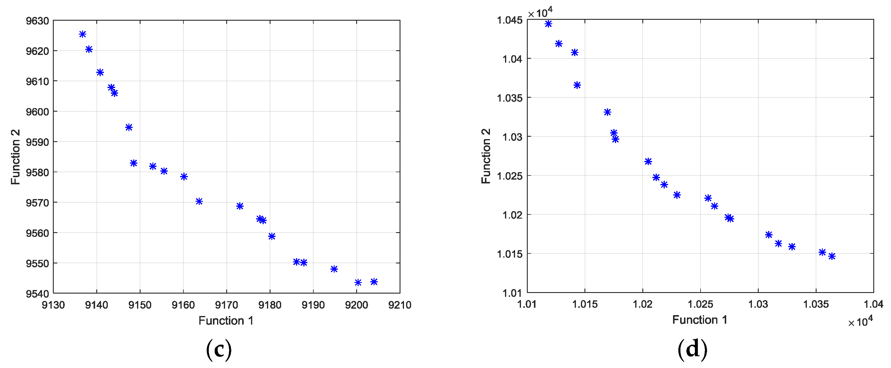
In order to verify whether the multi-objective DV-Hop localization algorithm based on NSGA-II proposed in this paper is feasible, we performed the relationship between two objective functions in different network topologies. The results are shown in Figure 8. In Figure 8a–d respectively show the relationship between the two objective functions in four network topologies, and these relationships are contradictory. The experimental results also demonstrate that the method we proposed is feasible.
In addition, in multi-objective optimization, the solutions obtained after the optimization completed are the Pareto-optimal solutions. These equivalent solutions can be selected according to the actual situation. In this paper, to make the operation simpler, the minimum value of the sum of the two objective values in the solution set is identified as the optimal solution for comparison.
5.3. Influence of Communication Radius
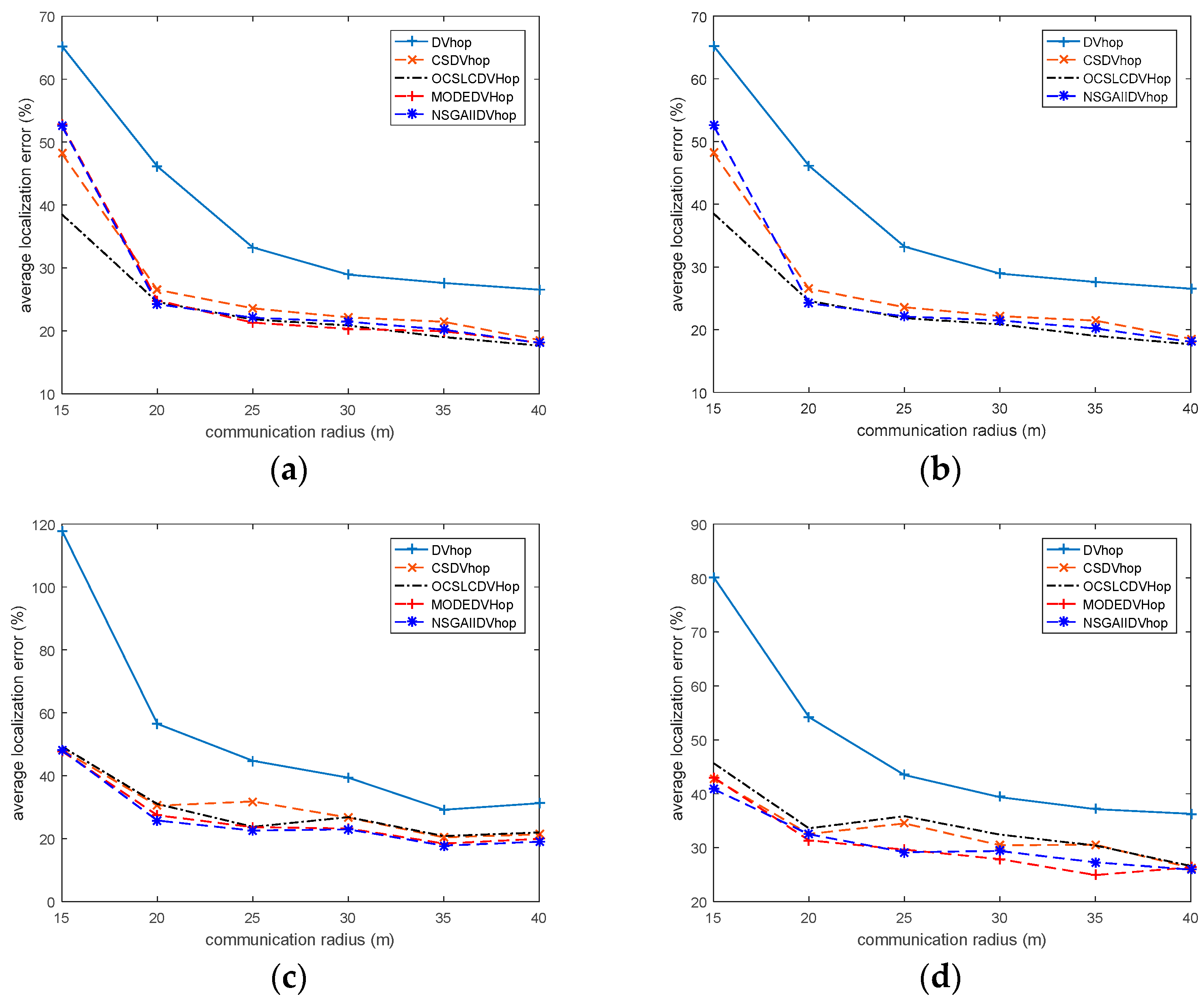
In this experimental phase, the influences of different communication radius on the localization performance are performed. And the communication radius will change from 15 to 40, when the number of nodes and the beacon nodes remain unchanged. The simulation results are shown in Table 2 and Figure 9a–d.
Figure 9a shows the ALE of four algorithms in random topology, and in this topology, NSGA-II-DV-Hop is slightly inferior to the CS-DV-Hop and OCS-LC-DV-Hop algorithm, but significantly better than the DV-Hop algorithm. However, in the other three network topologies (Figure 9b–d, the ALE of NSGA-II-DV-Hop always has the lowest localization error no matter what kind of communication radius.
From Table 2, compared with DV-Hop, NSGA-II-DV-Hop can reduce a maximum of 21.91%, 114.77%, 69.71%, and 39.29% on localization errors, respectively. In particular, in the C-shaped random network topology, compared with CS-DV-Hop and OCS-LC-DV-Hop, the positioning accuracy of the NSGA-II-DV-Hop algorithm is improved by 26.74% and 24.42%, respectively. In addition, the performance of MODE-DV-Hop is similar to NSGA-II-DV-Hop.
5.4. Influence of Nodes
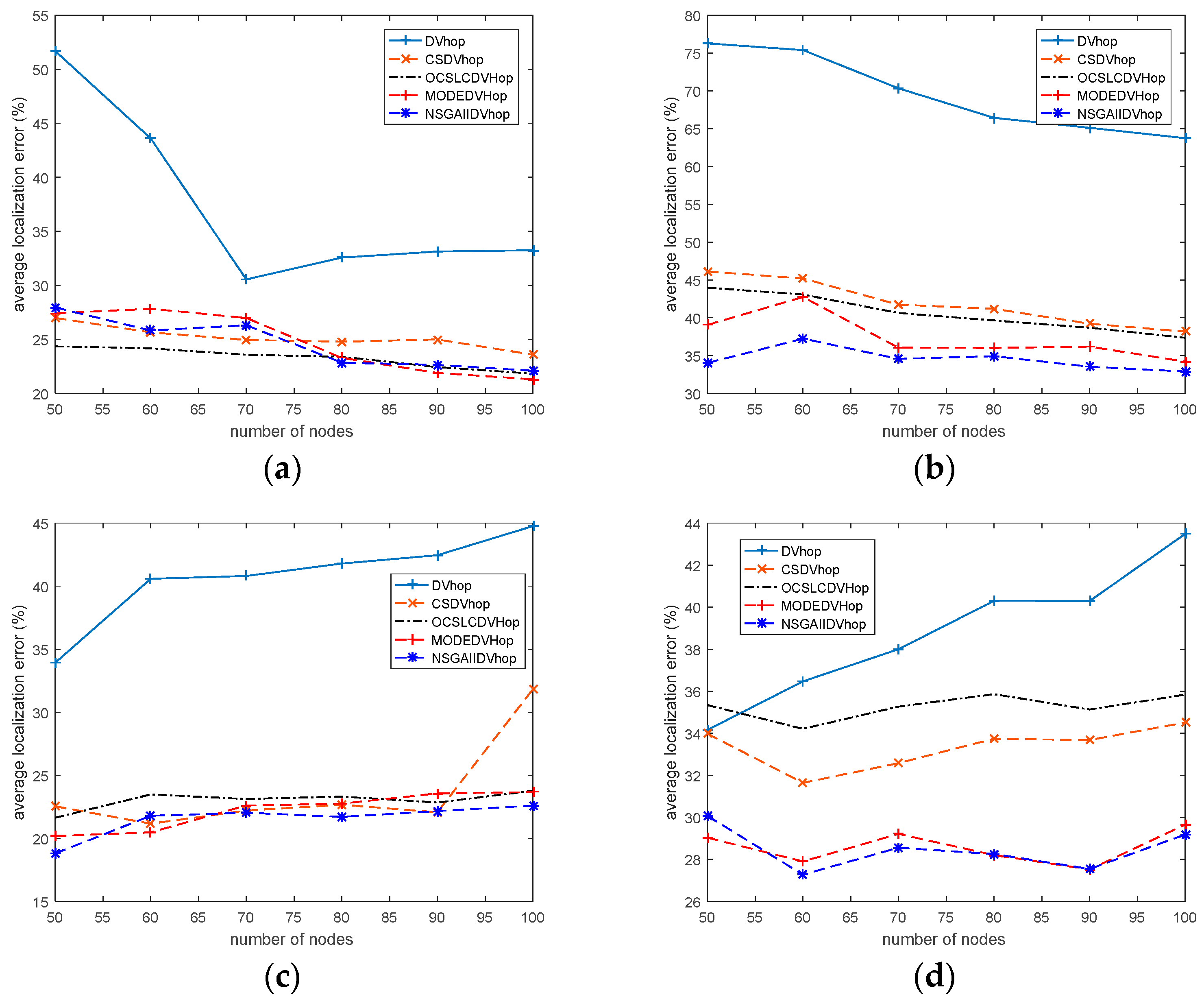
The number of nodes incrementally increases from 50 to 100 in this simulation phase, and the number of beacon nodes and communication radius stay the same. The experiment results are given in Table 3 and Figure 10.
From Figure 10, we can see that in C-shaped and X-shaped random network topologies, the localization accuracy of NSGA-II-DV-Hop and MODE-DV-Hop algorithms are significantly superior to CS-DV-Hop, OCS-LC-DV-Hop, and DV-Hop algorithms. And in the Random or O-shaped network topologies, the performance of NSGA-II-DV-Hop is slightly better than the CS-DV-Hop and OCS-LC-DV-Hop, but always superior to the DV-Hop algorithm.
As depicted in Table 3, NSGA-II-DV-Hop has excellent positioning performance. Compared with the DV-Hop localization algorithm, the ALEs of NSGA-II-DV-Hop are less than 4.25–23.75%, 30.84–42.26%, 15.13–22.18%, and 4.09–14.31% respectively. The most conspicuous improvement occurs in X-shaped and C-Shaped topologies, and the ALEs are reduced by 7.61% and 9.97% more than OCS-LC-DV-Hop algorithm, respectively. Compared with the MODE-DV-Hop, the precision of the NSGA-II-DV-Hop is slightly better.
5.5. Influence of Beacon Nodes
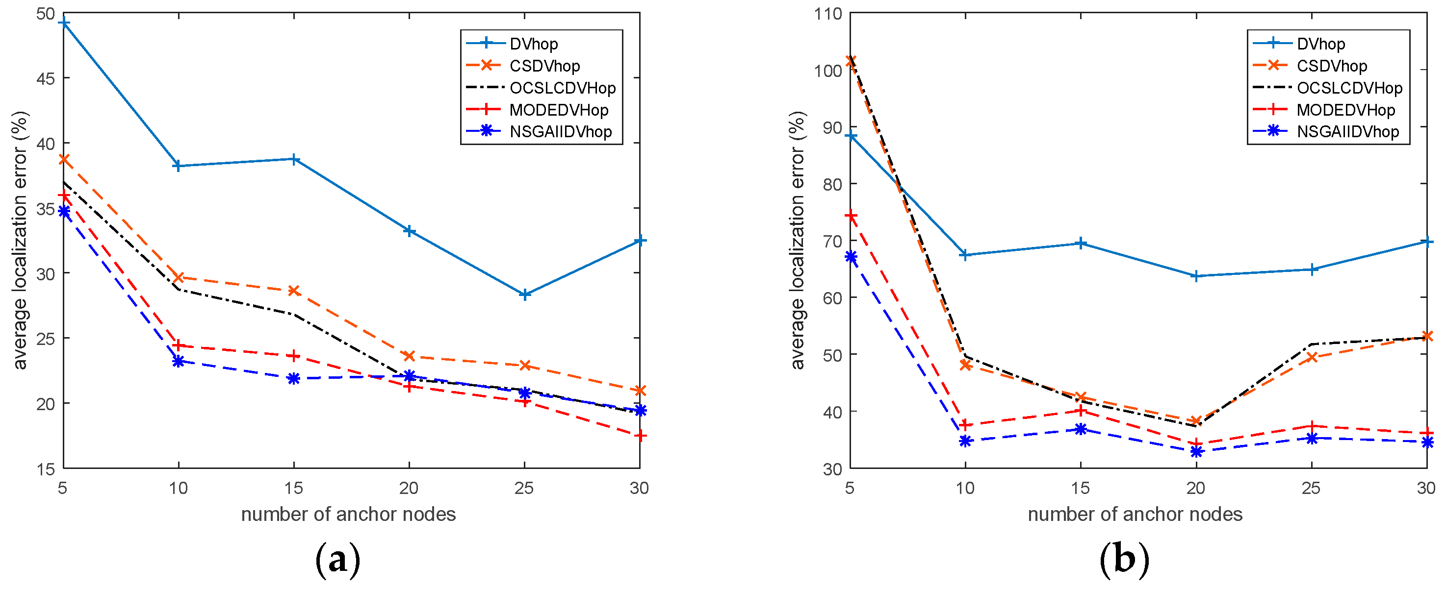
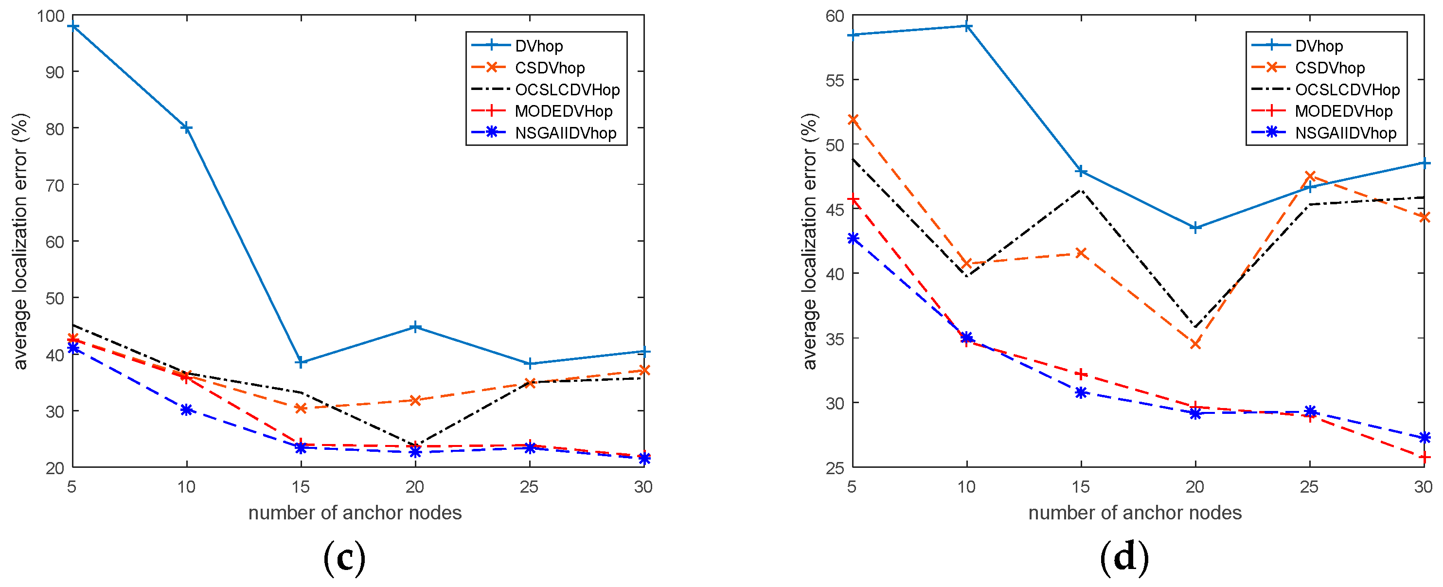
In this simulation phase, the number of beacon nodes incrementally increases from 5 to 20, and the number of nodes and communication radius remain the same. The experiment results are given in Table 4 and Figure 11.
As shown in Figure 11, we can see that the positioning accuracy of NSGA-II-DV-Hop always has an advantage over the other three localization algorithms no matter which topologies. Furthermore, as the number of beacon nodes increases, the ALEs of NSGA-II-DV-Hop present a declining trend, but the ALE of the other three algorithms fluctuate upwards and downwards. The reason causing this kind of phenomenon is that in the complex network topology, the unknown nodes at the edge of the detected area increases, and the feasible domain of the unknown node satisfies the probability increase of Figure 6a, so that the positioning performance deteriorates. Inversely, the NSGA-II-DV-Hop algorithm proposed in this paper adopts the principle of Figure 6b, which reduces the feasible domain of the unknown node, so that the algorithm has more reliable positioning performance.
As shown in Table 4, the original DV-Hop always has the worst localization performance; and NSGA-II-DV-Hop algorithm has the greatest degree of enhancement no matter which network topologies. Especially, compared with the OCS-LC-DV-Hop, NSGA-II-DV-Hop positioning accuracy increased by up to 35.11% and 18.62% respectively in C-shaped and X-shaped network topologies. And the minimum ALEs always are in NSGA-II-DV-Hop and MODE-DV-Hop.
5.6. The Standard Deviation and the Confidence Intervals
As can be seen from Table 5, the standard deviations of the NSGA-II-DV-Hop and MODE-DV-Hop are larger than the CS-DV-Hop and OCS-LC-DV-Hop, which is because the multi-objective model has more potential optimal solutions, such as Figure 5. However, it is worth paying attention that the confidence intervals of NSGA-II-DV-Hop and MODE-DV-Hop are less than the CS-DV-Hop and OCS-LC-DV-Hop in most cases, which means that the performance of the multi-objective model is reliable.
6. Conclusions
This paper proposes a multi-objective DV-Hop localization algorithm based on NSGA-II called NSGA-II-DV-Hop. To further reduce the positioning error, the traditional DV-Hop localization algorithm based on single-objective optimization algorithm is transformed into a multi-objective DV-Hop localization algorithm. We use the multi-objective constraint approach to reduce the convergence domain of unknown nodes and achieve the purpose of improving positioning accuracy. In addition, we also improve the search strategy of the algorithm, changing the population constraint strategy based on three beacon nodes to the population constraint strategy based on all beacon nodes. The simulation results demonstrate that this improved strategy can effectively reduce the sensitivity of the algorithm positioning performance to the number of beacon nodes. Furthermore, this paper also tests four complex network topologies in different backgrounds, and the experimental results show that NSGA-II-DV-Hop significantly outperforms original DV-Hop, CS-DV-Hop, OCS-LC-DV-Hop, and MODE-DV-Hop in all topologies, which also validates the practicability and reliability of this multi-objective model.
And in the future, we will continue to study the error distribution characteristics of the estimated distance in different network topologies and the construction of multi-objective models when there are obstacles in the network.
Author Contributions
Conceptualization, P.W.; Data curation, P.W. and F.X.; Formal analysis, P.W., H.L., Z.C. and J.C.; Funding acquisition, Z.C.; Methodology, P.W.; Project administration, Z.C.; Writing—original draft, P.W., and H.L.; Writing—review & editing, P.W., H.L. and Z.C.
Acknowledgments
This work is supported by the National Natural Science Foundation of China under Grant No.61806138, No.U1636220, No.61663028 and No.61403271, Natural Science Foundation of Shanxi Province under Grant No.201801D121127, Scientific and Technological innovation Team of Shanxi Province under Grant No.201805D131007, PhD Research Startup Foundation of Taiyuan University of Science and Technology under Grant No.20182002.
Conflicts of Interest
The authors declare no conflict of interest.
References
- Khaitan, S.K.; Mccalley, J.D. Design Techniques and Applications of Cyber physical Systems: A Survey. IEEE Syst. J. 2015, 9, 350–365. [Google Scholar] [CrossRef]
- Lee, E.A. Cyber Physical Systems: Design Challenges. In Proceedings of the IEEE International Symposium on Object Oriented Real-Time Distributed Computing, Orlando, FL, USA, 5–7 May 2008; pp. 363–369. [Google Scholar]
- Akyildiz, I.F.; Su, W.; Sankarasubramaniam, Y.; Cayirci, E. A survey on sensor networks. IEEE Commun. Mag. 2002, 40, 102–114. [Google Scholar] [CrossRef]
- Guo, P.; Wang, J.; Li, B.; Lee, S.Y. A variable threshold-value authentication architecture for wireless mesh networks. J. Internet Technol. 2014, 15, 929–936. [Google Scholar]
- Wang, Z.; Wang, X.; Liu, L.; Huang, M.; Zhang, Y. Decentralized feedback control for wireless sensor and actuator networks with multiple controllers. Int. J. Mach. Learn. Cybern. 2017, 8, 1471–1483. [Google Scholar] [CrossRef]
- Chandanapalli, S.B.; Reddy, E.S.; Lakshmi, D.R. DFTDT: Distributed functional tangent decision tree for aqua status prediction in wireless sensor networks. Int. J. Mach. Learn. Cybern. 2017, 9, 1419–1434. [Google Scholar] [CrossRef]
- Suo, H.; Wan, J.; Huang, L.; Zou, C. Issues and Challenges of Wireless Sensor Networks Localization in Emerging Applications. In Proceedings of the International Conference on Computer Science and Electronics Engineering, Hangzhou, China, 23–25 March 2012; IEEE Computer Society: Washington, DC, USA, 2012; pp. 447–451. [Google Scholar]
- Yang, Y.X.; Li, J.L.; Xu, J.Y.; Tang, J.; Guo, H.; He, H. Contribution of the Compass satellite navigation system to global PNT users. Sci. Bull. 2011, 56, 2813. [Google Scholar] [CrossRef]
- Montenbruck, O.; Steigenberger, P.; Hugentobler, U.; Teunissen, P.; Nakamura, S. Initial assessment of the COMPASS/BeiDou-2 regional navigation satellite system. GPS Solut. 2013, 17, 211–222. [Google Scholar] [CrossRef]
- Kaplan, E.D. Understanding GPS: Principles and Application. J. Atmos. Sol.-Terr. Phys. 1996, 59, 598–599. [Google Scholar]
- Girod, L.; Bychkovskiy, V.; Elson, J.; Estrin, D. Locating tiny sensors in time and space: A case study. In Proceedings of the IEEE International Conference on Computer Design: VLSI in Computers and Processors, Freiberg, Germany, 18 September 2002; IEEE Computer Society: Washington, DC, USA, 2002; pp. 214–219. [Google Scholar]
- Harter, A.; Hopper, A.; Steggles, P.; Ward, A.; Webster, P. The anatomy of a context-aware application. Wirel. Netw. 2002, 8, 187–197. [Google Scholar] [CrossRef]
- Niculescu, D.; Nath, B. Ad hoc positioning system (APS) using AOA. In Proceedings of the Joint Conference of the IEEE Computer and Communications, San Francisco, CA, USA, 30 March–3 April 2003; pp. 1734–1743. [Google Scholar]
- He, T.; Huang, C.; Blum, B.M.; Stankovic, J.A.; Abdelzaher, T. Range-free localization schemes in large scale sensor networks. In Proceedings of the IEEE Mobicom, San Diego, CA, USA, 14–19 September 2003; pp. 81–95. [Google Scholar]
- Capkun, S.; Hamdi, M.; Hubaux, J.P. GPS-free positioning in mobile ad-hoc networks. In Proceedings of the Hawaii International Conference on System Sciences, Maui, HI, USA, 6 January 2002; p. 10. [Google Scholar]
- Nagpal, R. Organizing a Global Coordinate System from Local Information on an Amorphous Computer. Available online: https://dspace.mit.edu/handle/1721.1/5926 (accessed on 16 December 2018).
- Niculescu, D.; Nath, B. DV Based Positioning in Ad Hoc Networks. Telecommun. Syst. 2003, 22, 267–280. [Google Scholar] [CrossRef]
- Zhao, J.; Jia, H. A hybrid localization algorithm based on DV-Distance and the twice-weighted centroid for WSN. In Proceedings of the IEEE International Conference on Computer Science and Information Technology, Chengdu, China, 9–11 July 2010; pp. 590–594. [Google Scholar]
- Hou, S.; Zhou, X.; Liu, X. A novel DV-Hop localization algorithm for asymmetry distributed wireless sensor networks. In Proceedings of the IEEE International Conference on Computer Science and Information Technology, Chengdu, China, 9–11 July 2010; pp. 243–248. [Google Scholar]
- Qian, Q.; Shen, X.; Chen, H. An Improved Node Localization Algorithm Based on DV-Hop for Wireless Sensor Networks. Comput. Sci. Inf. Syst. 2011, 8, 953–972. [Google Scholar] [CrossRef]
- Rezazadeh, J.; Moradi, M.; Ismail, A.S.; Dutkiewicz, E. Superior Path Planning Mechanism for Mobile Beacon-Assisted Localization in Wireless Sensor Networks. IEEE Sens. J. 2014, 14, 3052–3064. [Google Scholar] [CrossRef]
- Alomari, A.; Phillips, W.; Aslam, N.; Comeau, F. Dynamic Fuzzy-Logic Based Path Planning for Mobility-Assisted Localization in Wireless Sensor Networks. Sensors 2017, 17, 1904. [Google Scholar] [CrossRef] [PubMed]
- Alomari, A.; Phillips, W.; Aslam, N.; Comeau, F. Swarm Intelligence Optimization Techniques for Obstacle-Avoidance Mobility-Assisted Localization in Wireless Sensor Networks. IEEE Access 2017, 2169–3536. [Google Scholar] [CrossRef]
- Kennedy, J.; Eberhart, R. Particle swarm optimization. In Proceedings of the IEEE International Conference on Neural Networks, Perth, WA, Australia, 27 November–1 December 1995; Volume 4, pp. 1942–1948. [Google Scholar]
- Dorigo, M.; Birattari, M.; Stutzle, T. Ant colony optimization-artificial ants as a computational intelligence technique. IEEE Comput. Intell. Mag. 2006, 1, 28–39. [Google Scholar] [CrossRef]
- Cai, X.; Wang, H.; Cui, Z.; Cai, J.; Xue, Y.; Wang, L. Bat algorithm with triangle-flipping strategy for numerical optimization. Int. J. Mach. Learn. Cybern. 2018, 9, 199–215. [Google Scholar] [CrossRef]
- Cai, X.; Gao, X.; Xue, Y. Improved bat algorithm with optimal forage strategy and random disturbance strategy. Int. J. Bio-Inspired Comput. 2016, 8, 205–214. [Google Scholar] [CrossRef]
- Cui, Z.; Li, F.; Zhang, W. Bat algorithm with principal component analysis. Int. J. Mach. Learn. Cybern. 2018. [Google Scholar] [CrossRef]
- Storn, R.; Price, K. Differential evolution: A simple and efficient heuristic for global optimization over continuous space. J. Glob. Optim. 1997, 11, 341–359. [Google Scholar] [CrossRef]
- Wang, H.; Wang, W.; Zhou, X.; Sun, H.; Jia, Z.; Yu, X.; Cui, Z. Firefly algorithm with neighborhood attraction. Inf. Sci. 2017, 382, 374–387. [Google Scholar] [CrossRef]
- Yu, G.; Feng, Y. Improving firefly algorithm using hybrid strategies. Int. J. Comput. Sci. Math. 2018, 9, 163–170. [Google Scholar] [CrossRef]
- Yu, W.X.; Wang, J. A new method to solve optimization problems via fixed point of firefly algorithm. Int. J. Bio-Inspired Comput. 2018, 11, 249–256. [Google Scholar] [CrossRef]
- Deb, S.; Deb, S.; Gao, X.Z.; et al. A new metaheuristic optimization algorithm motivated by elephant herding behaviour. Int. J. Bio-Inspired Comput. 2017, 8, 394–409. [Google Scholar]
- Cui, Z.; Cao, Y.; Cai, X.; Cai, J.; Chen, J. Optimal LEACH protocol with modified bat algorithm for big data sensing systems in Internet of Things. J. Parallel Distrib. Comput. 2017. [Google Scholar] [CrossRef]
- Gao, M.L.; He, X.H.; Luo, D.S.; Jiang, J.; Teng, Q.Z. Object tracking with improved firefly algorithm. Int. J. Comput. Sci. Math. 2018, 9, 219–231. [Google Scholar]
- Arloff, W.; Schmitt, K.R.B.; Venstrom, L. A parameter estimation method for stiff ordinary differential equations using particle swarm optimization. Int. J. Comput. Sci. Math. 2018, 9, 419–432. [Google Scholar] [CrossRef]
- Cortes, P.; Guadix, J.; Muñuzuri, J.; Onoeva, L. A discrete particle swarm optimization algorithm to operate distributed energy generation networks efficiently. Int. J. Bio-Inspired Comput. 2018, 12, 226–235. [Google Scholar] [CrossRef]
- Wang, Y.; Wang, P.; Zhang, J.; Cui, Z.; Cai, X.; Zhang, W.; Chen, J. A Novel Bat Algorithm with Multiple Strategies Coupling for Numerical Optimization. Mathematics 2019, 7, 135. [Google Scholar] [CrossRef]
- Cui, Z.; Xue, F.; Cai, X.; Cao, Y.; Wang, G.; Chen, J. Detectin of malicious code variants based on deep learning. IEEE Trans. Ind. Inform. 2018, 14, 3187–3196. [Google Scholar] [CrossRef]
- Niu, Y.; Tian, Z.; Zhang, M.; Cai, X.; Li, J. Adaptive two-SVM multi-objective cuckoo search algorithm for software defect prediction. Int. J. Comput. Sci. Math. 2018, 11, 282–291. [Google Scholar] [CrossRef]
- Reyes-Sierra, M.; Coello Coello, C.A. Multi-Objective Particle Swarm Optimizers: A Survey of the State-of-the-Art. Int. J. Comput. Intell. Res. 2006, 2, 287–308. [Google Scholar]
- Bougherara, M.; Nedjah, N.; de Macedo Mourelle, L.; Rahmoun, R.; Sadok, A.; Bennouar, D. IP assignment for efficient NoC-based system design using multi-objective particle swarm optimization. Int. J. Bio-Inspired Comput. 2018, 12, 203–213. [Google Scholar] [CrossRef]
- Zhang, Q.; Li, H. MOEA/D: A multi-objective evolutionary algorithm based on decomposition. IEEE Trans. Evol. Comput. 2007, 11, 712–731. [Google Scholar] [CrossRef]
- Zhang, M.; Wang, H.; Cui, Z.; Chen, J. Hybrid multi-objective cuckoo search with dynamical local search. Memet. Comput. 2018, 10, 199–208. [Google Scholar] [CrossRef]
- Cao, Y.; Ding, Z.; Xue, F.; Rong, X. An improved twin support vector machine based on multi-objective cuckoo search for software defect prediction. Int. J. Bio-Inspired Comput. 2018, 11, 282–291. [Google Scholar] [CrossRef]
- Cui, Z.; Zhang, J.; Wang, Y.; Cao, Y.; Cai, X.; Zhang, W.; Chen, J. A pigeon-inspired optimization algorithm for many-objective optimization problems. Sci. China Inf. Sci. 2019. [Google Scholar] [CrossRef]
- Wang, G.; Cai, X.; Cui, Z.; Min, G.; Chen, J. High Performance Computing for Cyber Physical Social Systems by Using Evolutionary Multi-Objective Optimization Algorithm. IEEE Trans. Emerg. Top. Comput. 2017. [Google Scholar] [CrossRef]
- Deb, K.; Pratap, A.; Agarwal, S.; Meyarivan, T.A.M.T. A fast and elitist multi-objective genetic algorithm: NSGA-II. IEEE Trans. Evol. Comput. 2002, 6, 182–197. [Google Scholar] [CrossRef]
- Holland, J.H. Adaptation in Natural and Artificial Systems; The University of Michigan Press: Ann Arbor, MI, USA, 1975. [Google Scholar]
- Goldberg, D.E. Genetic Algorithms in Search, Optimization and Machine Learning; Addison-Wesley Publishing Company: Boston, MA, USA, 1989; pp. 2104–2116. [Google Scholar]
- Nan, G.F.; Li, M.Q.; Li, J. Estimation of Node Localization with a Real-Coded Genetic Algorithm in WSNs. In Proceedings of the 2007 International Conference on Machine Learning and Cybernetics, Hong Kong, China, 19–22 August 2007; pp. 873–878. [Google Scholar]
- Yang, G.; Yi, Z.; Tianquan, N.; Keke, Y.; Tongtong, X. An improved genetic algorithm for wireless sensor networks localization. In Proceedings of the IEEE Fifth International Conference on Bio-Inspired Computing: Theories and Applications, Changsha, China, 23–26 September 2010; pp. 439–443. [Google Scholar]
- Bo, P.; Lei, L. An improved localization algorithm based on genetic algorithm in wireless sensor networks. Cogn. Neurodyn. 2015, 9, 249–256. [Google Scholar]
- Yang, X.S.; Deb, S. Cuckoo search via Levy flights. In Proceedings of the World Congress on Nature & Biologically Inspired Computing, Coimbatore, India, 9–11 December 2009; pp. 210–214. [Google Scholar]
- Sun, B.; Cui, Z.; Dai, C.; Chen, W. DV-Hop Localization Algorithm with Cuckoo Search. Sens. Lett. 2014, 12, 444–447. [Google Scholar] [CrossRef]
- Zhang, M.; Zhu, Z.; Cui, Z. DV-hop localization algorithm with weight-based oriented cuckoo search algorithm. In Proceedings of the Chinese Control Conference, Dalian, China, 26–28 July 2017; pp. 2534–2539. [Google Scholar]
- Cui, Z.; Sun, B.; Wang, G.; Xue, Y.; Chen, J. A novel oriented cuckoo search algorithm to improve DV-Hop performance for cyber-physical systems. J. Parallel Distrib. Comput. 2017, 103, 42–52. [Google Scholar] [CrossRef]
- Cui, L.; Xu, C.; Li, G.; Minga, Z.; Fenga, Y.; Lua, N. A High Accurate Localization Algorithm with DV-Hop and Differential Evolution for Wireless Sensor Network. Appl. Soft Comput. 2018, 68, 39–52. [Google Scholar] [CrossRef]
- Chen, W.; Jiang, X.; Li, X.; Gao, J.; Xu, X.; Ding, S. Wireless Sensor Network nodes correlation method in coal mine tunnel based on Bayesian decision. Meas. J. Int. Meas. Confed. 2013, 46, 2335–2340. [Google Scholar] [CrossRef]
- Farjow, W.; Raahemifar, K.; Fernando, X. Novel wireless channels characterization model for underground mines. Appl. Math. Model. 2015, 39, 5997–6007. [Google Scholar] [CrossRef]
Figure 1.
The distance vector-hop technique (DV-Hop) flowchart.

Figure 2.
Distance relationship of sensor nodes.

Figure 3.
Constraint principle in ideal conditions.

Figure 4.
Single-objective constraint principle.

Figure 5.
Multi-objective constraint principle.

Figure 6.
Population constraint strategy. (a) Population constraint based on three beacon nodes; (b) Population constraint based on all beacon nodes.
Figure 6.
Population constraint strategy. (a) Population constraint based on three beacon nodes; (b) Population constraint based on all beacon nodes.

Figure 7.
Four different complex networks topologies. (a) The random topology; (b) The C-shaped random topology; (c) The O-shaped random topology; (d) The X-shaped random topology.
Figure 7.
Four different complex networks topologies. (a) The random topology; (b) The C-shaped random topology; (c) The O-shaped random topology; (d) The X-shaped random topology.

Figure 8.
Two objective function relationships in four different network topologies. (a) The random topology; (b) The C-shaped random topology; (c) The O-shaped random topology; (d) The X-shaped random topology.
Figure 8.
Two objective function relationships in four different network topologies. (a) The random topology; (b) The C-shaped random topology; (c) The O-shaped random topology; (d) The X-shaped random topology.


Figure 9.
The ALE of four network topologies in different communication radius. (a) The random topology; (b) The C-shaped random topology; (c) The O-shaped random topology; (d) The X-shaped random topology.
Figure 9.
The ALE of four network topologies in different communication radius. (a) The random topology; (b) The C-shaped random topology; (c) The O-shaped random topology; (d) The X-shaped random topology.

Figure 10.
The ALE of four network topologies in different number of nodes. (a) The random topology; (b) The C-shaped random topology; (c) The O-shaped random topology; (d) The X-shaped random topology.
Figure 10.
The ALE of four network topologies in different number of nodes. (a) The random topology; (b) The C-shaped random topology; (c) The O-shaped random topology; (d) The X-shaped random topology.

Figure 11.
The ALE of four network topologies in different number of beacon nodes. (a) The random topology; (b) The C-shaped random topology; (c) The O-shaped random topology; (d) The X-shaped random topology.
Figure 11.
The ALE of four network topologies in different number of beacon nodes. (a) The random topology; (b) The C-shaped random topology; (c) The O-shaped random topology; (d) The X-shaped random topology.


Table 1.
Parameter settings.
| Parameter | Value |
|---|---|
| Pc | 1 |
| Pm | 1/c (c refers to the variable dimension) |
| Population | 20 |
| Largest iterations | 500 |
| R(m) | 25 |
| Nodes | 100 |
| Beacon nodes | 20 |
Table 2.
Average localization error (ALE) of different algorithms in different network topologies and communication radius.
Table 2.
Average localization error (ALE) of different algorithms in different network topologies and communication radius.
| Communication Radius | 15 | 20 | 25 | 30 | 35 | 40 | |
|---|---|---|---|---|---|---|---|
| random topology | DV-Hop | 65.24 | 46.14 | 33.25 | 28.92 | 27.59 | 26.54 |
| CS-DV-Hop | 48.17 | 26.52 | 23.58 | 22.15 | 21.44 | 18.54 | |
| OCS-LC-DV-Hop | 38.52 | 24.58 | 21.83 | 20.84 | 19.01 | 17.65 | |
| MODE-DV-Hop | 52.71 | 24.84 | 21.30 | 20.32 | 19.93 | 18.13 | |
| NSGAII-DV-Hop | 52.57 | 24.23 | 22.09 | 21.46 | 20.19 | 18.06 | |
| C-shaped random topology | DV-Hop | 172.33 | 112.53 | 63.73 | 49.78 | 44.81 | 41.62 |
| CS-DV-Hop | 84.30 | 62.38 | 38.17 | 31.25 | 31.42 | 29.93 | |
| OCS-LC-DV-Hop | 81.98 | 58.59 | 37.35 | 30.46 | 32.09 | 29.36 | |
| MODE-DV-Hop | 66.80 | 51.23 | 34.20 | 30.44 | 27.74 | 28.72 | |
| NSGAII-DV-Hop | 57.56 | 49.54 | 32.89 | 28.89 | 28.87 | 28.37 | |
| O-shaped random topology | DV-Hop | 117.88 | 56.50 | 44.77 | 39.39 | 29.24 | 31.28 |
| CS-DV-Hop | 48.27 | 30.51 | 31.83 | 26.72 | 20.44 | 21.38 | |
| OCS-LC-DV-Hop | 49.32 | 31.05 | 23.77 | 26.86 | 20.85 | 21.98 | |
| MODE-DV-Hop | 47.81 | 27.44 | 23.67 | 23.24 | 18.48 | 19.97 | |
| NSGAII-DV-Hop | 48.17 | 25.78 | 22.59 | 22.96 | 17.80 | 19.06 | |
| X-shaped random topology | DV-Hop | 80.18 | 54.22 | 43.49 | 39.39 | 37.15 | 36.29 |
| CS-DV-Hop | 42.84 | 32.54 | 34.51 | 30.46 | 30.55 | 26.28 | |
| OCS-LC-DV-Hop | 45.68 | 33.60 | 35.84 | 32.43 | 30.41 | 26.60 | |
| MODE-DV-Hop | 43.04 | 31.37 | 29.65 | 27.88 | 24.93 | 26.38 | |
| NSGAII-DV-Hop | 40.89 | 32.49 | 29.18 | 29.39 | 27.30 | 25.93 | |
Table 3.
ALE of different algorithms in different network topologies and number of nodes.
| Number of Nodes | 50 | 60 | 70 | 80 | 90 | 100 | |
|---|---|---|---|---|---|---|---|
| random topology | DV-Hop | 51.70 | 43.60 | 30.56 | 32.57 | 33.13 | 33.25 |
| CS-DV-Hop | 26.98 | 25.65 | 24.94 | 24.78 | 24.99 | 23.58 | |
| OCS-LC-DV-Hop | 24.35 | 24.17 | 23.57 | 23.39 | 22.43 | 21.83 | |
| MODE-DV-Hop | 27.41 | 27.83 | 26.98 | 23.29 | 21.89 | 21.30 | |
| NSGAII-DV-Hop | 27.95 | 25.82 | 26.31 | 22.84 | 22.64 | 22.09 | |
| C-shaped random topology | DV-Hop | 76.27 | 75.39 | 70.34 | 66.42 | 65.12 | 63.73 |
| CS-DV-Hop | 46.12 | 45.19 | 41.73 | 41.18 | 39.21 | 38.17 | |
| OCS-LC-DV-Hop | 43.98 | 43.07 | 40.63 | 39.64 | 38.68 | 37.35 | |
| MODE-DV-Hop | 39.05 | 42.74 | 36.04 | 36.01 | 36.18 | 34.20 | |
| NSGAII-DV-Hop | 34.01 | 37.24 | 34.56 | 34.92 | 33.52 | 32.89 | |
| O-shaped random topology | DV-Hop | 33.92 | 40.59 | 40.82 | 41.80 | 42.46 | 44.77 |
| CS-DV-Hop | 22.54 | 21.16 | 22.20 | 22.66 | 22.06 | 31.83 | |
| OCS-LC-DV-Hop | 21.63 | 23.48 | 23.12 | 23.31 | 22.84 | 23.77 | |
| MODE-DV-Hop | 20.18 | 20.47 | 22.60 | 22.75 | 23.56 | 23.67 | |
| NSGAII-DV-Hop | 18.79 | 21.78 | 22.03 | 21.70 | 22.16 | 22.59 | |
| X-shaped random topology | DV-Hop | 34.16 | 36.47 | 38.00 | 40.31 | 40.30 | 43.49 |
| CS-DV-Hop | 33.98 | 31.64 | 32.58 | 33.74 | 33.68 | 34.51 | |
| OCS-LC-DV-Hop | 35.34 | 34.21 | 35.27 | 35.86 | 35.13 | 35.84 | |
| MODE-DV-Hop | 29.03 | 27.90 | 29.21 | 28.20 | 27.52 | 29.65 | |
| NSGAII-DV-Hop | 30.07 | 27.27 | 28.55 | 28.25 | 27.54 | 29.18 | |
Table 4.
ALE of different algorithms in different network topologies and number of beacon nodes.
| Number of Baecon Nodes | 5 | 10 | 15 | 20 | 25 | 30 | |
|---|---|---|---|---|---|---|---|
| random topology | DV-Hop | 49.21 | 38.21 | 38.77 | 33.25 | 28.31 | 32.48 |
| CS-DV-Hop | 38.76 | 29.67 | 28.59 | 23.58 | 22.88 | 20.94 | |
| OCS-LC-DV-Hop | 36.98 | 28.72 | 26.80 | 21.83 | 21.01 | 19.22 | |
| MODE-DV-Hop | 35.99 | 24.41 | 23.62 | 21.30 | 20.11 | 17.49 | |
| NSGAII-DV-Hop | 34.74 | 23.25 | 21.90 | 22.09 | 20.81 | 19.43 | |
| C-shaped random topology | DV-Hop | 88.45 | 67.42 | 69.45 | 63.73 | 64.88 | 69.80 |
| CS-DV-Hop | 101.44 | 48.14 | 42.49 | 38.17 | 49.41 | 53.24 | |
| OCS-LC-DV-Hop | 102.36 | 49.62 | 41.73 | 37.35 | 51.77 | 52.90 | |
| MODE-DV-Hop | 74.48 | 37.55 | 40.08 | 34.20 | 37.43 | 36.11 | |
| NSGAII-DV-Hop | 67.25 | 34.78 | 36.83 | 32.89 | 35.34 | 34.63 | |
| O-shaped random topology | DV-Hop | 98.08 | 79.95 | 38.47 | 44.77 | 38.28 | 40.49 |
| CS-DV-Hop | 42.65 | 36.22 | 30.35 | 31.83 | 34.84 | 37.10 | |
| OCS-LC-DV-Hop | 45.15 | 36.60 | 33.17 | 23.77 | 34.99 | 35.72 | |
| MODE-DV-Hop | 42.59 | 35.76 | 23.97 | 23.67 | 23.86 | 21.88 | |
| NSGAII-DV-Hop | 41.14 | 30.23 | 23.46 | 22.59 | 23.38 | 21.47 | |
| X-shaped random topology | DV-Hop | 58.46 | 59.14 | 47.89 | 43.49 | 46.66 | 48.57 |
| CS-DV-Hop | 51.90 | 40.74 | 41.54 | 34.51 | 47.54 | 44.36 | |
| OCS-LC-DV-Hop | 48.83 | 39.74 | 46.47 | 35.84 | 45.32 | 45.87 | |
| MODE-DV-Hop | 45.76 | 34.70 | 32.19 | 29.65 | 28.96 | 25.75 | |
| NSGAII-DV-Hop | 42.74 | 35.03 | 30.81 | 29.18 | 29.29 | 27.25 | |
Table 5.
The standard deviation and confidence intervals of different algorithms in four network topologies.
Table 5.
The standard deviation and confidence intervals of different algorithms in four network topologies.
| Random Topology | C-Shaped Random Topology | O-Shaped Random Topology | X-Shaped Random Topology | ||
|---|---|---|---|---|---|
| the standard deviation and the confidence intervals (probably at 95%) | CS-DV-Hop | 0.5636 | 0.5241 | 0.1390 | 0.2150 |
| [0.46, 0.67] | [0.41, 0.70] | [0.11, 0.19] | [0.17, 0.29] | ||
| 23.5816 | 38.1680 | 31.8336 | 34.5050 | ||
| [23.12, 24.03] | [37.97, 38.36] | [31.78, 31.89] | [34.42, 34.59] | ||
| OCS-LC-DV-Hop | 0.9243 | 0.4277 | 0.6448 | 0.1736 | |
| [0.67, 1.31] | [0.34, 0.58] | [0.51, 0.87] | [0.13, 0.23] | ||
| 21.8342 | 37.3458 | 23.7727 | 35.8445 | ||
| [21.04, 22.21] | [37.19, 37.51] | [23.53, 24.01] | [35.77, 35.91] | ||
| MODE-DV-Hop | 1.2770 | 0.7446 | 0.6658 | 1.1133 | |
| [1.02, 1.71] | [0.59, 1.00] | [0.53, 0.89] | [0.88, 1.49] | ||
| 21.3018 | 34.2048 | 23.6688 | 29.6472 | ||
| [20.82, 21.77] | [33.92, 34.48] | [23.42, 23.91] | [29.23, 30.06] | ||
| NSGA-II-DV-Hop | 0.7005 | 0.4887 | 0.4911 | 0.8246 | |
| [0.55, 0.94] | [0.38, 0.66] | [0.39, 0.66] | [0.65, 1.11] | ||
| 22.0850 | 32.8934 | 22.5942 | 29.1820 | ||
| [21.82, 22.35] | [32.71, 33.08] | [22.41, 22.77] | [28.87, 29.48] | ||
© 2019 by the authors. Licensee MDPI, Basel, Switzerland. This article is an open access article distributed under the terms and conditions of the Creative Commons Attribution (CC BY) license (http://creativecommons.org/licenses/by/4.0/).
Share and Cite
MDPI and ACS Style
Wang, P.; Xue, F.; Li, H.; Cui, Z.; Xie, L.; Chen, J. A Multi-Objective DV-Hop Localization Algorithm Based on NSGA-II in Internet of Things. Mathematics 2019, 7, 184. https://doi.org/10.3390/math7020184
AMA Style
Wang P, Xue F, Li H, Cui Z, Xie L, Chen J. A Multi-Objective DV-Hop Localization Algorithm Based on NSGA-II in Internet of Things. Mathematics. 2019; 7(2):184. https://doi.org/10.3390/math7020184
Chicago/Turabian StyleWang, Penghong, Fei Xue, Hangjuan Li, Zhihua Cui, Liping Xie, and Jinjun Chen. 2019. "A Multi-Objective DV-Hop Localization Algorithm Based on NSGA-II in Internet of Things" Mathematics 7, no. 2: 184. https://doi.org/10.3390/math7020184
Note that from the first issue of 2016, this journal uses article numbers instead of page numbers. See further details here.