A Unified Model for Plasticity in Ferritic, Martensitic and Dual-Phase Steels

1
Department of Materials Science and Metallurgy, University of Cambridge, 27 Charles Babbage Road, Cambridge CB3 0FS, UK
2
Nippon Steel Corporation, 1-1 Tsukiji, Kisarazu, Chiba 292-0835, Japan
*
Author to whom correspondence should be addressed.
Metals 2020, 10(6), 764; https://doi.org/10.3390/met10060764
Submission received: 23 April 2020
/
Revised: 28 May 2020
/
Accepted: 2 June 2020
/
Published: 8 June 2020
Abstract
:Unified equations for the relationships among dislocation density, carbon content and grain size in ferritic, martensitic and dual-phase steels are presented. Advanced high-strength steels have been developed to meet targets of improved strength and formability in the automotive industry, where combined properties are achieved by tailoring complex microstructures. Specifically, in dual-phase (DP) steels, martensite with high strength and poor ductility reinforces steel, whereas ferrite with high ductility and low strength maintains steel’s formability. To further optimise DP steel’s performance, detailed understanding is required of how carbon content and initial microstructure affect deformation and damage in multi-phase alloys. Therefore, we derive modified versions of the Kocks–Mecking model describing the evolution of the dislocation density. The coefficient controlling dislocation generation is obtained by estimating the strain increments produced by dislocations pinning at other dislocations, solute atoms and grain boundaries; such increments are obtained by comparing the energy required to form dislocation dipoles, Cottrell atmospheres and pile-ups at grain boundaries, respectively, against the energy required for a dislocation to form and glide. Further analysis is made on how thermal activation affects the efficiency of different obstacles to pin dislocations to obtain the dislocation recovery rate. The results are validated against ferritic, martensitic and dual-phase steels showing good accuracy. The outputs are then employed to suggest optimal carbon and grain size combinations in ferrite and martensite to achieve highest uniform elongation in single- and dual-phase steels. The models are also combined with finite-element simulations to understand the effect of microstructure and composition on plastic localisation at the ferrite/martensite interface to design microstructures in dual-phase steels for improved ductility.
1. Introduction
Further improvement of advanced high strength steels (AHSSs) is required to reduce weight in electric vehicles (EVs), which controls their range of operation, the most crucial factor for their practical use. Although high strength steels (HSSs) have contributed to the reduction of the weight of vehicles, their use is limited to parts of simple geometries, because of their poor formability. AHSS improves both strength and formability by employing several different mechanical characteristics of microstructures that play different roles in the material; typically, martensite with high strength and poor ductility reinforces it, and ferrite with high ductility and low strength maintains its formability. Thus, AHSSs have been widely used for car body parts and reduce much more weight of vehicles than HSSs [1]. That is the reason AHSSs are expected to realise further weight reduction required for EVs. However, its complex microstructure makes it easy to promote voids between different kinds of microstructures. Voids promote ductile fracture and prevent AHSSs’ improvement of formability [2].
Significant efforts have been made to investigate the mechanism of void nucleation and prevention. Dual-phase (DP) steels have been studied often because they consist of ferritic and martensitic grains that are typically contained in AHSS, and the interface between them is known as the typical site for void nucleation because of the large difference in their mechanical characteristics [3,4]. For instance, in-situ scanning electron microscopy (SEM) examination of DP steels conducted by Azuma et al. showed that some voids are generated by fracture of martensitic grains [5]. Furthermore, SEM observations by Archie et al. indicate that voids are produced by debond of prior austenite grain boundaries, accompanied with strain concentration which is expected to be caused by the strength and strain incompatibility between martensitic and ferritic grains [6,7].
Finite element method (FEM) simulations have also been used widely to study deformation and void formation in DP steels. In FEM, the tested material is divided into small elements within a representative volume element, where the different mechanical characteristics are applicable to each elements so that the complex microstructure consisting of two phases in DP steel is explicitly considered [8,9,10,11,12,13,14,15,16,17,18]. FEM also allows us to examine stress and strain distribution of each grain, which is helpful to figure out the relationship between void nucleation and localised ferrite–martensite strain incompatibilities. For instance, Matsuno and Kim conducted FEM simulations with the interfacial debond-based void nucleation model suggested by Xu et al. and subsequent authors [19,20,21]. In those simulations, ferrite–martensite interfaces were assumed to bond by the distance-dependant stress such as inter-atomic interaction, and it was debonded when the local stress exceeds its maximum bonding stress that leads to void nucleation. These simulations were reported to successfully predict the void nucleation sites and the stress–strain behaviour until the macroscopic ductile fracture of experimental results. On the other hand, the maximum bonding stress is only 1/3 of the critical stress obtained by another simpler experiment led by Poruks [22], and the distance between grains where the maximum stress is exerted is around 1 , which is too high compared to the atomic scale thickness of grain boundaries [23]. The results indicate that the previously used parameters are just fitting parameters, which prevents the application of the models to a variety of steels and compositions. Therefore, to understand the effect of the microstructure and chemical composition on void nucleation in a variety of DP steels, a physical model is needed. The model should describe the relationship between mechanical characteristics and microstructural features, such as carbon content and grain size, in martensite and ferrite to prevent void nucleation by controlling the stress and strain incompatibility between them. Furthermore, a model based on dislocation behaviour is a suitable option [24,25,26,27,28], if the microstructure and relevant strengthening mechanisms are considered explicitly, as it has been suggested recently that dislocation pile-ups cause micro-cracks in polycrystalline materials, based on the theory by Cottrell and Stroh, and those cracks lead to inter-granular debonding [29,30,31]; however, the pile-ups are highly affected by variations in the initial microstructure and carbon content. As such, having a unified dislocation-based model incorporating key deformation mechanisms, microstructure and chemical composition would also allow us to describe the work hardening behaviour of ferritic, martensitic and dual-phase steels equally and without using fitting parameters; to date, only phase-specific dislocation models are available [32,33,34,35].
The Kocks–Mecking (KM) approach, which is explained precisely in the following section, is a suitable model to explain and incorporate such principles. This approach is a physics-based equation describing the relationship between increments of strain and dislocation density [36]. However, to apply the KM model to multi-materials and multi-conditions, its parameters should be calculated in a physical manner. For instance, the parameter controlling dislocation generation is related to the mean free path of dislocations, . It corresponds to the mean spacing of an obstacle if the material contains only one kind of obstacle, but such conditions are not satisfied in steels containing several kinds of obstacles such as other dislocations, solute atoms and grain boundaries. Therefore, it should be examined how to calculate the overall value of from different obstacles. The technique often employed is to just use the mean free path of a pure and single-crystal material and introduce a proportionality constant that expresses the reduction of the mean free path by other kinds of obstacles, , where is the mean free path of pure single-crystal material and D is a constant, which decreases with increasing number and strength of obstacles; however, it usually becomes just a fitting parameter without any physical meaning [37]. Okuyama and Yasuda suggested to apply the shortest of obstacles when several obstacles are present [38,39], but that idea makes the value of homogeneous, although it should vary depending on the position of dislocations and obstacles in actual steels.
In this work, the KM model is modified to predict the mechanical response of pure martensitic and ferritic steels without using fitting parameters, foreseeing the application of the models into FEM simulations of DP steels to study the origins of plastic accumulation and fracture. In the following sections, the dislocation generation term of the KM model is modified to calculate , regarding differences in pinning forces and the spacing between obstacles. Then, the modified term related to each obstacle is examined, respectively, followed by rationalisation of a dislocation annihilation term. Finally, the modified KM model is validated with results of pure martensitic, ferritic and DP steels, followed by discussion on how the model can be used to study the mechanism controlling ductility of DP steels.
2. Components Necessary to Predict Deformation in Ferritic, Martensitic and DP Steels
The behaviour of dislocations is affected by the microstructure and the deformation parameters in steels. Typical conditions for DP steels are:
- Deformation temperature and strain rate. Steel sheets are press-formed into vehicle parts and vehicles operate at around room temperature, where diffusion-induced phenomena such as creep can be ignored. At room temperature, it can be considered that mobile dislocations are mainly screw dislocations, because edge dislocation cannot avoid obstacles without diffusion-aided climbing, while screw dislocations can use cross-slip due to the high stacking fault energy on closed packed directions of body centred cubic (BCC) crystals [40]. The strain rate of press-forming can be assumed to be at quasi-static level, e.g., the quasi-static finite element simulation well predicts press-forming [18]. In such condition, thermal activation should be considered, because it reduces the flow stress by 340 MPa at room temperature (when compared to 0 K conditions) [41], which is too large to be ignored, e.g., compared to the ultimate strength of typical AHSS that ranges between 600 and 1200 MPa [1].
- Distribution of carbon atoms in martensite. As seen schematically in Figure 1, most carbon atoms segregate to lath boundaries and dislocations in martensite, which has been confirmed by 3D atom probe observations [42]. Segregating carbon atoms produces Cottrell atmospheres around dislocations, and this mechanism is assumed to be the main cause of the dislocation–carbon atoms interactions.
- Multi-layered structure of martensite. Kurdjumov and Sachs found that one slip plane and one slip direction of a prior-austenitic and a martensitic grain are almost parallel to each other, which is known as the Kurdjumov–Sachs (K-S) relationship. According to this relationship, there are four different orientation relationship groups corresponding to four slip planes of austenite, respectively. Orientation angles of those groups are quite different from each other, which divide a prior-austenite into four packets of martensite. Furthermore, six combinations of three slip directions of austenite and two slip directions of martensite divide each packet into six blocks. As a result, a prior-austenitic grain transforms into a multi-layered martensitic grain with four packets and six blocks, which has been confirmed by high-resolution electron microscopy observations [43]. In this work, block boundaries are considered as effective boundaries controlling martensite strength according to the Hall–Petch effect [44].
- Yield stress. The yield stress is not predicted by the KM model, as it only assumes dislocation activity in the plastic regime. Nonetheless, a model for the yield stress of pure martensitic and dual-phase steels has been proposed recently [45]. As mentioned above, most carbon atoms segregate to dislocations and lath boundaries and the average size of martensite laths controls the initial dislocation density. The combination of carbon redistribution, dislocation density and Hall–Petch effect by block boundaries determine the yield stress.
- Precipitation effects. Contribution from several kinds of obstacles to the flow can be expressed by a mixture rule [46,47]. According to previous work, precipitates do not contribute to dislocation generation but primarily to the critical resolved shear stress for slip, which means precipitation hardening should be considered in the yield stress component, rather than in a dislocation generation and recovery model.
These effects will be incorporated in a unified model for deformation in martensitic, ferritic and DP steels in the following sections.
3. Modification of KM Model
3.1. Dislocation Generation: Dislocation Pinning Force by Obstacles
The dislocation generation term in the original KM model can be derived from the Orowan equation describing the relationship between shear strain , dislocation density and average glide distance of dislocations l:
where b is the magnitude of the Burgers vector. Equation (1) is differentiated to:
Figure 1b,c shows the physical interpretation of the two terms in Equation (2), respectively. The first term of Equation (2) considers that a dislocation can be pinned by obstacles, and the length of the dislocation increases to allow its other parts to glide further until being caught by another obstacle (Figure 1b). Here, the increment in the length of the dislocation corresponds to an increase in the dislocation density . As a result, the strain increases by , which is the mechanism of strain increment by dislocation generation. The standard KM model considers this strain increment mechanism only, and the glide distance l is assumed as the mean free path of obstacles ; the dislocation generation term of the original KM model can be recovered by rearranging Equation (2) and assuming null the second term in the right hand of Equation (2):
The obtained dislocation density gives stress response through the Bailey–Hirsch (BH) equation describing the relationship between stress and dislocation density. However, the pinning strength of obstacles is not evaluated directly in this equation, because dislocations breaking away from obstacles is not considered in the first term of Equation (2). To solve this, the second term of Equation (2) should be considered too.
The second term in Equation (2) considers the condition where the average pinning force of obstacles is weak so that dislocations can break away from them and glide freely without the generation of additional dislocations (Figure 1c). The actual conditions lie between the two extremes mentioned above, thus should include both terms at a certain ratio giving the smallest total energy increment. A parameter is defined as the ratio of the contribution from the first term to the total strain increment ; if only the first term is present, and . Then, the relationship between strain increment by dislocation generation and increase of glide length is expressed as , and Equation (2) becomes:
This equation expresses the contribution from both terms in Equation (2) by using its first term only. Now the average glide length l is altered by the mean free path of obstacles under the condition of the first term of Equation (2), then Equation (3) is modified as:
is expected to depend on the balance between , the energy to generate a new dislocation segment per unit area, and , the energy to allow dislocations to break away from obstacles per a unit area. If is larger than , dislocations break away easily, and should be small. For simplicity, is assumed to be the ratio between and :
The energy to create a unit length of dislocation is known to be , where , d and correspond to the shear modulus, grain size and the radius of a dislocation core, respectively [48]. The grain size d is used to define the integration area, because dislocations cause long range stress field within a single grain. When a newly created unit length of screw dislocation glides for , becomes:
Since the resistance to gliding depends on the nature of each obstacle, and are considered in the following sections for dislocations interacting with other obstacles.
3.2. Interactions between Dislocations and Different Kinds of Obstacles
Three different kinds of obstacles are considered: dislocations, carbon atoms and grain boundaries. Those obstacles interact with dislocations in different ways, with different values for and , respectively, and the interactions are calculated separately. , and related to obstacle i are defined as , and . The strain increment caused by each obstacle is calculated as:
In the equation for carbon effects, most of dislocations tend to form Cottrell atmospheres, and the total dislocation density is considered. For the equation of the dislocation–dislocation interactions, the total dislocation density is also used, because of the probability of dislocation–dislocation interactions is much higher than that of dislocation–grain boundary interactions. The average spacing of dislocations is m for typical values of dislocation density in martensite, and the block size is 2 , which indicates dislocation–dislocation interactions can be 100 times more frequent than dislocation–grain boundary interactions. Therefore, the equation for grain boundaries contains a parameter for the probability of interaction , which is examined in the following section. The total strain increments include the sum of all terms in Equation (8):
The dislocation generation term is:
3.3. Dislocation Generation Caused by the Interaction with Carbon Atoms
Carbon atoms segregate around boundaries and dislocations to form Cottrell atmospheres, which has been confirmed by 3D atom probe observations [42,49,50]. A Cottrell atmosphere decreases the strain energy produced by carbon atoms in the vicinity of a dislocation and stabilises it, so the dislocation has to break away from the atmosphere to glide further, which is the main mechanism of interactions between carbon atoms and dislocations [51]. As illustrated in Figure 2, before deformation, it is assumed that dislocations form cylindrical Cottrell atmospheres which diameter is [42]. During deformation, a dislocation breaks away from the atmosphere by overcoming an energy to glide further.
The energy required for a unit length of dislocation to break away from one carbon atom is [52]:
where and a are the lattice distortion caused by a carbon atom and the lattice parameter, respectively. The number of carbon atoms segregating around a unit length of dislocation is calculated as . is a concentration factor to express the higher density of carbon atoms at the atmospheres, compared to its nominal concentration []. Additionally, if carbon diffusion is very low, a dislocation sweeps an area of (per unit length) until encountering another atmosphere formed by another dislocation (Figure 2), then:
A newly generated dislocation glides , thus , according to Equation (7). This gives:
Therefore, the dislocation–carbon interaction term in Equation (10) is:
3.4. Dislocation Generation Caused by the Interaction with the Other Dislocations
The intersection of a mobile dislocation with another dislocation that exists on a secondary glide plane is often assumed to control dislocation interactions, which is called forest hardening [36,53]. As shown in Figure 3a,b, a mobile dislocation intersecting with forest dislocations produces jogs on it, which work as strong obstacles against glide, because these are edge dislocation segments with different glide plane from the mobile dislocation. Although the mobile dislocation struggles to glide against jogs by generating an edge component, it becomes difficult after stable dislocation dipoles are formed by a newly generated edge segment, as schematically shown in Figure 3b. Then, further dislocation glide requires the climb of jogs, but it rarely happens at room temperature because of the high activation energy for the diffusion of vacancies.
Under such condition, previous work confirmed that jogs can be separated from mobile dislocations through the “pinch-off” of edge dislocation dipoles, based on in-situ and ex-situ transmission electron microscopy observations of dislocation segments in tensile specimens [54,55]. In this research, mobile dislocations are assumed to overcome forest dislocations through the process of pinch-off, which is schematically illustrated in Figure 3. As mentioned above, jogs are introduced on the mobile dislocation (Figure 3a), and then the dislocation glides until forming certain length (∼100 [55]) of dislocation dipoles (Figure 3b). After that, the mobile dislocation attempts to cross-slip to pinch-off the edge dislocation dipoles and produces dislocation loops to reduce their elastic energy, as shown in Figure 3c [56,57]. Once the mobile dislocation is free from jogs, it glides until being stopped by the next forest dislocation (Figure 3d).
According to this process, , the energy required to sweep a unit area against obstacles mainly consists of the interaction energy between forest dislocations and the energy to generate dislocation dipoles. Here, the interaction force exerted on an infinite length of screw dislocation by a perpendicular infinitely long screw dislocation is calculated as , where and are the magnitude of Burgers vector of each dislocation. This equation means that the direction of the interaction force depends on the sign of Burgers vector of each dislocation, leading to that forest dislocations with random orientation of Burgers vectors exert small interaction forces on a mobile dislocation. Therefore, the interaction energy with the forest dislocation is not considered here.
The energy to generate a length of dislocation dipole, corresponds to the elastic energy of the dipole, which consists of the self energy and the interaction energy of two parallel edge dislocations separated by a distance b [48]:
where is Poisson’s ratio. The first and second term in the first equality correspond to the dislocation self energy and the interaction energy, respectively. is assumed to simplify the interaction energy term. Dividing by , where is the spacing of the forest dislocations, gives the dipole energy of a gliding dislocation per unit length. In this context, where forest dislocations are treated as obstacles for a gliding dislocation, should be constant and its value should depend on the initial condition. If the initial dislocation density is , then 1/. In addition, the interaction process shown in Figure 3 indicates a dislocation can glide for 1/ before encountering another forest dislocation. Therefore, should be given by to give the dipole energy per unit area of interaction:
A newly generated dislocation also glides for until being caught by forest dislocations; then,
The dislocation–dislocation interaction term of Equation (10) is expressed as:
3.5. Dislocation Generation Caused by the Interaction with Grain Boundaries
The Hall–Petch equation is known to well predict the macroscopic yield strength of ferritic steels, based on their grain size: , where and d are the Hall–Petch constant and the grain size, respectively. According to Morito, the equation is applicable for martensitic steels as well, when d is substituted by the block size , which is calculated as from the prior austenite grain size [44,45]. Regarding this result, the dislocation–grain boundary interactions in both ferritic and martensitic steels are assumed to be controlled by the dislocation pile-up mechanism shown in Figure 4, which explains the mechanism of the Hall–Petch relationship.
When the leading dislocation induces a pressure high enough to overcome the grain boundary, , it glides for until reaching another pile-up. Then, if another dislocation segment is newly generated by a Frank–Read source, the pile-up of dislocations glide to recover the original distribution of the pile-up. The total length of this glide corresponds to , therefore, the break away of the leading dislocation from a grain boundary causes a total glide distance of d, and
To calculate , the total glide distance of dislocation pile-ups, , is approximated by the product of the total length of the dislocation pile-up (L), which denotes the total glide distance per dislocation (Figure 4), and the number of dislocations added to the pile-up, :
L has been estimated by several authors using a continuum analysis of dislocation pile-ups [48,58,59]. The analysis is based on obtaining the linear dislocation density within the pile-up when dislocation generation and redistribution take place under an applied stress. For a screw, dislocation L equals:
where is the flow stress and N is the total number of dislocations interacting with a grain boundary. is determined by the Bailey–Hirsch relationship: , where and are the Bailey–Hirsch constant and the elastic modulus, respectively. N is calculated as , where is the probability of a dislocation to interact with a grain boundary, considering that the maximum length of the pile-up is and the number of dislocations involved in a pile-up per unit length is assumed to be . Combining the previous results, Equation (20) becomes:
According to Equation (7), the energy to create dislocations is . Then, is expressed as:
The probability of dislocation–grain boundary interactions should be considered in detail because such interactions occur rarely compared to dislocation interactions with other obstacles.
Here, is defined as an interaction volume, where the interaction force between a dislocation and an obstacle i is higher than a cut-off magnitude , so that the dislocation can be virtually assumed to interact with the obstacle. In the KM model, all dislocations are assumed to interact with at least one kind of obstacles, and the probability of interactions with an obstacle i should be calculated as: . Therefore,
Carbon atoms are not considered here because it is assumed that most carbon atoms reside at dislocations via Cottrell atmospheres. Then, the interaction distance , the maximum distance between dislocations where the interaction force is higher than , is determined by the Peach–Koehler equation as:
Here, only screw dislocations are considered [40]. If the dislocation–dislocation interaction field is assumed cylindrical around a dislocation line, the interaction volume is:
If grain boundaries are seen as arrangements of dislocations, the interaction distance is also calculated with the Peach–Koehler equation as [58]:
is the interaction force between a mobile dislocation and a grain boundary. D is the spacing of grain boundary dislocations, which is calculated as , where is the grain boundary misorientation angle. is the fraction of edge components, which is introduced because most martensitic grain boundaries are tilt boundaries and only edge components of dislocation loops can interact with them.
If grains are assumed as cubes with side length d, each grain boundary has surface area. Then, a unit volume containing grains has grain boundary surface. Therefore,
When and are calculated using the parameters of typical martensitic steels (see Section 6), it is found that . Therefore, Equation (24) can be simplified as:
The dislocation–grain boundary interaction term in Equation (10) can be obtained if is known; in this case, it is approximated as the grain size, i.e., . Combining the previous results, Equation (10) becomes:
Finally, considering Equations (14), (18) and (29), the dislocation generation term including dislocation, carbon atom and grain boundary interactions is:
Here, and are the diameter and carbon content concentration factor of Cottrell atmospheres. is the energy per unit length required to overcome a grain boundary and is the radius of a dislocation core. These parameters can be identified by using experimental and simulation results (Section 5).
3.6. Thermal Activation and Dislocation Annihilation
In the KM equation, the dynamic recovery term is expressed by the equation [36]:
This equation contains the initial increasing rate of the number of “recovery sites” and the maximum activation stress among them , which are the main components of the dynamic recovery term of the KM equation. In the KM equation, dislocations are considered to be recovery sites where dynamic recovery can occur. Every recovery site has its own activation stress ; when the material is deformed, the recovery sites for which is below the flow stress are activated, and then dislocations contained in those sites redistribute to be annihilated with opposite sign of dislocations or to polygonise.
When the Bailey–Hirsch relationship is considered, Equation (31) becomes:
The first term is the dislocation generation term, and the second term is a dislocation annihilation term. Comparing Equations (30) and (32), the dislocation generation terms suggest . Then, Equation (32) is modified as:
According to Kocks, thermal activation increases the amount of recovery flow stress in Equation (31). When the flow stress is increased to be , it is calculated as , where s is the thermal activation factor controlled by the temperature T and the strain rate . The activation factor is phenomenologically expressed as [36,60];
Here, p and q are the factor to express the shape of energy barriers, which are 1/2 and 3/2 for BCC steels, respectively [61]. is the activation energy for dislocation glide without thermal activation. This equation corresponds to the thermal activation equation [48]:
This is the Arrhenius equation, where the term corresponds to the activation energy. According to the discussion above, the activation energy for dislocation glide corresponds to , the energy to break away from obstacles: carbon atoms, other dislocations and grain boundaries. To calculate , however, each term in should be reduced into the energy per one atom, to fit into the Arrhenius type equation (Equation (34)), thus the number of iron atoms involved in those interactions should be estimated.
For dislocation–dislocation interactions, is mainly caused by generation of dislocation dipoles (Figure 3a,b). If iron atoms in its dislocation core region mainly exert this energy, the number of atoms is calculated as: 2 , where is the volume of a dislocation dipole’s core region, regarding one BCC unit cell contains two iron atoms. As shown in Figure 5a, dislocation cores can be assumed to occupy of cylindrical volume each, so that the number of atoms involved in a dislocation–dislocation interaction is . In this work, the energy to overcome a grain boundary depends on the results of two dimensional atomistic simulations conducted by Adlakha [62]. In that work, is evaluated through two processes of simulations: a dislocation glide and an interaction with a grain boundary, so that the number of atoms involved in those two events should be evaluated. According to the simulation condition shown in Figure 5b, a dislocation glides for to a grain boundary, and then the number of atoms involved in the glide plane is calculated as , regarding the area swept by the dislocation core. According to Adlakha, a dislocation interaction with a grain boundary is realised by restructuring of grain boundary interiors to absorb and emit a mobile dislocation [62]. This indicates that the whole grain boundary interior atoms are involved in an interaction, and their number is calculated as; , where and are the thickness of a grain boundary and the height of a simulation area, respectively. Therefore, the total number of iron atoms exerting is calculated as: . In the calculation of for the dislocation–carbon atom interactions, one iron atom is considered, thus no modification is needed. These results give:
Then, the dynamic recovery term of Equation (31) becomes:
4. Model Integration with FEM Simulations
The models were also used in combination with FEM simulations to study the role of the microstructure on strain localisation leading to void formation. Implicit finite element simulation software ABAQUS was used for two-dimensional tensile deformation simulations of DP steels. The modified K-M model was introduced to simulations through the UHARD user subroutine, which controls the equivalent stress–strain relationship of each element. Rectangular shaped specimens are elongated in a uni-axial tensile stress condition, where simplified or realistic grain morphologies are applied. In realistic cases, the morphology of actual DP steels are obtained from actual DP steels [63,64], while misorientation distribution is not considered, which is known as representative volume element (RVE) method. Micrographs of those steels were binarised into martensite and ferrite areas to match their reported martensite volume fraction by using the image processing software imageJ [65], and then the boundaries between those phases were extracted and converted into vector lines. Those boundaries were n areas into martensite and ferrite areas. Figure 6 shows an example of the mesh and morphology employed in the FEM simulations. This microstructure corresponds to DP5 steel (See Section 7)). White and green regions depict the martensite and ferrite grains, respectively. A similar mesh was produced for DP2 (See Section 7). For the cases where a simplified morphology was assumed, martensite–ferrite boundaries were drawn using ABAQUS CAE, maintaining the reported martensite volume fraction. Material parameters of both cases were obtained by using those for the present model with microstructural information from [63,64]. Plane stress conditions were assumed in all 2D simulations.
5. Estimation of Material Parameters
Table 1 shows all parameters required for the model. and were obtained by theoretical calculations of the lattice distortion of an unit iron cell containing one carbon atom [52]. was based on the result of measurements through three-dimensional atom probe tomography (3D-APT) observations of Cottrell atmospheres [42]. values were calculated from measurements of carbon distribution in martensitic and ferritic steels by using 3D-APT [42,66,67,68,69]. Plots of the nominal carbon content and the carbon content in Cottrell atmospheres indicate , and was obtained as the slope. and were based on X-ray diffraction measurements of martensitic steels with the modified Williamson–Hall and Warren-Averbach method [40]. was obtained through in-situ transmission electron microscopic (TEM) observations of the dislocation junction in ultra clean steels. was calculated by the equation suggested by Adlakha, which is based on the results of atomistic simulations in BCC steels and describes the relationship between the energy to break through grain boundaries and the grain boundary energy [62]. The grain boundary energy was obtained through atomistic simulations conducted by Ratanaphan et al. [70]. , and were the conditions of the atomistic simulation [62]. was obtained by Kocks, fitting the Voce-type work hardening rate–stress relationship to experimental results in steels [36]. As for other material constants considered, nm and for ferrite and martensite [45].
6. Materials and Conditions Tested
Table 2, Table 3 and Table 4 show the parameters and chemical compositions of martensitic, ferritic and DP steels tested in this work, which were obtained from the literature. The martensitic steels were obtained by retaining samples above austenitisation temperature, followed by rapid cooling. All ferritic steels were interstitial-free (IF) steels. A DP steel microstructure was obtained by retaining the sample at ferrite–austenite dual-phase temperature region to get partially ferritic microstructure and quenching it to room temperature to obtain martensite. All materials were then tested quasi-statically with tensile test facilities at room temperature, as seen in the test temperature T and the strain rate shown in the table. For the case of DP steels, the strain rate was very similar, 0.001–0.006 s, except for DP4; therefore, it was assumed fixed as 0.003 s in the calculations. This was to simplify the comparison when studying the effect of martensite volume fraction. The reported strain rates in Figure 15 are for DP5 and DP2. The prior grain size is assumed to be 40 for the case when this value is not reported. The effect of substitutional elements is not considered in this work, given their low content and marginal solid solution effect relative to carbon atoms [45].
7. Results
Figure 7 shows comparisons between experimental and model prediction results for the KM parameters (Figure 7a) K in Equation (30), (Figure 7b) f in Equation (36) and (Figure 7c) , respectively, in all martensitic and ferritic steels tested. The experimental data were obtained by fitting the stress–strain relationships below consisting of the analytically solved KM equation and BH equation to the stress–strain curves:
is calculated as; , where is the yield stress of experimental data, to give at . = 83 GPa is assumed fixed for both martensitic and ferritic steels to simplify calculations [45].
The model predictions for K and f show good match with experiments. For Mart6 and Mart7, however, the model tends to predict larger K than experiments. These steels contain the highest amount of carbon amongst experimental data (Table 2), which could indicate that some fraction of carbon atoms precipitate as cementite easily instead of forming Cottrell atmospheres [83]. This is not considered in this model so it can overestimate the amount of solute carbon atoms and K. On the other hand, for f, Mart6 and Mart7 do not give such inaccuracy. The overestimation of solute carbon content prevents thermal activation of recovery sites, not only increases the number of recovery sites corresponding to larger K. These opposite effects cancel each other, hence the reason f is more accurate than K for Mart6 and Mart7. The prediction accuracy of , which controls the saturation stress as seen in Equation (37), is very good, indicating good accuracy of the stress–strain curve prediction. This is further examined below.
Figure 8 shows the effectiveness of the carbon content on (Figure 8a) K and (Figure 8b) f. The model results are obtained by applying a constant value of [] to examine its characteristics against . The experimental K values increase when increases and its increasing rate slows down when the carbon content is higher. On the other hand, the experimental f values are maximum at around 0.1 [wt%] and decrease with higher . The model predictions follow well those characteristics of both K and f against . Here, the experimental results around 0.1 [ wt% ] of carbon content are spread in both K and f because the results of several different grain sizes of steels are contained in that range of carbon content as shown in those figures. The discrepancies in K for C > 0.3 [wt%] are related to the experiments having different grain sizes as the carbon content is changing. In our case, we fixed a grain size of 40 m in the model to show how K changes with carbon content. Another possibility could be that in our model for dislocation–carbon interactions, it was assumed that every carbon atom segregates to dislocations forming Cottrell atmospheres. For the case of medium/high carbon steels, not all carbon atoms may be located at dislocations, and the drag effect caused by the Cottrell atmospheres would have a much lower impact in the dislocation generation rate. This effect would be reflected in Equation (12), where concentration factor accounting for the higher density of carbon atoms at the atmospheres would be lower for higher carbon content. This modification can be explored in future work.
The effectiveness of the prior austenite grain size on K and f is shown in Figure 9. Here, the predicted results are for 0.15 wt% and 0.002 wt% of carbon content for martensite and ferrite curves, respectively, to examine the characteristics of the model against . The experimental values of both K and f have almost the same trend up to three orders of magnitude: the values of the martensitic steels decrease when decreases, while the values of the ferritic steels are almost constant. The model also predicts those trends successfully, which leads to accurate prediction results seen in Figure 7.
The stress–strain curves predicted by our model are also compared with experimental results. The yield strength is predicted by the model in [45]: , where is the friction stress, is the Hall–Petch stress and is the initial dislocation density. The yield strength prediction by this model for all single-phase steels are shown in Figure 10, which indicates good prediction accuracy. Figure 11 shows the comparison between the stress–strain curves of the experiments and predictions for various and in martensitic steels. Experiments in Figure 11a correspond to Mart3 with wt%, whereas experiments in Figure 11b correspond to Mart5 (Blue), Mart6 (Orange) and Mart7 (Gray); for these steels was assumed 40 m as values for this parameter were not reported in [75]. Both figures indicate that the model accurately predicts the stress–strain relationships of martensitic steels, especially, around the stress saturation regions. As mentioned in the Introduction, voids nucleate at inter-granular region of DP steels where stress and strain can concentrate; therefore, the model has enough accuracy to describe void nucleation related to plastic behaviour of martensitic grains. The model also predicts stress–strain relationships of ferritic steels, as shown in Figure 12, where the yield strength is dictated by the Hall–Petch relationship. The value for was 0.002 wt% and the experimental conditions correspond to Ferr1 and Ferr6 in Table 3. Regardless of the much smaller magnitude of K and f than those for martensite, which requires higher accuracy over three orders of magnitude, the prediction accuracy is very good.
Stress–strain relationships for DP steels are also predicted by combining stress–strain relationships of martensite and ferrite and using the iso-work principle. The iso-work aims to predict stress–strain relationships of multi-phase metals by combining stress–strain curves of single-phases contained in it; this is done by assuming the deformation work induced in all phases is the same [84]. Detailed explanation on how the iso-work principle is implemented in DP steels can be found in [45,85]. Figure 13a–c shows the results of the stress–strain curves for DP steels with less than 40%, 40% to 50% and greater than 50% of martensite volume fraction , respectively. The figures show that the prediction accuracy is not good for most DP steels. This inaccuracy is mainly caused by the yield strength, which shows around 400 MPa of difference between experimental and model results at most, although the hardening behaviours are predicted well. Given the good accuracy of the model in single-phase steels, the lack of accuracy for the yield strength can be attributed to the limitation of the iso-work principle. As seen in its round-shaped yielding curve, DP steels tend to start yielding locally, and then the yielding area spreads over the material [10]. In the iso-work principle, however, yielding is assumed to start homogeneously when the macroscopic plastic strain is ∼0.2%. Furthermore, when the plastic strain is lower than 0.2%, the stress–strain relationship is assumed to be linear like an elastic region, even though local yielding has already started in this region and the macroscopic stress–strain relationship should not be linear.
A way to improve the model predictions is considering the actual microstructural morphology explicitly in an FEM environment. In this case, the single-phase models for martensite and ferrite are used and only the morphology of the microstructure is required. Figure 14 shows the micrographs and areas of DP5 and DP2 obtained from [63,64] that were used to simulate the stress–strain curves. Figure 15 shows comparison in the results of the stress–strain curves between the model using iso-work principle and FEM. Here, the yield strength and hardening behaviour of those DP steels are well predicted with FEM, which indicates the high prediction accuracy of this model for both yield strength and hardening behaviour. Isotropic texture was considered in the present calculations.
8. Discussion
A new model predicting the dislocation density in ferrite and martensite is proposed, which considers the effectiveness of carbon content and grain size, based on physical arguments. In this model, the strain increments by dislocation generation and dislocations breaking away from obstacles are considered, which the latter is usually ignored in the conventional KM model. The balance between these two mechanisms depends on the relative energy penalty for their activation, which allows the model to consider explicitly the pinning strength of different obstacles. The model also calculates the resultant mean free path of steels containing different kinds of obstacles from their mean free path; the total strain increments consist of the strain increments by each obstacle increasing the dislocation density and glide distance. The new model describes the relationship between plastic behaviour of steels and carbon content or grain size without fitting parameters. Therefore, it allows us to understand the principles controlling mechanical behaviour of martensite and ferrite, as well as control the difference of mechanical behaviour between those phases to potentially reduce voids.
According to Figure 8a, the KM parameter K for dislocation generation increases with increasing carbon content , but its increasing rate slows down with higher carbon content. This is captured in Equation (12), with increasing carbon content the energy for dislocations to break away from Cottrell atmospheres increases. As a result, the strain increments related to carbon atoms are mainly achieved through dislocation generation, which increases K. On the other hand, as seen in Equation (9), if is too high, itself becomes lower and the total strain increments are dominated by the dislocations interacting with other kinds of obstacles, which realises the strain increments with lower energy penalty. Then, the effectiveness of is smaller, leading to the slower increasing rate of K.
Figure 8b shows that f, the parameter related to the frequency of dynamic recovery, increases with increasing until 0.15 wt%, and then it starts decreasing. If is lower than around 0.1 [wt%], increasing increases the number of dislocation recovery sites and f. With higher , however, increasing the number of carbon atoms also increases the energy barrier of recovery sites and prevents them from being activated, which is stronger than the increase of recovery sites, and then f decreases.
Figure 9 shows that both K and f decrease with increasing grain size, because grain boundaries hinder dislocation glide less often in a larger grain so that lower number of new dislocations and recovery sites are produced. The figure also shows that ferrite is less sensitive than martensite against changes in the grain size. In martensite, where more carbon atoms exist than in ferrite, the strain increments driven by carbon atoms is small so that the total strain increments is achieved by dislocations interacting with other kinds of obstacles: other dislocations and grain boundaries. As a result, the effectiveness of the grain size on K and f is higher in martensite than in ferrite.
The relationships between and obstacles is also worth examining, as it controls the saturation stress. Figure 16 shows the relationships between and and . This figure indicates that the saturation stress is mainly controlled by the carbon content, and although K and f have non-monotonic dependence on , their ratio indeed increases with carbon additions. According to Equation (36), the is controlled by the thermal activation factor s, because both dislocation generation and the number of recovery sites are controlled by K, and these cancel each other. s is mainly controlled by , because the grain size does not affect the thermal activation energy per one atom of iron, while increasing carbon content increases the energy barrier, which leads to less sensitivity of against the grain size.
Implications for Ductility in Martensitic, Ferritic and DP Steels
Using the present model for the deformation of ferrite and martensite, it is worth examining in each phase when necking starts to explore possible microstructural design that could improve the elongation in DP steels [5,6]. The elongation where strain localisation overcomes strain hardening and the material starts necking, , is obtained by the condition of plastic instability, Equation (37), and the Bailey–Hirsch relationship:
For martensite, is used instead of to calculate the yield strength.
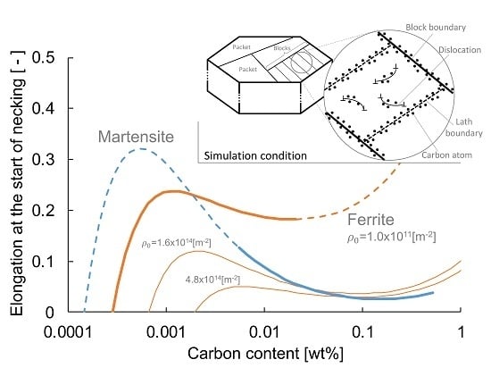
Figure 17a shows the relationship between and in martensite and ferrite with changing . Here, the same effective grain size 2.69 is used for both ferrite and martensite to remove their difference caused by grain refinement of martensite. Those curves are extended to much lower and higher regions of carbon content region in martensite and ferrite, respectively, to compare their behaviour in the same carbon content region.
This figure shows that, with increasing , in ferrite increases in the low region ( 0.002 wt%), decreases in the medium range (0.002 wt% 0.03 wt%), and then increases again in the high region (0.03 wt% ). In the low carbon region, as seen in Figure 8, dislocation generation becomes more active with increasing , which increases the hardening rate and then is higher. With the middle range of , on the other hand, dislocation recovery occurs frequently because of the large number of recovery sites generated by higher number of carbon atoms, then the hardening rate decreases, leading to lower . Furthermore, in the high region, increasing prevents thermal activation of dislocation recovery, which increases the hardening rate and again.
Figure 17a also indicates that become smaller and less sensitive against with increasing . This can be explained as the larger number of initial dislocations provides larger number of recovery sites, which lower the hardening rate even in the lower carbon region. of martensite changes in the same manner as ferrite with increasing , which depends on the same mechanism as ferrite. However, its curve is more sensitive against the carbon content than that of ferrite. For martensite, the initial dislocation density depends on the carbon content, as initial dislocations form to accommodate elastic strain fields caused by carbon atoms by forming the Cottrell atmosphere. Therefore, the carbon content controls both the initial dislocation density and dislocation propagation behaviour in martensite, which changes its drastically.
According to Figure 17b, of ferrite increases, and its increasing rate slows down with increasing . With a small grain size (∼20 ), increasing grain size decreases the Hall–Petch stress and the frequency of dislocation recovery due to the smaller number of recovery sites, leading to decreasing the stress and increasing the hardening rate, respectively, then increases. However, in the large grain size region ( 20 ), dislocation generation is less active because of less number of grain boundaries, which lowers the hardening rate and the increasing rate of . Therefore, to obtain higher elongation in DP steel, the optimal carbon content and grain size should be around 0.001 wt% and larger than 20 for ferrite, while around 0.001 wt% and larger than 5 for martensite. For both ferrite and martensite, is insensitive against , so it should be improved by reducing the carbon content, whereas should be small to keep high strength.
As for DP steels, strain localisation is caused primarily by stress incompatibilities between martensite and ferrite. It is interesting to use the model and FEM simulations to assess the role of microstructural morphology and ferrite volume fraction on strain localisation. Plastic strain distributions at necking in two DP steels are calculated by FEM, Figure 18a,b show where strain starts localising at necking in DP5 and DP2. As shown in comparison between optical microscopy images of microstructures shown in Figure 14 and Figure 18, grain boundaries in each ferrite and martensite phase are not considered explicitly for simplicity in the calculations. This is reasonable as the Taylor factor is reported to vary from 2 to 3 in BCC crystal [86,87], whilst the flow stress of martensite is 2.3 and 1.7 times as much as that of ferrite in DP2 and DP5, respectively. Furthermore, variant of newly generated ferrite grains is restricted by the K-S relationship [88,89], which reduces the difference in the Taylor factor and the stress incompatibility among adjacent grains of the same phase. Therefore, the strain incompatibility among grains of the same phase is lower than the inter-phase incompatibility and the latter is explored in this work. The figure shows that both steels exhibit deformation bands along the directions of maximum shear under tension, and strain concentration areas are seen in larger deformation bands, as observed in several studies based on the FEM [11,90,91]. According to these reports, strain concentrations are major void nucleation sites, which are caused by “large” deformation bands and it is worth exploring how deformation bands form to improve the elongation of DP steels.
In Figure 18, deformation bands are seen at oblique narrow “channels” of ferritic grains, which can be explained by their lower shear strength than their surrounding regions (i.e., martensitic grains). Thus, the variation in the ferrite volume fraction along each band is examined in DP5 and DP2. The areas presented in Figure 18 are divided into 1000 cross sections angled at for DP5 and for DP2 (deformation bands found in positive and negative angles are labeled as L and , respectively); the latter is because the bands in DP2 are angled by around due to a rotation caused by deformation in the FEM simulations. The results shown in Figure 19a,b indicate that, in DP5, most deformation bands are found near where the “peaks” of ferrite volume fraction are measured. This would indicate that having high volume fraction of neighbouring ferrite channels’ along the direction of maximum shear is a primary factor for shear localisation, although it is also observed that some ferrite peaks do not produce deformation bands. The relationship between the frequency of the peaks and deformation bands however is not clear and demands more attention.
To clarify further the relationship between ferrite channels and deformation bands, simplified microstructures were analysed. Three kinds of martensite distribution are examined: chess-board, lattice and small grains, as shown in Figure 20a. The grain size of martensite is set to the actual size in DP5 and DP2 to fix the local martensite volume fraction. In the small grain case, which is studied only in DP5, the grain size is set to 2 , 1/4 of its actual size. The distribution of ferrite volume fraction along cross sections angled at the maximum shear stress in the five microstructures are shown in Figure 20b. Comparing the chess-board and lattice cases helps to examine the effect of the amplitude in the distribution of ferrite grains, whilst the comparison between chess-board and small grains aims to clarify the effect of the frequency in the ferrite peaks. As seen in Figure 21a,b, the distribution of equivalent plastic strain at necking, no deformation bands and strain concentrations exist in the lattice pattern of DP5, in contrast to the chess-board case, which corroborates that the amplitude of ferrite volume fraction distribution strongly controls the strain bands. This is because the amplitude corresponds to the difference in strength between a ferrite channel and its surroundings. However, Figure 21a,c shows that the frequency of ferrite peaks does not affect the occurrence of strain concentrations, as both chess-board and small grains show deformation bands, although the narrower ferrite channels in the small grain case display higher strain concentrations. This can be attributed to a combined high amplitude and high frequency of ferrite peaks producing a sharp increase in the ferrite fraction on (small) localised regions. Therefore, the amplitude of ferrite distribution can be used as a primary index for the strain concentration in this kind of DP steels (with higher volume fraction of martensite), followed by the slope (product of amplitude and frequency) in ferrite volume fraction along the direction of maximum shear as secondary criterion. As real microstructures do not have such ideal periodicity and smooth variations, the standard deviation of ferrite distribution could be used instead of quantifying the slope in ferrite fraction.
On the other hand, among all cases for DP2, there is no large difference between the lattice and chess-board pattern, regardless of the difference in their amplitude. This can be explained by a smaller difference of amplitude than that in DP5, due to its higher overall ferrite volume fraction, which increases the minimum ferrite fraction in all the cross sections. Thus, the amplitude cannot be used as sole criterion to evaluate the strain concentration in such DP steels with middle volume fraction of martensite. In those steels, more ferrite–ferrite grain interactions could control strain localisation, as more deformation bands are seen in the right side of Figure 18b, where the ferrite volume fraction is higher than its left half side (70% vs. 61%). For more a detailed analysis, however, effect of grain boundaries and grain orientation among grains of the same phase should be considered, as damage has been reported to also occur near these boundaries [5,6]. This is because, after strain localisation caused by inter-phase stress incompatibility, grain boundaries allegedly cause further strain localisation that leads to localised damage. To follow such behaviour, the present model should be improved to deal with orientation distribution and ferrite–ferrite boundary interactions using methods such as crystal-plasticity FEM. Similarly, no texture was considered in the FEM calculations, as it was not reported in the experimental results from the literature. As the aim of the present work was to understand variations in plastic response of martensitic, ferritic and dual-phase steels when changing composition and grain size, it was deemed appropriate to simplify the analysis in other areas such as texture effects. Nonetheless, the influence of texture in plastic response and damage can be incorporated if the simulations are expanded into a crystal-plasticity FEM framework. This can be done in future work.
To corroborate that our analysis is not an artefact of the calculations being carried out in 2D, an additional simulation was conducted in 3D for DP5-chess-board, with similar martensite grain size and volume fraction as in Figure 21. Figure 22a shows the simulation results for the plastic equivalent strain distribution after 10% strain and Figure 22b depicts the strain distribution on the x-y plane. The microstructure consists of eight mirrored subunits, each containing two half grains of ferrite and martensite (Figure 22c). Uniaxial tension was applied along the z axis in each subunit and the three planes intersecting adjacent subunits were fixed at zero displacement; no stress/displacement conditions were imposed on the remaining faces. The deformation bands successfully appear along the sites for strain localisation in ferrite—at the corners of the ferrite grains—although the extent of plastic strain beyond the localisation point within ferrite grains is slightly lower than in Figure 21a. This is because the total area of the ferrite–martensite interface is higher in the 3D setup, which increases slightly the strength of ferrite. It is also observed that strain bands form on the z-x and y-z planes too; therefore, the probability for void formation by strain localisation should be higher compared to the 2D model. However, this effect requires a more careful analysis using realistic 3D morphologies. Nonetheless, we can confirm that the conclusions drawn from the results in Figure 20, i.e., the regions with the highest fraction of adjacent ferrite grains represent the most likely regions where deformation bands form, are in principle valid for 2D and 3D microstructures, although more detailed 3D modelling and microstructural characterisation are required to draw more accurate conclusions.
9. Conclusions
The following conclusions can be outlined:
- Modified versions of the Kocks–Mecking model are proposed, which predict the dislocation density in ferrite and martensite, considering effectiveness of carbon content and grain size on dislocation pinning and recovery. The relatively simple model was validated in single- and dual-phase steels, showing good accuracy. The models were then combined with FEM simulations to predict the deformation behaviour in dual-phase steels with different martensite volume fraction and carbon content.
- It was shown that, with increasing density of an obstacle, the dislocation generation coefficient K increases but its rate slows down with higher concentration of obstacles. This is because the strain increments produced by a dislocation interacting with that obstacle are too small due to a large energy penalty. It was demonstrated that increasing the carbon content increases both the number of dislocation recovery sites and their activation energy, and, as a result, it was found that the dislocation recovery coefficient f reaches maximum value at wt%.
- In both martensitic and ferritic steels, the relationship between uniform elongation and the carbon content reaches a maximum value in the (very) low carbon region ( < 0.01 wt%); this results from the competition between increasing dislocation generation and annihilation with increasing carbon additions. of martensite is more sensitive against carbon variations than that of ferrite, because it controls both the initial dislocation density and dislocation propagation behaviour.
- increases with increasing grain size due to decreasing the Hall–Petch stress and dislocation recovery frequency. With the grain size larger than 5 and 20 in martensite and ferrite, respectively, is insensitive to grain size variations because dislocation generation also slows down.
- Using the model results in DP steels it was predicted that optimal elongation can be reached in alloys with carbon content ∼0.01 wt%. Furthermore, its grain size should be as small as possible to maintain the ultimate tensile strength, unless the grain size of martensite and ferrite is smaller than 5 and 20 , respectively, where rapidly decreases with decreasing grain size.
- In DP steels with high volume fraction of martensite (>50%), it was found that major deformation bands causing voids occur inside “ferrite channels”, which can be detected by quantifying the ferrite volume fraction along cross sections angled at the direction of the maximum shear stress. Three simplified morphologies were studied (chess-board, lattice and small grains) to elucidate the main factors promoting the bands. Strain accumulation was attributed to a combined high amplitude and high frequency of adjacent ferrite grains, with the former being the primary contributor of deformation bands. It was concluded that, to prevent void nucleation, martensitic grains should be distributed in a lattice pattern, i.e., ferrite grains completely surrounding homogeneously distributed martensite grains.
- It was also found that major deformation bands in DP steels with medium volume fraction of martensite (∼30%) are not only promoted by a high amplitude in the ferrite peaks but also ferrite–ferrite grain interactions should play a significant role due to the much lower fraction of martensite. This implies that the level homogeneity between ferrite and martensite phases is important to prevent void nucleation in these microstructures.
Author Contributions
Conceptualisation, S.M. and E.I.G.-N.; methodology, S.M. and E.I.G.-N.; model analysis and validation, S.M.; writing draft and editing, S.M. and E.I.G.-N.; supevision, E.I.G.-N. All authors have read and agreed to the published version of the manuscript.
Funding
Part of this research was funded by the Royal Academy of Engineering.
Acknowledgments
E. I. Galindo-Nava acknowledges the Royal Academy of Engineering for his research fellowship funding via the research fellowships scheme.
Conflicts of Interest
The authors declare no conflict of interest.
References
- Takahashi, M. Sheet Steel Technology for the Last 100 Years: Progress in sheet steels in hand with the automotive industry. Tetsu-to-Hagane 2013, 100, 82–93. [Google Scholar] [CrossRef] [Green Version]
- Szewczyk, A.F.; Gurland, J. A Study of the Deformation and Fracture of a Dual-Phase Steel. Metall. Trans. A 1982, 13, 1821–1826. [Google Scholar] [CrossRef]
- Kadkhodapour, J.; Butz, A.; Ziaei-Rad, S. Mechanisms of void formation during tensile testing in a commercial, dual-phase steel. Acta Mater. 2011, 59, 1103–1125. [Google Scholar] [CrossRef]
- Roth, C.; Morgeneyer, T.; Cheng, Y.; Helfen, L.; Mohr, D. Ductile damage mechanism under shear-dominated loading: In-situ T tomography experiments on dual phase steel and localization analysis. Int. J. Plast. 2018, 109, 169–192. [Google Scholar] [CrossRef] [Green Version]
- Azuma, M.; Goutianos, S.; Hansen, N.; Winther, G.; Huang, X. Effect of hardness of martensite and ferrite on void formation in dual phase steel. Mater. Sci. Technol. 2012, 28, 1092–1100. [Google Scholar] [CrossRef]
- Archie, F.; Li, X.; Zaefferer, S. Micro-damage initiation in ferrite-martensite DP microstructures: A statistical characterization of crystallographic and chemical parameters. Mater. Sci. Eng. A 2017, 701, 302–313. [Google Scholar] [CrossRef]
- Ramazani, A.; Kazemiabnavi, S.; Larson, R. Quantification of ferrite-martensite interface in dual phase steels: A first-principles study. Acta Mater. 2016, 116, 231–237. [Google Scholar] [CrossRef]
- Sun, X.; Choi, K.; Liu, W.; Khaleel, M. Predicting failure modes and ductility of dual phase steels using plastic strain localization. Int. J. Plast. 2009, 25, 1888–1909. [Google Scholar] [CrossRef]
- Ramazani, A.; Ebrahimi, Z.; Prahl, U. Study the effect of martensite banding on the failure initiation in dual-phase steel. Comput. Mater. Sci. 2014, 87, 241–247. [Google Scholar] [CrossRef]
- Darabi, A.; Chamani, H.; Kadkhodapour, J.; Anaraki, A.; Alaie, A.; Ayatollahi, M. Micromechanical analysis of two heat-treated dual phase steels: DP800 and DP980. Mech. Mater. 2017, 110, 68–83. [Google Scholar] [CrossRef]
- Kadkhodapour, J.; Butz, A.; Ziaei-Rad, S.; Schmauder, S. A micro mechanical study on failure initiation of dual phase steels under tension using single crystal plasticity model. Int. J. Plast. 2011, 27, 1103–1125. [Google Scholar] [CrossRef]
- Kim, J.; Sung, J.; Piao, K.; Wagoner, R. The shear fracture of dual-phase steel. Int. J. Plast. 2011, 27, 1658–1676. [Google Scholar] [CrossRef]
- Ramazani, A.; Mukherjee, K.; Schwedt, A.; Goravanchi, P.; Prahl, U.; Bleck, W. Quantification of the effect of transformation-induced geometrically necessary dislocations on the flow-curve modelling of dual-phase steels. Int. J. Plast. 2013, 43, 128–152. [Google Scholar] [CrossRef]
- Ramazani, A.; Mukherjee, K.; Prahl, U.; Bleck, W. Modelling the effect of microstructural banding on the flow curve behaviour of dual-phase (DP) steels. Comput. Mater. Sci. 2012, 52, 46–54. [Google Scholar] [CrossRef]
- Ramazani, A.; Schwedt, A.; Aretz, A.; Prahl, U.; Bleck, W. Characterization and modelling of failure initiation in DP steel. Comput. Mater. Sci. 2013, 75, 35–44. [Google Scholar] [CrossRef]
- Sun, L.; Wagoner, R. Proportional and non-proportional hardening behavior of dual-phase steels. Int. J. Plast. 2013, 45, 174–187. [Google Scholar] [CrossRef]
- Roth, C.; Mohr, D. Ductile fracture experiments with locally proportional loading histories. Int. J. Plast. 2016, 79, 328–354. [Google Scholar] [CrossRef]
- Bong, H.; Limb, H.; Lee, M.; Fullwood, D.; Homer, E.; Wagoner, R. An RVE procedure for micromechanical prediction of mechanical behavior of dual-phase steel. Mater. Sci. Eng. A 2017, 695, 101–111. [Google Scholar] [CrossRef] [Green Version]
- Xu, X.P.; Needleman, A. Void nucleation by inclusion debonding in a crystal matrix. Model. Simul. Mater. Sci. Eng. 1993, 1, 111–132. [Google Scholar] [CrossRef]
- Matsuno, T.; Teodosiu, C.; Maeda, D.; Uenishi, A. Mesoscale simulation of the early evolution of ductile fracture in dual-phase steels. Int. J. Plast. 2015, 74, 17–34. [Google Scholar] [CrossRef]
- Kim, D.K.; Kim, E.Y.; Han, J.; Woo, W.; Choi, S.H. Effect of microstructural factors on void formation by ferrite/martensite interface decohesion in DP980 steel under uniaxial tension. Int. J. Plast. 2017, 94, 3–23. [Google Scholar] [CrossRef]
- Poruks, P.; Yakubtsov, I.; Boyd, J.D. Martensite-ferrite interface strength in a low-carbon bainitic steel. Scr. Mater. 2006, 54, 41–45. [Google Scholar] [CrossRef]
- Ishida, Y. Grain boundary structure and its mobility. Tetsu-to-Hagane 1984, 70, 1819. [Google Scholar] [CrossRef]
- Liao, J.; Xue, X.; Lee, M.; Barlat, F.; Vincze, G.; Pereira, A. Constitutive modeling for path-dependent behavior and its influence on twist springback. Int. J. Plast. 2017, 93, 64–88. [Google Scholar] [CrossRef]
- Yoshida, K.; Brenner, R.; Bacroix, B.; Bouvier, S. Micromechanical modeling of the work-hardening behavior of single- and dual-phase steels under two-stage loading paths. Mater. Sci. Eng. A 2011, 528, 1037–1046. [Google Scholar] [CrossRef]
- Li, X.; Roth, C.; Mohr, D. Machine-learning based temperature- and rate-dependent plasticity model: Application to analysis of fracture experiments on DP steel. Int. J. Plast. 2019, 118, 320–344. [Google Scholar] [CrossRef]
- Ayatollahi, M.; Darabi, A.; Chamani, H.; Kadkhodapour, J. 3D Micromechanical Modeling of Failure and Damage Evolution in Dual Phase Steel Based on a Real 2D Microstructure. Acta Mech. Solida Sin. 2016, 29, 95–110. [Google Scholar] [CrossRef]
- Moeini, G.; Ramazani, A.; Sundararaghavan, V.; Koenke, C. Micromechanical modeling of fatigue behavior of DP steels. Mater. Sci. Eng. A 2017, 689, 89–95. [Google Scholar] [CrossRef]
- Bond, D.M.; Zikry, M.A. Differentiating between intergranular and transgranular fracture in polycrystalline aggregates. J. Mater. Sci. 2018, 53, 5786–5798. [Google Scholar] [CrossRef]
- Cottrell, A.H. The Bakerian Lecture, 1963. Fracture. Proc. R. Soc. Lond. Ser. A Math. Phys. Sci. 1963, 276, 1–18. [Google Scholar] [CrossRef]
- Stroh, A.N. A theory of the fracture of metals. Adv. Phys. 1957, 6, 418–465. [Google Scholar] [CrossRef]
- Barlat, F.; Gracio, J.; Lee, M.; Rauch, E.; Vincze, G. An alternative to kinematic hardening in classical plasticity. Int. J. Plast. 2011, 27, 1309–1327. [Google Scholar] [CrossRef]
- Barlat, F.; Vincze, G.; Grácio, J.; Lee, M.; Rauch, E.; Tomé, C. Enhancements of homogenous anisotropic hardening model and application to mild and dual-phase steels. Int. J. Plast. 2014, 58, 201–218. [Google Scholar] [CrossRef]
- Lee, M.; Lee, J.; Gracio, J.; Vincze, G.; Rauch, E.; Barlat, F. A dislocation-based hardening model incorporated into an anisotropic hardening approach. Comput. Mater. Sci. 2013, 79, 570–583. [Google Scholar] [CrossRef]
- Carvalho Resende, T.; Bouvier, S.; Abed-Meraim, F.; Balan, T.; Sablin, S. Dislocation-based model for the prediction of the behavior of b.c.c. materials—Grain size and strain path effects. Int. J. Plast. 2013, 47, 29–48. [Google Scholar] [CrossRef] [Green Version]
- Kocks, U.; Mecking, H. Physics and phenomenology of strainhardening: The FCC case. Prog. Mater. Sci. 2003, 48, 171–273. [Google Scholar] [CrossRef]
- Haouala, S.; Segurado, J.; LLorca, J. An analysis of the influence of grain size on the strength of FCC polycrystals by means of computational homogenization. Acta Mater. 2018, 148, 72–85. [Google Scholar] [CrossRef] [Green Version]
- Okuyama, Y.; Ohashi, T. Numerical Modeling for Strain Hardening of Two-phase Alloys with Dispersion of Hard Fine Spherical Particles. Tetsu-to-Hagane 2016, 102, 396–404. [Google Scholar] [CrossRef]
- Yasuda, Y.; Shimokawa, T.; Ohashi, T.; Niiyama, T. Crystal Plasticity Analysis on Ductility of Ferrite/Cementite Multilayers: Effect of Dislocation Absorption Ability of the Hetero Interface. Tetsu-to-Hagane 2018, 105, 146–154. [Google Scholar] [CrossRef] [Green Version]
- Akama, D.; Tsuchiyama, T.; Takaki, S. Change in Dislocation Characteristics with Cold Working in Ultralow-carbon Martensitic Steel. ISIJ Int. 2016, 56, 1675–1680. [Google Scholar] [CrossRef] [Green Version]
- Aono, Y.; Kitajima, K.; Kuramoto, E. Thermally activated slip deformation of FeNi alloy single crystals in the temperature range of 4.2 K to 300 K. Scr. Metall. 1981, 15, 275–279. [Google Scholar] [CrossRef]
- Jo, K.R.; Seo, E.J.; Hand Sulistiyo, D.; Kim, J.K.; Kim, S.W.; De Cooman, B.C. On the plasticity mechanisms of lath martensitic steel. Mater. Sci. Eng. A 2017, 704, 252–261. [Google Scholar] [CrossRef]
- Kinney, C.C.; Pytlewski, K.R.; Khachaturyan, A.G.; Morris, J.W. The microstructure of lath martensite in quenched 9Ni steel. Acta Mater. 2014, 69, 372–385. [Google Scholar] [CrossRef]
- Morito, S.; Yoshida, H.; Maki, T.; Huang, X. Effect of block size on the strength of lath martensite in low carbon steels. Mater. Sci. Eng. A 2006, 438–440, 237–240. [Google Scholar] [CrossRef]
- Galindo-Nava, E.I.; Rivera-Díaz-Del-Castillo, P.E. A model for the microstructure behaviour and strength evolution in lath martensite. Acta Mater. 2015, 98, 81–93. [Google Scholar] [CrossRef] [Green Version]
- Queyreau, S.; Monnet, G.; Devincre, B. Orowan strengthening and forest hardening superposition examined by dislocation dynamics simulations. Acta Mater. 2010, 58, 5586–5595. [Google Scholar] [CrossRef]
- Kim, B.; Boucard, E.; Sourmail, T.; San Martín, D.; Gey, N.; Rivera-Díaz-Del-Castillo, P.E. The influence of silicon in tempered martensite: Understanding the microstructure-properties relationship in 0.5–0.6 wt.% C steels. Acta Mater. 2014, 68, 169–178. [Google Scholar] [CrossRef]
- Kato, M. Nyumon Teni-ron [Fundamentals of Dislocations], 6th ed.; Shokabo: Tokyo, Japan, 2007; Chapter 4; p. 43. [Google Scholar]
- Hutchinson, B.; Hagström, J.; Karlsson, O.; Lindell, D.; Tornberg, M.; Lindberg, F.; Thuvander, M. Microstructures and hardness of as-quenched martensites (0.1–0.5%C). Acta Mater. 2011, 59, 5845–5858. [Google Scholar] [CrossRef]
- Song, W.; Drouven, C.; Galindo-Nava, E. Carbon redistribution in martensite in a high-C steel: Atomic-scale characterization and modelling. Metals 2018, 8, 577. [Google Scholar] [CrossRef] [Green Version]
- Cottrell, A.H.; Bilby, B.A. Dislocation Theory of Yielding and Strain Ageing of Iron. Proc. Phys. Soc. Sect. A 1949, 62, 49. [Google Scholar] [CrossRef]
- Cochardt, A.W.; Schoek, G.; Wiedersich, H. Interaction between dislocations and interstitial atoms in body-centered cubic metals. Acta Metall. 1955, 3, 533–537. [Google Scholar] [CrossRef]
- Nabarro, F.; Basinski, Z.; Holt, D. The plasticity of pure single crystals. Adv. Phys. 1964, 13, 193–323. [Google Scholar] [CrossRef]
- Caillard, D.; Legros, M.; Couret, A. Extrinsic obstacles and loop formation in deformed metals and alloys. Philos. Mag. 2013, 93, 203–221. [Google Scholar] [CrossRef]
- Hafez Haghighat, S.M.; Schäublin, R. Obstacle strength of binary junction due to dislocation dipole formation: An in-situ transmission electron microscopy study. J. Nucl. Mater. 2015, 465, 648–652. [Google Scholar] [CrossRef]
- Low, J.R.; Turkalo, A.M. Slip band structure and dislocation multiplication in silicon-iron crystals. Acta Metall. 1962, 10, 215–227. [Google Scholar] [CrossRef]
- Washburn, J.; Groves, G.W.; Kelly, A.; Williamson, G.K. Electron microscope observations of deformed magnesium oxide. Philos. Mag. 1960, 5, 991–999. [Google Scholar] [CrossRef]
- Anderson, P.M.; Hirth, J.P.; Lothe, J. Theory of Dislocations, 3rd ed.; Cambridge University Press: Cambridge, UK, 2017. [Google Scholar]
- Friedman, L.; Chrzan, D. Continuum analysis of dislocation pile-ups: Influence of sources. Philos. Mag. A 1998, 77, 1185–1204. [Google Scholar] [CrossRef]
- Kocks, U.F.; Argon, A.S.; Ashby, M.F. Thermodynamics and Kinetics of Slip; Pergamon Press: London, UK, 1975. [Google Scholar]
- Ono, K.; Sommer, A.W. Peierls-Nabarro hardening in the presence of point obstacles. Metall. Trans. 1970, 1, 877–884. [Google Scholar] [CrossRef]
- Adlakha, I.; Solanki, K.N. Critical assessment of hydrogen effects on the slip transmission across grain boundaries in α-Fe. Proc. R. Soc. A Math. Phys. Eng. Sci. 2016, 472. [Google Scholar] [CrossRef] [Green Version]
- Mondal, D.K.; Dey, R.M. Effect of grain size on the microstructure and mechanical properties of a CMnV dual-phase steel. Mater. Sci. Eng. A 1992, 149, 173–181. [Google Scholar] [CrossRef]
- Ashrafi, H.; Sadeghzade, S.; Emadi, R.; Shamanian, M. Influence of Heat Treatment Schedule on the Tensile Properties and Wear Behavior of Dual Phase Steels. Steel Res. Int. 2017, 88, 1600213. [Google Scholar] [CrossRef]
- Schneider, C.A.; Rasband, W.S.; Eliceiri, K.W. NIH Image to ImageJ: 25 years of image analysis. Nat. Methods 2012, 9, 671–675. [Google Scholar] [CrossRef] [PubMed]
- Clarke, A.J.; Miller, M.K.; Field, R.D.; Coughlin, D.R.; Gibbs, P.J.; Clarke, K.D.; Alexander, D.J.; Powers, K.A.; Papin, P.A.; Krauss, G. Atomic and nanoscale chemical and structural changes in quenched and tempered 4340 steel. Acta Mater. 2014, 77, 17–27. [Google Scholar] [CrossRef]
- Sherman, D.H.; Cross, S.M.; Kim, S.; Grandjean, F.; Long, G.J.; Miller, M.K. Characterization of the Carbon and Retained Austenite Distributions in Martensitic Medium Carbon, High Silicon Steel. Metall. Mater. Trans. A 2007, 38, 1698–1711. [Google Scholar] [CrossRef]
- Pereloma, E.V.; Timokhina, I.B.; Jonas, J.J.; Miller, M.K. Fine-scale microstructural investigations of warm rolled low-carbon steels with and without Cr, P, and B additions. Acta Mater. 2006, 54, 4539–4551. [Google Scholar] [CrossRef]
- Maruyama, N.; Takahashi, M. Segregation and Precipitation of Carbon in the Vicinity of Dislocations during Strain Aging in Low Carbon Steels. Tetsu-to-Hagane 2009, 93, 506–512. [Google Scholar] [CrossRef] [Green Version]
- Ratanaphan, S.; Olmsted, D.; Bulatov, V.; Holm, E.; Rollett, A.; Rohrer, G. Grain boundary energies in body-centered cubic metals. Acta Mater. 2015, 88, 346–354. [Google Scholar] [CrossRef] [Green Version]
- Hanamura, T.; Torizuka, S.; Tamura, S.; Enokida, S.; Takech, H. Effect of Austenite Grain Size on the Mechanical Properties in Air-Cooled 0.1C-5Mn Martensitic Steel. Mater. Sci. Forum 2014, 783–786, 1027–1032. [Google Scholar] [CrossRef]
- Huang, F.; Yang, J.; Guo, Z.; Chen, S.; Rong, Y.; Chen, N. Effect of Partitioning Treatment on the Mechanical Property of Fe-0.19C-1.47Mn-1.50Si Steel with Refined Martensitic Microstructure. Metall. Mater. Trans. A Phys. Metall. Mater. Sci. 2016, 47, 1072–1082. [Google Scholar] [CrossRef]
- Li, S.; Zhu, G.; Kang, Y. Effect of substructure on mechanical properties and fracture behavior of lath martensite in 0.1C-1.1Si-1.7Mn steel. J. Alloys Compd. 2016, 675, 104–115. [Google Scholar] [CrossRef]
- Xia, S.; Zhang, F.; Zhang, C.; Yang, Z. Mechanical Properties and Microstructures of a Novel Low-carbon High-silicon Martensitic Steel. ISIJ Int. 2017, 57, 558–563. [Google Scholar] [CrossRef] [Green Version]
- Saeglitz, M.; Krauss, G. Deformation, Fracture, and Mechanical Properties of Low- Temperature-Tempered Martensite in SAE 43xx Steels. Metall. Mater. Trans. A 1997, 28A, 377–387. [Google Scholar] [CrossRef]
- Rana, R.; Bleck, W.; Singh, S.; Mohanty, O. Laboratory investigations on copper-alloyed interstitial free steel - Part II: Effect of colling temperature. Steel Res. Int. 2007, 78, 622–630. [Google Scholar] [CrossRef]
- Nakada, N.; Fujihara, M.; Tsuchiyama, T.; Takaki, S. Effect of Phosphorus on Hall-Petch Coefficient in Ferritic Steel. ISIJ Int. 2011, 51, 1169–1173. [Google Scholar] [CrossRef] [Green Version]
- Nicaise, N.; Berbenni, S.; Wagner, F.; Berveiller, M.; Lemoine, X. Coupled effects of grain size distributions and crystallographic textures on the plastic behaviour of if steels. Int. J. Plast. 2011, 27, 232–249. [Google Scholar] [CrossRef]
- Zhao, Y.; Song, S. An experiment-based model of combined hardening and non-hardening embrittlement in an interstitial free steel. Mater. Sci. Eng. A 2018, 721, 189–199. [Google Scholar] [CrossRef]
- Das, A.; Biswas, P.; Tarafder, S.; Chakrabarti, D.; Sivaprasad, S. Effect of Strengthening Mechanism on Strain-Rate Related Tensile Properties of Low-Carbon Sheet Steels for Automotive Application. J. Mater. Eng. Perform. 2018, 27, 3709–3722. [Google Scholar] [CrossRef]
- Li, J.; Weng, G.J.; Chen, S.; Wu, X. On strain hardening mechanism in gradient nanostructures. Int. J. Plast. 2017, 88, 89–107. [Google Scholar] [CrossRef] [Green Version]
- Byun, T.S.; Kim, I.S. Tensile properties and inhomogeneous deformation of ferrite-martensite dual-phase steels. J. Mater. Sci. 1993, 28, 2923–2932. [Google Scholar] [CrossRef]
- Speich, G.R.; Leslie, W.C. Tempering of steel. Metall. Trans. 1972, 3, 1043–1054. [Google Scholar] [CrossRef]
- Bouaziz, O.; Buessler, P. Iso-work Increment Assumption for Heterogeneous Material Behaviour Modelling. Adv. Eng. Mater. 2004, 6, 79–83. [Google Scholar] [CrossRef]
- Rivera-Díaz-del Castillo, P.E.J.; Hayashi, K.; Galindo-Nava, E.I. Computational design of nanostructured steels employing irreversible thermodynamics. Mater. Sci. Technol. 2013, 29, 1206–1211. [Google Scholar] [CrossRef]
- Li, S.; Guo, C.; Hao, L.; Kang, Y.; An, Y. In-situ EBSD study of deformation behaviour of 600 MPa grade dual phase steel during uniaxial tensile tests. Mater. Sci. Eng. A 2019, 759, 624–632. [Google Scholar] [CrossRef]
- El Shawish, S.; Hure, J. Intergranular normal stress distributions in untextured polycrystalline aggregates. Eur. J. Mech. A/Solids 2018, 72, 354–373. [Google Scholar] [CrossRef] [Green Version]
- Ameyama, K.; Maki, T.; Tamura, I. Morphology and Crystallography of the Precipitation of Austenite at Ferrite Grain Boundaries in Two-Phase Stainless Steel. J. Jpn. Inst. Met. 1986, 50, 602–611. [Google Scholar] [CrossRef]
- Furuhara, T.; Takagi, S.; Watanabe, H.; Maki, T. Crystallography of grain boundary α precipitates in a β titanium alloy. Metall. Mater. Trans. A 1996, 27, 1635–1646. [Google Scholar] [CrossRef]
- Choi, S.H.; Kim, E.Y.; Woo, W.; Han, S.; Kwak, J. The effect of crystallographic orientation on the micromechanical deformation and failure behaviors of DP980 steel during uniaxial tension. Int. J. Plast. 2013, 45, 85–102. [Google Scholar] [CrossRef]
- Jafari, M.; Ziaei-Rad, S.; Saeidi, N.; Jamshidian, M. Micromechanical analysis of martensite distribution on strain localization in dual phase steels by scanning electron microscopy and crystal plasticity simulation. Mater. Sci. Eng. A 2016, 670, 57–67. [Google Scholar] [CrossRef]
Figure 1.
(a) Multi layered structure and interior of martensite. Schematic images of (b) dislocation density increase by pinning obstacles and (c) increase in glide distance at a constant dislocation density.
Figure 1.
(a) Multi layered structure and interior of martensite. Schematic images of (b) dislocation density increase by pinning obstacles and (c) increase in glide distance at a constant dislocation density.

Figure 2.
Schematic illustration of dislocation interaction with carbon atoms.

Figure 3.
Schematic illustration of the process of a gliding dislocation to overcome a dislocation forest: (a) intersection of forest dislocations; (b) glide with jogs; (c) pinch-off of dipoles; and (d) glide without jogs.
Figure 3.
Schematic illustration of the process of a gliding dislocation to overcome a dislocation forest: (a) intersection of forest dislocations; (b) glide with jogs; (c) pinch-off of dipoles; and (d) glide without jogs.

Figure 4.
Schematic representation of dislocation pile-up at a grain boundary.

Figure 5.
Schematic illustration of the volume and the area of atoms involved in an interaction with: (a) dislocation; and (b) grain boundary.
Figure 5.
Schematic illustration of the volume and the area of atoms involved in an interaction with: (a) dislocation; and (b) grain boundary.

Figure 6.
Schematic illustration of mesh and morphology used in FEM for DP5.

Figure 7.
Model-Experiment plot for: (a) K; (b) f; and (c) .

Figure 8.
Effectiveness of on: (a) K; and (b) f.

Figure 9.
Effectiveness of on: (a) K; and (b) f.

Figure 10.
Model-Experiment plot of the yield strength.

Figure 11.
Results of stress–strain curve prediction (Martensitic steels) for several values of: (a) ; and (b) .
Figure 11.
Results of stress–strain curve prediction (Martensitic steels) for several values of: (a) ; and (b) .

Figure 12.
Stress–strain curve prediction for various of Ferritic steels.

Figure 13.
Stress–strain curve predictions for DP steels which martensite volume fraction is: (a) less than 40%; (b) 40% to 50%; and (c) larger than 50%, respectively.
Figure 13.
Stress–strain curve predictions for DP steels which martensite volume fraction is: (a) less than 40%; (b) 40% to 50%; and (c) larger than 50%, respectively.

Figure 14.
Optical micrographs of (a) DP5, reproduced from [63], with permission from Elsevier, 1992, and (b) DP2, reproduced from [64], with permission from John Wiley and Sons, 2016, respectively, where the areas indicated by red broken lines were used in FEM simulations.

Figure 15.
Comparison of stress–strain curve prediction between iso-work and FEM in DP5 and DP2.

Figure 16.
against: (a) ; and (b) .

Figure 17.
against (a) and (b) in ferrite and martensite.

Figure 18.
Distributions of plastic equivalent strain of ferrite at the start of necking in: (a) DP5; and (b) DP2.
Figure 18.
Distributions of plastic equivalent strain of ferrite at the start of necking in: (a) DP5; and (b) DP2.

Figure 19.
Ferrite volume fraction in each cross section: (a) from upper left to lower right in DP5; (b) from upper right to lower left in DP5; (c) from upper left to lower right in DP2; and (d) from upper right to lower left in DP2.
Figure 19.
Ferrite volume fraction in each cross section: (a) from upper left to lower right in DP5; (b) from upper right to lower left in DP5; (c) from upper left to lower right in DP2; and (d) from upper right to lower left in DP2.

Figure 20.
(a) Schematic images of three simplified microstructures; and (b) ferrite volume fraction of each cross section in those microstructures.
Figure 20.
(a) Schematic images of three simplified microstructures; and (b) ferrite volume fraction of each cross section in those microstructures.

Figure 21.
Distributions of plastic equivalent strain in simplified microstructures: (a) DP5-chess-board; (b) DP5-lattice; (c) DP5-chess-board (small grain); (d) DP2-chess-board; and (e) DP2-lattice, respectively.
Figure 21.
Distributions of plastic equivalent strain in simplified microstructures: (a) DP5-chess-board; (b) DP5-lattice; (c) DP5-chess-board (small grain); (d) DP2-chess-board; and (e) DP2-lattice, respectively.

Figure 22.
Plastic equivalent strain distribution in DP5-chess-board assuming (a) 3D morphology and its (b) respective distribution on the x-y plane. (c) Microstructure and load configuration used for the simulation.
Figure 22.
Plastic equivalent strain distribution in DP5-chess-board assuming (a) 3D morphology and its (b) respective distribution on the x-y plane. (c) Microstructure and load configuration used for the simulation.


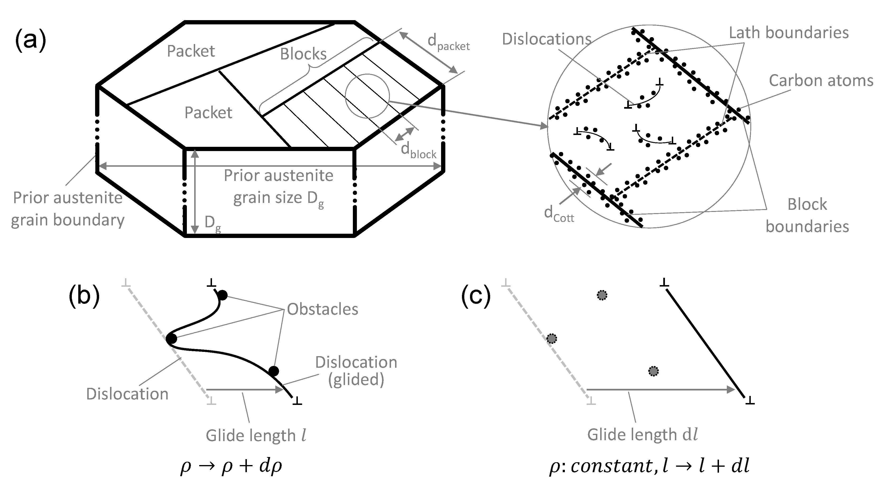
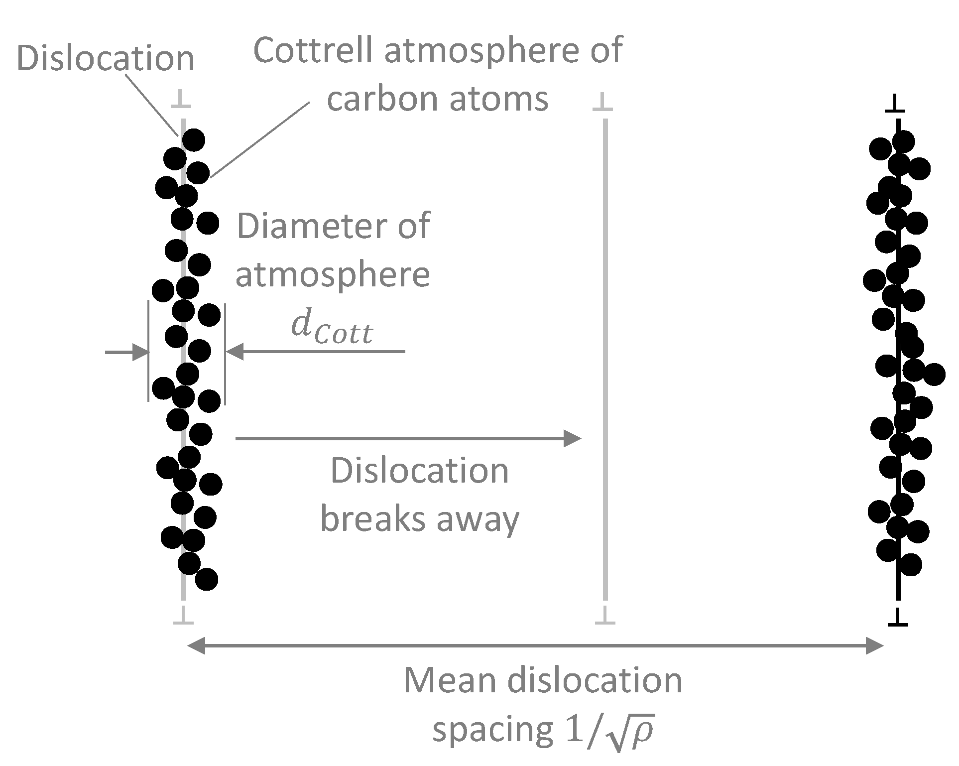
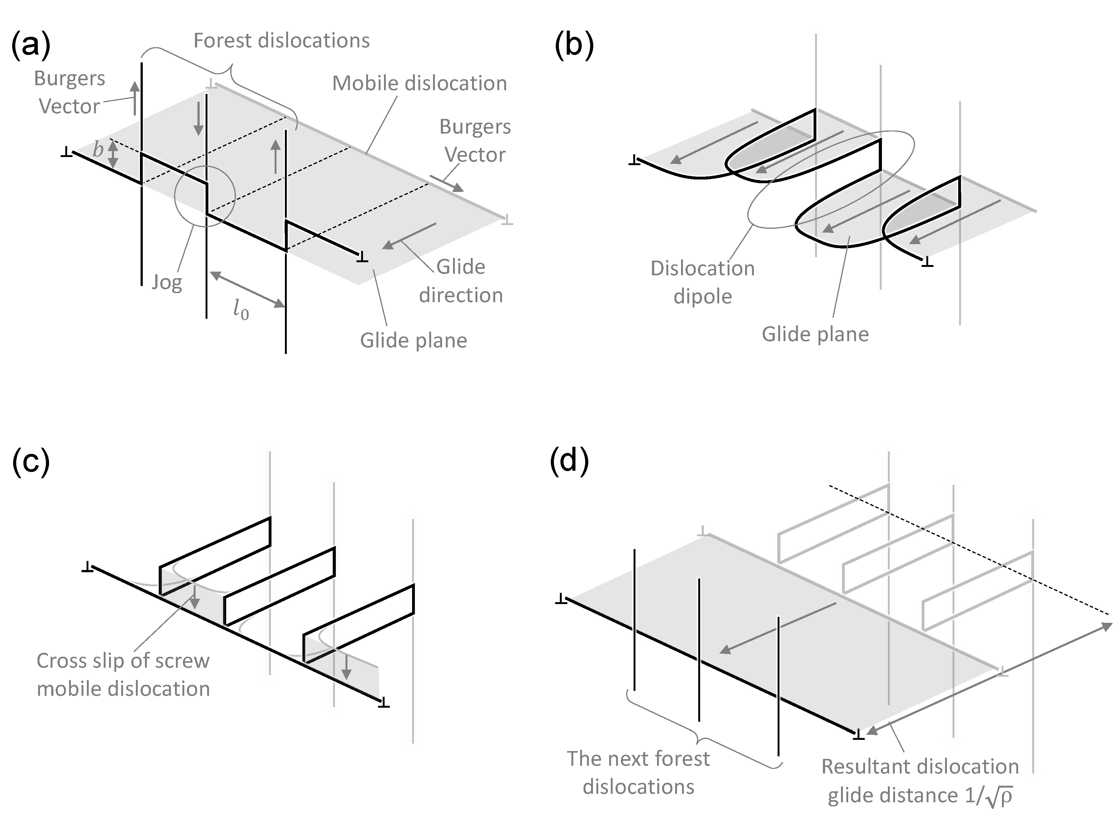
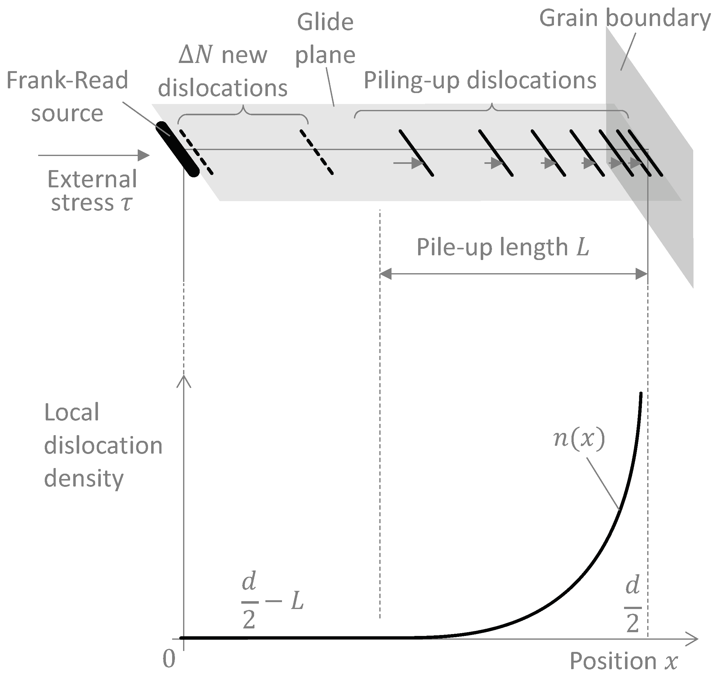
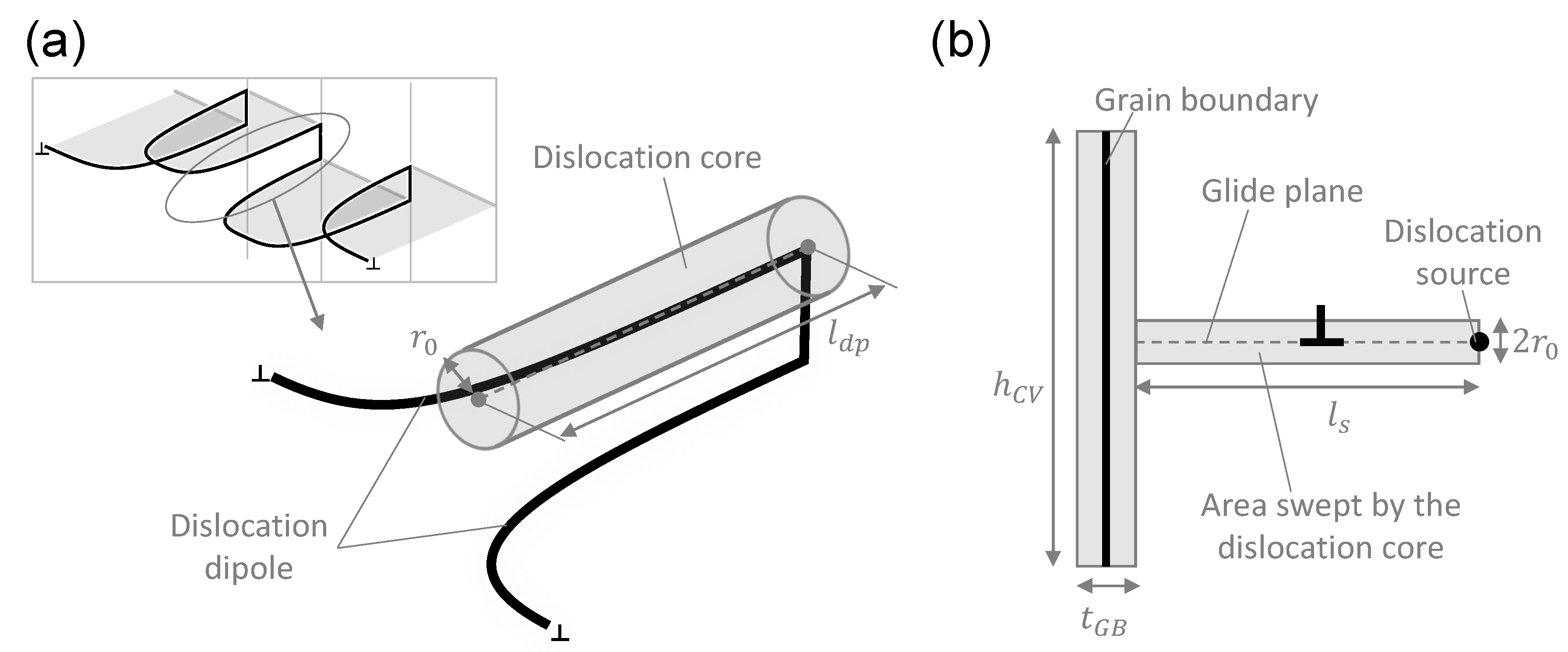
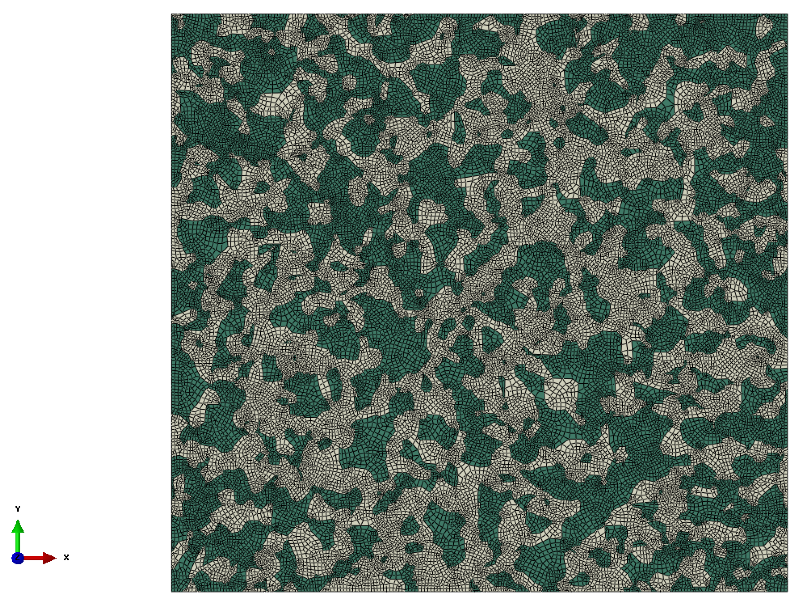
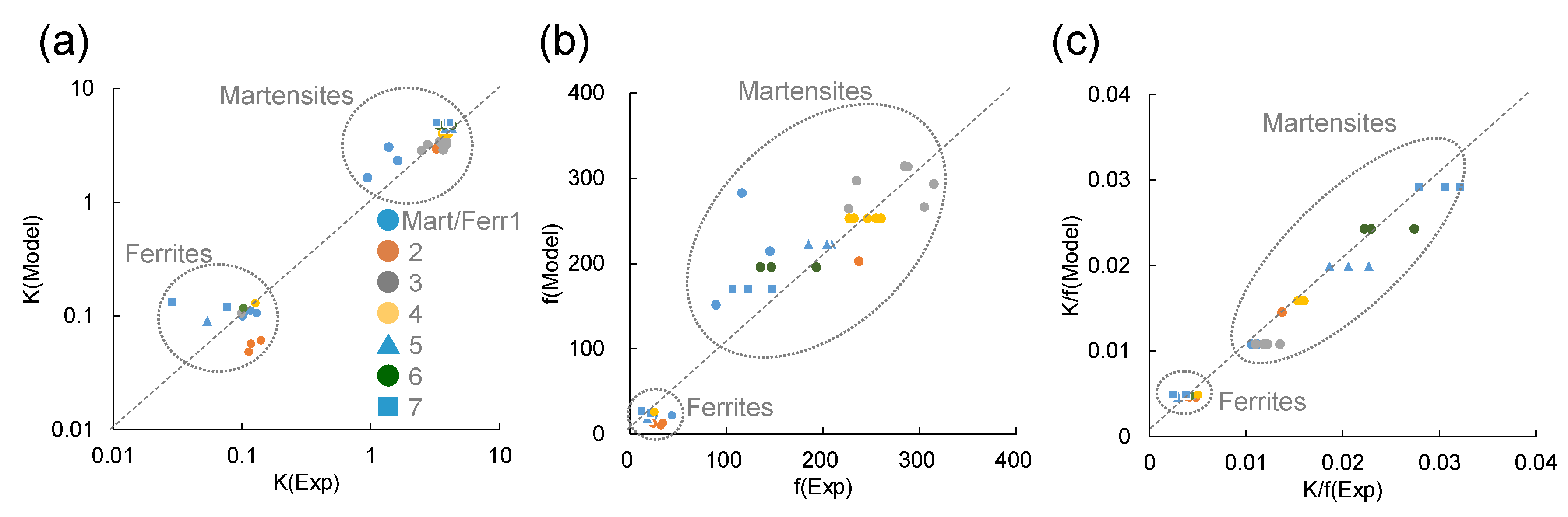
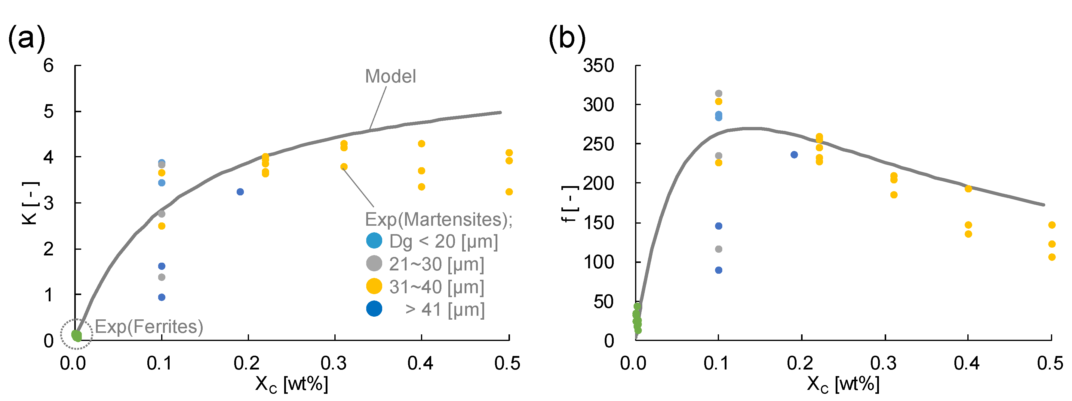
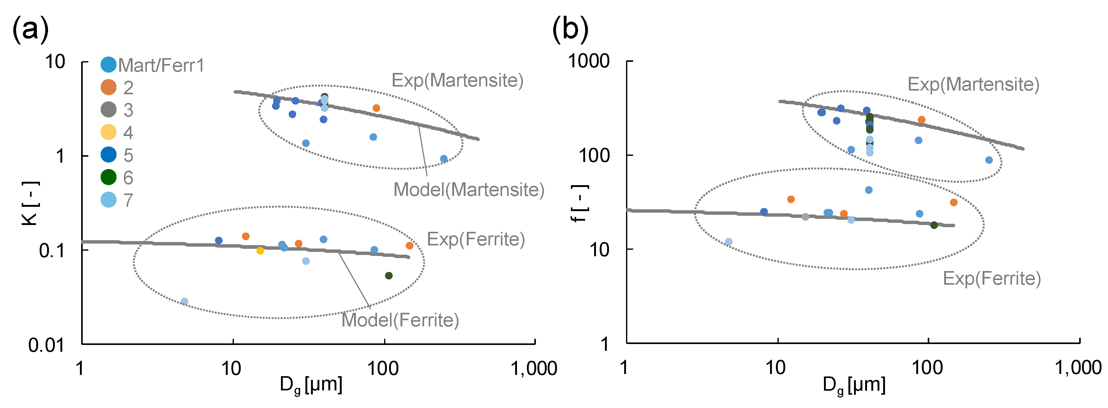
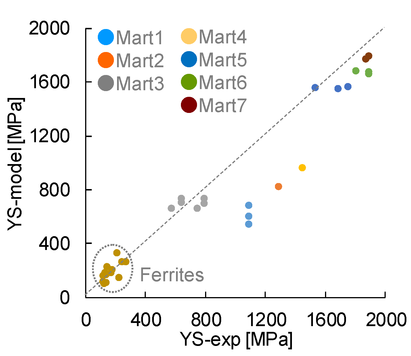
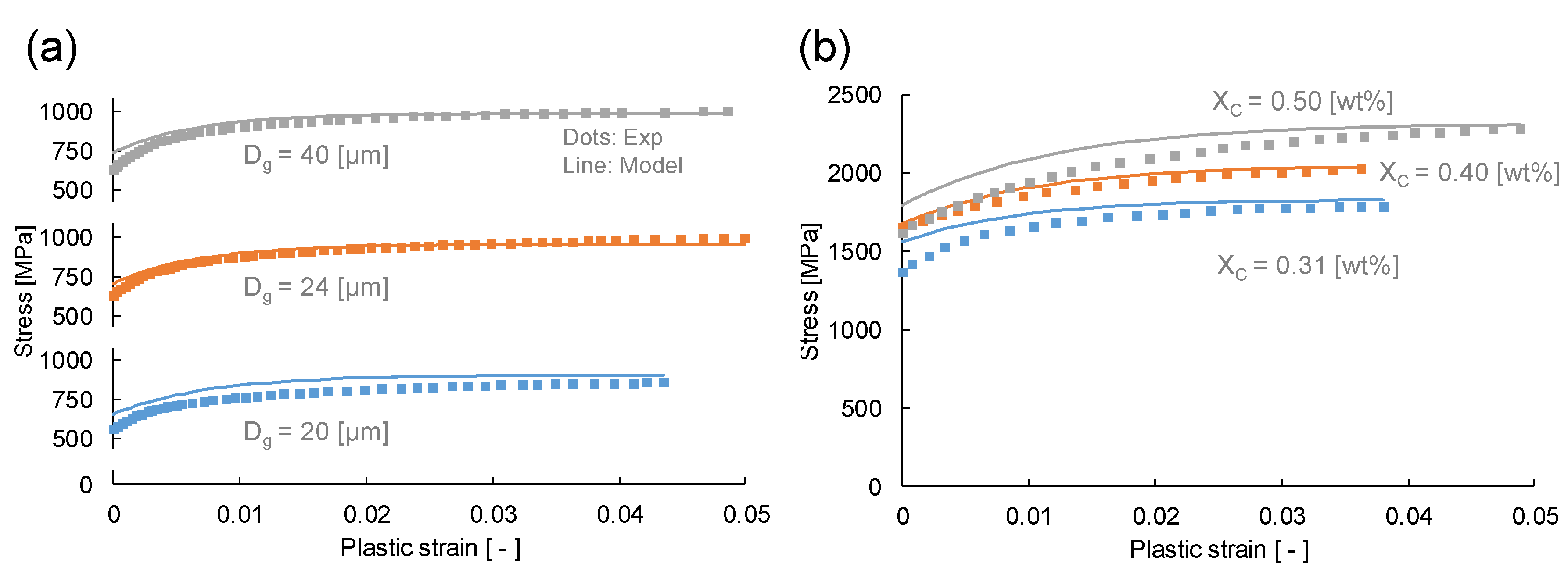
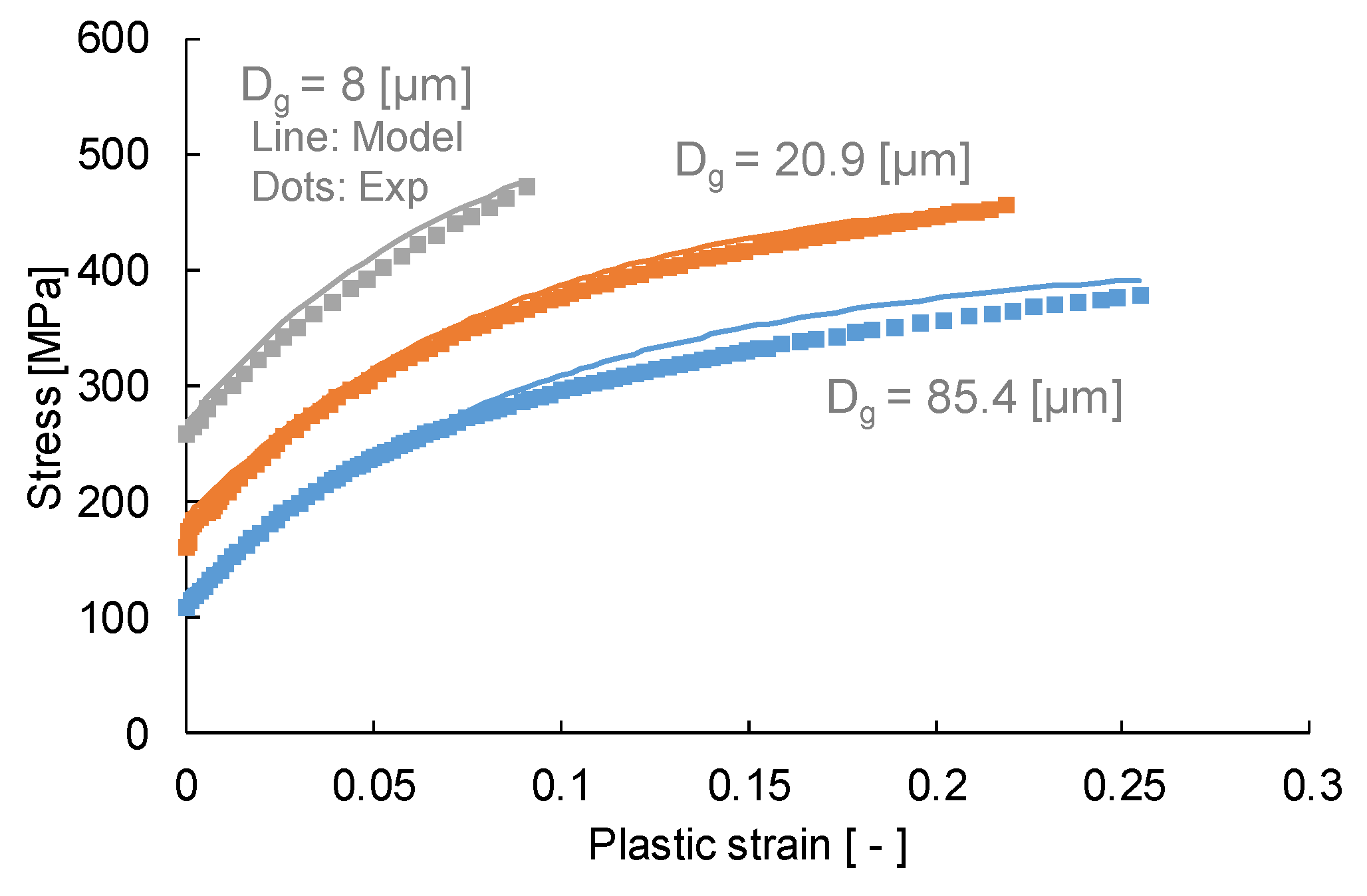
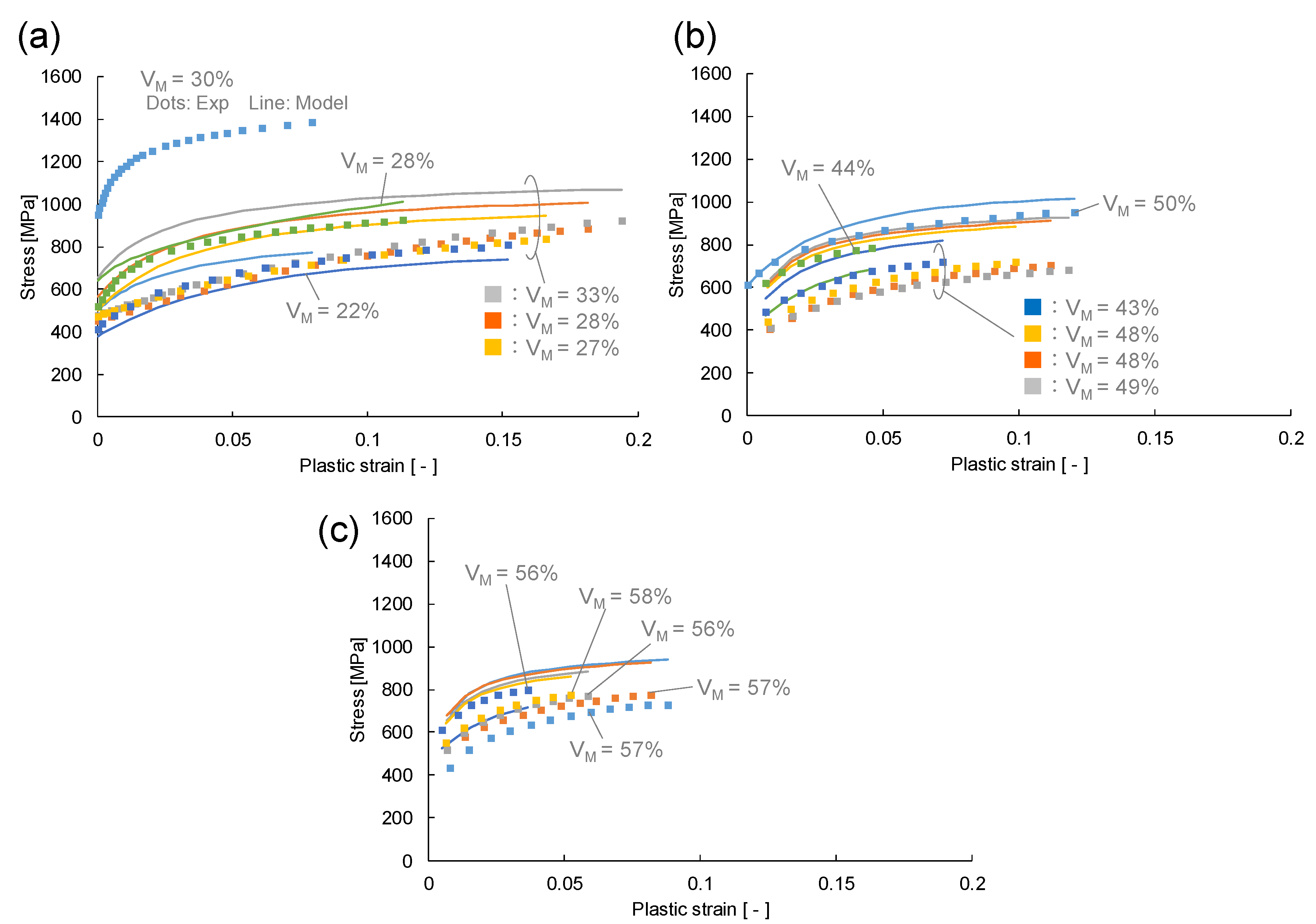
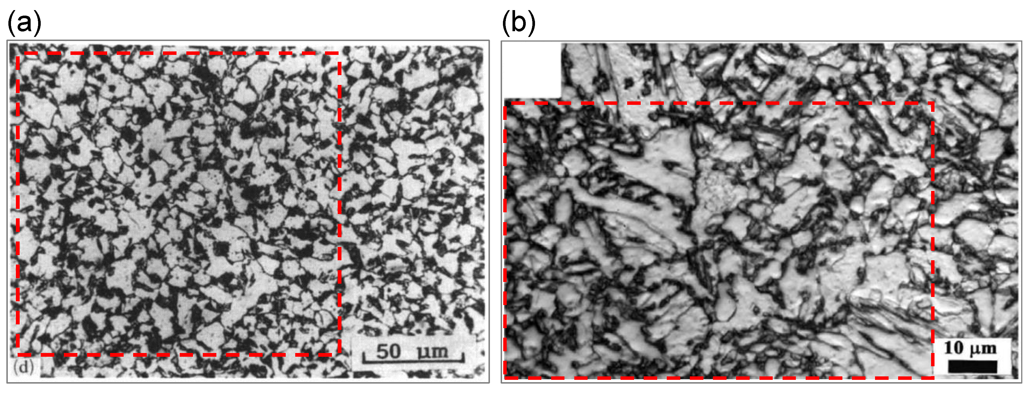
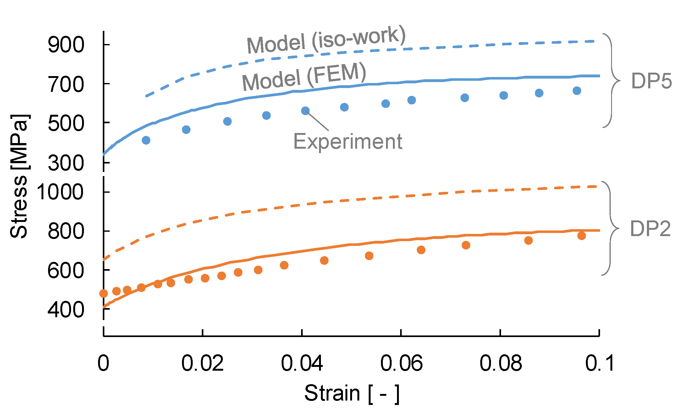
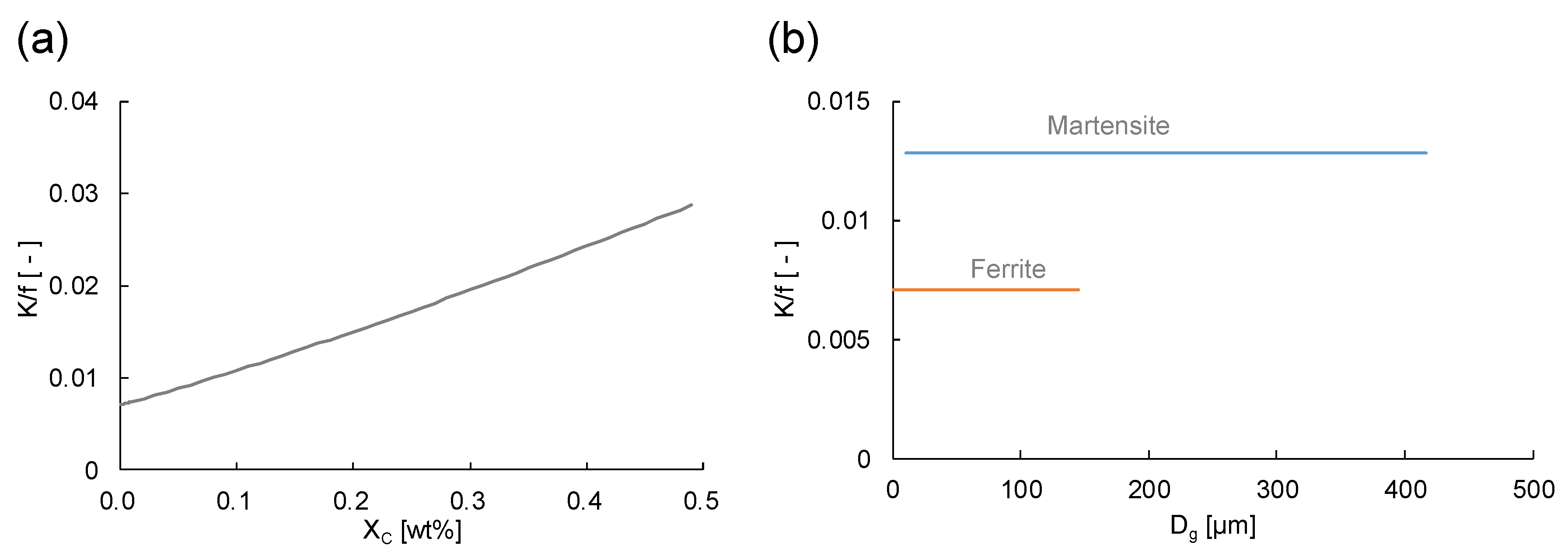
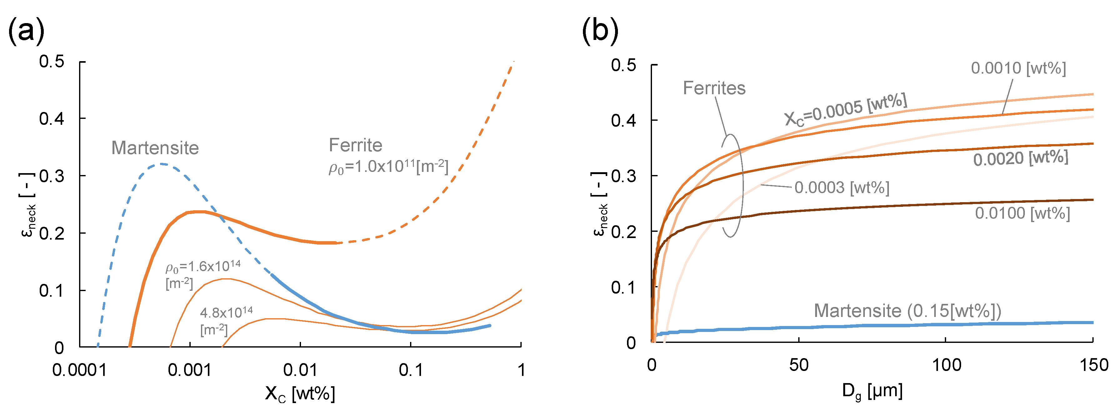
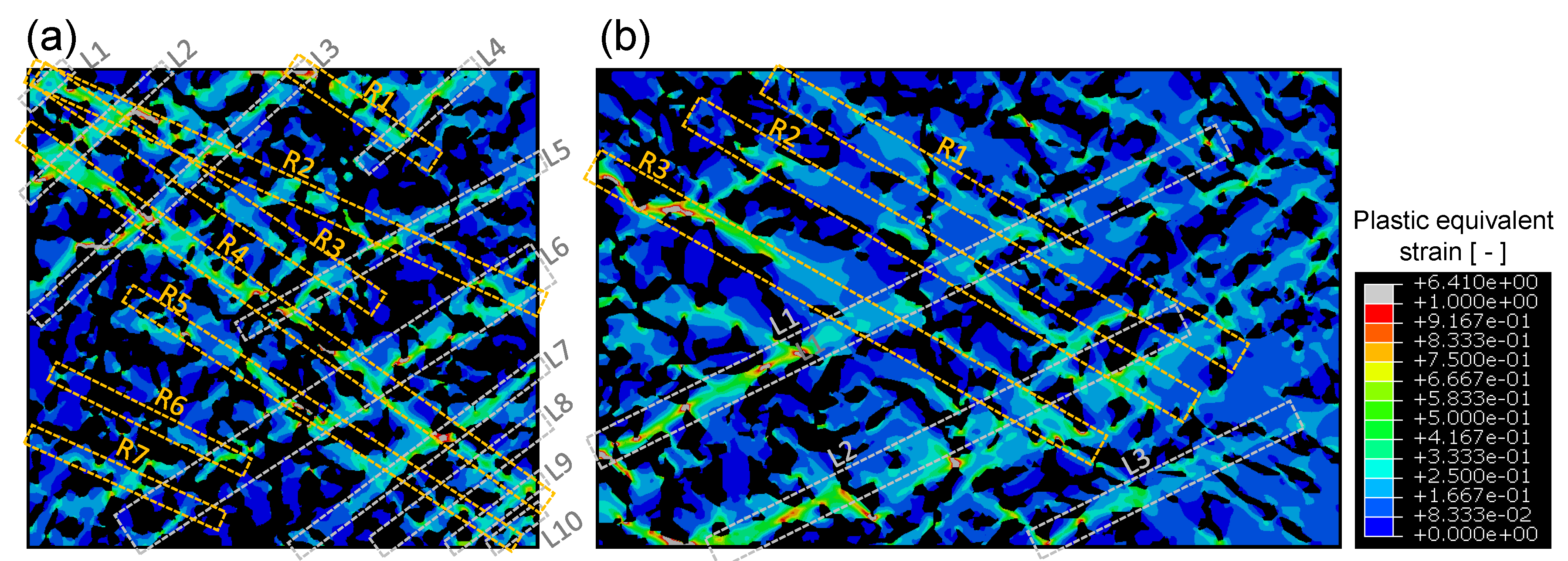
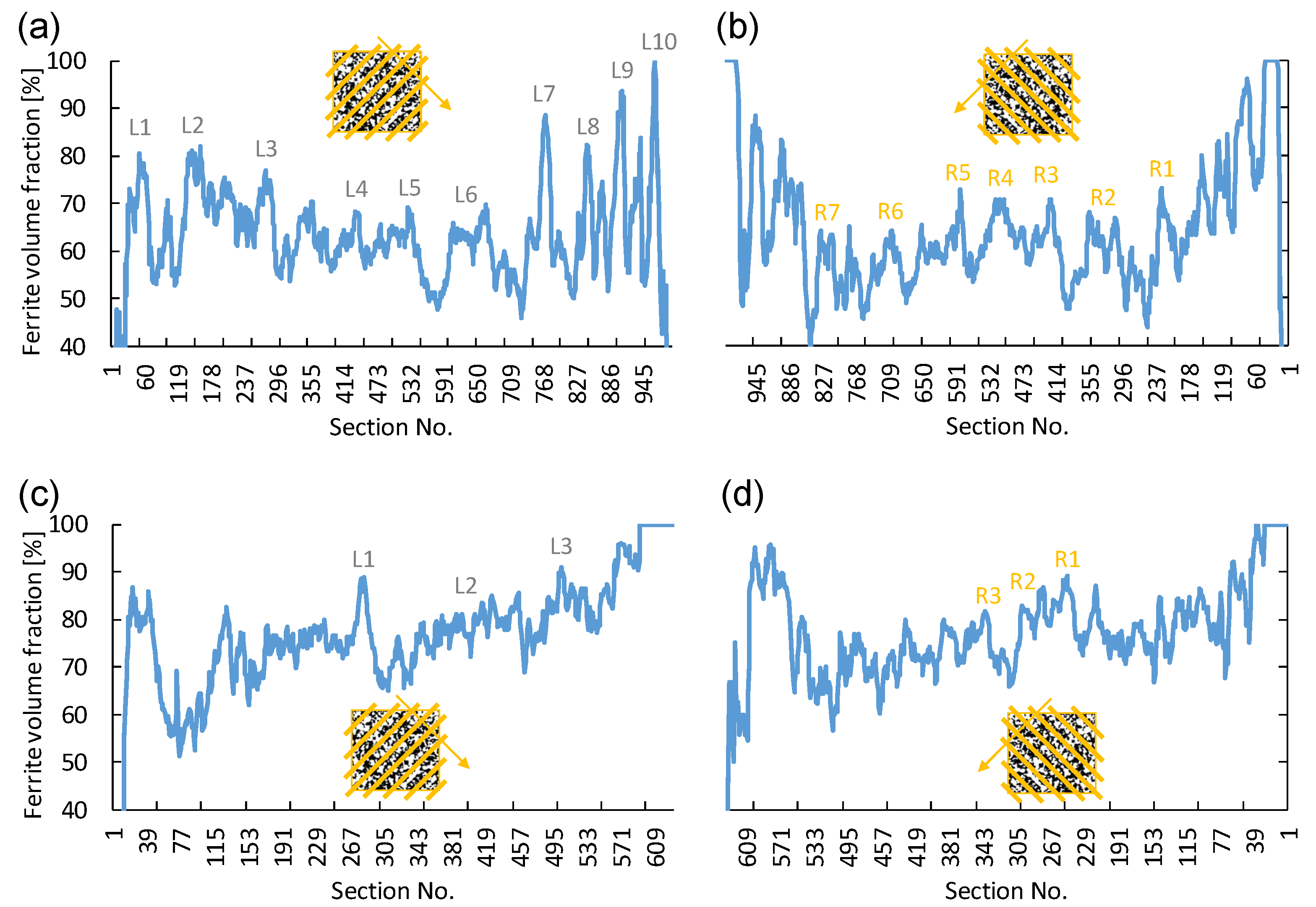
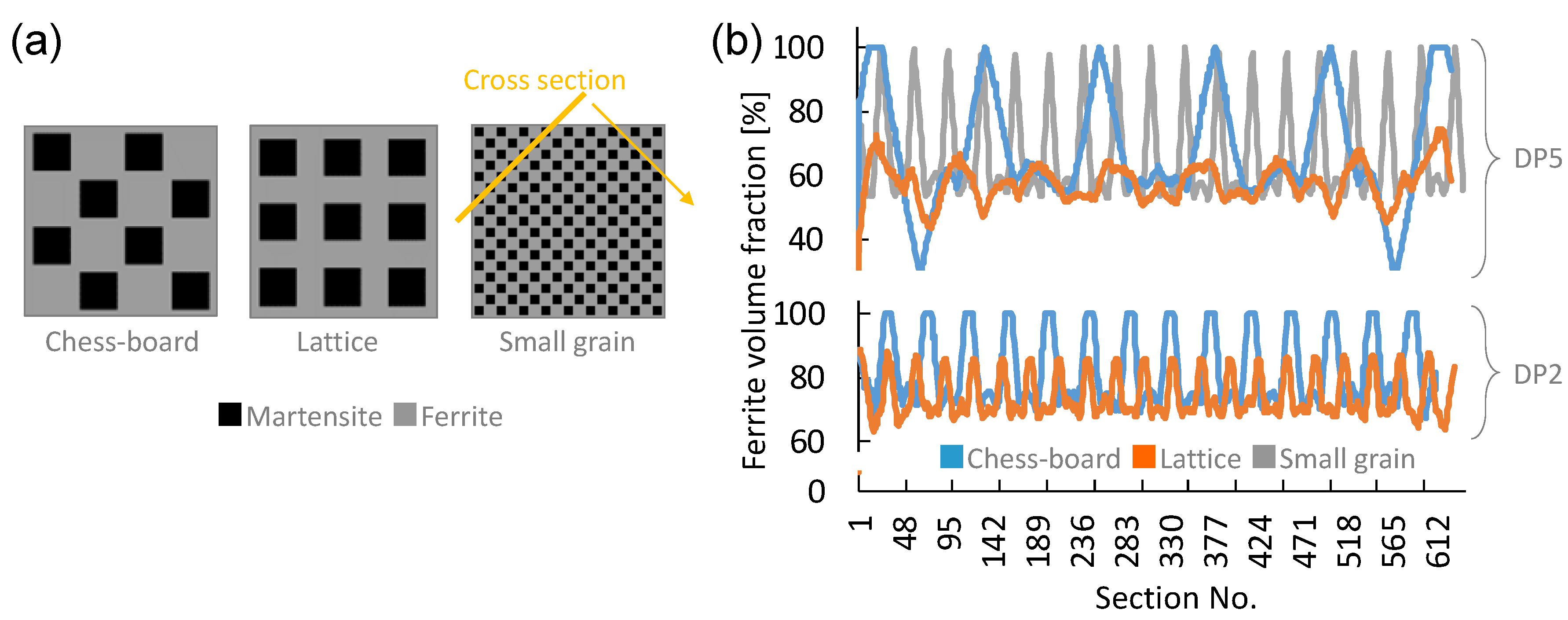
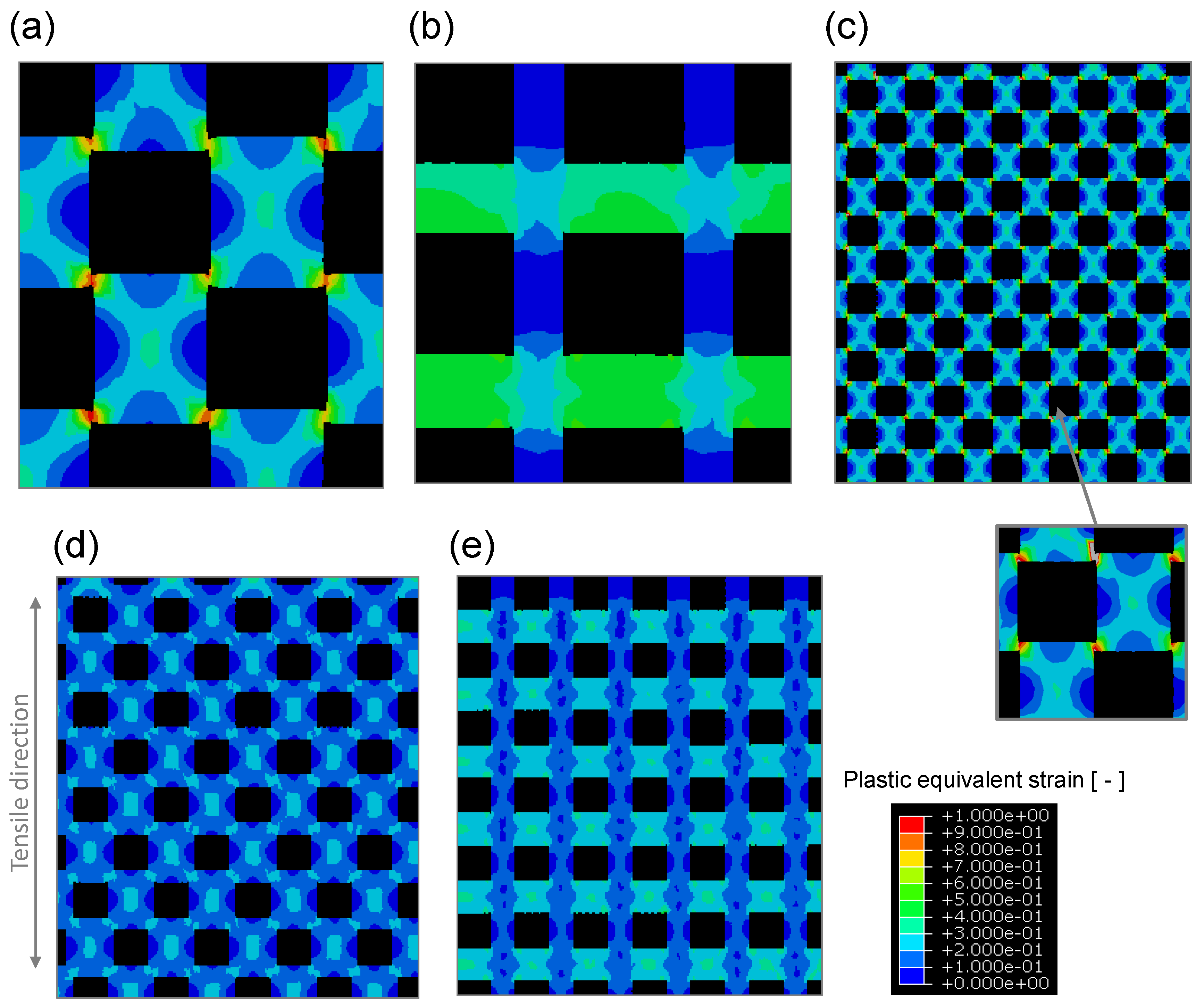
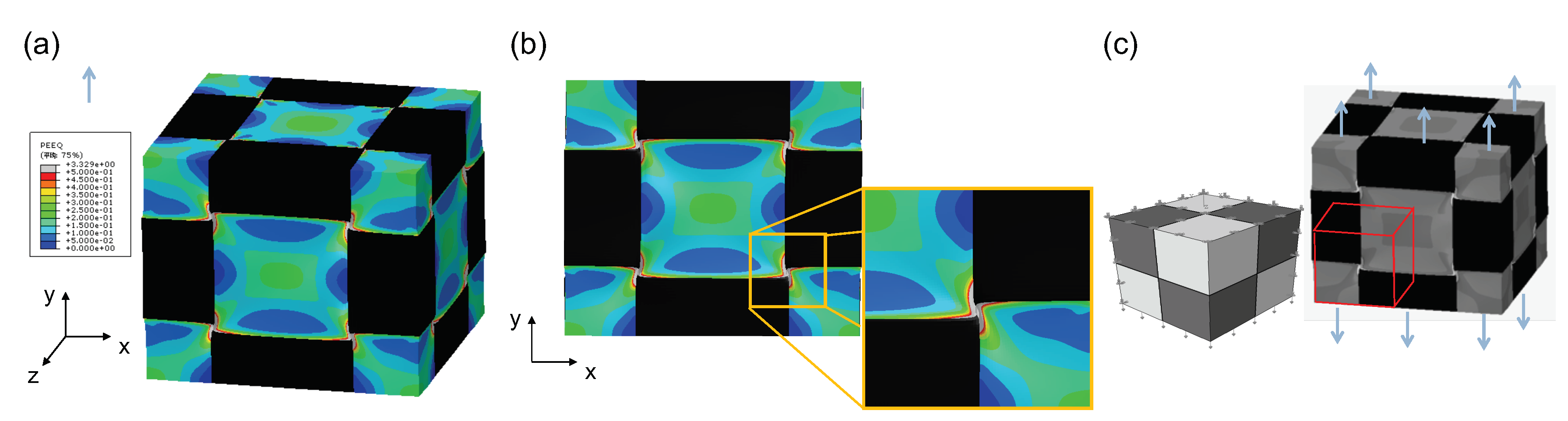
Table 1.
Parameters for prediction.
| Parameter | Value | Unit | Ref. |
|---|---|---|---|
| - | 0.25 | [48] | |
| a | Å | 2.88 | [45] |
| Å | 5 | [48] | |
| - | 0.38 | [52] | |
| - | [52] | ||
| 14 | [42] | ||
| (martensite) | - | 2.3 | [42,66,67] |
| (ferrite) | - | 9.34 | [68,69] |
| (martensite) | [40] | ||
| (ferrite) | [48] | ||
| 100 | [55] | ||
| - | 0.12 | [40] | |
| (martensite) | [62,70] | ||
| (ferrite) | [62,70] | ||
| [36] | |||
| Å | 300 | [62] | |
| Å | 50 | [62] | |
| Å | 8.58 | [62] | |
| MPa | 50 | [45] |
Table 2.
Parameters and chemical compositions (in wt%) of martensitic steels.
| Steel | T [K] | [s] | [m] | C | Si | Mn | P | S | Ref. |
|---|---|---|---|---|---|---|---|---|---|
| Mart1 | 300 | 0.003 | 30, 84, 245 | 0.10 | 1.96 | 5.02 | - | - | [71] |
| Mart2 | 300 | 0.003 | 88 | 0.19 | 1.50 | 1.46 | 0.007 | 0.004 | [72] |
| Mart3 | 300 | 0.003 | 19, 24, 26, 38, 39 | 0.10 | 1.10 | 1.70 | 0.015 | 0.005 | [73] |
| Mart4 | 300 | 0.003 | - | 0.21 | 1.80 | 1.10 | - | - | [74] |
| Mart5 | 300 | 0.003 | - | 0.31 | 0.27 | 0.71 | 0.016 | 0.003 | [75] |
| Mart6 | 300 | 0.003 | - | 0.40 | 0.26 | 0.69 | 0.016 | 0.003 | [75] |
| Mart7 | 300 | 0.003 | - | 0.50 | 0.26 | 0.71 | 0.017 | 0.002 | [75] |
Table 3.
Parameters and chemical compositions (in wt%) of ferritic steels.
| Steel | T [K] | [s] | [m] | C | Si | Mn | P | S | Ref. |
|---|---|---|---|---|---|---|---|---|---|
| Ferr1 | 300 | 0.003 | 22, 85 | 0.002 | 0.007 | 0.15 | 0.010 | 0.009 | [76] |
| 300 | 0.003 | 21, 39 | 0.002 | 0.023 | 0.08 | 0.012 | 0.007 | ||
| Ferr2 | 300 | 0.003 | 12, 27, 145 | 0.0005 | - | - | 0.0610 | - | [77] |
| Ferr3 | 300 | 0.003 | 15 | 0.0016 | 0.0080 | 0.1130 | 0.0740 | 0.0060 | [78] |
| Ferr4 | 300 | 0.003 | 8 | 0.0030 | 0.1390 | 0.9210 | 0.0550 | 0.0012 | [78] |
| Ferr5 | 300 | 0.003 | 107 | 0.0017 | 0.064 | 0.35 | 0.044 | 0.002 | [79] |
| Ferr6 | 300 | 0.003 | 8 | 0.002 | - | 0.40 | 0.053 | 0.007 | [80] |
| Ferr7 | 300 | 0.003 | 5, 30 | 0.003 | 0.009 | 0.08 | 0.011 | 0.008 | [81] |
Table 4.
Parameters and chemical compositions (in wt%) of DP steels.
| Steel | T [K] | [s] | C | Si | Mn | P | S | [%] | [m] | [m] | Ref. | ||
|---|---|---|---|---|---|---|---|---|---|---|---|---|---|
| DP1 | 300 | 0.006 | 0.14 | 0.25 | 1.93 | - | - | 30 | 3.5 | 0.0065 | 7 | 0.39 | [6] |
| DP2 | 300 | 0.006 | 0.18 | 0.2 | 1.25 | - | - | 28 | 5 | 0.015 | 3.6 | 0.6 | [64] |
| 33 | 3.6 | 0.015 | 2.3 | 0.52 | |||||||||
| 27 | 10 | 0.015 | 5.6 | 0.63 | |||||||||
| DP3 | 300 | 0.001 | 0.11 | 0.78 | 1.64 | - | - | 22 | 58 | 0.0142 | 15 | 0.45 | [82] |
| 50 | 28 | 0.0194 | 32 | 0.20 | |||||||||
| DP4 | 300 | 0.00016 | 0.085 | - | 0.91 | 0.015 | 0.008 | 11 | 9.4 | 0.07 | 3.9 | 0.21 | [80] |
| 0.11 | - | 1.80 | 0.016 | 0.006 | 28 | 6.3 | 0.05 | 3.8 | 0.26 | ||||
| DP5 | 300 | 0.003 | 0.15 | - | 1.48 | 0.014 | 0.027 | 48 | 8.2 | 0.015 | 8.4 | 0.30 | [63] |
| 49 | 7.3 | 0.015 | 8 | 0.29 | |||||||||
| 48 | 10 | 0.015 | 10 | 0.30 | |||||||||
| 43 | 13 | 0.015 | 13 | 0.33 | |||||||||
| 44 | 51 | 0.015 | 56 | 0.32 | |||||||||
| 57 | 7.3 | 0.015 | 9 | 0.25 | |||||||||
| 57 | 8.2 | 0.015 | 9.6 | 0.25 | |||||||||
| 56 | 10 | 0.015 | 11 | 0.26 | |||||||||
| 58 | 13 | 0.015 | 14 | 0.25 | |||||||||
| 56 | 51 | 0.015 | 71 | 0.26 |
© 2020 by the authors. Licensee MDPI, Basel, Switzerland. This article is an open access article distributed under the terms and conditions of the Creative Commons Attribution (CC BY) license (http://creativecommons.org/licenses/by/4.0/).
Share and Cite
MDPI and ACS Style
Matsuyama, S.; Galindo-Nava, E.I. A Unified Model for Plasticity in Ferritic, Martensitic and Dual-Phase Steels. Metals 2020, 10, 764. https://doi.org/10.3390/met10060764
AMA Style
Matsuyama S, Galindo-Nava EI. A Unified Model for Plasticity in Ferritic, Martensitic and Dual-Phase Steels. Metals. 2020; 10(6):764. https://doi.org/10.3390/met10060764
Chicago/Turabian StyleMatsuyama, Shuntaro, and Enrique I. Galindo-Nava. 2020. "A Unified Model for Plasticity in Ferritic, Martensitic and Dual-Phase Steels" Metals 10, no. 6: 764. https://doi.org/10.3390/met10060764
Note that from the first issue of 2016, this journal uses article numbers instead of page numbers. See further details here.