Spray Cooling Heat Transfer above Leidenfrost Temperature


Faculty of Mechanical Engineering, Brno University of Technology, 60190 Brno, Czech Republic
*
Author to whom correspondence should be addressed.
Metals 2020, 10(9), 1270; https://doi.org/10.3390/met10091270
Submission received: 17 August 2020
/
Revised: 8 September 2020
/
Accepted: 18 September 2020
/
Published: 21 September 2020
Abstract
:This study considers spray cooling starting at surface temperatures of about 1200 °C and finishing at the Leidenfrost temperature. Cooling is in the film boiling regime. The paper uses experimental techniques for the study of which spray parameters are necessary for good prediction of spray cooling intensity. The research is based on experiments with water and air-mist nozzles. The following spray parameters were measured together with a heat transfer coefficient: water flowrate, water impingement density, impact pressure, droplet size and velocity. Derived parameters as droplet kinetic energy, droplet momentum and droplet Reynolds number are used in the tested correlations as well. Ten combinations of spray parameters used for correlation functions for the heat transfer coefficient (HTC) are studied and discussed. Correlation functions for prediction of HTC are presented and it is shown which spray parameters are necessary for reliable computation of HTC. The best results were obtained when the parameters impact pressure and water impingement density were used together. It was proven that the correlations based only on water impingement density, which are the most frequent in literature, can not provide reliable results.
1. Introduction
Design and control of spray cooling systems require knowledge of cooling intensity. This information can be obtained either by measurement or by computation from the spray parameters. This paper is dedicated to the study of which spray parameters are necessary for good prediction of the heat transfer coefficient. The results published are valid for high temperature areas with film boiling on the cooled surface. These conditions are typical for continuous casting and heat treatment where the surface temperature exceeds 1000 °C. The bottom value of the surface temperature for film boiling is limited by the Leidenfrost temperature.
Both water and air-mist nozzles are used in this study. Mist nozzles use compressed air and pressurised water and have some specific features. When mist nozzles are used, the variability of the spray parameters is due to the fact that mist nozzles can operate at a constant water flow rate while the character of the spray can vary. This fact was used in this study as well.
To understand the heat transfer principles during spray cooling, it has been shown by many authors that local behaviour of spraying droplets in contact with the target surface needs to be analysed.
Hernández-Bocanegra et al. [1] observed during an experiment with cooling from 1200 to 550 °C that droplet behaviour at the hot surface is different for each boiling regime and also that droplet behaviour influences which boiling regime occurs. The same authors further observed for mist cooling that an increase in air pressure causes a decrease in droplet size, an increase in droplet velocity and heat transfer coefficient (HTC) and water spread to be more homogeneous (with constant water flow). On the other hand, an increase in water flow causes an increase in water droplet size and a decrease in droplet velocity and HTC (with constant air pressure). As the droplet size and velocity is not influenced only by air pressure and water flow, but also for instance by the nozzle type or spraying height, Hernandez-Bocanegra, et al., based on their experimental work, ranked factors by the importance of their influence on the heat flux. From most important to least important, these are: droplet size, surface temperature, water impact density and droplet velocity.
Huerta et al. [2] carried out cooling experiments at surface temperatures from 450 to 1180 °C, at water flow rates of 0.041 and 0.076 L·s−1 and air pressures in the range of 214 to 480 kPa. They pointed out that an increase in the water flow causes an increase in droplet size and results in partial evaporation. Then a big portion of liquid cools the surface ineffectively. As the very fine droplets cannot penetrate the vapour layer, the optimal droplet size together with optimal droplet velocity must be found. The speed of the cooled surface movement under the nozzles plays a role. They also observed significant differences in droplet behaviour (motion and interactions with the surface) due to the impingement position relative to the nozzle axis, which causes a change in heat transfer.
Minchaca et al. [3] observed a decrease in the volume of finer droplets in the spray when the water flow was increased and air pressure was held constant. According to Minchaca et al., who studied water flow in the range of 0.1 to 0.58 L·s−1 and air pressures in the range of 2.05 to 3.20 bar, increasing air pressure at a constant water flow causes finer and faster droplets, which intensifies heat transfer. The authors suggest setting water flow rate to a critical value and then adjusting air pressure to get an air-to-water volume flow rate ratio A/W of above 10.
Xie et al. [4] studied droplets and their behaviour during water cooling. They concluded that the distributions of droplet diameters and droplet velocities are unique for the spray nozzle and cooling conditions (including spray height).
León et al. [5] focused on searching for the stochastic distribution of droplets, as well as their sizes and velocities in a spray at a distance of 0-4 mm from the impinged surface. They highlighted the significance of droplet number frequency. Higher droplet number frequency increases the probability of drop wet contact with the hot surface, despite the presence of vapour or liquid films. The vapour layer is formed in the film boiling regime and the liquid layer is formed below the film boiling regime, and both have a negative effect on heat transfer.
Hou et al. [6] studied spray cooling by the use of a numerical CFD model based on the Euler–Lagrange approach where the vapour layer is present (for surface temperatures of about 380 °C). They got a 10% error rate in comparison with the experimental data.
Some authors managed to express HTC as a function of droplet characteristics. Tseng in [7] created a formula to express the local HTC. Based on the experimental data from [8], where surface temperature starts at 1000 °C and various conditions of secondary cooling of continuous casting were tested, the constants in the formula [7] below were found to be:
where keff is effective thermal conductivity of the thermal boundary layer and L boundary layer thickness. The Nu–Re relationship could be used to find local HTC by assessing the local flow rate and therefore the local Reynolds number in uneven water sprays. The Reynolds number for spraying liquid can be expressed as [9]:
where Qi is water flow rate in kg·m−2s−1, µ is dynamic viscosity and d32 [m] is the Sauter diameter of the droplet. It must be distinguished if correlations use Reynolds for spray or for droplets.
For water droplets, the Reynolds number can be defined in terms of droplet velocity and Sauter mean diameter as follows [10]:
Klinzing et al. [11] modelled film boiling under lab temperature measurement of water spray cooling:
where Qw [m3·m−2s−1] 3.5 × 10⁻³ to 9.96 × 10⁻³ m3·m−2s−1, vw is mean water droplet velocity at the nozzle exit in a range from 10 to 30 m·s−1, ΔT = Ts−Tw, Ts up to 530 °C.
The same paper ([11]) suggests a different function for lower flowrates:
where Qw [m3·m−2s−1] 0.58 × 10⁻³ to 3.5 × 10⁻³ m3·m−2s−1, Ts up to 530 °C, d32 from 0.137 to 1.35 mm.
Fujimoto et al. [12] got the formula in the stable film boiling regime
where N [m−3] is droplet number in the range 3.77 × 10⁷–1.48 × 10⁸, d30 in [m] in the range from 83 to 206 µm, vw is volume weighted mean velocity of water droplets from 6.8 to 15.6 m·s−1. According to Nasr et al. [13] HTC in a stable film boiling regime can be expressed as follows:
where ρw is water density, the range of Qw [L·m−2s−1] is not specified, d32 in [µm] is from 125 to 520 µm, v10 arithmetic mean velocity is from 0.2 to 20.8 m·s−1.
Hernández-Bocanegra et al. [1] reported
where Qw [L·m−2s−1] from 2 to 106 L·m−2s−1; vw is volume weighted mean velocity in spray direction 9.3–45.8 m·s−1, d30 [µm] 19–119 µm and Ts 750–1200 °C. This formula was based on experimental work where the sample was held at a steady temperature, but according to the authors it is usable for less than 5 L·m−2s−1.
The importance of droplet study involvement is also mentioned in [14], where droplet behaviour was included in the CFD simulation of spray cooling. However, the calculated HTC and droplet size on the edge of the nozzle jet differed from the experimental data by more than 5%.
Droplet size d32 can be evaluated by the use of Lefebvre’s correlation [15], which is also found in [16] for flat jet nozzles, and by Estes et al. [17] or Lefebvre et al. [18] for full cone nozzles:
for flat jet [17]
for full cone, where We is the Weber number calculated for characteristic length d0 [18,19]:
for full cone nozzles, where Qw is in [kg·m−2s−1].
A detailed study describing the influence of spray parameters on HTC above the Leidenfrost temperature is given for secondary cooling in continuous casting in [20]. Results of eight published correlations are compared and are discussed regarding the influence of surface movement and dissolved gas in water. This study shows significant differences in published results of correlations (ower 200%) based on the parameter of water impingement density (L m−2 s−1) and was motivation for the presented experimental investigation.
It was shown that not only spray properties (water flow rate, air pressure, water temperature, droplet size and velocity, water or air contamination) participate in the heat transfer but that it is also important to consider the impinged surface. Parameters such as surface roughness, thermal properties of surface material, surface contamination [21] (for instance by oxides) are important for film boiling.
Aamir et al. [22] carried out steady state experiments for mist cooling from surface temperatures of 600 to 900 °C. They compared a few structured surfaces and reported HTC enhancement in comparison to flat surfaces for a stainless steel surface formed by a block 1 mm high and 2 mm wide with gaps between them of 1 mm. They observed that the influence of the surface structure on HTC is different for different surface temperatures.
Based on the literature survey, it can be concluded that HTC is governed by interactions between spray and the surface in given ambient conditions. Heat transfer during spray cooling of hot surfaces depends on parameters that could be divided into the following categories:
- Spray properties: water flow rate, air pressure (for mist nozzles), water temperature, air temperature, nozzle types and their set-up (nozzle numbers, overlap, angles and heights).
- Surface properties: surface structure and material (thermal properties), roughness, surface temperature and movement.
- Ambient conditions that can change heat transfer or fluid flow (ambient air pressure, ambient temperature or air flow).
2. Experiment
2.1. Experimental Plan
The investigation of the spray cooling was done using four flat nozzles: two water nozzles and two types of mist nozzles. The study presented is based on the measurement of the heat transfer coefficient (HTC), water impingement density, impact pressure distribution and droplet sizes and velocities in the conditions given in Table 1. Nozzle standoff distance (spray height) was 250 mm. The velocity of relative movement between the nozzle and the cooled surface was 1 m min−1.
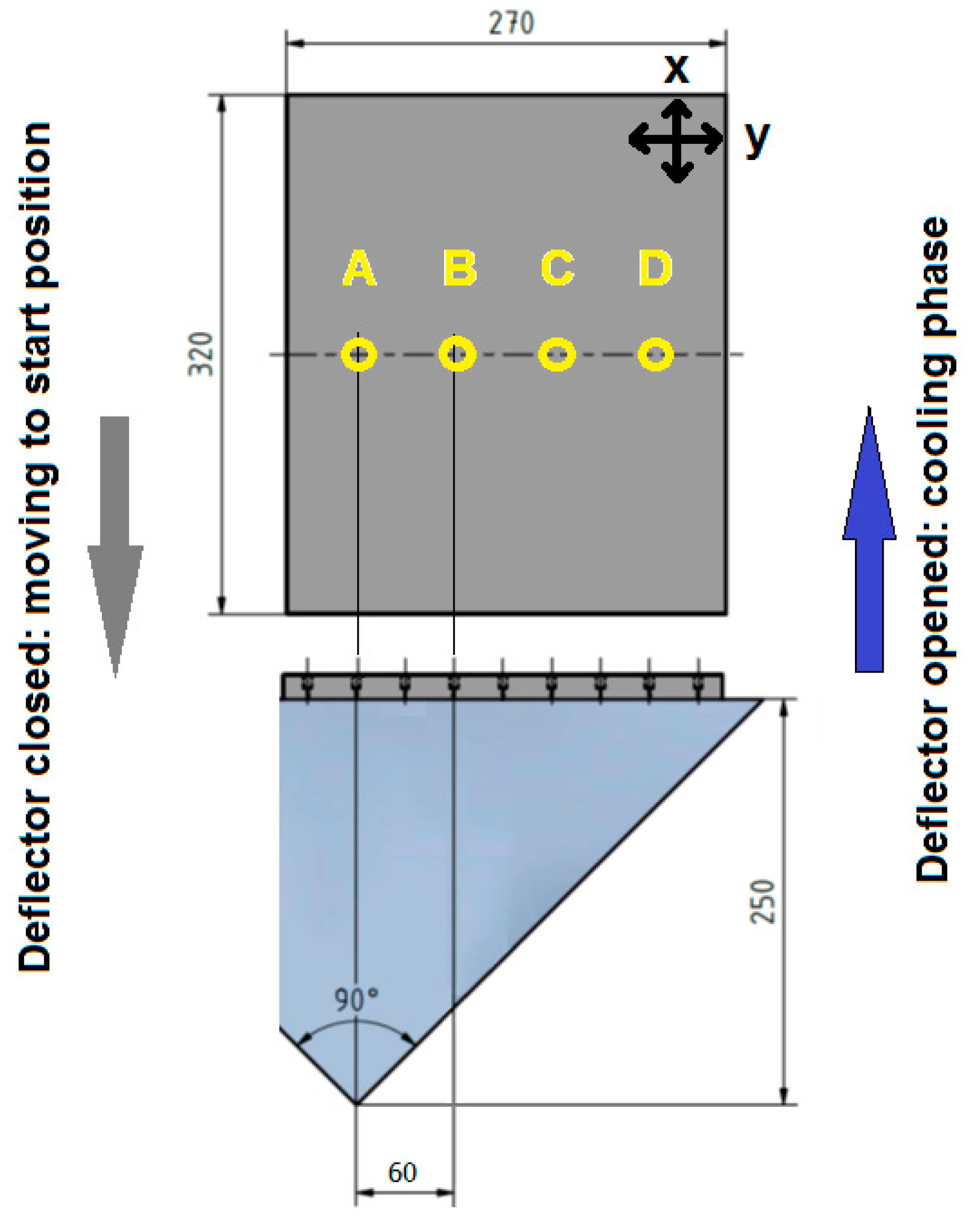
HTC, water impingement density, impact pressure, droplet size and velocity were measured at four points A–D shown in Figure 1. Position A is in the nozzle axis and each other point is at a distance of 60 mm from the previous one.
2.2. Heat Transfer Coefficient Measurement
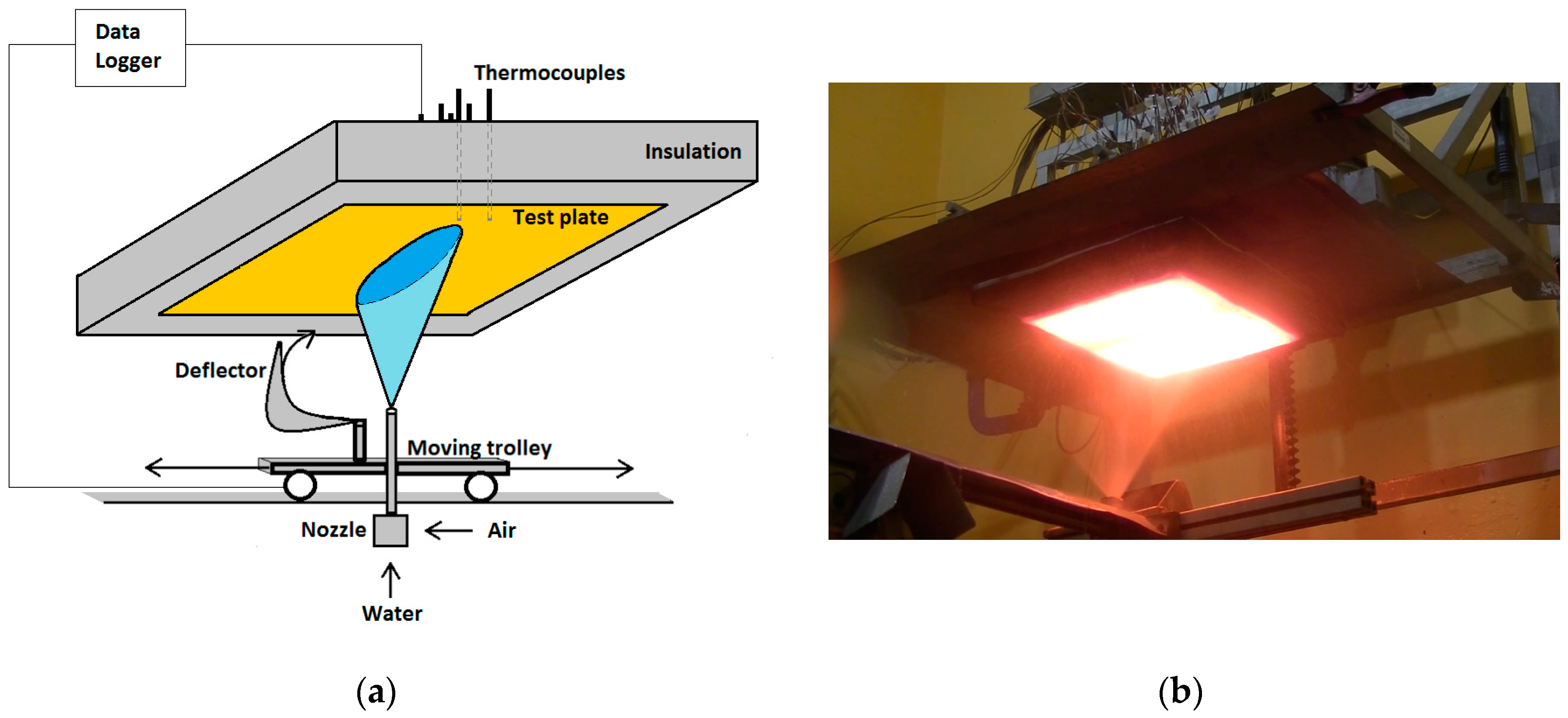
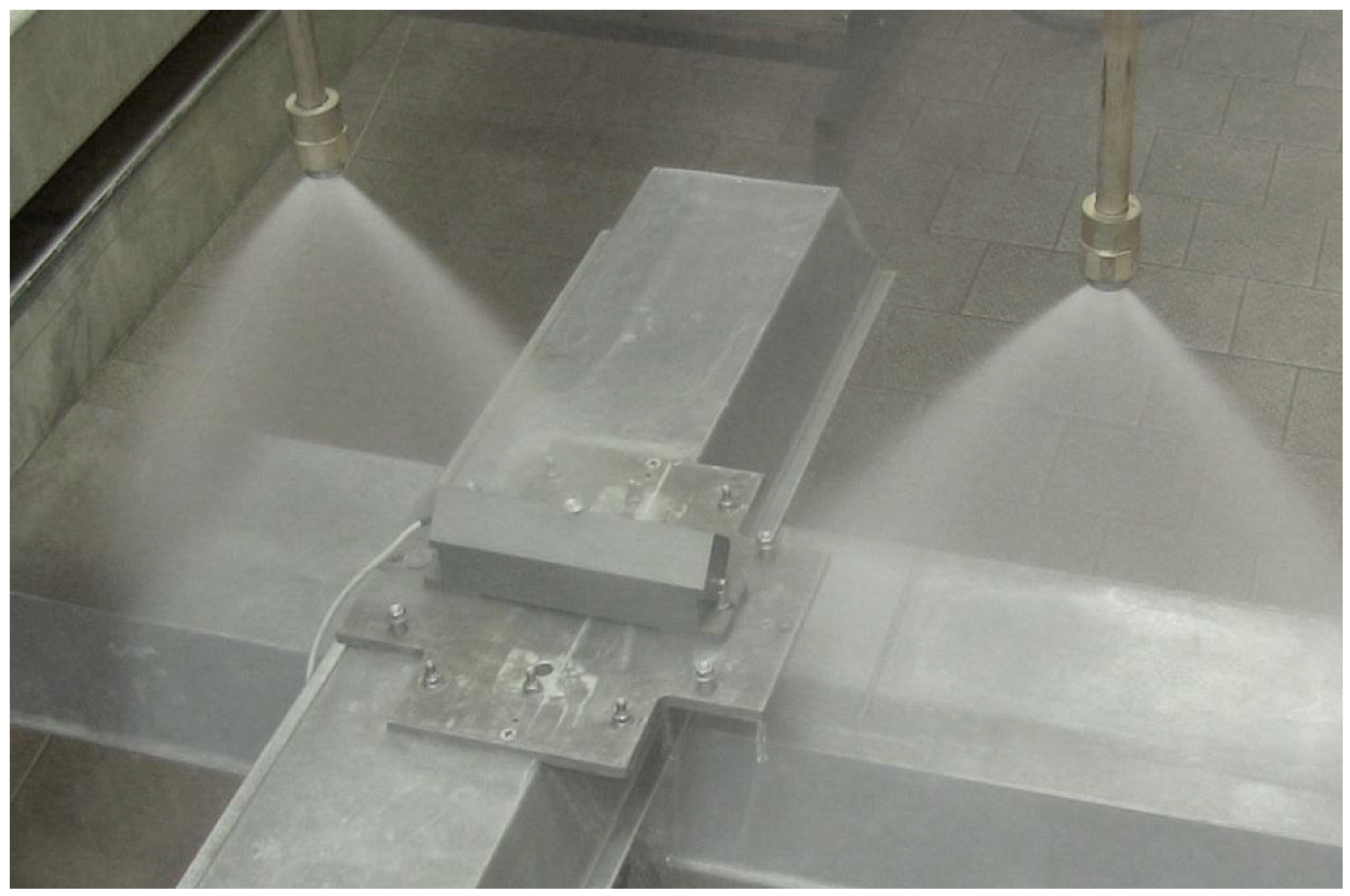
The nozzle being tested was placed under the test plate on a moving trolley (Figure 2). When the nozzle goes in the cooling phase, the deflector is opened and the test plate is cooled by the spray (movement in direction of positive x axis in Figure 1). When the nozzle moves back to the starting position, the deflector is closed and no water can touch the steel surface. The test plate was heated before the experiment to an initial temperature of 1250 °C. This experiment arrangement covers a wide range of surface temperatures. The velocity was set to 1 m min−1 in this study. The test plate is insulated from all sides except the sprayed surface and is made of austenitic steel to protect the surface from oxidation. Austenitic steel is advantageous for inverse heat conduction tasks because of the missing material’s phase changes and subsequent steep changes in thermos-physical properties with temperature. K-type shielded thermocouples are positioned inside the plate with the tip at a distance of 2 mm from the cooled surface. The computer with the data acquisition system monitors the heating process, controls the experiment and records the data from the thermocouples and position sensor.
The experimental data (measured temperatures) were used as input into the inverse heat conduction problem (IHCP) that gives HTC, surface temperature and heat flux in thermocouple positions (A, B, C, D) over time. The numerical model used in evaluation uses the real geometry of the test plate and inner structure of the shielded thermocouples. This approach includes a real thermocouple response time. More about the IHCP used in this study can be found in [23,24].
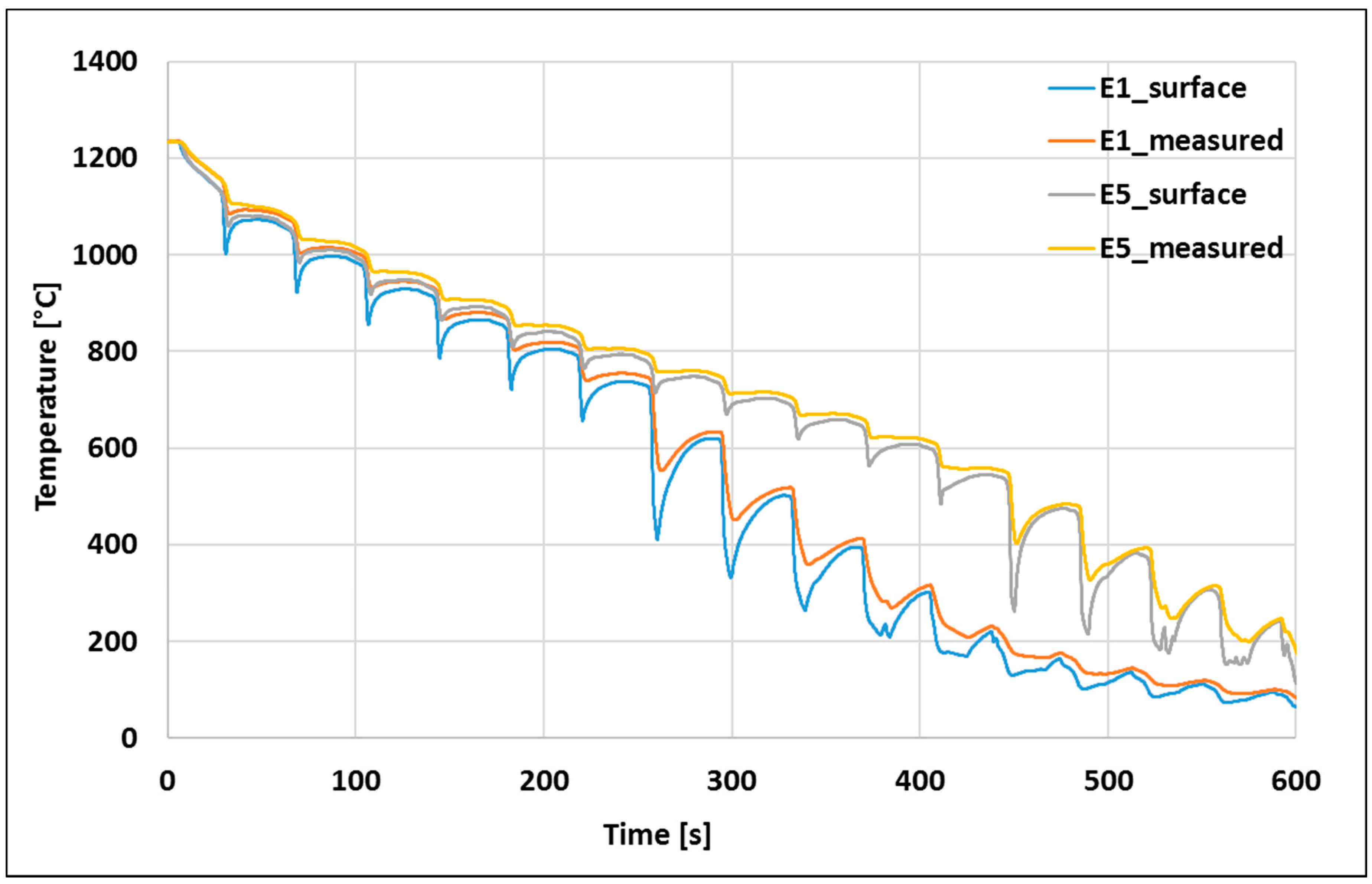
An example of a measured and surface temperature record to the nozzle axis position is shown in Figure 3. The temperature drops on the records indicate the time when the nozzle spray centre of the test plate is where the thermocouples are located. Figure 3 shows data for experiments E1 and E5. Temperature drops are smaller at the beginning of measurement when surface temperature is high and the film boiling regime exists. After several runs under the spray the surface temperature drops under the Leidenfrost temperature and cooling is suddenly much more intensive. It can be seen that there are six paths under the spray for experiment E1 (big water nozzle) above the Leidenfrost temperature. The Leidenfrost temperature can be estimated as 700 °C and below this temperature the temperature drops are much bigger.
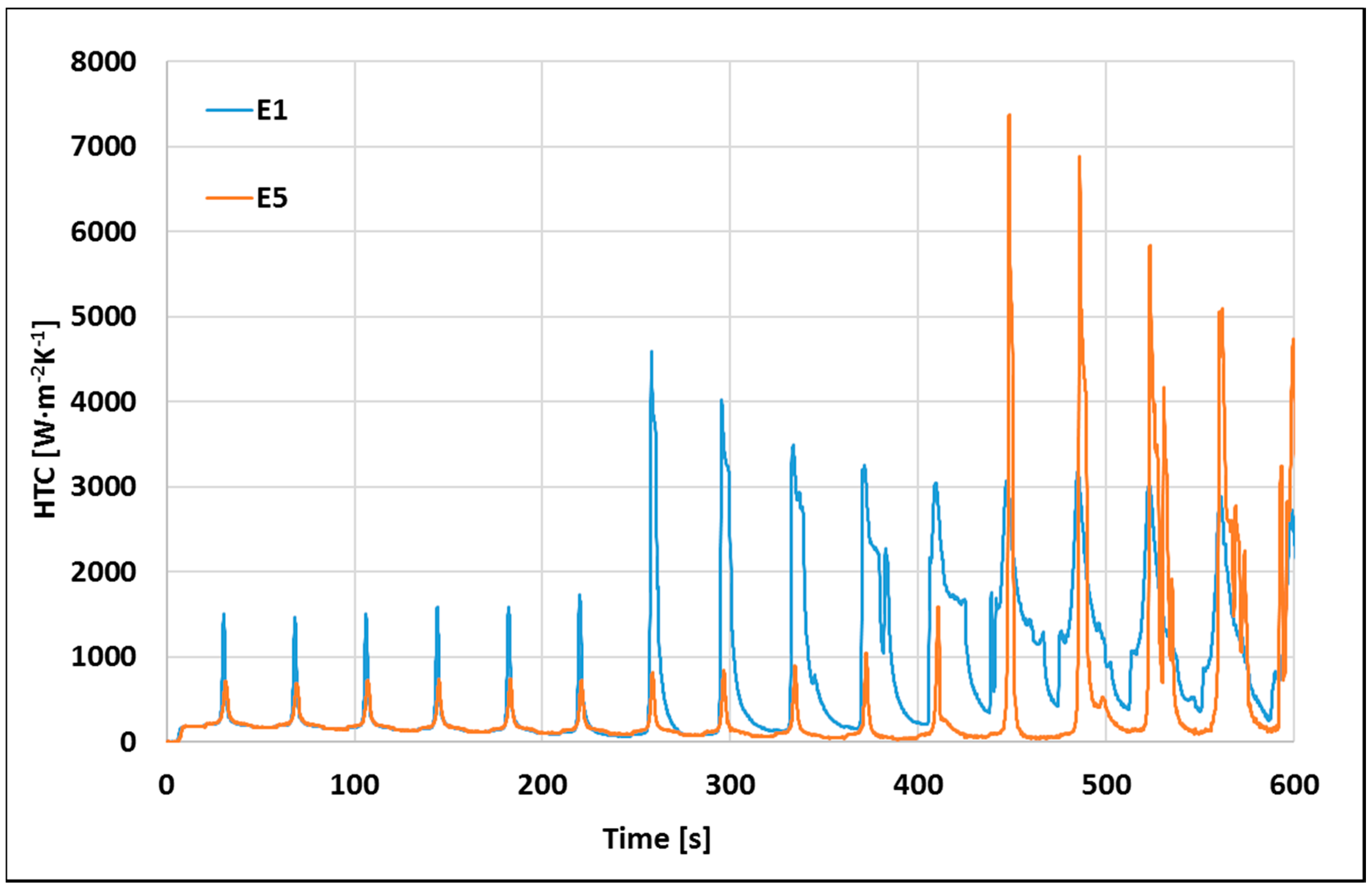
Figure 4 shows HTC history for the measured temperatures shown in Figure 3. The differences between cooling intensity above and below the Leidenfrost temperature are obvious. It should be noted that HTC above the Leidenfrost temperature slowly grows with a decrease in the surface temperature. Another aspect visible in Figure 4 is that HTC below the Leidenfrost temperature cover a wider and wider area on the cooled surface (the HTC impulses become wider with the falling surface temperature).
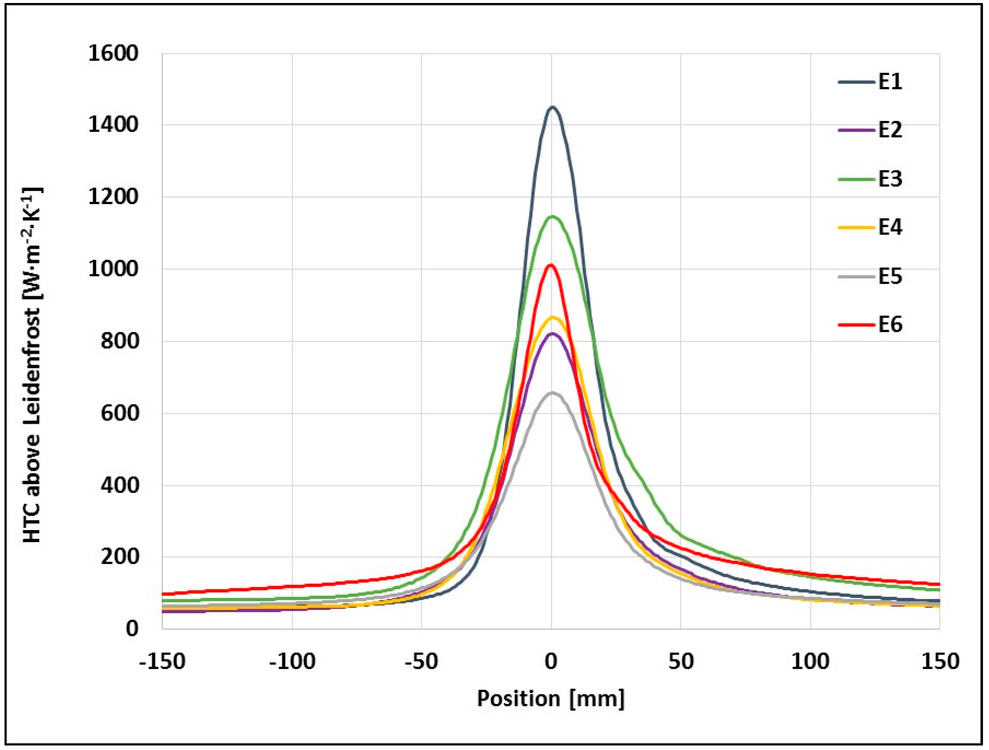
Relative position of the nozzle and test plate was recorded during the experiment. This allows to use distribution of HTC on the cooled surface for evaluation. The averaged HTC distribution for all experiments is shown in Figure 5.
2.3. Water Impingement Density Measurement
The real water flow along the nozzle axis in the y direction was measured by use of a patternator with 10 mm wide slots. The chamber was placed at a distance equal to the experimental spray height of 250 mm. The water impingement density along the nozzle axis was determined in L·m−2s−1.
2.4. Impact Pressure Measurement
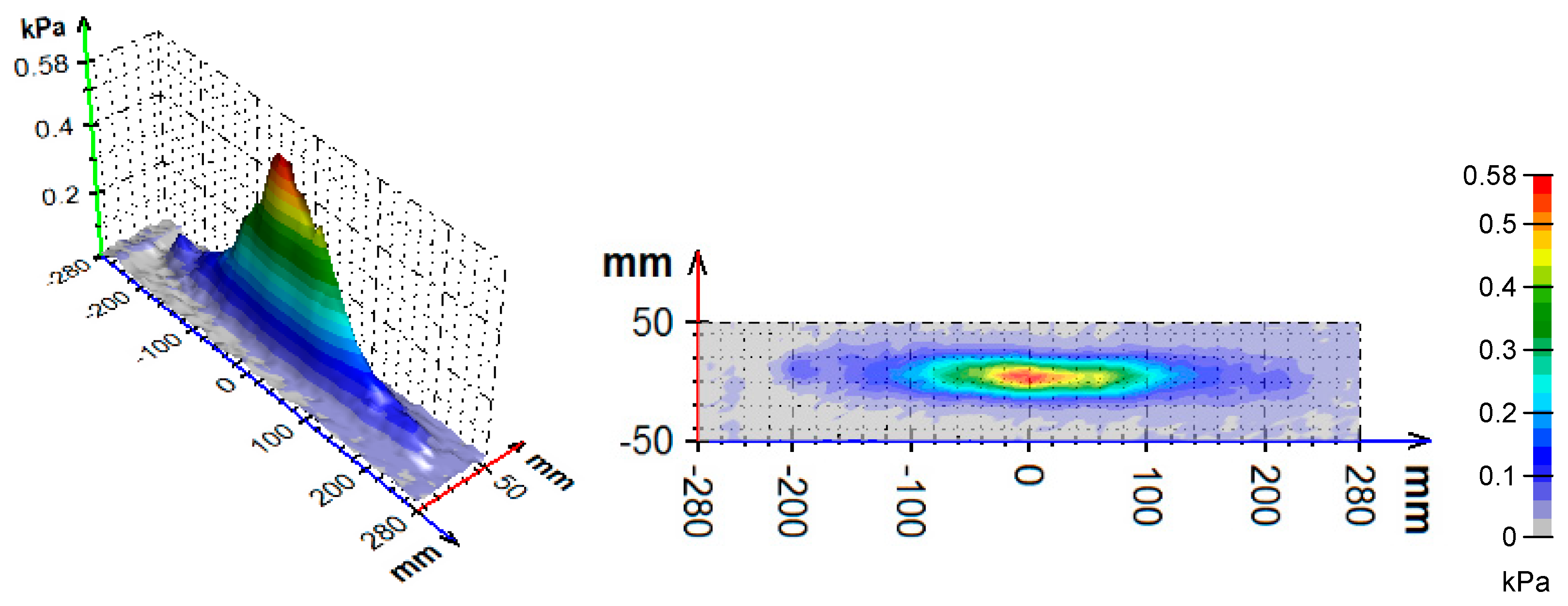
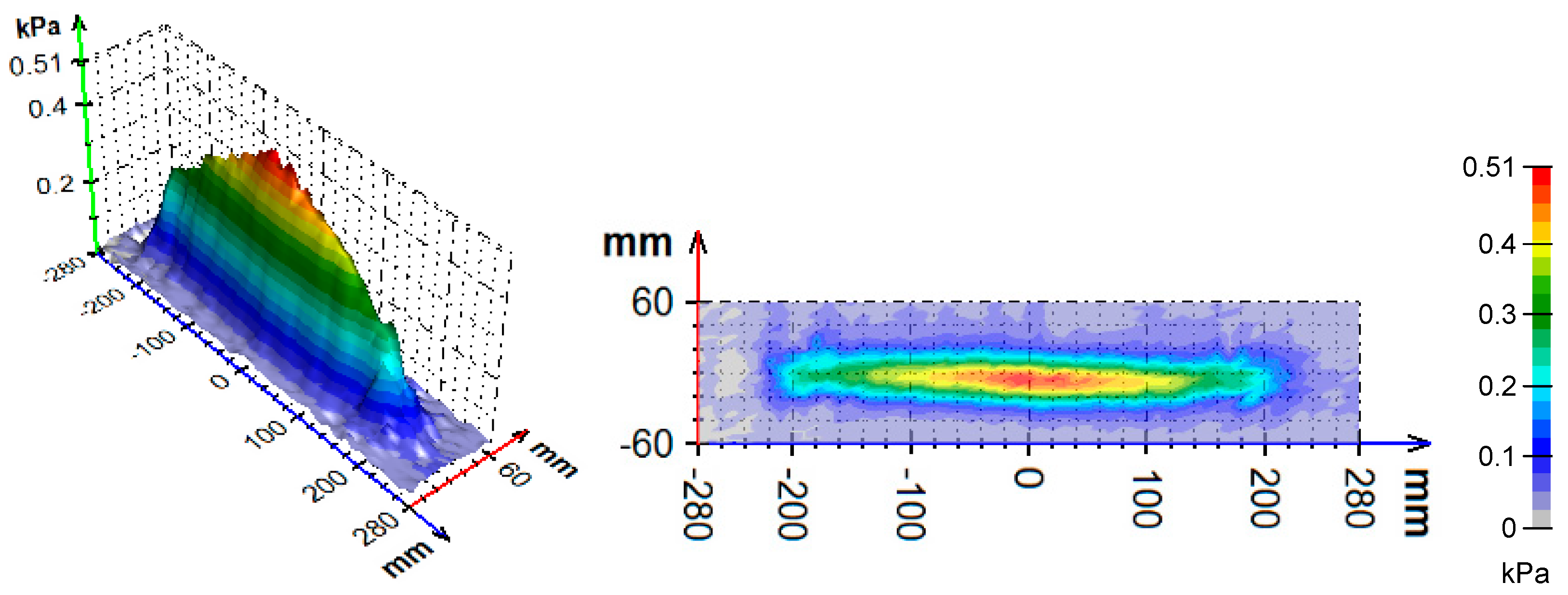
Impact pressure distribution was measured to investigate the impact forces caused by the spray on flat surfaces. For a given nozzle configuration, the pressure sensor moves under the spraying nozzle (Figure 6) and data were recorded together with sensor position. The pressure sensor was formed as a round pin diameter of 10 mm and force measurement was used. Precision of the force sensor is 0.5% of sensor range (0–5 N). The scanning area was 120 mm × 600 mm and measuring was done with a step of 5 mm along the x axis and 10 mm along the y axis. Data were processed by the computer and the result is the field of impact pressures in kPa (Figure 7 and Figure 8). The impact pressures were later averaged for correlation purposes.
2.5. Droplet Size and Velocity
Droplet size and velocity was measured at four locations spaced at 60 mm each other (A–D in Figure 2). Droplets were investigated in free spray at a distance of 250 mm from the nozzle orifice, which is the same as the spray height for HTC measurement. Jet structure and velocity field were measured in cooperation with the Institute of Geonics of the Czech Academy of Sciences by use of optical imaging. The method used is the shadowgraph technique combined with PIV processing algorithms [19] and is shown in Figure 9. Measurement equipment ParticleMaster Shadow manufactured by the company LaVision was used.
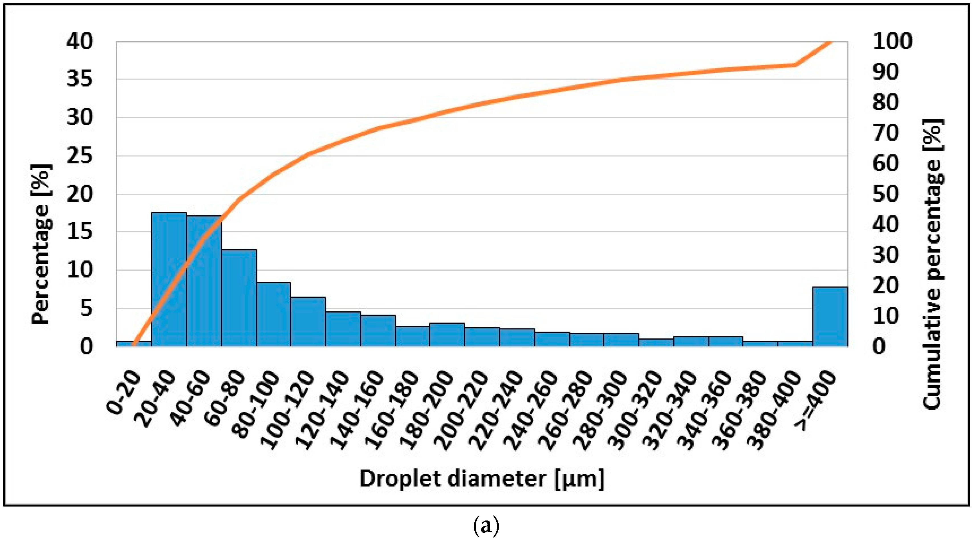
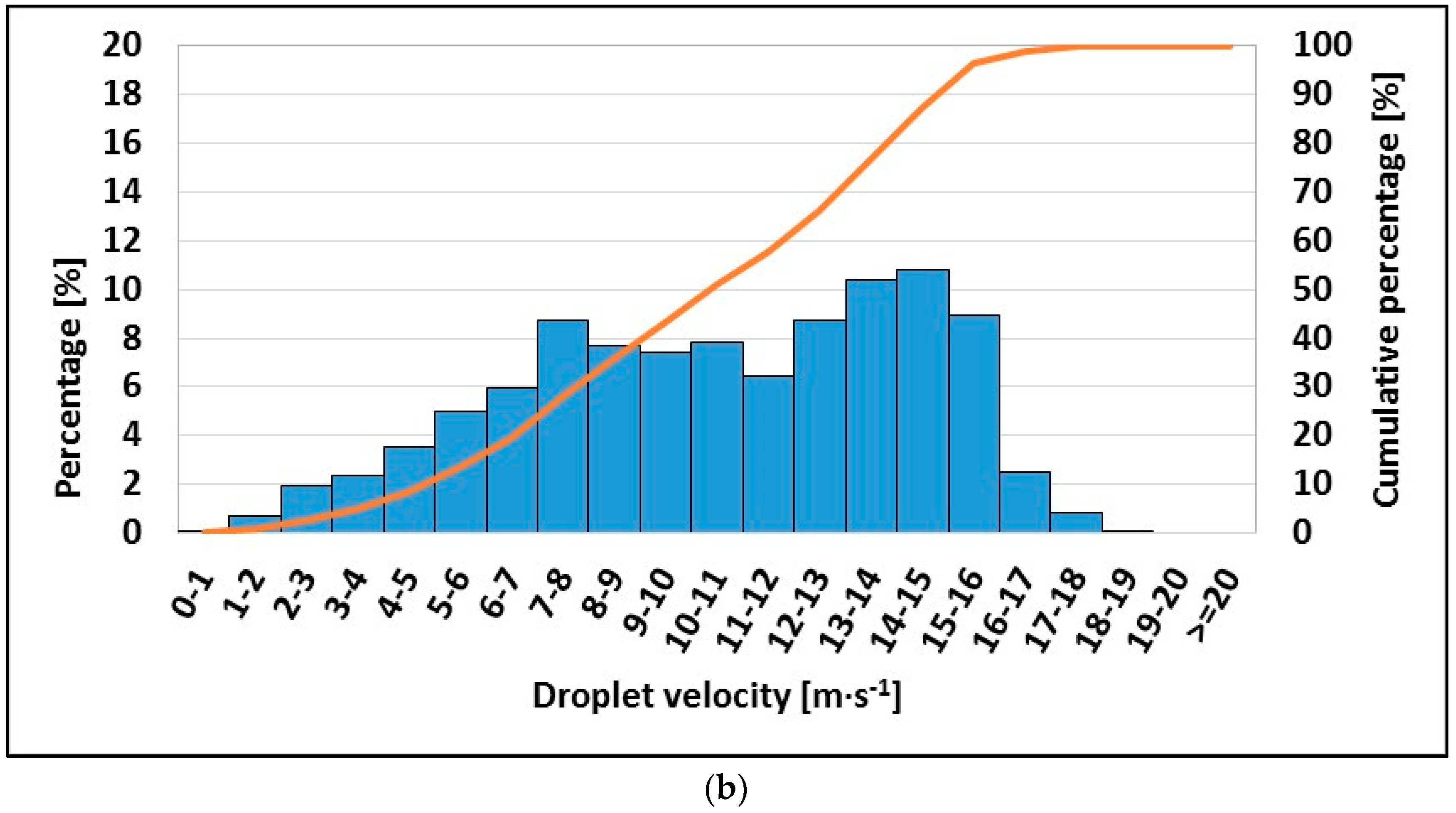
The spray was filmed by a high speed and high resolution CCD camera with double frame mode and was synchronised with the pulsed laser by means of a PTU controller. The double frame camera means that a pair of photos are taken. In our measurement the pairs of photos were taken at a frequency of 15 Hz. We got 400 pairs of photos in total. Mathematical software was able to identify the same droplets in two sequential photos. Each pair of photos had a time shift of 5 ms. After a droplet is identified, the software measures its diameter and calculates velocity. The data of all identified droplets were statistically evaluated and the mean values of the spray were calculated (D10—mean diameter, D32—Sauter mean diameter, VP—absolute mean velocity, VPx mean velocity on x axis, VPy mean velocity on y axis). The graphs shown in Figure 10 and Figure 11 are examples of the data produced from droplet size and velocity measurement.
2.6. Inputs for Correlations
For each experiment setting (six experiments) a complete set of data at four points at different distances from the nozzles axes (A–D, see Figure 1) is available. All of the data are averaged in the “cooling zone”. The cooling zone is 100 mm long (±50 mm from the nozzle axis, see Figure 5). For the heat transfer coefficient only data above the Leidenfrost point are used.
The following parameters are available for correlations:
- Qi [L·m−2s−1] water impingement density,
- v [m·s−1] mean droplet velocity,
- d32 [m] Sauter droplet diameter,
- N [m−2s−1] number of drops per square meter per second,
- E [J] kinetic energy of droplet (for droplet with average size and speed),
- H [kg·m·s−1] droplet momentum,
- Im [Pa] impact pressure
- HTC [W·m−2·K−1] average heat transfer coefficient
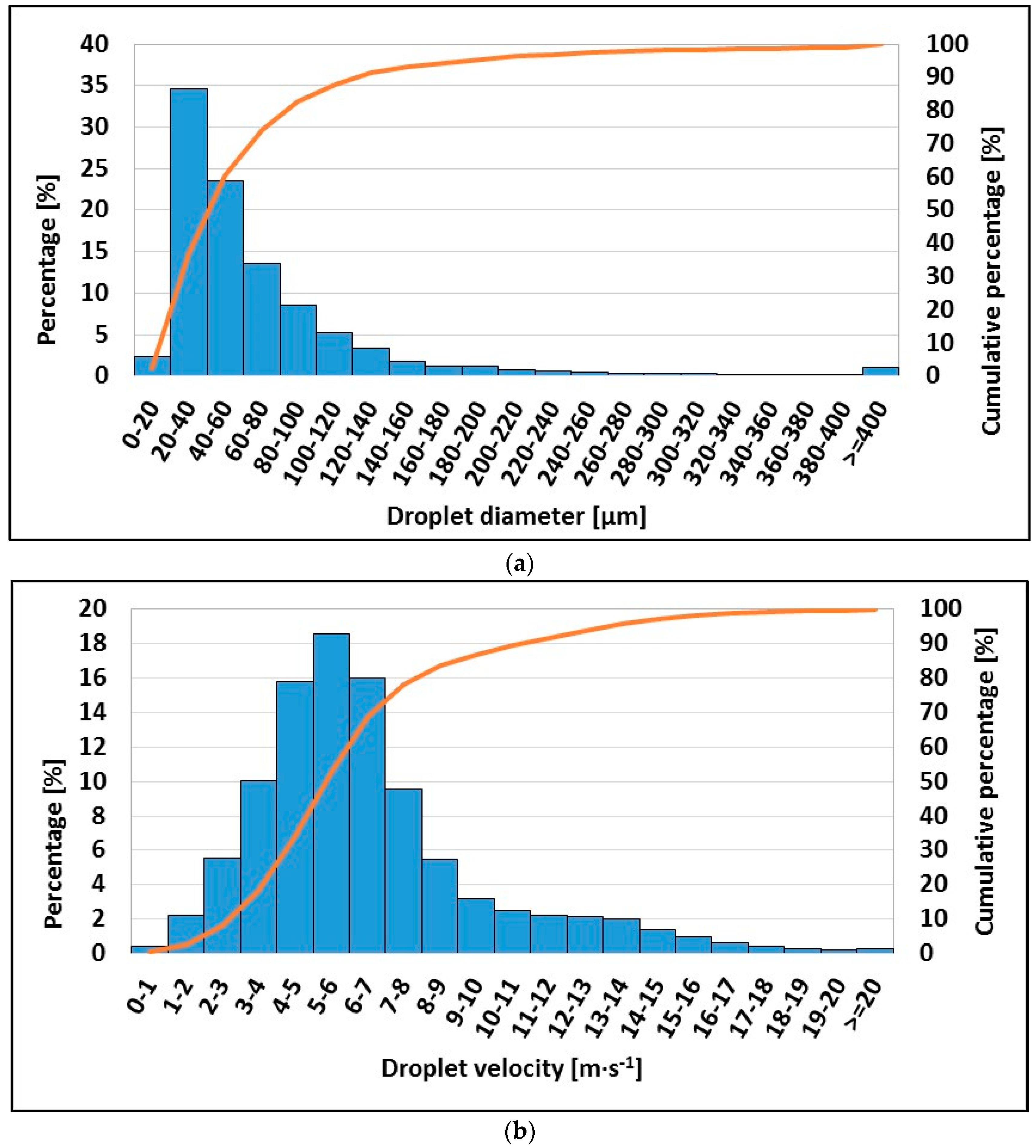
Selected measured data are summarised in Figure 12.
3. Correlations
The following shape of the correlation equation is most frequently used in literature for HTC and is used in this study:
, where are constant and are some of the listed parameters.
Ten combinations of measured spray parameters were selected and constants for correlation functions were computed. A complete list of the correlation functions created is shown in Table 2. The last column “Res2” contains the average square difference between the measured and correlated HTC. , where 24 is the number of HTC values used. for each tested equation is also shown in Figure 13.
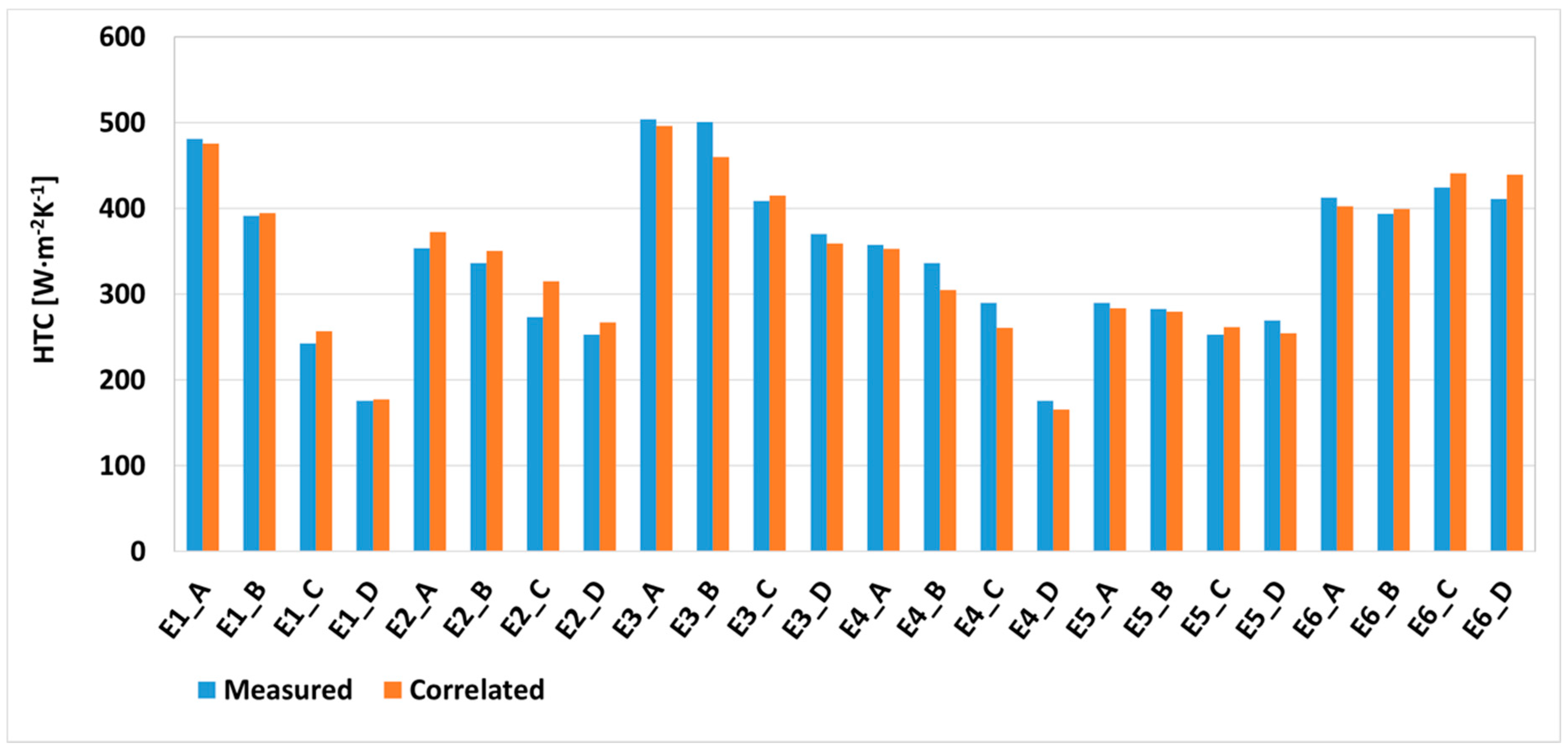
Comparison of measured and correlated HTC above Leidenfrost (Equation (8)) is in Figure 14.
4. Discussion and Conclusions
The best results were obtained when the parameters impact pressure and water impingement density were used together (Equation (8)). A comparison between measured and computed data by Equation (8) is shown in Figure 14.
The worst result is obtained when only water impingement density is used (Equation (10)). This finding should be considered important because correlations based only on water impingement density are the most frequent in the literature. Frequent use of Qi is definitely due to the fact that this parameter is easy to measure.
Equations using droplet size and velocity (Equations (1) and (2)) provide good results. Both equations are equivalent to each other because the number of droplets N (used in Equation (2)) can be expressed by Qi and d32 (used in Equation (1)).
It is interesting to observe the results where instead of v and d32, Re or kinetic energy E is used. Correlations where velocity and droplet diameter are used as separate parameters provide significantly better results in comparison to the equations where these parameters are included in droplet Re or in kinetic energy.
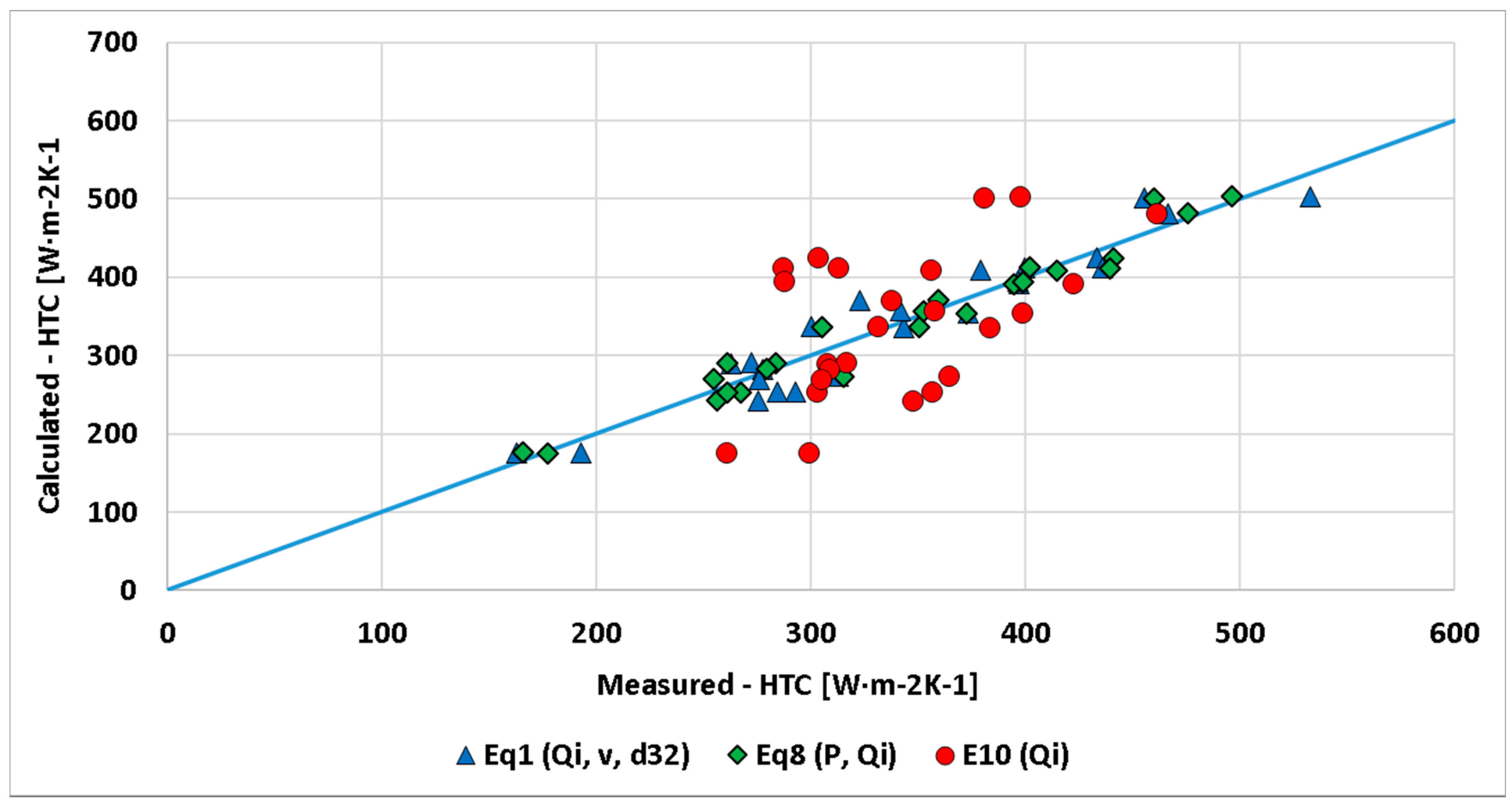
The correlations of measured and calculated HTC based on the Equations (1), (10), (8) are plotted in Figure 15. The difference between the best and worst equations is shown here. Equation (10) is the worst of the tested equations (based on water impingement density only), Equation (1) provides relatively good results (equation based on water impingement density, droplet speed and diameter), Equation (8), which is based on water impingement density and impact pressure, provides the best results.
The presented results can be used for designing a control of cooling units with water spray cooling at high surface temperatres. A typical example is continuous casting and heat treatment.
Author Contributions
Methodology, P.K.; writing—original draft preparation, M.C. and H.B.; writing—review and editing, J.K.; visualization, X.X.; supervision, M.R. All authors have read and agreed to the published version of the manuscript.
Funding
This research was funded by Ministry of Education under the programme INTER EXCELLENCE, within the project LTAUSA19053 and by internal project No. FSI-S-20-6478 of the Brno University of Technology.
Acknowledgments
We thank both nozzle producers, Spraying System and Everloy, who selected and provided the nozzles for this study. The authors gratefully acknowledge the financial support from the Ministry of Education under the programme INTER _ EXCELLENCE, within the project LTAUSA19053 and the Brno University of Technology granted the internal project No. FSI-S-20-6478.
Conflicts of Interest
The authors declare no conflict of interest.
References
- Hernández-Bocanegra, C.A.; Minchaca-Mojica, J.I.; Humberto Castillejos, E.A.; Acosta-González, F.A.; Zhou, X.; Thomas, B.G. Measurement of heat flux in dense air-mist cooling: Part II—The influence of mist characteristics on steady-state heat transfer. Exp. Therm. Fluid Sci. 2013, 44, 161–173. [Google Scholar] [CrossRef]
- Huerta, L.M.E.; Mejía, G.M.E.; Castillejos, E.A.H. Heat Transfer and Observation of Droplet-Surface Interactions During Air-Mist Cooling at CSP Secondary System Temperatures. Metall. Mater. Trans. B 2016, 47, 1409–1426. [Google Scholar] [CrossRef]
- Minchaca, M.J.I.; Castillejos, E.A.H.; Acosta, G.F.A. Size and Velocity Characteristics of Droplets Generated by Thin Steel Slab Continuous Casting Secondary Cooling Air-Mist Nozzles. Metall. Mater. Trans. B 2011, 42, 500–515. [Google Scholar] [CrossRef]
- Xie, J.; Wong, T.N.; Duan, F. Modelling on the dynamics of droplet impingement and bubble boiling in spray cooling. Int. J. Therm. Sci. 2016, 104, 469–479. [Google Scholar] [CrossRef]
- de León, B.M.; Castillejos, E.A.H. Physical and Mathematical Modeling of Thin Steel Slab Continuous Casting Secondary Cooling Zone Air-Mist Impingement. Metall. Mater. Trans. B 2015, 46, 2028–2048. [Google Scholar] [CrossRef]
- Hou, Y.; Tao, Y.; Huai, X.; Zou, Y.; Sun, D. Numerical simulation of multi-nozzle spray cooling heat transfer. Int. J. Therm. Sci. 2018, 125, 81–88. [Google Scholar] [CrossRef]
- Tseng, A.A.; Raudensky, M.; Lee, T.-W. Liquid Sprays for Heat Transfer Enhancements: A Review. Heat Transf. Eng. 2016, 37, 1401–1417. [Google Scholar] [CrossRef]
- Raudensky, M.; Horsky, J. Secondary cooling in continuous casting and Leidenfrost temperature effects. Ironmak. Steelmak. 2005, 32, 159–164. [Google Scholar] [CrossRef]
- Liang, G.; Mudawar, I. Review of spray cooling–Part 2: High temperature boiling regimes and quenching applications. Int. J. Heat Mass Transf. 2017, 115, 1206–1222. [Google Scholar] [CrossRef]
- Liang, G.; Mudawar, I. Review of spray cooling–Part 1: Single-phase and nucleate boiling regimes, and critical heat flux. Int. J. Heat Mass Transf. 2017, 115, 1174–1205. [Google Scholar] [CrossRef]
- Klinzing, W.P.; Rozzi, J.C.; Mudawar, I. Film and transition boiling correlations for quenching of hot surfaces with water sprays. J. Heat Treat. 1992, 9, 91–103. [Google Scholar] [CrossRef]
- Fujimoto, H.; Hatta, N.; Asakawa, H.; Hashimoto, T. Predictable Modelling of Heat Transfer Coefficient between Spraying Water and a Hot Surface above the Leidenfrost Temperature. ISIJ Int. 1997, 37, 492–497. [Google Scholar] [CrossRef] [Green Version]
- Nasr, G.G.; Yule, A.J.; Bendig, L. Background on Sprays and Their Production. In Industrial Sprays and Atomization: Design, Analysis and Applications; Nasr, G.G., Yule, A.J., Bendig, L., Eds.; Springer: London, UK, 2002; pp. 7–33. ISBN 978-1-4471-3816-7. [Google Scholar]
- Ma, H.; Lee, J.; Tang, K.; Liu, R.; Lowry, M.; Silaen, A.; Zhou, C.Q. Modeling of Spray Cooling with a Moving Steel Slab during the Continuous Casting Process. Steel Res. Int. 2019, 90. [Google Scholar] [CrossRef]
- Lefebvre, A.H. Atomization and Sprays; Hemisphere Publishing: New York, NY, USA, 1989. [Google Scholar] [CrossRef]
- Goswami, D.Y. The CRC Handbook of Mechanical Engineering, 2nd ed.; Goswami, D.Y., Ed.; CRC Press: Boca Raton, FL, USA, 2004; ISBN 978-0-8493-0866-6. [Google Scholar]
- Estes, K.A.; Mudawar, I. Correlation of sauter mean diameter and critical heat flux for spray cooling of small surfaces. Int. J. Heat Mass Transf. 1995, 38, 2985–2996. [Google Scholar] [CrossRef]
- Lefebvre, A.H.; Ballal, D.R. Gas. Turbine Combustion, 3rd ed.; CRC Press: Boca Raton, FL, USA, 2010; ISBN 978-1-4200-8605-8. [Google Scholar]
- Zeleňák, M.; Foldyna, J.; Scucka, J.; Hloch, S.; Riha, Z. Visualisation and measurement of high-speed pulsating and continuous water jets. Measurement 2015, 72, 1–8. [Google Scholar] [CrossRef]
- Raudensky, M.; Tseng, A.; Horský, J.; Komínek, J. Recent developments of water and mist spray cooling in continuous casting of steels. Metall. Res. Technol. 2016, 113, 509. [Google Scholar] [CrossRef]
- Cooling When There’s too Much Heat. Available online: http://news.mit.edu/2013/cooling-droplets-1111 (accessed on 3 August 2020).
- Aamir, M.; Qiang, L.; Hong, W.; Xun, Z.; Wang, J.; Sajid, M. Transient heat transfer performance of stainless steel structured surfaces combined with air-water spray evaporative cooling at high temperature scenarios. Appl. Therm. Eng. 2017, 115, 418–434. [Google Scholar] [CrossRef]
- Ondrouskova, J.; Pohanka, M.; Vervaet, B. Heat-flux computation from measured-temperature histories during hot rolling. Mater. Tehnol. 2013, 47, 85–87. [Google Scholar]
- Kominek, J.; Pohanka, M. Estimation of the Number of Forward Time Steps for the Sequential Beck Approach Used for Solving Inverse Heat-Conduction Problems. Mater. Tehnol. 2016, 50, 207–210. [Google Scholar] [CrossRef]
Figure 1.
Scheme of the measurement, all data are available in points A–D. (Dimensions are in mm).

Figure 2.
Scheme of experiment (a), test plate with thermocouples and nozzle with deflector on moving trolley for the heat transfer coefficient (HTC) measurement (b).
Figure 2.
Scheme of experiment (a), test plate with thermocouples and nozzle with deflector on moving trolley for the heat transfer coefficient (HTC) measurement (b).

Figure 3.
Temperatures measured at a depth of 2 mm and computed surface temperatures, data for experiments E1 and E5 in position of nozzle axis.
Figure 3.
Temperatures measured at a depth of 2 mm and computed surface temperatures, data for experiments E1 and E5 in position of nozzle axis.

Figure 4.
HTC vs. time on the nozzle axis (position A) for experiment E1 and E5.

Figure 5.
HTC averaged from runs above the Leidenfrost temperature for thermocouple “A” (y = 0 mm).

Figure 6.
Impact pressure measurement, pin diameter of 10 mm on moving x–y table.

Figure 7.
Impact pressure distribution for experiment E1.

Figure 8.
Impact pressure distribution for experiment E3.

Figure 9.
Schematic of experimental apparatus.

Figure 10.
Droplet diameter (a) and droplet velocity (b) scatter plotted for E1 in position A.


Figure 11.
Droplet diameter (a) and droplet velocity (b) scatter plotted for E5 nozzle in position A.
Figure 11.
Droplet diameter (a) and droplet velocity (b) scatter plotted for E5 nozzle in position A.

Figure 12.
Summary of averaged measured data: HTC, water impingement density, impact pressure, Sauter mean diameter of the droplet d32, droplet mean velocity vp for all experiments.
Figure 12.
Summary of averaged measured data: HTC, water impingement density, impact pressure, Sauter mean diameter of the droplet d32, droplet mean velocity vp for all experiments.

Figure 13.
Comparison of Equations (1)–(10) based on Res2. The parameters that were used are written under each column.
Figure 13.
Comparison of Equations (1)–(10) based on Res2. The parameters that were used are written under each column.

Figure 14.
HTC above Leidenfrost measured and correlated (Equation (8): ).

Figure 15.
Correlation between measured HTC and calculated HTC for three selected equations.


Table 1.
List of experiments.
| Experiment | Water Flowrate [L/min] | Air Pressure [Bar] | Nozzle Type |
|---|---|---|---|
| E1 | 11.0 | NA | Large water |
| E2 | 11.0 | 1.5 | Large mist low |
| E3 | 11.0 | 3.0 | Large mist high |
| E4 | 6.0 | NA | Small water |
| E5 | 6.0 | 0.5 | Small mist low |
| E6 | 6.0 | 1.5 | Small mist high |
Table 2.
List of tested correlations.
| ID | Formula | Res2 |
|---|---|---|
| Equation (1) | 664 | |
| Equation (2) | 664 | |
| Equation (3) | 5999 | |
| Equation (4) | 5536 | |
| Equation (5) | 1402 | |
| Equation (6) | 2957 | |
| Equation (7) | 672 | |
| Equation (8) | 340 | |
| Equation (9) | 894 | |
| Equation (10) | 6034 |
© 2020 by the authors. Licensee MDPI, Basel, Switzerland. This article is an open access article distributed under the terms and conditions of the Creative Commons Attribution (CC BY) license (http://creativecommons.org/licenses/by/4.0/).
Share and Cite
MDPI and ACS Style
Chabicovsky, M.; Kotrbacek, P.; Bellerova, H.; Kominek, J.; Raudensky, M. Spray Cooling Heat Transfer above Leidenfrost Temperature. Metals 2020, 10, 1270. https://doi.org/10.3390/met10091270
AMA Style
Chabicovsky M, Kotrbacek P, Bellerova H, Kominek J, Raudensky M. Spray Cooling Heat Transfer above Leidenfrost Temperature. Metals. 2020; 10(9):1270. https://doi.org/10.3390/met10091270
Chicago/Turabian StyleChabicovsky, Martin, Petr Kotrbacek, Hana Bellerova, Jan Kominek, and Miroslav Raudensky. 2020. "Spray Cooling Heat Transfer above Leidenfrost Temperature" Metals 10, no. 9: 1270. https://doi.org/10.3390/met10091270
Note that from the first issue of 2016, this journal uses article numbers instead of page numbers. See further details here.