Characterization of the Density and Spatial Distribution of Dispersoids in Al-Mg-Si Alloys


Department of Materials Science and Engineering, Norwegian University of Science and Technology, NO-7491 Trondheim, Norway
*
Author to whom correspondence should be addressed.
Metals 2019, 9(1), 26; https://doi.org/10.3390/met9010026
Submission received: 30 November 2018
/
Revised: 14 December 2018
/
Accepted: 21 December 2018
/
Published: 28 December 2018
Abstract
:Al-Mg-Si alloys often contain small additions of, for example, Mn or Cr, to form dispersoids, which may act as nucleation sites for Mg2Si particles after homogenization. The purpose of adding Mn and Cr is to ensure a high density of uniformly distributed small β’-particles, which can be dissolved during further processing prior to the final age hardening step. However, their density and spatial distribution are critically dependent on the homogenization procedure. It is therefore important to have a robust and reliable method for assessing their spatial distribution. In the present work, an existing methodology for assessing spatial uniformity, the Global Shannon Entropy (GSE), was implemented and evaluated for different dispersoid structures characterized by scanning electron microscopy. This metric is highly dependent on the parameters used, but by careful selection of adequate parameters, it can be effective in detecting non-uniformity. An important weakness with the GSE was identified, and a modification to improve on the ability to differentiate degrees of non-uniformity is suggested. To evaluate the proposed methodology, the effect of heating rate on dispersoid precipitation behaviour during homogenisation of four Al-Mg-Si alloys with different Mn/Cr-content was investigated. In general, the dispersoid density increased with decreasing heating rates as longer times in the furnace resulted in particle coarsening. Slower heating rates were found to promote a more uniform dispersoid structure for most alloys investigated in this study. The metric with the new term demonstrated promising results, and improved the ability to differentiate degrees of spatial uniformity.
1. Introduction
Al-Mg-Si series alloys are the most common aluminium extrusion alloys and are attractive for applications in a range of sectors, e.g., construction, automotive, and recently also in consumer electronics, due to their generally good combination of strength, ductility, and corrosion resistance. However, their extrudability and end properties depend critically on the alloy chemistry as well as prior processing conditions. Coarse β-AlFeSi or Mg2Si-particles typically have a detrimental effect on extrudability, while small dispersoid particles may affect recrystallization, grain growth, and precipitation of Mg and Si. The strengthening potential in the final age hardening step depends strongly on the amount of Mg and Si in solid solution after extrusion. The manner in which the different second-phase particles are spatially distributed decide whether the final product exhibits uniform properties, and the number density and sizes determines the extent of the effect.
Al-Mg-Si alloys often have alloy additions, like Mn, Cr, and Zr, which form dispersoids. With a relatively high level of Mn, the dispersoids act as recrystallization inhibitors, and their number density and spatial distribution will have a large influence on the final grain sizes and their uniformity. Even with small additions of Mn, the dispersoids may be important, e.g., to increase the kinetics of β-AlFeSi to α-Al(FeMn)Si primary particle transformation [1]. Dispersoids may also act as potent nucleation sites for β’-Mg2Si, which leads to a higher quench sensitivity as the number density of dispersoids increases. Generally, this is regarded as a negative effect, as it may reduce the ageing potential after extrusion. However, if the dispersoids can be used to control the precipitation of Mg and Si during cooling from homogenisation, the extrudability may be significantly improved.
During homogenisation, coarse Mg2Si particles present after casting or precipitated during heating, dissolve as the heat treatment proceeds. However, they may re-precipitate during cooling, and reduce the extrudability of the billets [2,3]. With a sufficiently slow cooling rate, Mg and Si precipitate as coarse β-Mg2Si particles on grain boundaries in the temperature range of ~525–425 °C depending on the alloy composition [4]. If these particles are sufficiently large (>1 μm), they have been found to have a negative impact on the extrusion speed by causing local melting in the surface area of the billets, as temperature increases during the extrusion process [5,6]. Moreover, if the Mg2Si-particles are large, they will not dissolve completely during extrusion and, hence, the final ageing potential is reduced.
If the size and spatial distribution of dispersoids are carefully controlled as well as the cooling rate, the dispersoids may act as nucleation sites for smaller β’-Mg2Si particles precipitating during cooling after homogenization (formed in the temperature range of 425–250 °C, if there is Mg and Si left in solid solution [4]). These finer β’-precipitates will dissolve as the temperature increases during extrusion, allowing for higher extrusion speeds, while lowering the extrusion pressure as Mg and Si are bound to non-hardening particles, leaving Mg and Si available for age hardening after extrusion. However, if the dispersoids are to act as nucleation agents to control the sizes of the β’-phase, it is critical to control the dispersoid density and spatial distribution. A low number density of dispersoids should result in larger β’-particles, while a higher density should yield smaller β’. As Mg and Si are fairly homogeneously distributed during homogenisation, a uniform spatial distribution of dispersoids is also essential to ensure homogeneous precipitation of β’ during cooling. If an area is depleted of dispersoids, precipitation of coarse β-Mg2Si on grain boundaries may occur in that area, and as mentioned above, such coarse particles are detrimental to the extrudability of the billet [6,7].
In view of the apparent importance of the dispersoid density and spatial distribution on the precipitation behaviour of Mg2Si-particles after homogenisation, and thus their influence on the subsequent processing and final ageing potential, it is important to be able to characterize the precipitation behaviour of dispersoids, both in terms of density and spatial distribution. Even challenging with regard to sample preparation and image processing, quantifying the dispersoid density is mainly straightforward. However, a robust and reliable methodology to assess the spatial precipitation is not equally obvious. Although various approaches exist—some of which will be reviewed in the next section—their application and the assessment of their suitability and performance are limited.
An important objective of the present study is therefore to develop a reliable procedure for the characterization of the density and spatial distribution of dispersoids in aluminium alloys. Scanning electron microscopy (SEM) was used to characterize the dispersoid structures in different aluminium alloys and conditions, while an existing methodology for assessing spatial uniformity, the Global Shannon Entropy (GSE), was implemented and evaluated to assess their spatial distribution. To test and evaluate the proposed methodology, the dispersoid precipitation behaviour during different homogenisation procedures of four Al-Mg-Si alloys with different Mn/Cr-content was investigated. Based on the precipitation model of Lodgaard and Ryum [8], it was assumed that staying for different times at the temperature ranges associated with the different intermediate phases precipitated during heating to homogenisation would affect the density and spatial distribution of dispersoids after homogenisation. Therefore, three different heating rates to the homogenisation holding temperature were chosen to form the basis of this study.
The outline of the paper is as follows. After a brief introduction to different methods for assessing spatial uniformity, a more detailed presentation of the Global Shannon Entropy (GSE) methodology is given. Its ability to characterize non-uniformity is then analysed and discussed by means of a generic study of computer generated point patterns with different degrees of non-uniformity, and a slightly modified metric is suggested. The general methodology for the characterization of the dispersoid structures, in terms of number density, area fraction for the four alloys, and the effect of the heating rate on dispersoid precipitation behaviour during homogenization are then evaluated and discussed, with special attention to the efficiency of the modified GSE metric.
2. Methodology
2.1. Existing Methods for Assessing Spatial Uniformity
Robust and reliable quantitative methods for assessing the spatial distribution of, e.g., particles and precipitates in the aluminium matrix, have mainly been missing, and today, the evaluation is usually done manually and qualitatively by human operators. This may cause the results to vary greatly with the operator on duty. Such evaluations of dispersoid distributions may, for example, be done by measuring the width of the dispersoid-free zones (DFZs) [9], or measuring the change in density from the grain boundary towards the center of the grain [10]. These methods are time consuming and may be inaccurate and inadequate. Efforts have been made both by Marthinsen et al. [11] and Lodgaard and Ryum [12] to implement approaches for the quantification of the spatial distribution of primary particles and dispersoids in aluminium, respectively. The former employed the well-known Johnson-Mehl-Avrami-Kolmogorov (JMAK) theory [13,14,15], in a tessellation procedure, where the particles were converted to dimensionless points, and used as nucleation sites for “site saturation recrystallization”. As the “grains” are allowed to grow and impinge, so-called “Voronoi patterns” are created. The transformation kinetics of the growth process is given by
where Xv represents the fraction recrystallized (or amount of “growth”), k is a constant, and n is the so-called JMAK exponent. In the situation of site saturation (all nuclei start growing at t = 0) of a random distribution of nucleation sites in two dimensions, the JMAK exponent, n, is equal to 2. Thus, the spatial distribution may be evaluated by n’s deviation from 2. By using this method, one would get an idea of both the spatial distribution of primary particles, and the final grain size in the case of recrystallization by particle-stimulated nucleation (PSN). Lodgaard and Ryum [12] developed a method where a threshold was used to separate dispersoid-containing areas from areas empty of dispersoids. The latter area, Ae, was used as a measure of the spatial distribution of dispersoids. A large Ae represents a large area without dispersoids, and consequently a poor spatial distribution. However, this method is more convenient for lower magnifications, and clearly defined DFZs. On the other hand, if the magnification is low, the smallest dispersoids may not be detected, and the results may become inaccurate. Moreover, a low dispersoid density will make it challenging to identify the DFZ, and where Ae begins and ends.
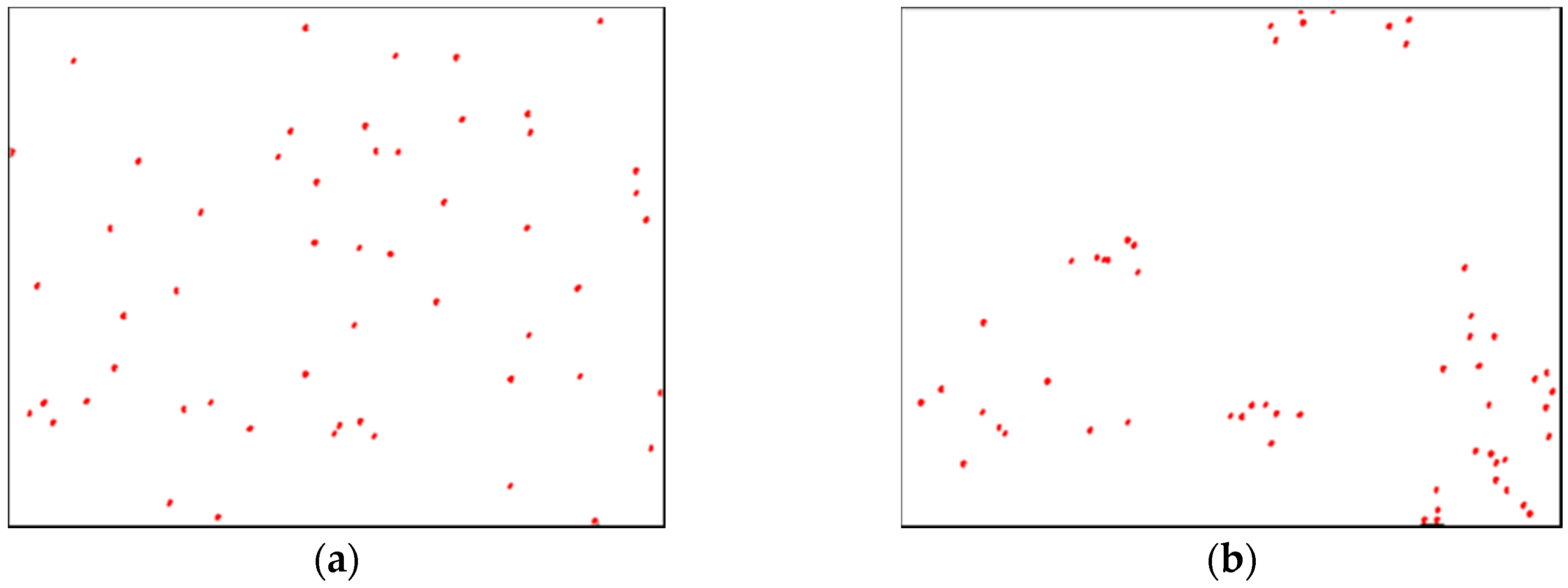
However, recent years’ interest in metal matrix nanocomposites (MMNCs) has resulted in an intensified effort in implementing mathematical models for the assessment of spatial particle distributions. In these materials, nano-sized ceramic particles are embedded into a metal matrix and the uniformity of their distribution is critical to their performance in terms of mechanical properties. Zhou et al. [16] and Kam et al. [17] have given thorough reviews of such metrics, and compared their effectiveness in various tests. In these metrics, particles are treated as dimensionless points, and the resulting patterns are referred to as spatial point patterns. To provide a reference, patterns of complete spatial randomness (CSR) are created, and a specific pattern of interest is tested and compared to the CSR pattern to assess their uniformity (or more precisely their deviation from complete spatial randomness). The CSR patterns are thus regarded as having optimal uniformity. Examples of a CSR pattern and a non-uniform pattern are found in Figure 1.
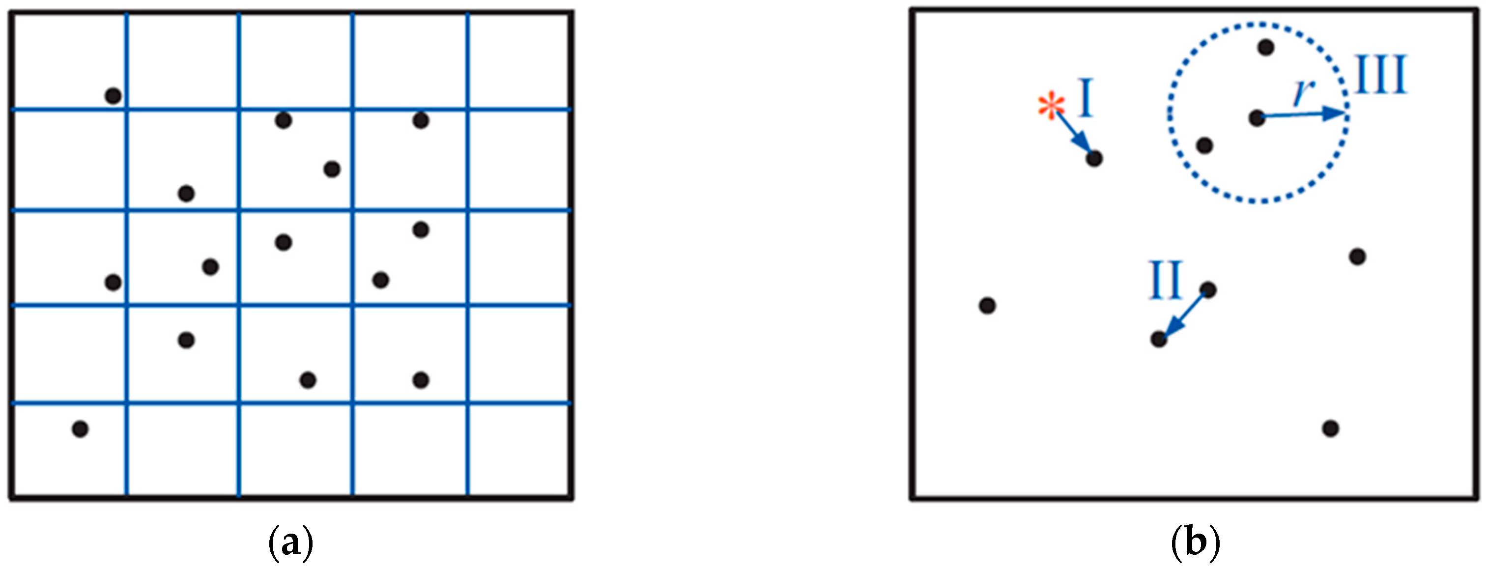
There are two main ways of quantifying the uniformity of spatial point patterns, namely with quadrat-based metrics and distance-based metrics. Distance-based metrics are based on the distances between each point. Other methods exist, but will not be considered here (for more information, see [16,17,18]). In the quadrat-based metrics, the image is separated into a grid of a certain number of quadrats (q), as illustrated in Figure 2a. Each point is then allocated to a grid, and the manner in which the points are distributed over the grids is used as the basis for the calculation of the different metrics. Quadrat-based methods are simple and convenient, but one of their weaknesses is that they do not provide spatial information about the points inside each quadrat. Distance-based metrics, illustrated in Figure 2b, provide more spatial information, but also have their drawbacks. These metrics are based on the distances between each point. However, it was pointed out by Cressie [18] that it is arbitrary if the nearest neighbour, second-nearest, third-nearest etc. are chosen, and this may largely influence your results. Moreover, a problem arises when a point is located closer to the frame of the image than any other point. This is known as the “edge-effect”, and several methods have been developed to account for this (e.g., [19]).
In general, the quadrat-based metrics, Index of Dispersion (ID) and Global Shannon Entropy (GSE), are found to be both more effective and convenient than the distance-based metrics. They are therefore explored further in this study to assess the spatial distribution of dispersoids in aluminium alloys. According to Kam et al. [17], the GSE metric is found best at being able to detect non-uniformity in all the variations of patterns the metrics were tested on. In their studies, the probability of the metric to detect non-uniformity in patterns of different levels of non-uniformity was referred to as the detection power. The detection power is thereby the fraction of patterns not accepted as uniform. Critical values for the metrics with an unknown null distribution were found based on the generation of 10,000 CSR patterns, and using a 95% significance level. In addition to testing the detection power, Zhou et al. [16] also made an effort to test the ability of the metric to differentiate the degree of non-uniformity of different patterns. In their study, all the metrics were found inadequate to differentiate reliably the degree of non-uniformity between different patterns, including the GSE. However, in our opinion, this conclusion is not relevant to the approach used in the present work. This point will be further discussed later in this section. Moreover, a new approach to quantify non-uniformity, which may improve differentiability, will be suggested. Due to the generally good results of the GSE metric, this method was chosen as the basis for the modified metric.
2.2. Global Shannon Entropy (GSE)
The GSE is an entropic measure, where the probability of a point falling into a certain quadrat, pi, is calculated for each quadrat in an image grid. The GSE is then calculated through:
where xi is the number of points found in quadrat i. Under perfect uniformity, pi will be equal for all quadrats, namely pi = 1/q, and GSE = 1. This ideal situation, however, may only occur under conditions of regularity, which rarely occur in nature. CSR patterns, which better reflect the ideal for spatial distributions, such as those for dispersoids, will return a GSE lower than 1. How much lower is dependent on the parameters in use. Moreover, as non-uniformity increases, the GSE decreases until all points are found in one quadrat, and GSE = 0.
The aim of the following section is to evaluate whether the GSE may be useful in quantifying the spatial uniformity of dispersoids in aluminium alloys. In this regard, differentiating the degree of non-uniformity is the main concern. A new simple approach for improving the GSE metric is presented and evaluated.
2.3. Generation of Spatial Point Patterns
The GSE was calculated from a sample population of 100 spatial point patterns to be comparable with the results from backscatter scanning electron microscopy (SEM) (Zeiss Ultra 55 LE, Carl Zeiss AG, Oberkochen, Germany). The resolution of the generated images was also set equal to the SEM images, with an area of, A = 23–33 µm. Each “image” was given a random number of points, based on the density chosen, n (average number of points per image). The CSR patterns were generated by assigning random x- and y-coordinates to each point in a pattern, until the amount of points in each pattern, xi, was fulfilled. To test the efficiency of the GSE metric in detecting non-uniformity, cluster patterns were chosen, as they have been found to pose the biggest challenge for the metrics [16,17]. The cluster patterns were generated in the following way.
- A point is given random x- and y-coordinates.
- Based on the location of the first point, new points are distributed at distances around this location, based on a normal distribution. If a point lands outside the image boundaries, the generation process will continue regardless, and the cluster will contain one less point. The amount of points per cluster will be referred to as nc.
- The generation process is continued until the desired number of points in the image, xi, is fulfilled.
- The intensity of clustering is changed by varying the number of points in each cluster, nc, and the standard deviation in the normal distribution, σ. The standard deviation is set to be a factor multiplied with the maximum dispersoid radius (150 nm), e.g., σ = 5rmax.
2.4. Effect of Point Intensity and Number of Quadrats (q) on the GSE Metric
Due to the nature of the quadrat-based metrics, they will necessarily be dependent on the intensity of points in the patterns. The more points, the higher the metric will score for a given spatial distribution, until the value saturates at a certain intensity. Non-uniform patterns must therefore always be tested against CSR patterns with the same average density, n, as a point of reference. This reduces the “smoothing effect”, making it easier to compare the spatial distribution of samples with different densities. In the current study, all patterns were normalized in the following way:
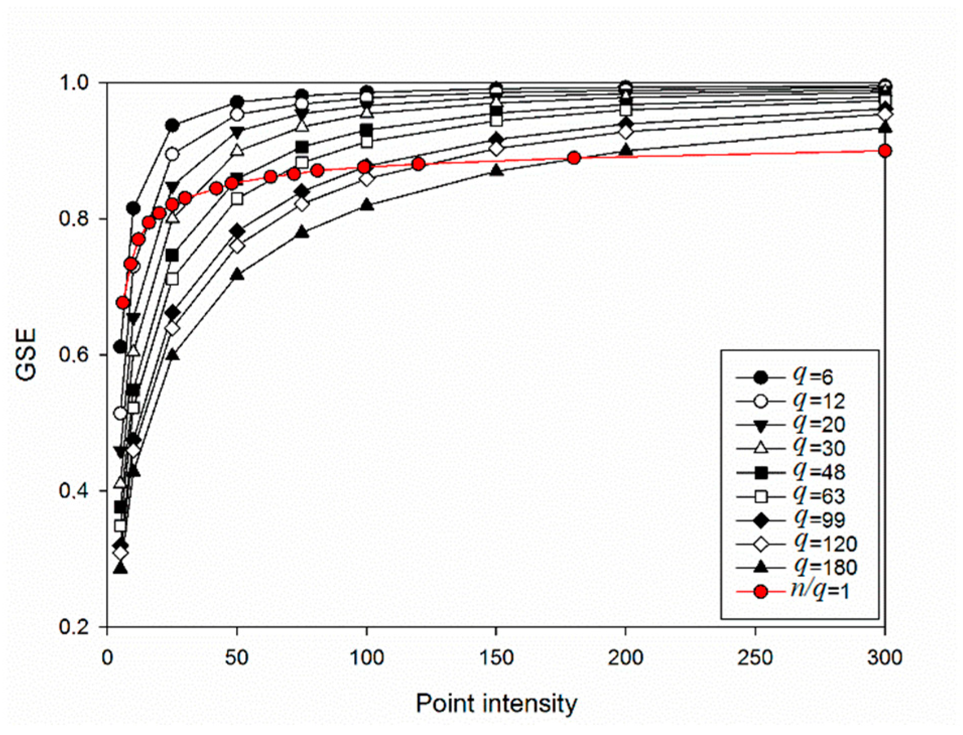
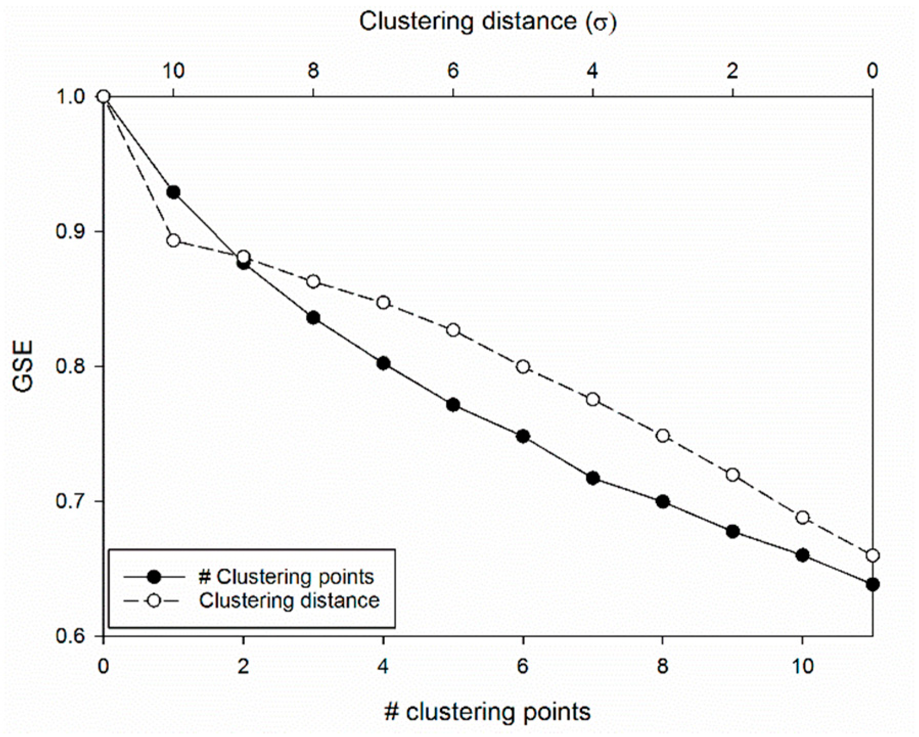
Figure 3 shows how the metric value is dependent on the amount of quadrats in the grid. This was also pointed out by Zhou et al. [16] and Kam et al. [17], and may be interpreted as an inverse density effect. The lower the q, the more points per quadrat, and the GSE increases. This dependency follows from the nature of quadrat-based metrics, and as point intensities vary, so does q. This is further illustrated in Figure 4, where the grids are seen as three images at different magnifications. In each image, n/q is constant, and keeping such a relationship should result in the most accurate results over different densities. The red curve in Figure 3 shows that keeping n/q constant reduces the variation of GSE with the point intensity. This indicates that the optimal value for q must correspond with the intensity of points in the image to minimize the “smoothening effect”. If there is a large number of quadrats, and few points in the pattern, a large number of quadrats will be empty. This will result in a low GSECSR, and the detection power of the metric will be reduced. This is likely why Zhou et al. [16] and Kam et al. [17] found that a relatively low q (9–16) was ideal for optimal detection power. However, their tests only comprised intensities of n = 30 and n = 100.
2.5. Efficiency of the GSE Metric in Detecting Non-Uniformity
Figure 5 shows the effect of changing the degree of clustering. In this example, the intensity is set to an average of n = 50 points per image. For the solid line, σ is set constant to five times the radius of the maximum dispersoid size (i.e., σ = 5, rmax = 5–150 nm), and nc is varied. For the dashed line, nc is set constant to 5, while σ is varied. The number of quadrats is set to q = 48. In both graphs, the CSR condition may be distinguished as having a GSE = 1. The non-uniformity is clearly detected by the GSE in each case, and there is a steady increase in deviation from GSECSR as non-uniformity increases. A discontinuity is seen for the graph with variable σ, as clustering with σ = 10 is still some way off CSR uniformity. Figure 5 illustrates the degree of spatial uniformity for σ = 2, 5, and 8.
2.6. A Modified GSE Metrics
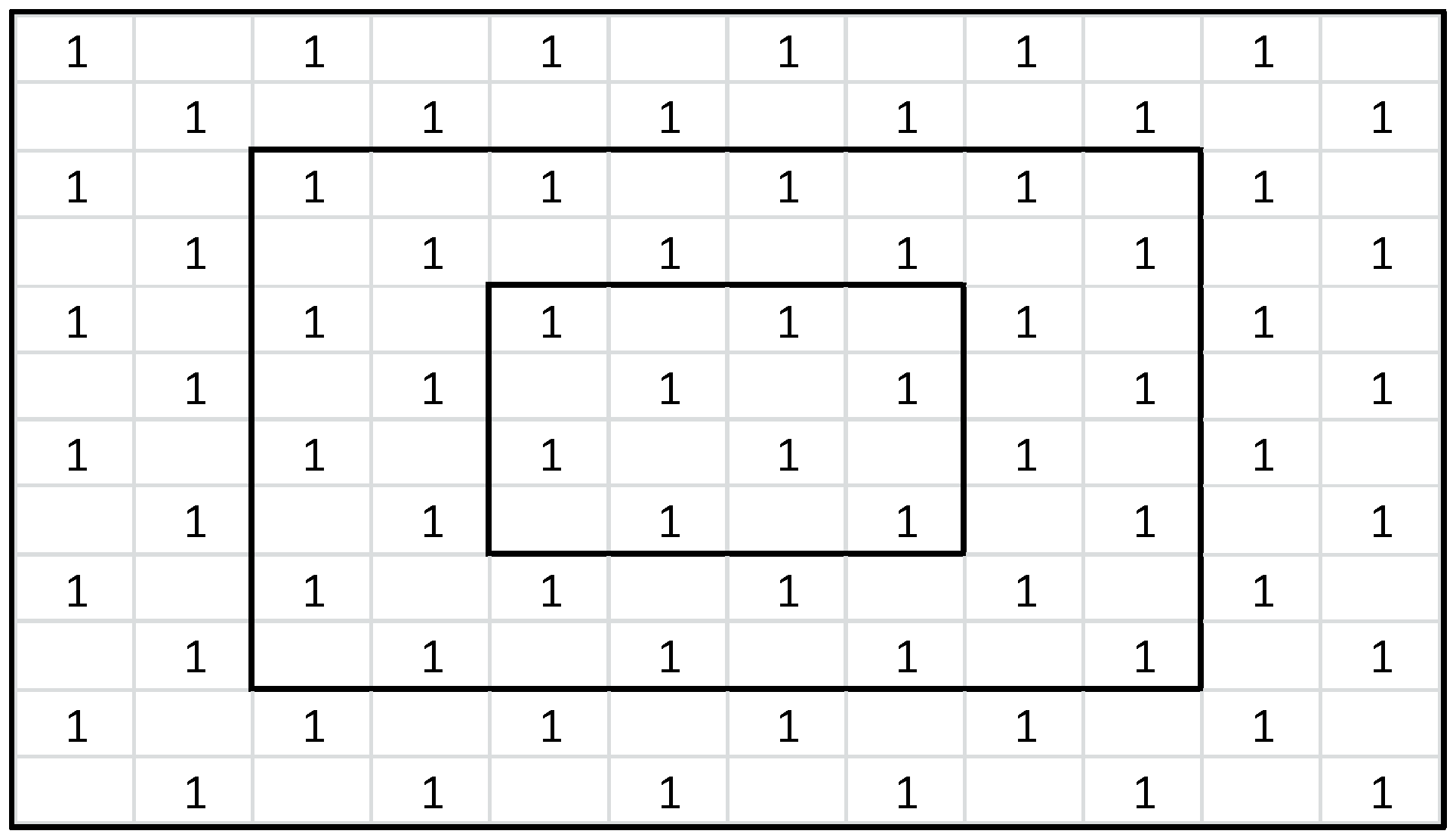
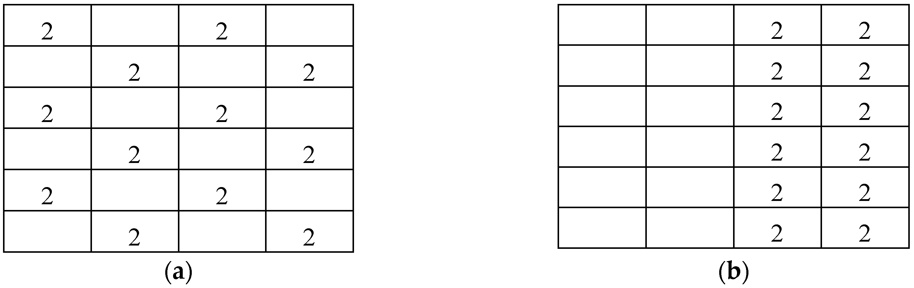
An important weakness of the GSE metric, in its original form, is that it does not provide enough spatial information. The lack of spatial information on the points inside each quadrat was mentioned in the introduction; however, there is also a lack of information about the order of the quadrats in the grid. For example, the two grids in Figure 6 represent very different spatial distributions, but the GSE metric cannot distinguish between them, and will, in both cases, result in GSE = 0.78. This is a major drawback, and likely the reason why Zhou et al. [16] and Kam et al. [17] found the metric to perform poorly at large qs. Intuitively, large qs should provide a higher resolution and therefore improved accuracy. In fact, ideally, using large enough qs should result in the resolution approaching that of distance-based metrics. However, GSE in its original form is not able to benefit from the larger amount of information available when using a higher resolution.
Metrics, which account for the location of the quadrats in the grid, are called spatial auto-correlation measures. Kam et al. [17] included four such metrics for which the Local Gi (LG) had the best detection power. However, it still scored well below the index of dispersion (ID) and the GSE, and the question is whether instead a new term may be added to the GSE to account for this problem, to combine the best of both worlds.
The new term would require the ability to determine whether quadrats with large counts are confined to certain areas in the image, and quadrats with small counts to others. A simple model of how this could be solved is described below. For high qs and under CSR conditions, the quadrats with no (or a small amount of) points will be evenly distributed. This means that moving along the rows or columns in the grid, the value of the quadrats should increase and decrease regularly. For example, in the grid in Figure 6a, moving downwards in column 1, the quadrat value will first decrease from 2 to 0, then increase to 2, before it decreases to 0 again, and so on. If there is non-uniformity, the amount of times an increase or a decrease occurs, should be lower than for CSR, as seen in Figure 6b.
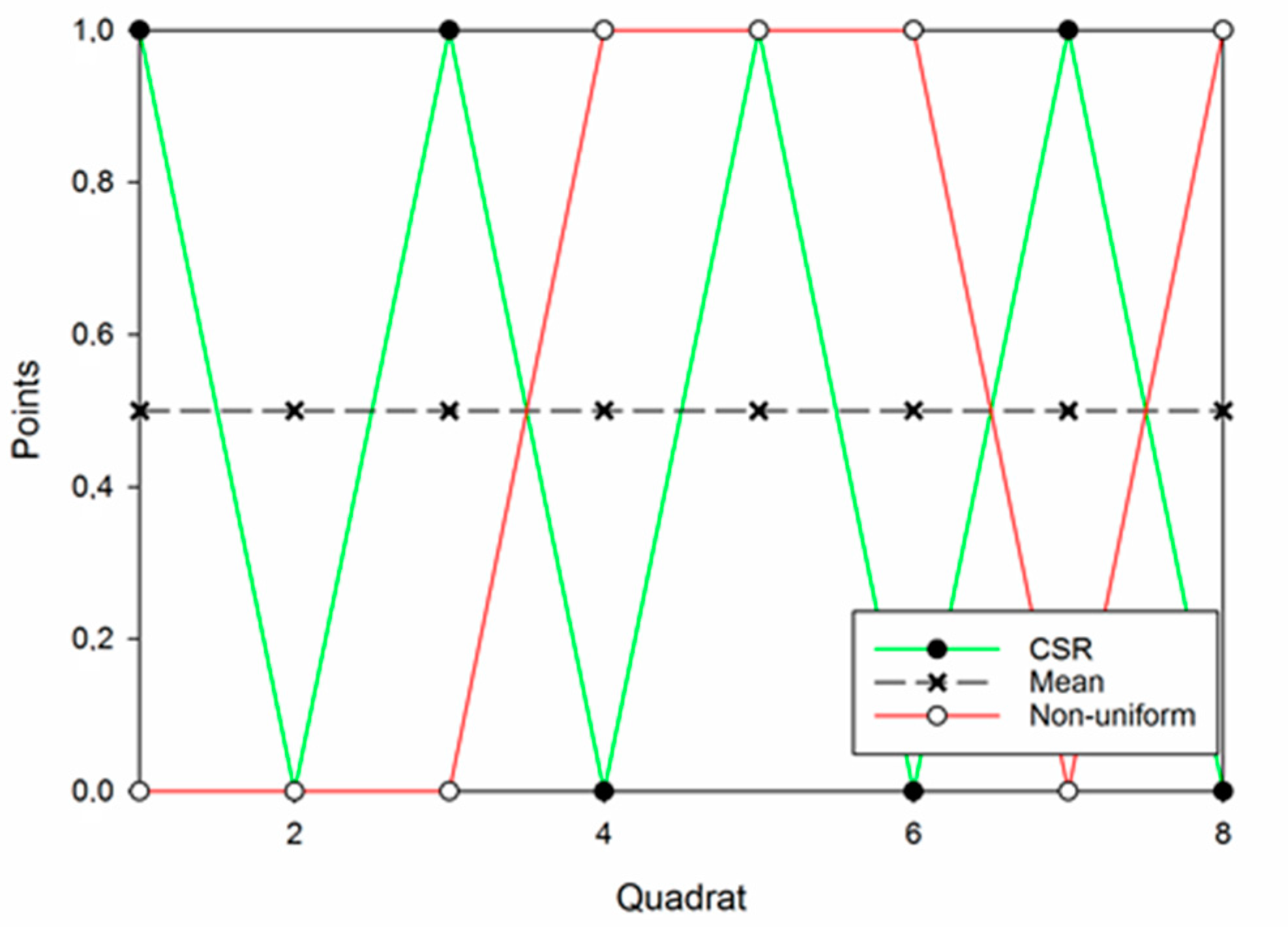
The principle may be better explained by imagining a row in an image grid. Figure 7 represents such a row, where the average intensity of points per quadrat, n/q, is equal to 0.5. In the case of CSR, the graph passes the mean seven times, while with a non-uniformity, it is only passed three times. However, in both cases, four quadrats contain one point while four are empty, so the GSE will see the patterns as equal. It is suggested that the GSE metric can be improved by including the amount of times the mean is crossed for each row and column in the grid. The new term would thus be the counts of crossings of the mean for a non-uniform pattern, normalized to that of the CSR, . A modified GSE denoted GSE* could then be described by:
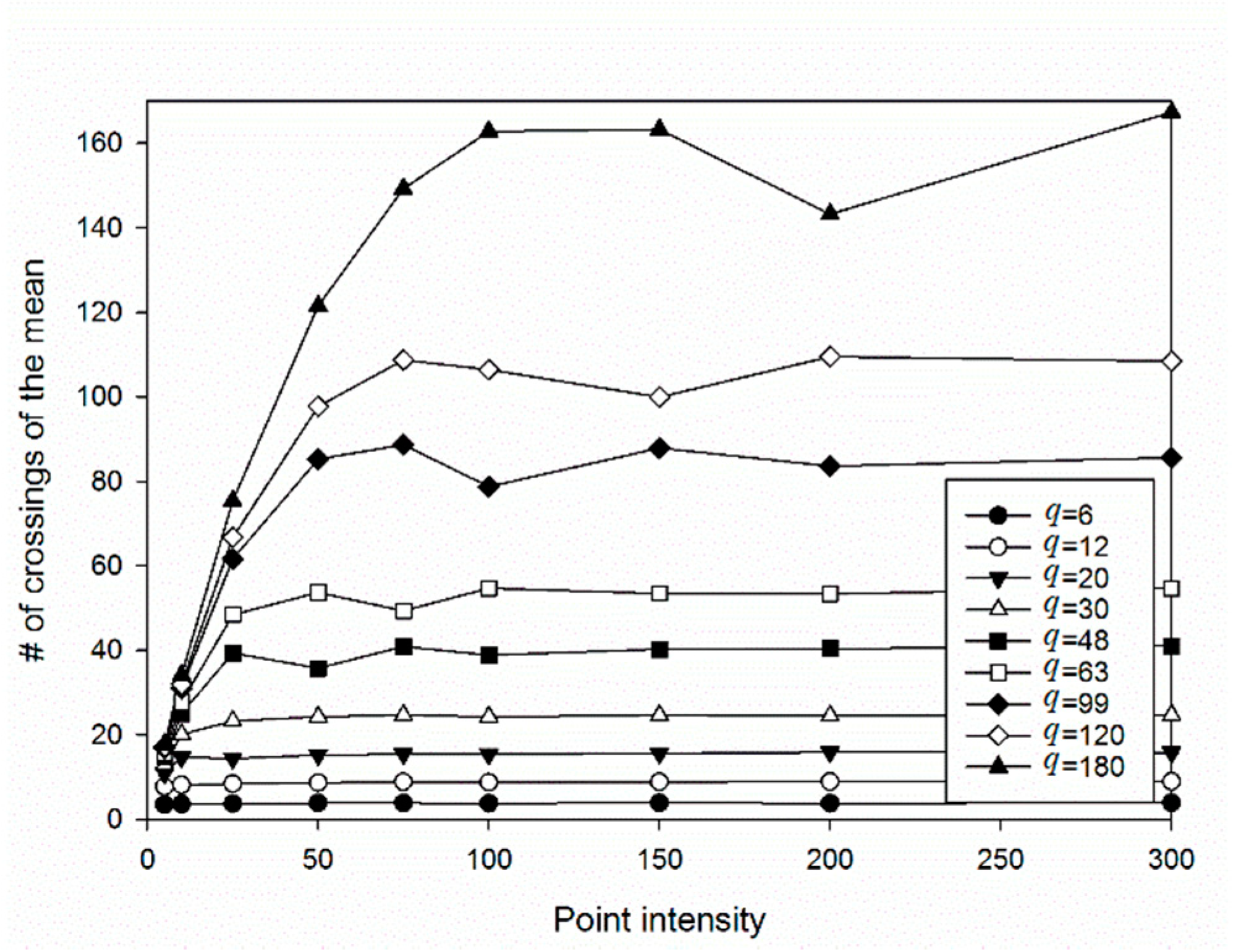
It is necessary to point out that this approach will fail if the spatial distribution approaches complete uniformity. In such a case, the graph would have a very low amount of crossings, or even none, as it would rest on (or close to) the mean. However, as was mentioned earlier, regularity rarely occurs in nature, and this should not be an issue when dealing with dispersoid distributions. Under CSR, as illustrated in Figure 7, the number of crossings increases with the intensity of points in the pattern, until it saturates at approximately half of the maximum amount of crossings possible. That is, for q = 8 × 6 = 48, the maximum amount of crossings is = 7 × 6 + 5 × 8 = 82. Thus, the number of crossings for q = 48 saturates at 41, as seen in Figure 8, and this behaviour is the same for all values of q. It is also noted that there are drops in each graph, and the drop seems to occur when the intensity of points is equal to an integer, N, multiplied by q (N × q = n, or n/q = 1, 2, 3, …). This may be related to an effect of regularity, as it then would be possible for every square to be occupied by N points, which could result in a low number of crossings.
2.7. Differentiating Degrees of Spatial Uniformity
Zhou et al. [16] were not satisfied with any of the metrics’ ability to differentiate degrees of spatial uniformity in their study. The conclusion was based on the fact that the intensity distributions of the metrics in their study overlapped for different degrees of uniformity. A metric similar to the tessellation method by Marthinsen et al. [11], for example, scored very well in terms of detection power, but for some pattern types, it had intensity distributions that were impossible to separate. However, the severity of the overlaps varied for each metric, and was the lowest for the index of dispersion (ID) and the GSE. Some overlap of the distributions is unavoidable, and it does not contradict the usefulness of the metric to provide valuable information about the degrees of uniformity. As long as they are separable, the most important indicator must be the mean of the distribution relative to the distributions of other degrees of spatial uniformity. The question is if the parameters of the metric may be optimized to provide a better separation of the distributions and the mean, and if the new term introduced in the previous section may improve the differentiation ability.
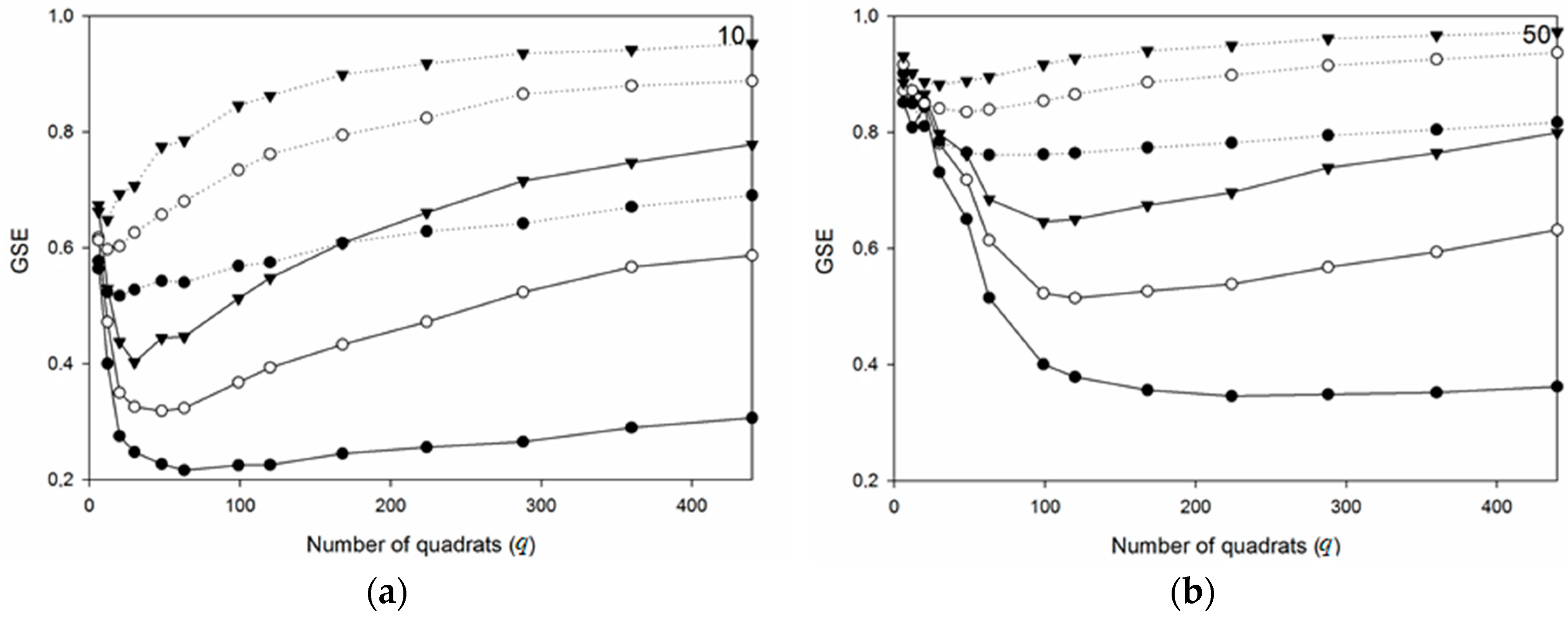
Figure 9 exemplifies four different point distributions with different degrees of clustering (non-uniformity). Figure 10a–d show the corresponding variation of the metrics, GSE and GSE*, for different point intensities, n, in each case, as a function of the number of quadrats, q. The graphs all have clusters of nc = 5, but different σ (= 2, 5, and 8). As the non-uniformity approaches CSR, it is seen that the required q for optimal detection power decreases, i.e., the minimum peak of the curves is shifted towards the smaller qs. As the patterns become more uniform for spatial distributions that approach CSR, a low q is thus necessary to detect non-uniformity. However, it is also apparent that most of the curves for the different degrees of non-uniformity separate as q increases. This means that the metric’s ability to differentiate the different spatial distributions is higher for larger qs, as long as the non-uniformity is large enough to be detected.
It is suggested that the difficulty in detecting vague non-uniformity with higher qs may be related to the problem of the relative localization of the quadrats, discussed in the previous section. The graphs of GSE* are indeed different, and seem to have a better detection power for larger qs, compared to the original GSE. Moreover, the differences between the different degrees of non-uniformity are larger, suggesting a better ability to differentiate. The new expression does, however, seem to be unstable for lower qs, indicating that larger qs in this case leads to both better stability and resolution. To reveal how the GSE and GSE* may be used in practice, an experimental study is presented in the next sections.
3. Materials and Methods
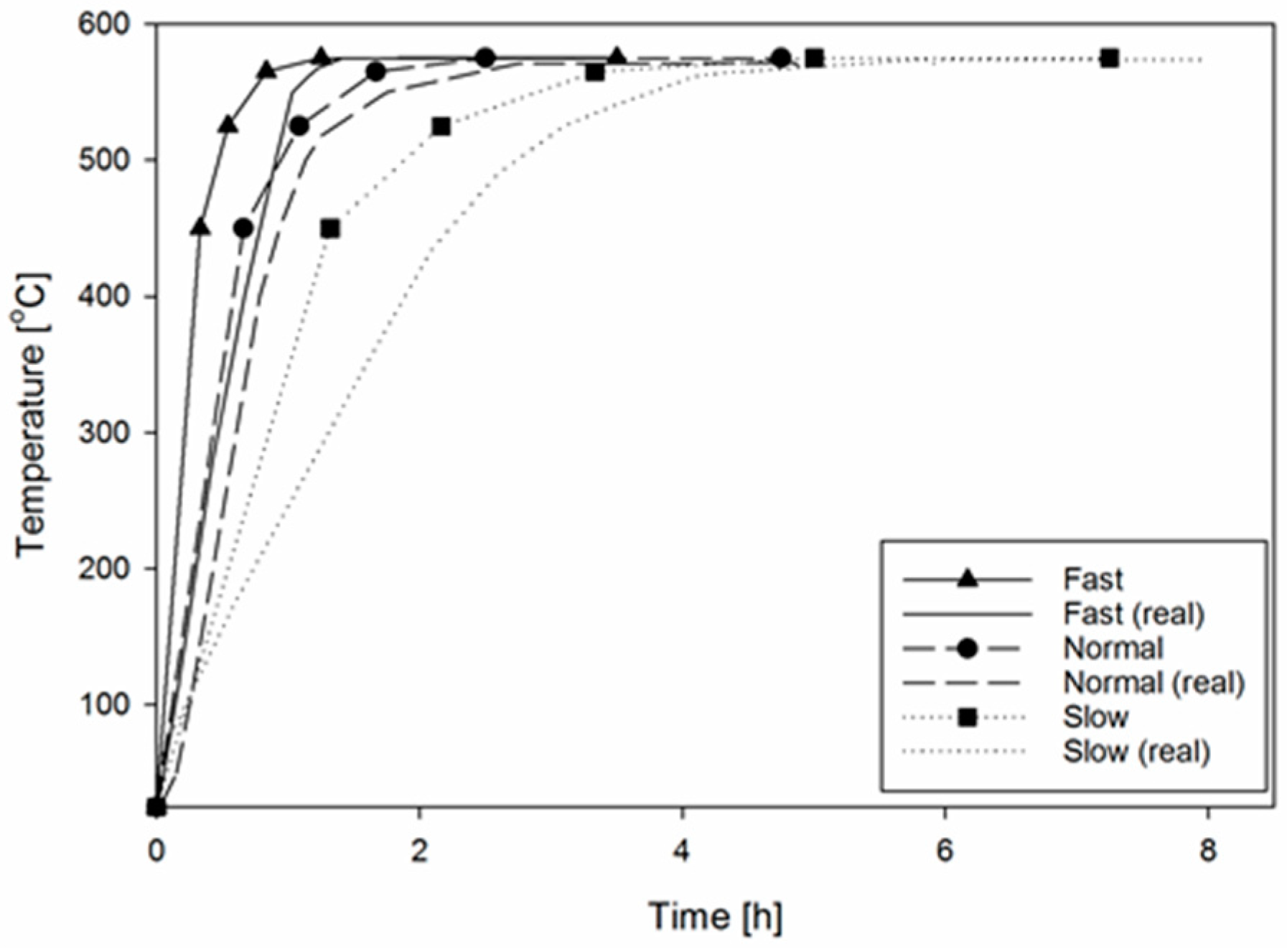
Four alloys were direct-chill (DC)-cast at Hydro (Sunndalsøra, Norway), and samples were cut out of the billets at a distance of ~3–4 cm from the centre and ~2 cm from the edge. The chemical composition of the different alloys is listed in Table 1, as determined by X-ray diffraction analysis (XRD, PANalytical Empyrean, Almelo, The Netherlands). The alloy selection was made to provide alloys (after homogenization) with different dispersoid structures, in terms of size, number density, and spatial distribution. The samples were homogenized in an air furnace (Nabertherm GmbH, Lilienthal, Germany) at a final holding temperature of 575 °C, for 2 h and 15 min. Three different heating rates were used, and all samples were water quenched upon removal. The intended homogenization cycles are found in Figure 11, along with the actual homogenization cycles logged in the furnace. The heating rate denoted “Normal” was chosen according to a typical industrial heating rate, using a five stage heating procedure set to an average of 4.6 °C/min until reaching 525 °C, and subsequently 1.0 °C/min until reaching the final temperature. The “Slow” heating rate was chosen to be the half of that of “Normal” (i.e., an average of 2.3 °C/min from 25–525 °C), while the “Fast” was set to 2 times “Normal”. As a consequence of the different heating rates, the total amount of time in the furnace was different for each heating rate.
Samples were prepared by grinding and polishing for the microstructure investigation. Dispersoid characteristics were studied in a scanning electron microscope (SEM), Zeiss Ultra 55 LE (Carl Zeiss Ag, Oberkochen, Germany). Back-scatter electron (BSE) imaging was used to obtain a Z-contrast and separate the Mn-dispersoids from the matrix. The acceleration voltage was set to 4 kV to minimize the penetration volume, and a working distance of 7.3 mm was found to be optimal for the BSE detector.
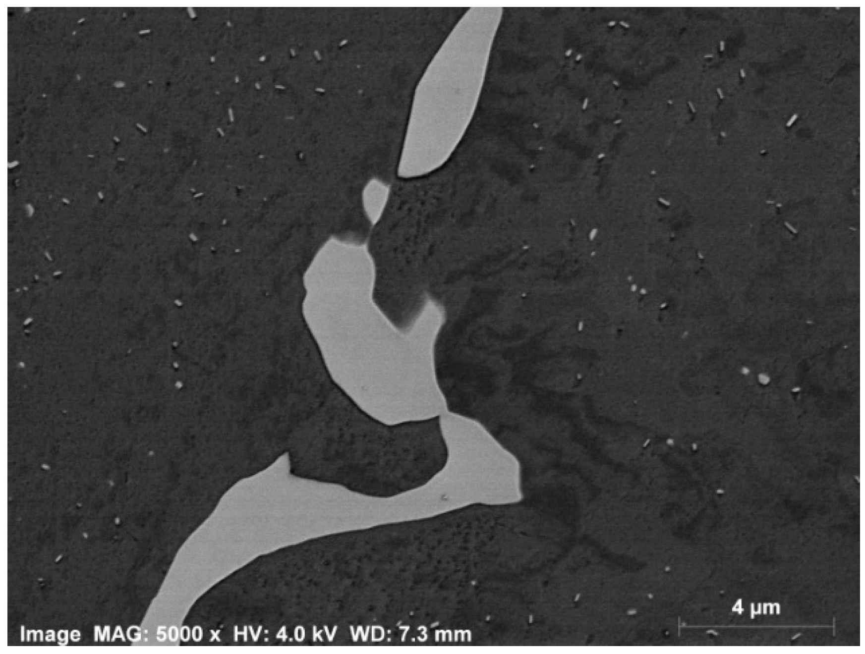
The microscope was set to the “High current” mode and an aperture of 60 µm was used to ensure a balance between a high resolution and sufficient backscatter signal. Imaging was performed in Bruker Quantax 9.4 (Bruker, Billerica, MA, USA), where the images were taken at a magnification of 5000×, and saved with a resolution of 4000 × 3000 pixels to ensure the best possible detection power. Figure 12 shows a representative BSE image from this study taken from alloy 6082. 100 such images were taken of each alloy and the heating rate and these were taken in a straight line through the samples, covering a distance of 1500 µm, and crossing approximately 18–22 grains. The total area covered was ~0.036 mm2 for each sample.
The images were analyzed in the software, IMT iSolution DT (Version 12.0, IMT i-Solution, Vancouver, BC, Canada). Thresholding was carried out manually for each image, and the final result was compared to each original image. A macro was created to return information on each dispersoid in the image, including size, position in the image (x-/y-coordinates in pixels), feret diameter, etc. Only dispersoids of sizes from 20–300 nm in diameter were accepted. Several challenges were encountered in the image analysis process. Patterns in the matrix, as seen in Figure 12, which are commonly seen in the SEM after polishing with OP-S (Oxide Polishing Solution), interfered with thresholding by making it difficult to separate the particles from the light patterns in the matrix. This problem was resolved by using the feature, “Open by area”, where one can define the minimum amount of neighbouring white pixels. Another challenge arose with the presence of dispersoids with very different sizes. Thresholding was increased to detect the smallest dispersoids, and consequently the larger particles may have been over-saturated. Areas without dispersoids, or with severe contamination, which could not be removed by thresholding, were deselected from the analyses.
Mathworks’ software, Matlab (Version 2016a, MathWorks, Natick, MA, USA), was used as the main tool to execute the different calculations in the evaluation of the GSE metric. A script was written to search through the Excel sheets with the results from iSolution, and extract the coordinates of each particle. The dispersoids were then allocated to a matrix, representing the grid of the quadrat-based method, which was explained in the previous section. Finally, the GSE was calculated based on this “grid-matrix” with the equations found in the theory.
4. Results
4.1. Number Density and Area Fraction of Dispersoids
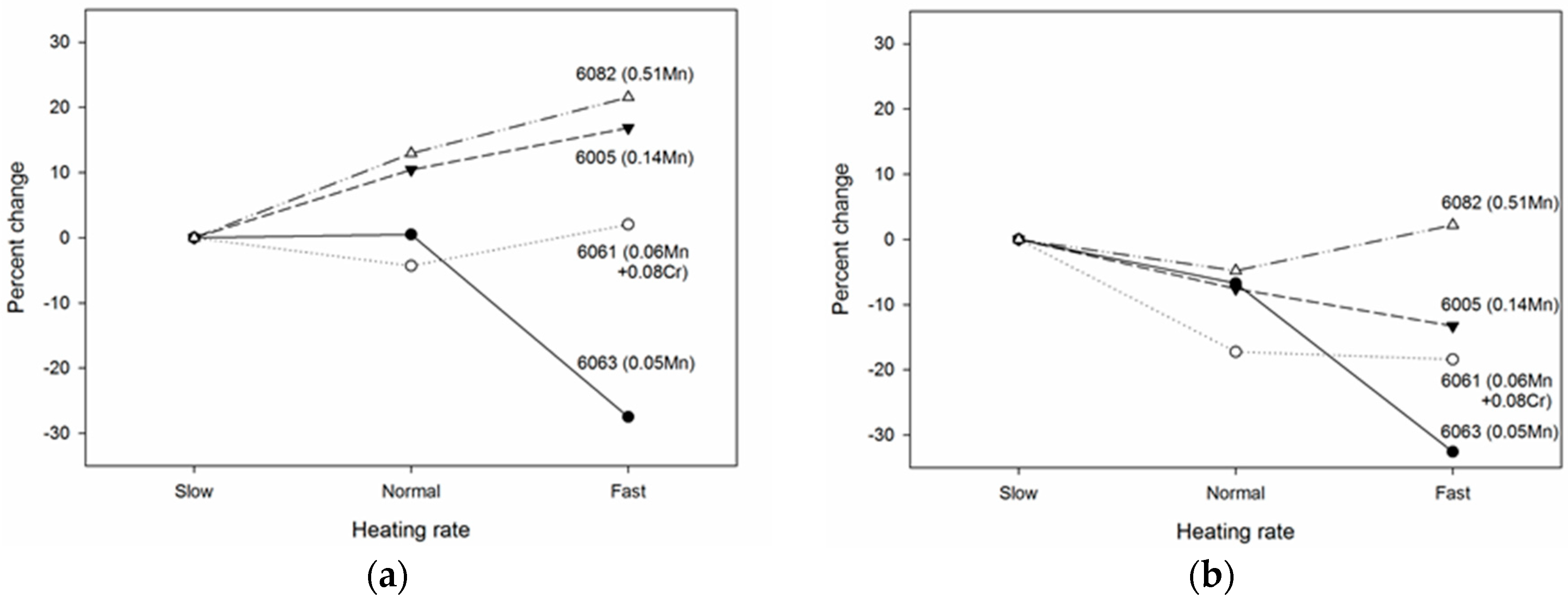
Figure 13 and Table 2 shows results for the number density and % area (i.e., percentage of area coverage) of all four alloys. Here, the “Slow” heating rate was chosen as a reference, and the variation in dispersoid density is expressed as the percent change with the increasing heating rate. No significant differences were seen in the number of density measurements for alloy 6063 when increasing the heating rate from “Slow” to “Normal”. However, increasing to the “Fast” heating rate resulted in a ~30% drop in dispersoid density. A similar development was seen for the % area measurements. With increasing heating rates, the area covered by dispersoids was also found to decrease, but this time also between “Slow” and Normal”. This behaviour of the % area was also found for alloy 6005, although less pronounced. However, for this alloy, the number density increased slightly with an increasing heating rate. Due to the higher Mn content, both larger dispersoid densities and % areas were found in this alloy, revealed by the absolute values of the dispersoid studies found in Table 2. Large variations in dispersoid density and % area between the images were also seen, expressed by the standard deviations, and indicating a non-uniform spatial distribution. The heating rate had more or less the same effect on the dispersoid density in alloys 6082 and 6005. In contrast, the % area of dispersoids in alloy 6082 remained more or less unchanged. The Cr content in alloy 6061 clearly made the dispersoid density less sensitive to differences in heating rate. The % area, however, decreased somewhat when increasing the heating rate from “Slow” to “Normal”. Finally, by examining the % area plot, it is seen that the largest percent change with increasing the heating rate was found for the leanest alloy, and the percent change decreased with increasing the alloying element content.
4.2. Size and Spatial Distribution of Dispersoids
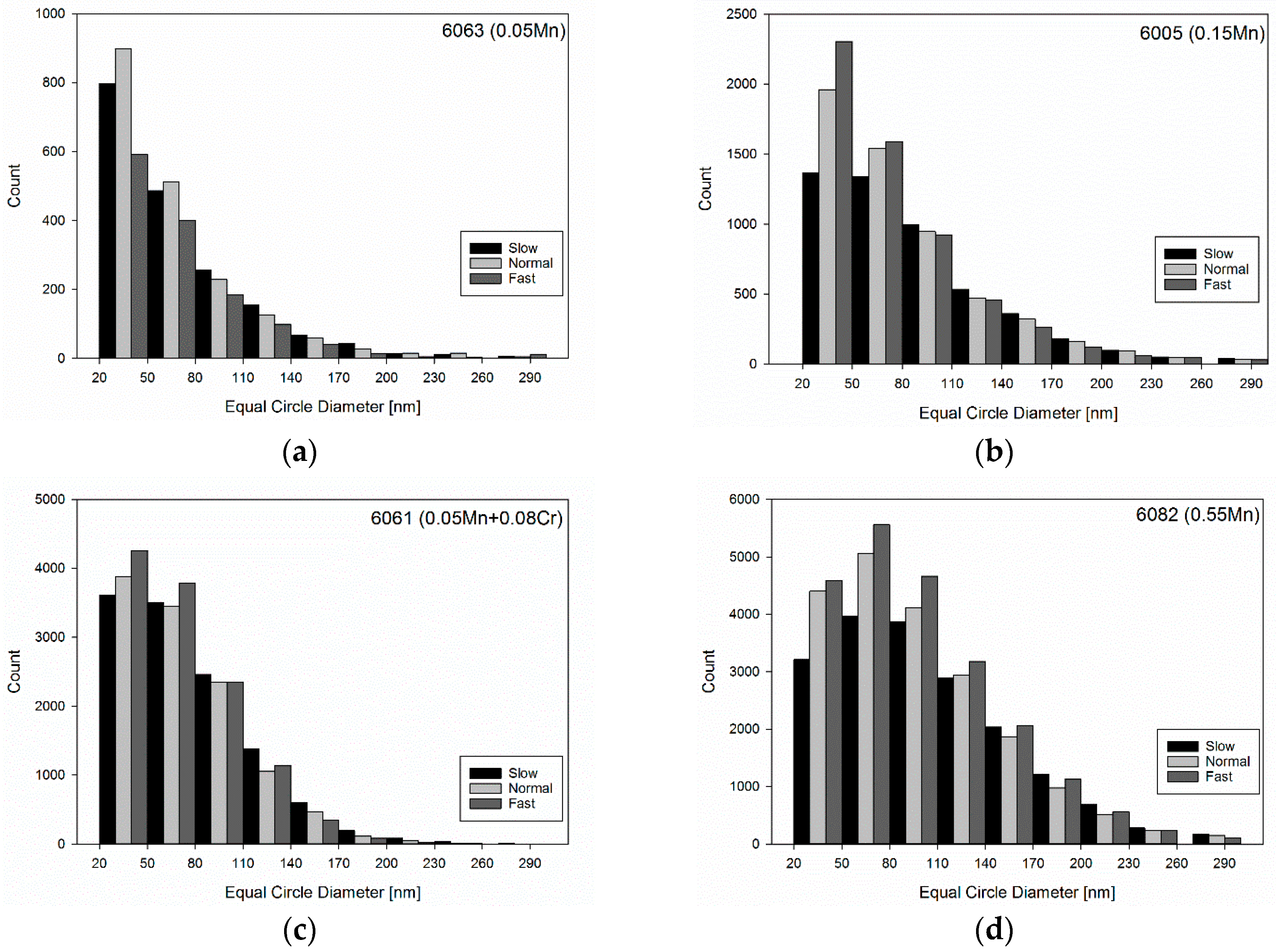
The dispersoid size distributions are presented in Figure 14. For alloys 6005, 6061, and 6082, the distribution shifted towards larger particles for slower heating rates. A “Fast” heating rate gave a larger amount of dispersoids with equivalent circle diameters (ECD) between 20–80 nm than the slower heating rates. For the larger particles, the black column, indicating the “Slow” heating rate, became dominant. This behaviour was more pronounced for alloys 6005 and 6082, which contained the highest levels of Mn.
The addition of Cr in alloy 6061 reduced the precipitation kinetics, and resulted in less coarsening of the dispersoids. The 6063 alloy displayed the same behaviour for the “Slow” and “Normal” heating rates, but a lower amount of dispersoids for all size intervals with the “Fast” heating rate.
The results concerning the spatial distribution of dispersoids, in terms of the original GSE and the modified GSE*, are presented in Table 3. Different values for q and q*, referring to GSE and GSE*, respectively, were selected based on the discussion in Section 2.7. Q was set to correspond to q/n = 1, and q* was chosen based on when the number of crossings in Figure 2 stabilized. Both GSE and GSE* showed a clear decrease with an increasing heating rate for alloys 6063 and 6005, but the modified metric showed lower values than the original GSE. For 6061 and 6082, the trends were not clear. The GSE and GSE* for the 6061 alloy seemed to decrease, but the trend was very weak. The same trend, however, was observed in the relative standard deviation, , showing the variation between the images, though also weak. Finally, 6082 showed no trend as the “Normal” heating rate resulted in the poorest spatial distribution.
In addition to the GSE and GSE*, which return results about the spatial distribution inside the images, it may be useful to assess the variation in density between the images. A measure for this is the relative standard deviation, which increased with increasing non-uniformity, and is also found in Table 3. It corresponded quite well with the results from the GSE analysis, and is thus an independent metric that supports these results of the GSE and GSE*.
5. Discussion
5.1. Density and % Area
The first objective of the present study was to establish a reliable method for the characterization of the density and area fraction of dispersoids by SEM, and to evaluate how they evolve as a function of the heating rate. The quantitative analysis of particles from images is often a challenge, where one must make judgements on what features belong to the class of interest, and which do not. Due to the small sizes of dispersoids, both sample preparation and thresholding require the utmost care, but even then, some contamination is unavoidable, which may affect the accuracy. However, with the measures taken in the sample preparation and image processing, contamination of OP-S on the sample surface was negligible, and the absolute values for the number densities are deemed reliable. On the other hand, the absolute values for the % area and particle sizes are more uncertain.
From Table 2, it is seen that the results for the % area did not correspond well with the Mn-/Cr-content. Assuming α-Al(FeMn)3Si as the reigning dispersoid phase, the modelling software, Alstruc (Version 2016, SINTEF, Trondheim, Norway) [20,21], estimated the % volume fraction of dispersoids as 0.04 (6063), 0.05 (6005), 0.06 (6061), and 0.12 (6082). As the images cover several were be considered interchangeable. This is generally considered to be a good assumption if the particles are (near) spherical and the spatial distribution is not too far from random, which was the case for our samples. In this regard, alloy 6063 showed a reasonable % area, with values ranging between 0.019–0.027. However, the other alloys showed values for the % area that were two to three times larger than the modelling results indicate. Alstruc gave only an estimate of the volume fraction, and some dispersoids were likely different phases than α-Al(FeMn)3Si. However, these factors were expected to have a limited effect on the results. The most likely explanation for this behavior is that it comes as an effect of the experimental penetration volume. Although a low acceleration voltage in the SEM was used, a certain penetration volume is unavoidable, and will result in the inclusion of areas slightly under the sample surface. This effect may be more pronounced for larger particles, as parts of the dispersoids just below the surface may be included. Furthermore, the sample preparation with OP-S gives a slight etch around the Mn-/Cr- particles, which results in a shallow “ditch” around the dispersoids, indicating a larger area than the real value. An alternative is to use transmission electron microscopy (TEM), but that gives problems with statistics, and is not within the scope of this study.
Precipitation kinetics typically increases with super-saturation, and is expressed by the % area. It is therefore reasonable to assume that there should be a relationship between the alloying content and changes in % area as the heating rate is changed. Mn and Cr have low diffusivities in aluminium, and as the atoms may have to travel long distances to nucleate, the heating rate, or rather, the amount of time spent at higher temperatures, may be more critical than for alloys with a higher Mn content. This was clearly expressed in Figure 13b, where the graphs distinctly align according to the alloying content. The plot thus gives an indication of how much Mn and Cr was precipitated. As the 6082 alloy showed small variations, it is reasonable to assume that, for this alloy, Mn was more or less fully precipitated for all heating rates. This was not the case for the other alloys, however, and especially 6063 did not fulfilled its nucleation potential of Mn for the faster heating rates.
Upon commencing these experiments, it was expected to find that number densities would be influenced by the heating rate in a manner similar to what was seen for the 6063 alloy in Figure 13a. Here, the dispersoid density was higher for lower heating rates. This expectation was based on earlier studies, which showed an increase in dispersoid number densities with decreasing homogenization temperatures [10,22]. Such a relation suggests that the amount of time spent at lower temperatures could lead to an increase in number density. This also fits well with Lodgaard and Ryum’s work [8] on the precipitation behaviour of these particles. Assuming that the reigning precipitation mechanism is via intermediate phases precipitated at lower temperatures, it is reasonable to expect that a high density of the intermediate phases should result in a high density of the final dispersoid phase(s).
For 6063, there was a ~30% difference in number density between the “Normal” and “Fast” heating rates while there was no significant difference between “Slow” and “Normal”. This suggests that there exists a ‘critical heating’ rate or temperature range for optimal nucleation. However, this critical region is unlikely to be at lower temperatures, since the temperature logs in the furnace showed that it was not possible to heat the samples at a higher rate than “Normal” in the first heating stage. This means that the heating rate for “Normal” and “Fast” were practically the same until reaching ~450 °C. The change in number density must therefore mainly be the result of occurrences after this stage. According to Lodgaard et al. [8], precipitation of Mn starts through the precipitation of an intermediate “u-phase” around 350–400 °C, before dispersoids were nucleated on this phase from ~400 °C. If this is the case, the current results suggest that the nucleation of the “u-phase” and Mn-dispersoids was the critical stage for alloy 6063, and that the final density of dispersoids may be less, or not at all, influenced by the precipitation of β’ at lower temperatures. However, this hypothesis is based solely on the assumption that Lodgaard’s model was dominant [8], and one must keep in mind that there may also be other precipitation mechanisms operating.
Interestingly, 6005 was found to behave in a rather different manner. In contrast to 6063, the number density increased by ~20% when increasing the heating rate from “Slow” to “Fast”. An explanation for this behaviour arises from the likely differences in super-saturation of Mn, Mg, and Si in the two alloys. It is suggested that, due to the higher alloying content in the 6005 alloy, the diffusion distances were shorter, and consequently nucleation and growth occurred easier. The nucleation nose (in a TTT-diagram) was shifted towards shorter times, and was fully entered also by the heating curve for the “Fast” heating rate. This is supported by the results from the denser alloy 6082, which showed the same behaviour, only more prominent.
The dispersoid density of the Cr-containing 6061 alloy was unaffected by the changes in the heating rate. This is likely due to the different nucleation temperatures for Mn and Cr. Cr-dispersoids nucleate at higher temperatures than Mn-dispersoids, and since the super-saturation of Cr was quite low, the precipitation was likely to be slow below 500 °C. Electrical conductivity measurements by Lodgaard and Ryum [23] gave a dip around 530 °C for a 0.15 wt % Cr alloy, while the dip occurred around 490 °C for a 0.32 wt % Cr alloy. As the 6061 alloy contained 0.08 wt % Cr and 0.06 wt % Mn, precipitation should start around 530 °C. This reasoning also supports the interpretation of the number density results of 6063. With a Mn-content of only 0.05 wt %, the dispersoid precipitation in 6063 is likely to occur at significantly higher temperatures than for 6005 and 6082, which agrees with the assumption that the 30% drop in number density must have resulted from temperatures above 450 °C. This behavior suggests that the “Fast” heating rate of 6063 must have passed a nucleation nose too fast to fulfil the nucleation potential of Mn. Why a change in number density was not seen for the 6061 alloy may be due to the differences in the heating rate above 530 °C being too small to give a significant effect, or perhaps that a slight difference in nucleation density was compensated for by a competing coarsening of the dispersoid phases for slower heating rates.
Figure 14 clearly shows a particle distribution shifted towards coarser particles for decreasing heating rates in 6005, 6061, and 6082. This behavior was already suggested by Figure 13a, which showed a lower number density for decreasing heating rates in 6005 and 6082. The “Slow” heating was found to give a significantly lower amount of dispersoids between 20–80 nm than what was found for other two heating rates. The alloy in this case also contained a slightly larger amount of particles in the size ranges above 80 nm. Together, these plots indicate increased Oswald ripening as the heating rate was reduced. The same behaviour was seen for 6063 with the “Slow” and “Normal” heating rate. However, the “Fast” heating rate was strongly shifted towards larger particles. That is, the bars for the two smallest particle size intervals were now significantly lower as compared to the other heating rates, while the bars for the larger particles fitted with the trend. This result clearly agrees with the suggestion that nucleation was limited for the “Fast” heating rate, but that growth at higher temperatures proceeded normally.
It has been reported that Cr-dispersoids coarsen more slowly than Mn-dispersoids [7], and the particle size distribution in Figure 14 agrees with this. It was clearly shifted towards smaller sizes than for the Mn alloys, and the absolute dispersoid density was also much higher with respect to the alloying content. Moreover, Figure 13b shows a 20% difference in % area when comparing the “Slow” and “Normal” heating rates. The “Slow” heating rate results in approximately 1 h and 15 min more above 500 °C than the “Normal”, and suggests that sufficient time above this temperature range was crucial for complete precipitation with such a low Cr and Mn content.
5.2. Spatial Distribution (GSE)
The second objective of the current study was to assess methods for evaluating the spatial distribution of dispersoids. Several methods have been developed, but many of these are not sufficiently precise or easy to implement. An attractive feature of the GSE is its simplicity. It only requires point coordinates or the count in each square of the grid, and the rest can be automated. The choice of using the quadrat-based method was based partly on convenience, but of course, also on efficiency. The GSE proved to have the most efficient detection power in the studies by Zhou et al. [16] and Kam et al. [17], but also gave indications of an ability to differentiate degrees of spatial uniformity [16]. The latter was dismissed by Zhou et al. [16] due to overlapping intensity distributions; these were, however, only partially overlapping for the GSE, and could clearly be distinguished from each other. The conclusion was based on an interest in evaluating whether one image has a certain spatial distribution, and this is not a relevant concern in the present study. At high magnifications, such as those needed when studying dispersoids, both density and spatial distribution may vary significantly from image to image, and the main concern is thus whether a sample population of images differs from another. It should be noted that the size of the particles is not accounted for by the GSE-metric. As the dispersoids are small compared to the sample area, this is, however, not an issue in the present work.
Figure 5 shows how the GSE metric consistently picks up the differences in spatial distribution as the cluster parameters were gradually changed. This indicates that the GSE could differentiate the spatial uniformity of sample populations. However, the graph, for which only σ was changed (open symbols) shows that the ability to differentiate decreased as the spatial distribution approached uniformity. This is also what was pointed out by Zhou et al. [16], where the largest overlaps were seen close to CSR. However, the effect of each incremental change of σ on uniformity became smaller as σ increased. This characteristic of the graph was thus a result of small changes in the spatial distribution and was not caused by problems with the metric. Although this is true, it is also obvious that the necessity to differentiate spatial uniformity disappears as it approaches uniformity.
A problem appears, however, when the point intensity was large. This is seen in Table 3, where the GSE of 6082 was almost 1. By visual inspection of the images, e.g., in Figure 12, it is obvious that this cannot be accurate. The question is whether GSE* can improve the sensitivity of the metric. This effect was already seen in Figure 10, where the graphs are more spaced than for the GSE. Moreover, this is again expressed in Table 3, where GSE* showed the same trend as for the GSE, but with lower values. It also seems to pick up information in the analyses of 6061 and 6082 that GSE cannot, however, these results are ambiguous.
In Table 3, the trend seems to be the same for both the original and the modified GSE. In general, the GSE and the GSE* scores higher for slower heating rates, indicating a more uniform spatial distribution. Earlier studies have found the spatial distribution of both Cr- and Mn-containing alloys to be dependent on the heating rate [12]. In general, both a slower heating rate, and a lower homogenisation temperature seem to promote a more uniform spatial distribution [8,12,23]. In Lodgaard and Ryum’s studies [12], Cr-containing alloys required a slower heating rate than the Mn-containing alloys, and the critical heating rates for a homogeneous spatial distribution were far above the one’s used in the current study. However, the alloys used were also much denser, and this may have a significant effect. According to Table 3, both the GSE and the GSE* decreased steadily with an increasing heating rate for the two low-Mn alloys, 6063 and 6005. Moreover, the relative standard deviation of the density between the images was very high in each condition, and showed the same trend towards a more non-uniform spatial distribution for faster heating rates. The 6061 alloy seems to have a weaker trend than the above mentioned, and indicates that the higher precipitation temperature or slower diffusivity of the Cr-containing alloy makes the dispersoid density and spatial distribution less sensitive to changes in the heating rate for the alloy compositions in question. The results from the 6082 alloy are more difficult to interpret, and are somewhat different for GSE and GSE*. There is no clear trend, but there was quite a big difference between the GSE and the GSE* results.
6. Conclusions
On the basis of the findings in this study, the following may be concluded. The dispersoid density, particle size distribution, and spatial distribution for Al-Mg-Si alloys with a low Mn content were affected by the heating rate to the homogenization temperature. An increase in dispersoid number density and a more uniform distribution of dispersoids was found for the lowest heating rate, as compared to the more rapid heating rates, for the alloy with 0.05 wt % Mn. This is suggested to be due to shorter times in the temperature range for precipitation of Mn-dispersoids. For the alloy with 0.15 wt % Mn, it was found that the number density increases with the heating rate. This is suggested to be due to particle coarsening as an effect of the samples spending a longer time in the furnace with the low heating rate.
Concerning the possibilities and ability to characterize the spatial distribution of dispersoids, it can be concluded that the Global Shannon Entropy (GSE) metric, with a careful selection of relevant parameters, is an adequate metric for the detection of non-uniformity of dispersoid structures in Al-Mg-Si-alloys. Moreover, with the new term it was demonstrated that the ability to differentiate the degrees of spatial uniformity was improved.
Both GSE and GSE* show a clear decrease with an increasing heating rate for alloys AA6063 and AA6005, where the trend was most obvious with the modified metric (GSE*). For AA6061 and AA6082, the trends in terms of GSE/GSE* were not clear, although a weak decrease was indicated for both alloys.
Author Contributions
M.S.R. performed all the experimental work, implemented and made the analysis by and application of the GSE metric, and drafted the manuscript. I.W. and K.M. contributed to analyses and discussions of the results and to writing and editing of the manuscript.
Funding
This research work was funded by the Research Council of Norway (RCN) and the Industrial partner Hydro Aluminium through the competence building project (RCN project number: 193179/I40) in Norway.
Acknowledgments
Hydro Aluminium is greatly acknowledged for providing the alloys in this study.
Conflicts of Interest
The authors declare no conflict of interest.
References
- Kuijpers, N.C.W.; Vermolen, F.J.; Vuik, C.; Koenis, P.T.G.; Nilsen, K.E.; van der Zwaag, S. The dependence of the beta-AlFeSi to alpha-Al(FeMn)Si transformation kinetics in Al-Mg-Si alloys on the alloying elements. Mater. Sci. Eng. A 2005, 394, 9–19. [Google Scholar] [CrossRef]
- Bischel, H.; Reid, A.; Langerweger, J. Metallographic investigation of the influence of small additions of manganese to AlMgSi0.5 alloys. Aluminium 1981, 57, 787–791. [Google Scholar]
- Lohne, O.; Dons, A.L. Quench sensitivity in AlMgSi-alloys containing Mn or Cr. Scand. J. Metall. 1983, 12, 34–36. [Google Scholar]
- Bryant, A.J.; Rise, E.; Field, D.J.; Butler, E.P. Al-Mg-Si Extrusion Alloy and Method. European Patent EP0222479B1, 6 September 1989. [Google Scholar]
- Reiso, O.; Ryum, N.; Strid, J. Melting of secondary-phase particles in AlMgSi alloys. Metall. Trans. A 1993, 24, 2629–2641. [Google Scholar] [CrossRef]
- Reiso, O. Extrusion of AlMgSi Alloys; Materials Forum; Institute of Materials Engineering Australasia Ltd.: Melbourne, Australia, 2004; pp. 32–46. [Google Scholar]
- Sheppard, T. Extrusion of Aluminium Alloys; Kluwer Academic Publishers: Hingham, MA, USA, 1999. [Google Scholar]
- Lodgaard, L.; Ryum, N. Precipitation of dispersoids containing Mn and/or Cr in Al-Mg-Si alloys. Mater. Sci. Eng. A 2000, 283, 144–152. [Google Scholar] [CrossRef]
- Cai, M.; Robson, J.D.; Lorimer, G.W. Simulation and control of dispersoids and dispersoid-free zones during homogenizing an AlMgSi alloy. Scr. Mater. 2007, 57, 603–606. [Google Scholar] [CrossRef]
- Pettersen, T.; Li, Y.J.; Furu, T.; Marthinsen, K. Effect of changing homogenization treatment on the particle structure in Mn-containing aluminium alloys. In Recrystallization and Grain Growth III, Pts 1 and 2; Kang, S.J.L., Huh, M.Y., Hwang, N.M., Homma, H., Ushioda, K., Ikuhara, Y., Eds.; Trans Tech Publications: Zurich, Switzerland, 2007; Volume 558–559, pp. 301–306. [Google Scholar]
- Marthinsen, K.; Daaland, O.; Furu, T.; Nes, E. The spatial distribution of nucleation sites and its effect on recrystallization kinetics in commercial aluminum alloys. Metall. Mater. Trans. A 2003, 34A, 2705–2715. [Google Scholar] [CrossRef]
- Lodgaard, L.; Ryum, N. Distribution of Mn- and Cr-containing dispersoids in Al-Mg-Si-alloys. In Aluminium Alloys: Their Physical and Mechanical Properties, Pts 1-3; Starke, E.A., Sanders, T.H., Cassada, W.A., Eds.; Institute of Materials Engineering Australasia Ltd.: Melbourne, Australia, 2000; Volume 331–333, pp. 945–950. [Google Scholar]
- Avrami, M. Kinetics of Phase Change. I General Theory. J. Chem. Phys. 1939, 7, 1103–1112. [Google Scholar] [CrossRef]
- Avrami, M. Kinetics of Phase Change. II Transformation-Time Relations for Random Distribution of Nuclei. J. Chem. Phys. 1940, 8, 212–224. [Google Scholar] [CrossRef]
- Avrami, M. Granulation, Phase Change, and Microstructure Kinetics of Phase Change. III. J. Chem. Phys. 1941, 9, 177–184. [Google Scholar] [CrossRef]
- Zhou, Q.; Zeng, L.; DeCicco, M.; Li, X.; Zhou, S. A comparative study on Clustering Indices for Distribution Uniformity of Nano-particles in Metal matrix Nano-composites. CIRP J. Manuf. Sci. Technol. 2012, 5, 348–356. [Google Scholar] [CrossRef]
- Kam, K.M.; Zeng, L.; Zhou, Q.; Tran, R.; Yang, J. On assessing spatial uniformity of particle distributions in quality control of manufacturing processes. J. Manuf. Syst. 2013, 32, 154–166. [Google Scholar] [CrossRef]
- Cressie, N. Statistics for Spatial Data; John Wiley & Sons: Hoboken, NJ, USA, 1993. [Google Scholar]
- Diggle, P.J. Statistical Analysis of Spatial and Spatio-Temporal Point Patterns, 3rd ed.; Chapman and Hall: London, UK, 2013. [Google Scholar]
- Dons, A.L.; Jensen, E.K.; Langsrud, Y.; Tromborg, E.; Brusethaug, S. The Alstruc microstructure solidification model for industrial aluminum alloys. Metall. Mater. Trans. A 1999, 30, 2135–2146. [Google Scholar] [CrossRef]
- Dons, A.L. The Alstruc homogenization model for industrial aluminium alloys. J. Light Met. 2001, 1, 133–149. [Google Scholar] [CrossRef]
- Strobel, K.; Sweet, E.; Easton, M.; Nie, J.F.; Couper, M. Dispersoid Phases in 6xxx Series Aluminium Alloys. In Pricm 7, Pts 1-3; Nie, J.F., Morton, A., Eds.; Institute of Materials Engineering Australasia Ltd.: Melbourne, Australia, 2010; Volume 654–656, pp. 926–929. [Google Scholar]
- Lodgaard, L.; Ryum, N. Precipitation of chromium containing dispersoids in Al-Mg-Si alloys. Mater. Sci. Technol. 2000, 16, 599–604. [Google Scholar] [CrossRef]
Figure 1.
Examples of a complete spatial random (CSR) pattern (a) and a non-uniform matern cluster pattern (b).
Figure 1.
Examples of a complete spatial random (CSR) pattern (a) and a non-uniform matern cluster pattern (b).

Figure 2.
Illustration of (a) quadrat-based methods and (b) distance-based methods. Reproduced from [17], with permission from Elsevier, 2013.
Figure 2.
Illustration of (a) quadrat-based methods and (b) distance-based methods. Reproduced from [17], with permission from Elsevier, 2013.

Figure 3.
Dependency of the Global Shannon Entropy (GSE) metric on point intensity (ni) and number of quadrats (q).
Figure 3.
Dependency of the Global Shannon Entropy (GSE) metric on point intensity (ni) and number of quadrats (q).

Figure 4.
An example of q’s relationship with density, n. As the point intensity decreases, an accompanying decrease in grid size is required to give the same spatial distribution. However, due to the “smoothening effect”, the GSE increases slightly with increasing point intensity also in this example.

Figure 5.
The variation of GSE with the number of clustering points (σ = constant; filled symbols) and the standard deviation of the distribution of clustering points (nc = constant; clustering distance (open symbols). Conditions close to CSR will only occur at σ » 10, leading to the discontinuity for the clustering distance graph at σ = 10. In both cases, q has been set constant to 6 × 8 = 48.

Figure 6.
Two spatial point patterns that the GSE parameter is not able to differentiate. (a) Uniform distribution, (b) completely partitioned.
Figure 6.
Two spatial point patterns that the GSE parameter is not able to differentiate. (a) Uniform distribution, (b) completely partitioned.

Figure 7.
An example of a row in a grid under CSR and non-uniform conditions.

Figure 8.
The count of crossings of the mean as a function of point intensity. The drop in the plot may be due to this being the optimal q for the specific point intensity (see text).
Figure 8.
The count of crossings of the mean as a function of point intensity. The drop in the plot may be due to this being the optimal q for the specific point intensity (see text).

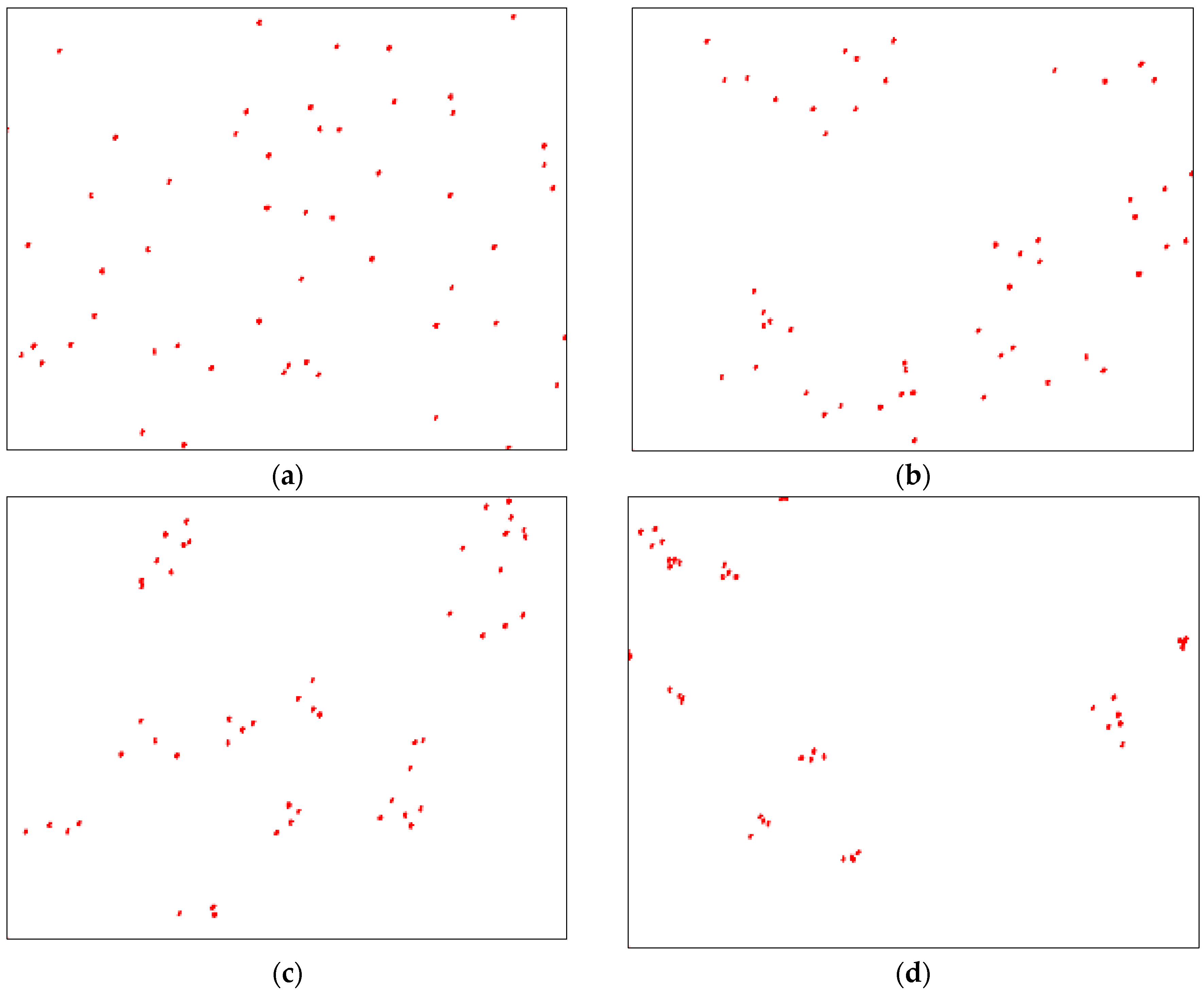
Figure 9.
Examples of the spatial point distributions generated and tested in Figure 4, with (a) CSR, (b) σ = 8, (c) σ = 5, and (d) σ = 2.
Figure 9.
Examples of the spatial point distributions generated and tested in Figure 4, with (a) CSR, (b) σ = 8, (c) σ = 5, and (d) σ = 2.

Figure 10.
The effect of q on the deviation from CSR. The different graphs represent different degrees of clustering, with σ = 2 being closest to CSR. (a) n = 10, (b) n = 50, (c) n = 120, (d) n = 180. Stippled lines: original GSE. Solid lines: modified GSE*.
Figure 10.
The effect of q on the deviation from CSR. The different graphs represent different degrees of clustering, with σ = 2 being closest to CSR. (a) n = 10, (b) n = 50, (c) n = 120, (d) n = 180. Stippled lines: original GSE. Solid lines: modified GSE*.


Figure 11.
Temperature plots of the intended and the logged (real) homogenization cycles.

Figure 12.
An example of a back-scatter electron scanning electron microscopy (BSE SEM) image of the dispersoid assessments. The image is taken from alloy 6082 after homogenization with a slow heating rate.
Figure 12.
An example of a back-scatter electron scanning electron microscopy (BSE SEM) image of the dispersoid assessments. The image is taken from alloy 6082 after homogenization with a slow heating rate.

Figure 13.
Percent change in dispersoid number density (a) and % area (b) as a function of the heating rate.
Figure 13.
Percent change in dispersoid number density (a) and % area (b) as a function of the heating rate.

Figure 14.
Particle size distribution as a function of heating rate. (a) 6063, (b) 6005, (c) 6061, (d) 6082. Note the different scales along the ordinate axes.
Figure 14.
Particle size distribution as a function of heating rate. (a) 6063, (b) 6005, (c) 6061, (d) 6082. Note the different scales along the ordinate axes.


Table 1.
Alloys investigated in this study. The compositions are shown in wt %, and are averages of four X-ray diffractometry scans of each billet.
Table 1.
Alloys investigated in this study. The compositions are shown in wt %, and are averages of four X-ray diffractometry scans of each billet.
| Alloy | Si | Mg | Fe | Mn | Cr | Cu |
|---|---|---|---|---|---|---|
| 6063 | 0.52 | 0.47 | 0.22 | 0.05 | - | - |
| 6005 | 0.59 | 0.55 | 0.19 | 0.14 | - | 0.11 |
| 6061 | 0.67 | 0.84 | 0.23 | 0.06 | 0.08 | 0.24 |
| 6082 | 1.03 | 0.66 | 0.21 | 0.51 | - | - |
Table 2.
Important results from image processing. The unit of density is #/mm2, and the standard deviation (St.dev.) is the variation between the images.
Table 2.
Important results from image processing. The unit of density is #/mm2, and the standard deviation (St.dev.) is the variation between the images.
| Alloy | Heating Rate | Density | St.dev. | % Change | % Area | St.dev. | % Change |
|---|---|---|---|---|---|---|---|
| 6063 | Slow | 5.18 × 10⁴ | 2.89 × 10⁴ | - | 0.027 | 0.019 | - |
| Normal | 5.21 × 10⁴ | 3.05 × 10⁴ | 0.6 | 0.025 | 0.018 | −7.4 | |
| Fast | 3.76 × 10⁴ | 2.73 × 10⁴ | −27.4 | 0.019 | 0.016 | −29.6 | |
| 6005 | Slow | 1.37 × 10⁵ | 3.63 × 10⁴ | - | 0.108 | 0.034 | - |
| Normal | 1.52 × 10⁵ | 5.14 × 10⁴ | 10.9 | 0.1 | 0.038 | −7.4 | |
| Fast | 1.61 × 10⁵ | 6.65 × 10⁴ | 17.5 | 0.095 | 0.043 | −12.0 | |
| 6061 | Slow | 3.31 × 10⁵ | 1.38 × 10⁵ | - | 0.197 | 0.091 | - |
| Normal | 3.17 × 10⁵ | 1.54 × 10⁵ | −4.3 | 0.163 | 0.084 | −17.2 | |
| Fast | 3.38 × 10⁵ | 1.68 × 10⁵ | 2.1 | 0.160 | 0.075 | −18.4 | |
| 6082 | Slow | 5.06 × 10⁵ | 7.53 × 10⁴ | - | 0.547 | 0.103 | - |
| Normal | 5.72 × 10⁵ | 1.26 × 10⁵ | 13.0 | 0.521 | 0.129 | −4.8 | |
| Fast | 6.15 × 10⁵ | 1.04 × 10⁵ | 21.6 | 0.559 | 0.116 | 2.2 |
Table 3.
The results from the GSE analysis where GSE refers to Equation (2) and GSE* refers to Equation (3).
Table 3.
The results from the GSE analysis where GSE refers to Equation (2) and GSE* refers to Equation (3).
| Alloy | Heating Rate | n | q/q* | GSE | GSE* | |
|---|---|---|---|---|---|---|
| 6063 | Slow | 1879 | 12/99 | 0.90 | 0.56 | 0.80 |
| Normal | 1888 | 12/99 | 0.86 | 0.59 | 0.76 | |
| Fast | 1362 | 12/99 | 0.79 | 0.73 | 0.71 | |
| 6005 | Slow | 4979 | 48/180 | 0.97 | 0.26 | 0.92 |
| Normal | 5555 | 48/180 | 0.95 | 0.34 | 0.84 | |
| Fast | 5818 | 48/180 | 0.93 | 0.41 | 0.80 | |
| 6061 | Slow | 12010 | 120/224 | 0.96 | 0.42 | 0.81 |
| Normal | 11496 | 120/224 | 0.95 | 0.49 | 0.80 | |
| Fast | 12257 | 120/224 | 0.95 | 0.5 | 0.78 | |
| 6082 | Slow | 18347 | 180/288 | 0.99 | 0.15 | 0.91 |
| Normal | 20678 | 180/288 | 0.98 | 0.22 | 0.84 | |
| Fast | 22304 | 180/288 | 0.99 | 0.17 | 0.87 |
© 2018 by the authors. Licensee MDPI, Basel, Switzerland. This article is an open access article distributed under the terms and conditions of the Creative Commons Attribution (CC BY) license (http://creativecommons.org/licenses/by/4.0/).
Share and Cite
MDPI and ACS Style
Remøe, M.S.; Westermann, I.; Marthinsen, K. Characterization of the Density and Spatial Distribution of Dispersoids in Al-Mg-Si Alloys. Metals 2019, 9, 26. https://doi.org/10.3390/met9010026
AMA Style
Remøe MS, Westermann I, Marthinsen K. Characterization of the Density and Spatial Distribution of Dispersoids in Al-Mg-Si Alloys. Metals. 2019; 9(1):26. https://doi.org/10.3390/met9010026
Chicago/Turabian StyleRemøe, Magnus Sætersdal, Ida Westermann, and Knut Marthinsen. 2019. "Characterization of the Density and Spatial Distribution of Dispersoids in Al-Mg-Si Alloys" Metals 9, no. 1: 26. https://doi.org/10.3390/met9010026
Note that from the first issue of 2016, this journal uses article numbers instead of page numbers. See further details here.