Article

Evaluating Production Process Efficiency of Provincial Greenhouse Vegetables in China Using Data Envelopment Analysis: A Green and Sustainable Perspective

1
College of Economics and Management, Northwest A&F University, Yangling 712100, China
2
College of Information Engineering, Northwest A&F University, Yangling 712100, China
3
General Education Center, Tokai University, Kumamoto 862-8652, Japan
*
Author to whom correspondence should be addressed.
Processes 2019, 7(11), 780; https://doi.org/10.3390/pr7110780
Submission received: 25 September 2019 / Revised: 15 October 2019 / Accepted: 17 October 2019 / Published: 1 November 2019
(This article belongs to the Special Issue Green Technologies for Production Processes)

Abstract

:
The evaluation of vegetable production process efficiency is of great significance for energy saving and waste reduction in production processes. However, few studies have considered the effect of greenhouse vegetable production process efficiency on energy saving and waste reduction. In this paper, data envelopment analysis (DEA) is used to analyze the production process efficiency and the effective use of input elements of greenhouse vegetables at the provincial level in China. The results reveal that many chemical fertilizers, farmyard manure, and pesticides in China are inefficient. On the other hand, the pure technical efficiency of greenhouse tomatoes and cucumbers is low in most areas of China. Meanwhile, the scale efficiency of greenhouse eggplants and greenhouse peppers is low in most areas of China. In order to save energy and develop green sustainable agriculture, we put forward some suggestions to improve the production efficiency of greenhouse vegetables in different provinces.

1. Introduction

Green technology, as an emerging technology, is conducive to the transformation of the global sustainable production system. The main potential benefits of green technologies are that they can significantly reduce the cost of carbon dioxide emissions, reduce energy waste, and improve environmental performance. Some researchers have paid attention to the energy saving and waste reduction in production processes based on green technology [1,2]. However, few researchers consider that adjusting input factors can save energy and reduce waste from the perspective of green sustainability in vegetable production.
China is the largest vegetable producer and consumer in the world. The vegetable industry has been rapidly developing since 1980. Vegetable production was 190 million tons in 1980. Then, the total vegetable production was 798 million tons in 2016. Greenhouse agriculture can improve the level of automatic control and management of greenhouses to give full play to the efficiency of greenhouse agriculture [3,4]. Because of the advantages of greenhouse agriculture, vegetable greenhouses have been rapidly developed since the reform and opening up of China.China is also a vast country with vast territories and abundant resources. There are big gaps between different provinces in terms of resource input and technology level of vegetable production in greenhouses. At present, the excessive input of fertilizer, pesticide, seed, and labor in greenhouse vegetable production has caused more and more serious environmental pollution. Therefore, it is very important to estimate the input–output efficiency of greenhouse vegetables and to put forward some suggestions for dealing with the problems.
A lot of attention has been paid to the measurement of agricultural production efficiency [5,6]. Liu et al. [7] investigated the degree of efficiency and efficiency change of prefecture-level cities in north-east China from 2000 to 2012. Pang et al. [8] analyzed the agricultural eco-efficiency development level and spatial pattern in China. Baráth et al. [9] investigated relative productivity levels and examined productivity change for European agriculture between 2004 and 2013. Toma et al. [10] examined the agricultural efficiency of EU countries, through a bootstrap-data envelopment analysis approach. Raheli et al. [11] evaluated the sustainability and efficiency of tomato production and investigated the determinants of inefficiency of tomato farming in the Marand region of an east Azerbaijan province. Cardozo et al. [12] assessed the impacts of irrigation systems on sugarcane production from the perspective of the efficient use of land and water. Moreover, some researchers have focused on the efficiency of vegetable production [13,14]. These studies measured the agriculture production efficiency in specific countries or regions and found directions to increase agricultural yields. However, the sustainability of agriculture production is not well considered [15,16].
Recently, more and more researchers have taken the environment and energy into consideration. Many data envelopment analysis (DEA)-based models are adopted to study the environmental issues. These include directional distance function [17,18], slacks-based model [19,20,21], DEA radial measure [22,23], DEA non-radial measure [22,24,25], etc. Fei et al. [26] employed the meta-frontier DEA method to measure agricultural energy efficiency in China’s agricultural sector, and then used the Malmquist index approach to explore the energy productivity changes. Fei et al. [27] explored the integrated efficiency of inputs-outputs and unified performance in energy consumption and CO 2 emissions for the Chinese agricultural sector. Li et al. [28] calculated the relative efficiency and energy-saving potential of 30 provinces in China from 1997 to 2014. Le et al. [29] estimated the productivity change and environmental efficiency of agriculture in nine east Asian countries from 2002 to 2010. Wang et al. [30] adopted the stochastic frontiers analysis model to measure China’s agricultural water use efficiency.
Through the analysis of the above literature, the following observations can be obtained. Firstly, few studies focus on the efficiency of the regional level from the perspective of greenhouse vegetables. Different from open-field agricultural production, the efficiency of greenhouse vegetable production has a weaker impact on natural resources and external environment. Thus, specific inputs should be considered for measuring the production efficiency of vegetable greenhouses. In this work, material and service costs, working days, seed costs, fertilizer costs, farmyard manure costs, and pesticide costs are used as the input indicators of efficiency evaluation.
In addition, few studies focus on the adverse effects of excessive fertilizers and pesticides in the environment of greenhouse vegetables. The development of greenhouse vegetables is beneficial to increase the income level of farmers. Although greenhouse vegetables can provide sustainable seasonal supply, excessive consumption of fertilizers and pesticides will lead to soil damage and the waste of resources in the production process of greenhouse vegetables. Therefore, we use the DEA to study the production efficiency of greenhouse vegetables from the perspective of the sustainability of agriculture production. We also put forward some suggestions on reducing the production cost of greenhouse vegetables and protecting the environment. This study is not only conducive to improving the production of greenhouse vegetables, but also conducive to the development of sustainable green agriculture.
The rest of the paper is organized as follows. Section 2 presents the methodology of the work and data processing. Empirical results and discussion are given in Section 3. The conclusions and policy implication are summarized in Section 4.

2. Methodology and Data Source

2.1. Production Function of Vegetable Industry

The vegetable production function refers to the relationship between the input and output of vegetable production. Assuming that X 1 , X 2 , . . . , X n represent the input quantity of n production factors, Y represents the maximum yield of the vegetable product which is produced by a given input quantity under a given technical condition. f refers to the functional relationship between input and output, and the production function is introduced as Equation (1):
Y = f ( X 1 , X 2 , . . . , X n ) .
In the input–output efficiency analysis of vegetable industry, according to the characteristics of vegetable industry production, land (S), capital (K), and labor (L) are three main factors of the production. So the production function of the vegetable industry can be written as Equation (2). The characteristics of the production function are conciseness, operability, and wide application. This model is suitable for vegetable industry. It uses the Cobb–Douglas production function and adds one factor of land (S) production.
Y = A K α L β S γ
Assuming that technical conditions remain unchanged, three input indices of land (S), capital (K), and labor (L) are determined. In the Equation (2), land (S) represents the area of vegetables, capital (K) represents the material production factors of input for vegetable production, labor (L) represents the number of working days of vegetable production, and Y represents the output of the main product of vegetable.

2.2. Data Envelopment Analysis Model

This paper mainly uses DEA to study the efficiency of decision-making units (DMUs). DEA is based on the concept of relative efficiency [31]. According to multiple input and multiple output indices, the relative effectiveness of the same unit is evaluated by linear programming [32]. At present, DEA is widely used in production efficiency evaluation [33,34,35]. The most well-known DEA models are the CCR model [36] and BCC model [37]. The CCR model is adopted when the yield of scale of production is unchanged. In the case of variable return on scale of production, the BCC model is adopted. The difference between the CCR model and BCC model is whether the return on production scale changes or not. On the other hand, when the DMUs do not run on the optimal scale, the operation results of the CCR model may be affected by scale efficiency. In order to eliminate the impact of scale efficiency on measurement results, the BCC model is selected in this paper.
According to different perspectives of the input–output researches, DEA model can be divided into the input orientated DEA model and output orientated DEA model [38]. Among them, the input orientated DEA model defines the production frontier in which input decreases proportionally under the condition of constant output, while the output orientated DEA model defines the production frontier in which output increases proportionally under the condition of constant input. Since farmers usually make the decision of maximizing output under a given input rather than the decision of minimizing input under a given output, the input orientated DEA model is adopted in this paper. Suppose there are n DMUs, there are m inputs and s outputs in each DMU, and each DMU is represented by a D M U j . The input and output variables are expressed by X j , Y j respectively.
X j = ( x 1 j , x 2 j , . . . , x m j ) T , x i j > 0 ( i = 1 , 2 , . . . , m ; j = 1 , 2 , . . . , n )
Y j = ( y 1 j , y 2 j , . . . , y s j ) T , x r j > 0 ( r = 1 , 2 , . . . , s ; j = 1 , 2 , . . . , n )
The specific model is described as follows:
m i n θ = V D ,
s . t . j = 1 n λ j X j + s = θ X 0 ,
j = 1 n λ j Y j s + = θ Y 0 ,
j = 1 n λ j = 1 ,
s 0 , s + 0 , λ j 0 ( j = 1 , 2 , . . . , n ) .
Objective (5) denotes the relative efficiency of DMU, where θ denotes the relative effective value of DMU, and V D is a constant term. Constraint (6) is an adjustment constraint for input variables, where s denotes the slack variable of inputs, λ j denotes the variable coefficient, and X 0 denotes the constant term. Constraint (7) is an adjustment constraint for output variables, where s + denotes the slack variable of outputs, λ j denotes the variable coefficient, and Y 0 denotes the constant term. Constraint (8) guarantees the sum of constraints on the coefficients of variables to be 1, where λ j denotes the variable coefficient. Constraint (9) is a constraint on the range of values of s , s + and λ j .
There are three conditions in Objective (5) to Constraint (9):
(1)
If θ = 1 and s 0 , or if θ = 1 and s + 0 , then decision unit j is weak DEA efficient.
(2)
If θ = 1 , s = 0 , and s + = 0 , then decision unit j is DEA efficient.
(3)
If θ < 1 , then decision unit j is inefficient.
In the BCC model, the efficiency analysis results can be divided into three parts: overall technical efficiency (OTE), pure technical efficiency (PTE), and scale efficiency (SE). OTE represents the overall level of efficiency of decision-making units. PTE represents that the efficiency brought about by the management and technical level of decision-making units. SE represents the efficiency value of the existing scale of production relative to the optimal scale of production without considering the level of technology and management. The relationship among the three efficiency values can be expressed as Equation (10):
O T E = P T E × S E .
In the BCC model, the scale reward value of decision-making unit is equal to the sum of all λ which is corresponding to the given decision-making unit. The formula for calculating the return on scale of decision making units is as Equation (11):
k = λ / θ .
In this equation, k reflects that the decision-making unit is in the stage of scale reward. λ denotes the weight of DMU, and the θ denotes the relative effective value of DMU. When k = 1 , the scale reward of the decision-making unit is constant, and the production scale of the decision-making unit is optimal. When k < 1 , it implies that the scale reward of the decision-making unit is increasing, and the decision-making unit can get more output by properly increasing the input on the basis of the existing input. When k > 1 , it implies that the size of the decision-making unit is diminishing, and the return of the increasing input on the existing basis is less. According to the results of BCC model analysis, we can also calculate the optimum degree of various kinds of output and the saving ratio of various input factors. In other words, we can get the rate of insufficient output and the rate of input redundancy. The formula for calculating the rate of underproduction and input redundancy is shown in Equation (12):
η 0 = m i n X 0 / X 0 .
In this equation, the η 0 denotes the relative effective of the input, the m i n X 0 represents the minimum amount of input that guarantees at least the output of the unit being evaluated, and X 0 is the original input.

2.3. Data Source and DEA Model for Efficiency Evaluation of Greenhouse Vegetables

The source of the input–output data comes from the National Collection of Agricultural Products Cost–Benefit Data, which is collected by the Price Department of the National Development and Reform Commission. The National Collection of Agricultural Products Cost–Benefit Data 2017 contains data on production cost and income of major agricultural products. This study mainly refers to the corresponding statistical indicators in the National Collection of Agricultural Product Cost–Benefit Data. In selecting data indicators, according to vegetable production function, we consider the scientificity, accuracy, and validity of vegetable production input–output data. The data of vegetable industry in the main vegetable growing provinces of China in 2016 is selected. There are 21 provinces planting greenhouse tomatoes, 21 provinces planting greenhouse cucumbers, 10 provinces planting greenhouse eggplants, and 11 provinces planting greenhouse peppers in China. Y indicates the output of greenhouse vegetables. Capital (K) is expressed in terms of material and service cost, seed cost, fertilizer cost, farmyard manure cost, and pesticide cost which are required by greenhouse vegetables. Labor (L) is expressed as the number of working days of greenhouse vegetables. Land (S) indicates the acreage of greenhouse vegetables. The specific value is derived from the National Collection of Agricultural Product Cost and Benefit Data (2017). The classification and description of variables are as follows in Table 1.
According to the production theory and basic DEA model, we developed a DEA model to evaluate the production efficiency of greenhouse vegetables. The specific model is described as follows:
m i n θ = V D ,
s . t . j = 1 n λ j ( M S C + S C + F C + F M C + P C + W D ) + s = θ ( M S C 0 + S C 0 + F C 0 + F M C 0 + P C 0 + W D 0 ) ,
j = 1 n λ j O V M P s + = θ O V M P 0 ,
j = 1 n λ j = 1 ,
s = | O V X P V X | ,
s + = | O V Y P V Y | ,
λ j 0 ( j = 1 , 2 , . . . , n ) .
In Constraint (14), MSC 0 , SC 0 , FC 0 , FMC 0 , PC 0 , and WD 0 represent the original values of MSC, SC, FC, FMC, PC, and WD, respectively. In Constraint (15), OVMP 0 represents the original value of OVMP. OV X represents the original value of the input variable, and PV X represents the target value of the input variable in Constraint (17). OV Y represents the original value of the output variable, and PV Y represents the target value of the output variable in Constraint (18). According to the data in the National Collection of Agricultural Products Cost–Benefit Data, the statistical data are the output, capital input, and labor input of greenhouse vegetables per 667 m 2 . In other words, the input of land is equivalent to a fixed value, so the land area is neglected in Constraint (14). According to the above equations, the efficiency evaluation results can be obtained by using DEAP2. 1 software.

3. Results and Discussion

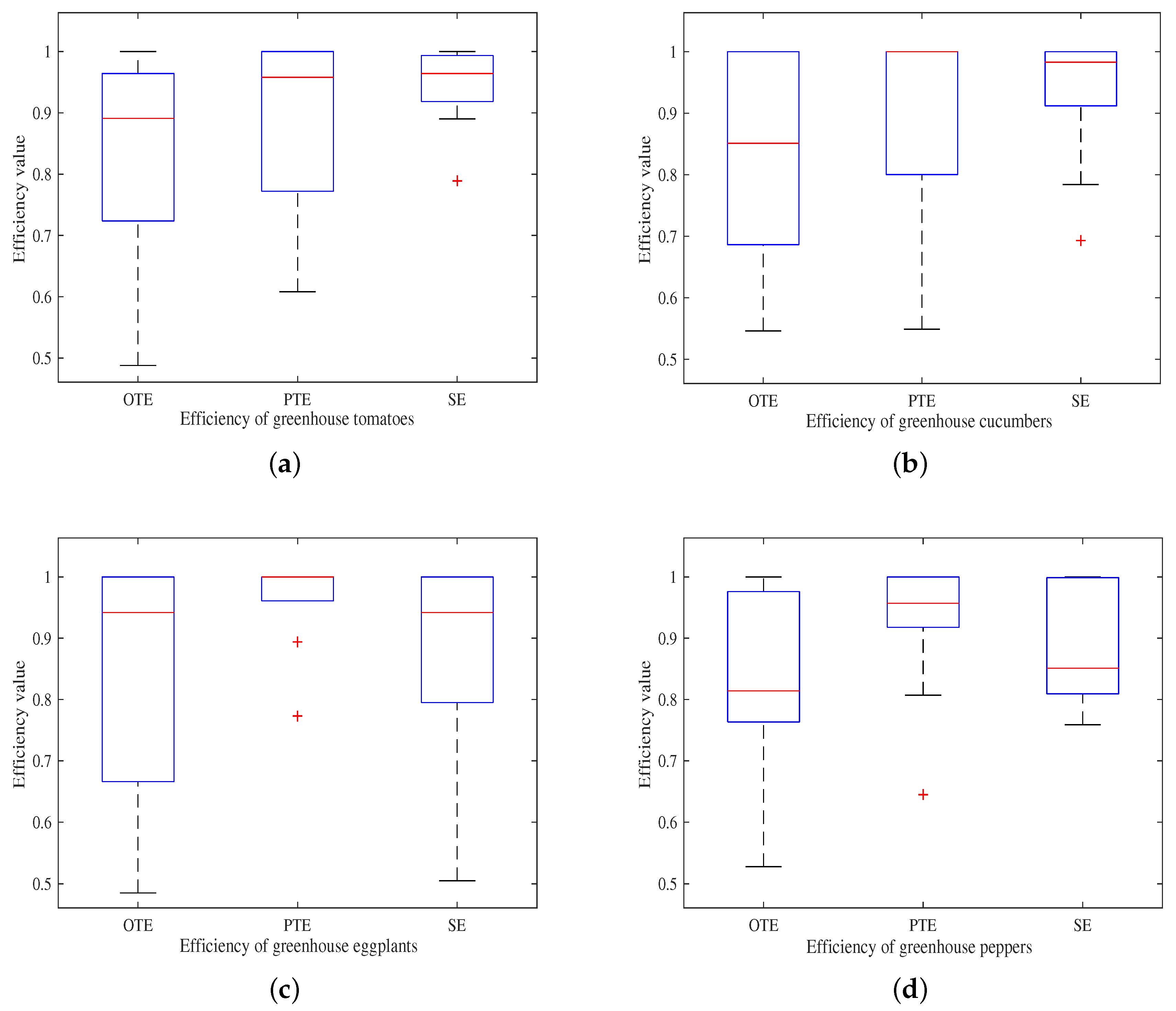
3.1. Comparative Analysis of Vegetable Efficiency in Greenhouses

Based on DEA model under BCC assumption, the production efficiency of greenhouse vegetables is calculated. The results of the DEA model represent the relative efficiency, and the results will change with different number of variables. In order to study the input–output efficiency of greenhouse vegetable planting provinces in China, four greenhouse vegetables were selected: greenhouse tomatoes, greenhouse cucumbers, greenhouse eggplants, and greenhouse peppers. According to the input–output data, DEAP2. 1 software was run to analyze the overall technical efficiency, pure technical efficiency, and scale efficiency of the four greenhouse vegetables. The relative production efficiency of greenhouse vegetables in each province can be judged by these efficiency values. Taking the production efficiency of greenhouse tomatoes as an example, the DEA model under BCC assumption was adopted. The results are shown in Figure 1 and Table 2. OTE represents the overall technical efficiency, PTE represents the pure technical efficiency, and SE represents the scale efficiency.
For greenhouse tomato cultivation in vegetable industry, the results are shown in Table 2 and Figure 1a. The average OTE, PTE, and SE of 21 provinces are 0.831, 0.872, and 0.950, respectively. Through the decomposition and comparison of efficiency, we can find that four provinces are effective, which are Tianjin, Heilongjiang, Hubei, and Xinjiang, respectively. However, Shandong Province has the lowest efficiency, which is only 0.488, followed by Inner Mongolia and Liaoning, with 0.603 and 0.628, respectively.
For the greenhouse cucumber cultivation in the vegetable industry, the results are shown in Figure 1b. The average OTE, PTE, and SE of 21 provinces are 0.821, 0.875, and 0.942, respectively. Through the decomposition and comparison of efficiency, we can find that seven provinces are effective, which are Beijing, Tianjin, Heilongjiang, Zhejiang, Hubei, Sichuan, and Xinjiang. However, Shanxi Province has the lowest efficiency, which is only 0.546, followed by Qinghai and Inner Mongolia, with 0.557 and 0.564, respectively. The difference between the maximum value and the minimum value is 0.454.
For greenhouse eggplant cultivation in vegetable industry, the results are shown in Figure 1c. The average OTE, PTE, and SE of 10 provinces are 0.837, 0.963, and 0.866, respectively. Through the decomposition and comparison of efficiency, we can find that four provinces are effective, which are Beijing, Tianjin, Liaoning, and Sichuan, respectively. However, Zhejiang Province has the lowest efficiency, which is only 0.458, followed by Shanxi Province and Shanghai, with 0.615 and 0.666, respectively.
For greenhouse pepper cultivation, the results are shown in Figure 1d. The average OTE, PTE, and SE of 11 provinces are 0.828, 0.928, and 0.888, respectively. Through the decomposition and comparison of efficiency, we can find that three provinces are effective, which are Beijing, Tianjin, and Sichuan. However, Gansu Province has the lowest efficiency, which is only 0.528, followed by Zhejiang Province with 0.634. The PTE is 0.645, and the SE is 0.786 in Gansu Province. The PTE is 0.807, and the SE is 0.786 in Zhejiang Province.
From the empirical results above, we can see that the OTE of greenhouse vegetables in different provinces is quite different. Only a few provinces are effective, most of them are in the state of increasing returns to scale or decreasing returns to scale. From the perspective of the PTE, vegetable greenhouses failed to make use of current technologies to maximize output under fixed input conditions in most provinces.

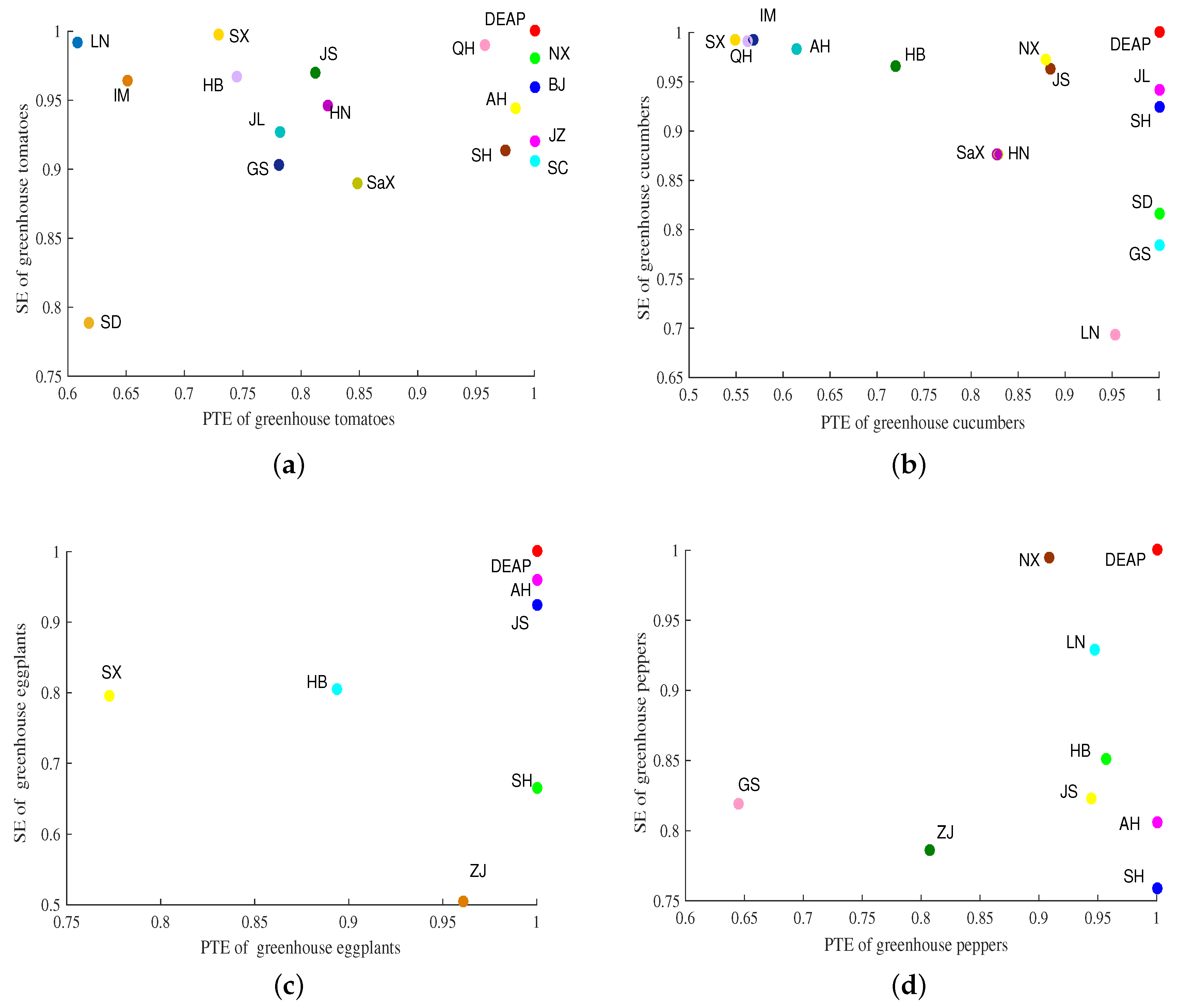
3.2. Comparison and Analysis of the Efficiency of Greenhouse Vegetables at Provincial Level

Based on the overall analysis of the efficiency of the four greenhouse vegetables, we can find that greenhouse vegetable efficiencies in many provinces of China are low. In Figure 2, we analyze the PTE and the SE of the four greenhouse vegetables. Based on the analysis of the PTE and the SE, this paper explores whether the PTE or the SE leads to the inefficiency of greenhouse vegetables.
By breaking down and comparing the efficiency of greenhouse tomatoes as shown in Figure 2a, we can find that four provinces are effective, which are Tianjin, Heilongjiang, Hubei, and Xinjiang, respectively. Among the other 17 provinces without DEA efficiency, the PTE of 11 provinces is lower than the SE. In other words, the loss of PTE may lead to inefficiency in most provinces. This indicates that the main obstacle to improving the efficiency of greenhouse tomato production in most parts of China is the difficulty in improving the PTE of greenhouse tomatoes.
By decomposing and comparing the efficiency of greenhouse cucumbers as shown in Figure 2b, it can be found that seven provinces are effective, namely Beijing, Tianjin, Heilongjiang, Zhejiang, Hubei, Sichuan, and Xinjiang, respectively. The difference between the maximum and minimum values is 0.454. Among the other 14 provinces without DEA efficiency, the PTE of nine provinces is lower than the SE. In other words, the loss of PTE may lead to inefficiency in most provinces. This shows that the difficulty of improving the PTE is the main obstacle to improve the efficiency of greenhouse cucumber production in most parts of China.
By breaking down and comparing the efficiency of greenhouse eggplants as shown in Figure 2c, we can find that four provinces are effective, namely Beijing, Tianjin, Liaoning, and Sichuan, respectively. Among the other six provinces without DEA efficiency, the SE of five provinces is lower than the PTE. In other words, the loss of SE may lead to inefficiency in most provinces. This indicates that the difficulty of increasing the SE is a major obstacle to improving the efficiency of greenhouse eggplant production in China.
By breaking down and comparing the efficiency of greenhouse peppers as shown in Figure 2d, we can find that three provinces are effective, namely Beijing, Tianjin, and Sichuan, respectively. Among the other eight provinces without DEA efficiency, the SE of six provinces is lower than the PTE. In other words, the loss of SE may lead to inefficiency in most provinces. This shows that the difficulty of improving the SE is the main obstacle to improve the production efficiency of greenhouse peppers in China.

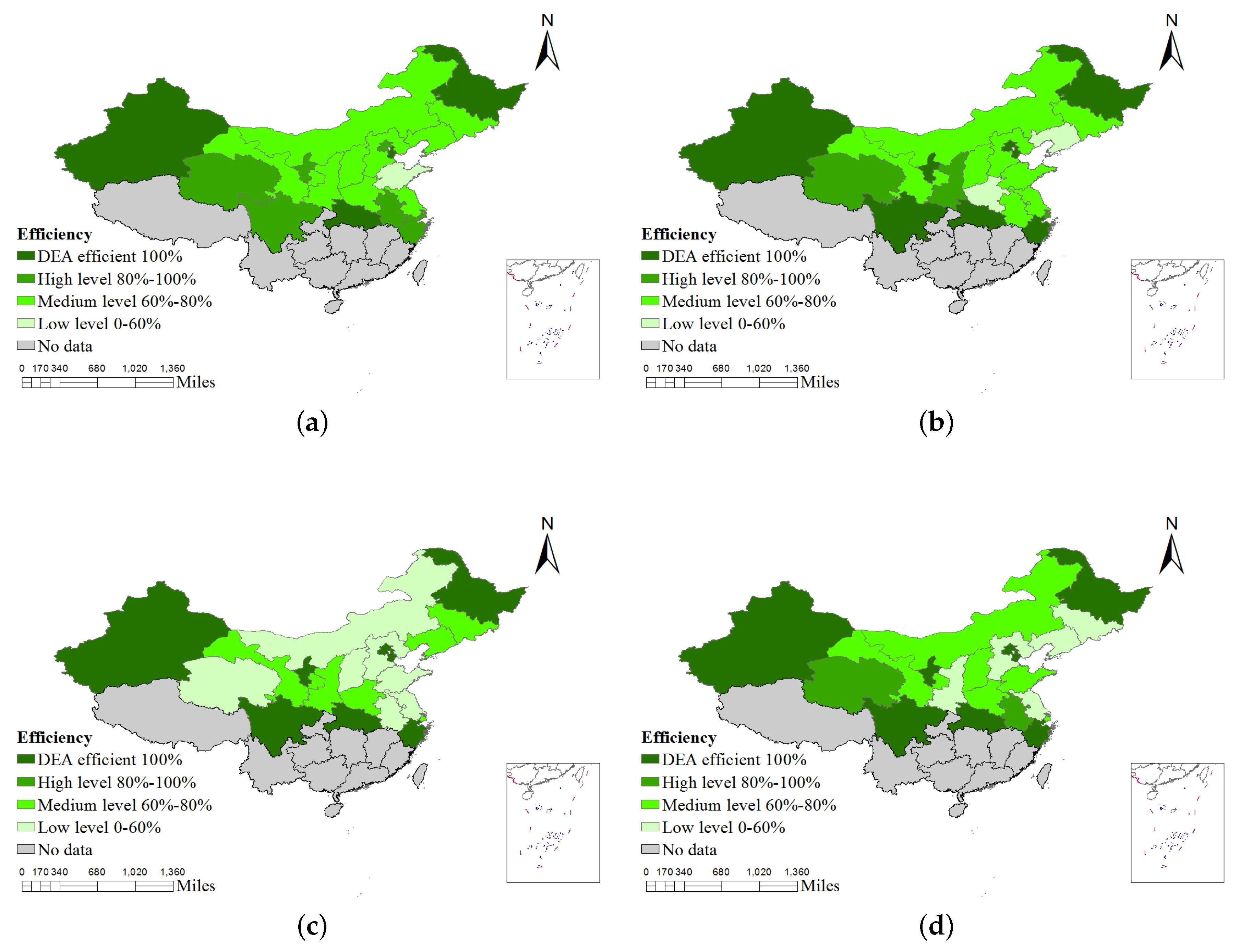
3.3. Spatial Distribution Analysis of Efficiency

In order to examine the spatial distribution of vegetable production efficiency in greenhouse, we use GIS 10.6 software to analyze the spatial distribution of vegetable production efficiency in greenhouse. In Figure 3, the distribution of greenhouse vegetable efficiency in different provinces is studied by taking greenhouse tomatoes as an example. We divide the comprehensive technical efficiency, the fertilizer efficiency, the farm fertilizer efficiency, and the pesticide efficiency into four categories. We use different colors to represent different levels. An efficiency value of 100% is classified as DEA efficiency. An efficiency value between 80% and 100% is classified as high level. An efficiency value between 60% and 80% is classified as medium level. An efficiency value between 0% and 60% is classified as low level. The gray areas in Figure 3 are with no data, most of which are located in the south of the Yangtze river. This is because there is plenty of sunshine and rain in the south of the Yangtze River. Most regions and provinces are mainly traditional uncovered farmland, with less vegetables planted in greenhouses.
Figure 3a shows the distribution of the comprehensive efficiency of greenhouse tomatoes in various provinces of China. On the whole, the OTE in most areas of China is not high. Tianjin, Heilongjiang, Xinjiang, and Hubei are in DEA efficient. Beijing, Shanghai, Zhejiang, Anhui, Sichuan, Qinghai, and Ningxia are high level of efficiency. Hebei, Shanxi, Inner Mongolia, Liaoning, Jilin, Jiangsu, Henan, Shaanxi, and Gansu are medium-level efficiency. Shandong Province has the lowest comprehensive efficiency, which is low-level efficiency.
Figure 3b shows the distribution of the efficiency of fertilizer in various provinces of China. It can be seen that most areas are in the medium level of fertilizer use efficiency, which can be improved a lot. Beijing, Tianjin, Heilongjiang, Zhejiang, Hubei, Sichuan, Ningxia, and Xinjiang are DEA efficient. Shanghai, Shaanxi, and Qinghai are of a high level of efficiency. Hebei, Shanxi, Inner Mongolia, Jilin, Jiangsu, Anhui, Shandong, and Gansu are medium-level efficiency. Liaoning and Henan are low-level efficiency. The utilization efficiency of chemical fertilizer in Henan and Liaoning provinces is less than 60%. In Henan Province, the use efficiency of fertilizer is low mainly because of the excessive use and intensity of fertilizer and the lack of use of farmyard manure [39]. In order to pursue a high yield, most provinces may use large amounts of elemental fertilizers excessively and frequently, resulting in low fertilizer use efficiency. If farmers use chemical fertilizer unreasonably, it will not only waste resources, but also cause environmental pollution [40].
Figure 3c shows the distribution of the use efficiency of farmyard manure in various provinces of China. Beijing, Tianjin, Heilongjiang, Zhejiang, Hubei, Sichuan, Ningxia, and Xinjiang are DEA efficient. Liaoning, Jilin, Shanghai, Henan, Shaanxi, and Gansu are medium-level efficiency. Hebei, Shanxi, Inner Mongolia, Jiangsu, Anhui, Shandong, and Qinghai are low-level efficiency. The efficiency of farm manure use in 13 provinces of China is less than 80%. This shows that the efficiency of farm manure use is low in most provinces of China, and there are big problems in the use of farm manure. The effective use of farmyard manure is conducive to reducing environmental pollution and reducing the damage of fertilizer to land [41]. Therefore, it is important to improve the utilization efficiency of farmyard manure for the cultivation of greenhouse vegetables in China.
Figure 3d shows the distribution of pesticide use efficiency in various provinces of China. Beijing, Tianjin, Heilongjiang, Zhejiang, Hubei, Sichuan, Ningxia, and Xinjiang are DEA efficient. Anhui and Qinghai are a high level of efficiency. Shanxi, Inner Mongolia, Shanghai, Shandong, Henan, and Gansu are medium-level efficiency. Hebei, Liaoning, Jilin, Jiangsu, and Shaanxi are low-level efficiency. As can be seen from the Figure 3d, the utilization efficiency of pesticides is less than 60% in most areas mainly along the east coast of China, such as Liaoning, Hebei, and Jiangsu. Although these areas are economically developed, the use of pesticides is not very efficient. Due to its proximity to the ocean and their humid climate, it is easy to breed a large number of pests. Farmers often use a lot of pesticides to control pests. This can easily lead to inefficient use of pesticides [42]. In addition, the utilization efficiency of pesticide in greenhouse tomatoes in Shaanxi Province is not high. The main reason for the low utilization rate of pesticide in Shaanxi Province may be the backward application equipment [5].

3.4. Analysis and Adjustment of Inefficient Provinces

The DEA method can not only explore the reasons why the decision-making unit is ineffective, but also give corresponding improvement methods. DEAP2.1 software is used to process the input–output data of greenhouse vegetable planting in main provinces of China in 2016, and we find that there is redundancy in greenhouse vegetable planting. This study mainly lists four kinds of greenhouse vegetables with redundancy in inputs. Table 3 shows the adjustment of greenhouse tomato planting provinces with redundancy.
According to the new situation of accelerated economic and social development in China, the whole country is divided into four major economic regions: the eastern region, the northeast region, the central region, and the western region. Similarly, according to the geographical location of greenhouse vegetable growing provinces, we divide the efficiency adjustment analysis of greenhouse vegetables into four regions: the eastern region, the northeast region, the central region, and the western region.

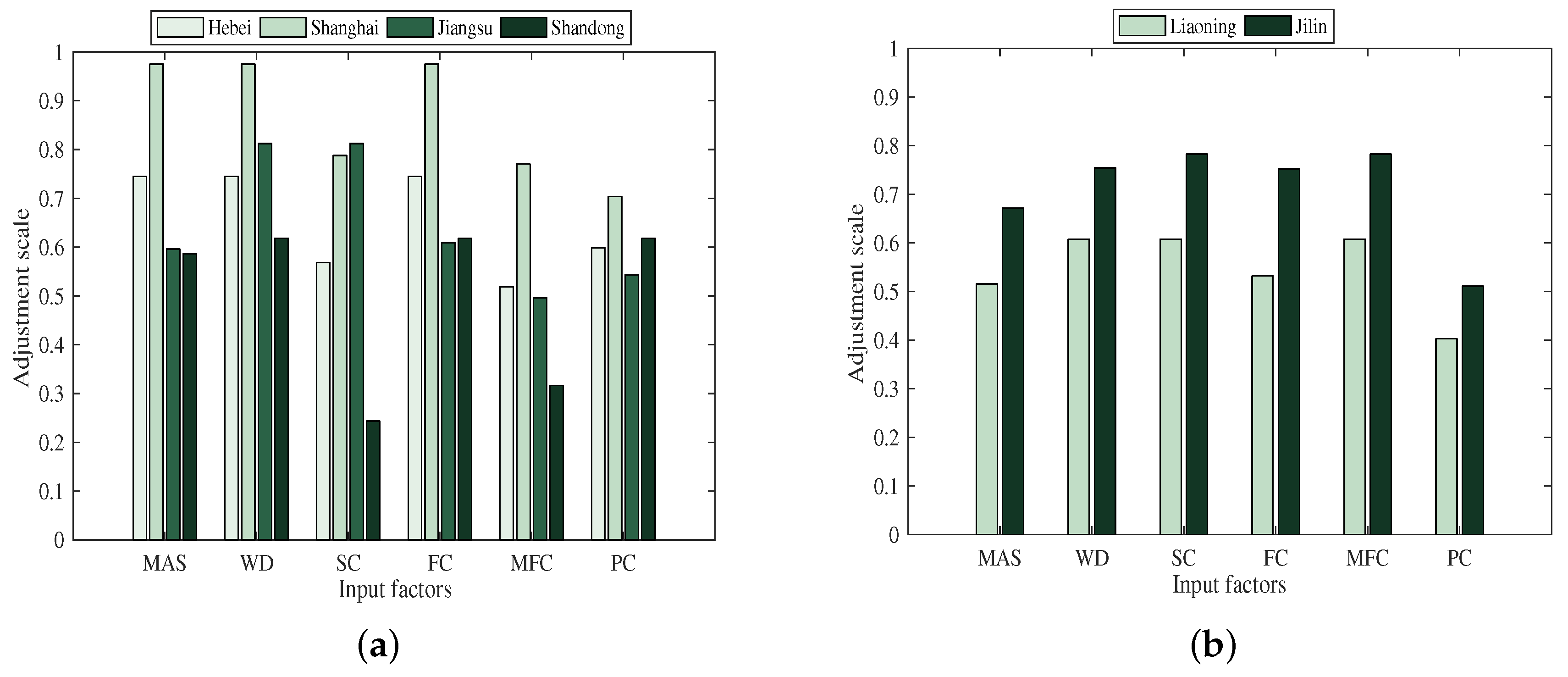
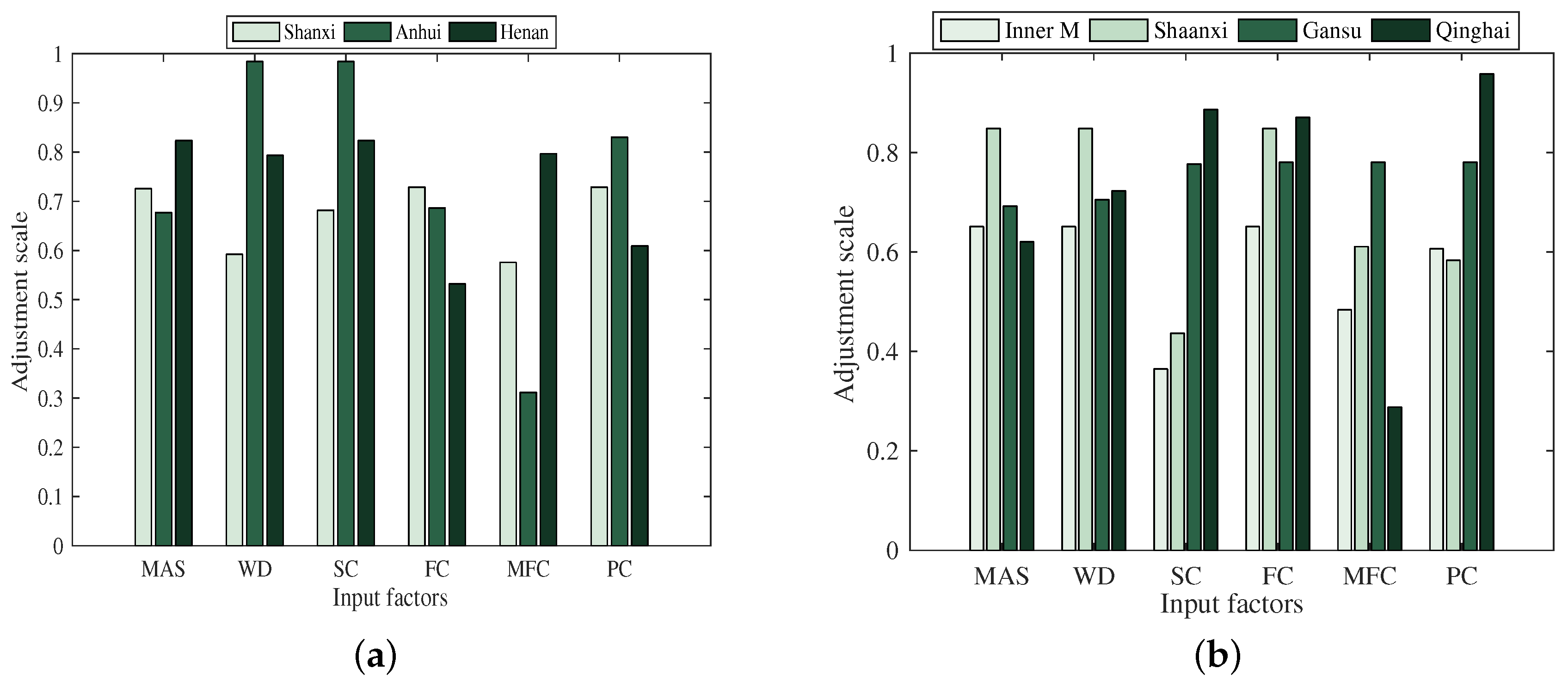
3.4.1. Analysis on the Adjustment of Efficiency Input in Eastern China

In Table 3, the production efficiency of greenhouse tomatoes in Hebei, Shanghai, Jiangsu, and Shandong is not effective in eastern China. The adjustment range is shown in Figure 4a. In Hebei Province, the adjustment ranges of six input factors of greenhouse tomatoes are 74.50%, 74.50%, 56.84%, 74.50%, 51.87%, and 59.87%, respectively, including material and service cost, number of working days, seed cost, fertilizer cost, farmyard manure cost, and pesticide cost. The adjustment ranges of six input factors of greenhouse tomatoes in Shanghai are 97.49%, 97.49%, 78.79%, 97.49%, 77.02%, and 70.36%, respectively. The adjustment ranges of six input factors of greenhouse tomatoes in Jiangsu Province are 59.61%, 81.24%, 81.24%, 60.90%, 49.62%, and 54.27%, respectively. The adjustment ranges of six input factors of greenhouse tomatoes in Shandong Province are 58.65%, 61.81%, 24.34%, 61.81%, 31.64%, and 61.81%, respectively.
In summary, there exist some problems of excessive investment in Hebei, Shanghai, and Shandong, resulting in a waste of energy and environmental pollution. In the eastern region, the excessive input of fertilizers in Jiangsu Province is 39.1%, while the excessive input of pesticides is 45.73%. The excessive input of pesticides in Hebei Province is 40.13%. The excessive input of fertilizers in Shandong Province is 38.19%, while the excessive input of pesticides is 38.19%.

3.4.2. Analysis on the Adjustment of Efficiency Input in Northeast China

In Table 3, the production efficiency of greenhouse tomatoes in Liaoning Province and Jilin Province is not effective in northeast China. The adjustment range is shown in Figure 4b. The adjustment ranges of six input factors of greenhouse tomatoes in Liaoning Province are 51.56%, 60.76%, 60.76%, 53.22%, 60.76%, and 40.28%, respectively, including material and service cost, number of working days, seed cost, fertilizer cost, farmyard manure cost, and pesticide cost. The adjustment ranges of six input factors of greenhouse tomatoes in Jilin Province are 67.16%, 75.43%, 78.25%, 75.21%, 78.25%, and 51.08%, respectively.
In short, there exist some problems of excessive investment in Liaoning and Jilin, resulting in the waste of resources and environmental pollution. The excessive input of fertilizers in Liaoning Province is 46.78%, while the excessive input of pesticides is 59.72%. The excessive input of pesticides in Jilin Province is 48.92%, while the excessive input of fertilizers is 24.79%.

3.4.3. Analysis on the Adjustment of Efficiency Input in Central China

In Table 3, the production efficiency of greenhouse tomatoes in Shanxi, Anhui and Henan is not effective in central China. The adjustment range is shown in Figure 5a. The adjustment ranges of six input factors of greenhouse tomatoes in Shanxi Province are 72.57%, 59.24%, 68.16%, 72.89%, 57.58%, and 72.89%, respectively, including material and service cost, number of working days, seed cost, fertilizer cost, farmyard manure cost, and pesticide cost. The adjustment ranges of six input factors of greenhouse tomatoes in Anhui Province are 67.70%, 98.42%, 98.42%, 68.65%, 31.15%, and 83.03%, respectively. In Henan Province, the adjustment ranges of six input factors of greenhouse tomatoes are 82.34%, 79.34%, 82.34%, 53.23%, 79.66%, and 60.91%, respectively.
To sum up, there exist some problems of excessive investment in Henan Province, Anhui Province, and Shanxi Province, resulting in the waste of resources and energy and environmental pollution. In the central region, the excessive input of fertilizers in Henan Province is 46.77%, and the excessive input of pesticides is 39.09%. The excessive input of fertilizers in Anhui Province is 31.35%. The excessive input of fertilizers in Shanxi Province is 27.11%, while the excessive input of pesticides is 27.11%.

3.4.4. Analysis on the Adjustment of Efficiency Input in Western China

In Table 3, the production efficiency of greenhouse tomatoes in Inner Mongolia, Shaanxi, Gansu and Qinghai is not effective in western China. The adjustment range is shown in Figure 5b. The adjustment ranges of six input factors of greenhouse tomatoes in Inner Mongolia are 65.11%, 65.11%, 36.47%, 65.11%, 48.38%, and 60.68%, respectively, including material and service cost, number of working days, seed cost, fertilizer cost, farmyard manure cost, and pesticide cost. The adjustment ranges of six input factors of greenhouse tomatoes in Shaanxi Province are 84.85%, 84.85%, 43.66%, 84.85%, 61.10%, and 58.36%, respectively. The adjustment ranges of six input factors of greenhouse tomatoes in Gansu Province are 69.24%, 70.53%, 77.70%, 78.09%, 78.09%, and 78.09%, respectively. The adjustment ranges of six input factors of greenhouse tomatoes in Qinghai Province are 62.05%, 72.32%, 88.69%, 87.12%, 28.83%, and 95.84%, respectively.
In general, there exist some problems of excessive investment in Inner Mongolia, Shaanxi, Qinghai, and Gansu, resulting in waste of energy and environmental pollution. In the western region, the excessive input of pesticides in Shaanxi Province is 41.64%. The excessive input of fertilizers in Inner Mongolia is 39.32%, while the excessive input of pesticides is 34.89%.

4. Conclusions and Policy Implication

This paper uses a DEA model to analyze the overall technical efficiency (OTE), pure technical efficiency (PTE), and scale efficiency (SE) of greenhouse tomatoes, greenhouse cucumbers, greenhouse eggplants, and greenhouse peppers from the perspective of greenhouse vegetable production efficiency. According to different efficiency values of greenhouse vegetables, we put forward some suggestions to adjust the different production efficiency. The main conclusions are as follows:
  • In the production of greenhouse tomatoes and cucumbers in China, the loss of PTE may lead to inefficiency in most provinces. For greenhouse tomatoes, among the 17 inefficient provinces, the PTE of 11 provinces is lower than the SE. For greenhouse cucumbers, among the 14 inefficient provinces, the PTE of 9 provinces is lower than the SE. The results show that the government should pay more attention to the improvement of the PTE of greenhouse tomatoes and cucumbers.
  • In the production of greenhouse eggplants and peppers in China, the loss of SE may lead to inefficiency in most provinces. For greenhouse eggplants, among the six inefficient provinces, the SE of five provinces is lower than the PTE. For greenhouse peppers, among the eight inefficient provinces, the SE of six provinces is lower than the PTE. The results show that the government should pay more attention to improving the SE of greenhouse eggplants and peppers.
  • From the perspective of input factors, fertilizers, farm manure and pesticides are inefficient in most parts of China. In particular, the overall use efficiency of farmyard manure is low, and chemical fertilizers and pesticides are seriously wasted. These results indicate that the government should pay more attention to the use of chemical fertilizers, farm manure, and pesticides to improve the use efficiency in the future. On the one hand, it helps to reduce the waste of resource. On the other hand, it is conducive to the development of green and sustainable agriculture.
Based on the above analysis, we put forward some suggestions for the different characteristics of the efficiency of greenhouse vegetables in different provinces. The suggestions are as follows:
  • For provinces with DEA efficiency, such as Tianjin, Heilongjiang, and Hubei, on the basis of maintaining the existing production advantages, the supply and demand of greenhouse vegetable production should be balanced. For the provinces with high level of efficiency, such as Beijing, Sichuan, Shanghai, and Ningxia, the government should maintain the existing scale advantage in promoting vegetable production development at first. Thus, the government should focus on the introduction and application of advanced field technology and management mode to achieve higher utilization rate of input factors in greenhouse vegetable production.
  • For the provinces with low level of efficiency, such as Shandong, Inner Mongolia, Shanxi, and Hebei, it is important to improve the PTE and find the appropriate scale suitable for the local. First, the government should increase support to these provinces and guide farmers to use chemical fertilizers and pesticides rationally. Second, the government should encourage and support the use of farm manure to reduce the use of chemical fertilizers.
In the next study, we plan to study the change of greenhouse vegetable production efficiency from the perspective of time series and space in China. It is planned to use the DEA model and Tobit model to explore the influencing factors of greenhouse vegetable production efficiency, in order to make a contribution to the development of green and sustainable agriculture.

Author Contributions

All authors contributed to this study. J.R. and Y.L. formulated the study design. J.R., Y.S., Y.L., and Y.W. conceived and designed the research methodology. X.J., J.R., and Y.L. collected and analyzed the data. J.R. and Y.L. finalized the paper.

Funding

This work was supported in part by the National Natural Science Foundation of China under Grants 71703122, 71973106, and 71531002, the China Ministry of Education Social Sciences and Humanities Research Youth Fund Project under Grant 16YJC630102, the Science and Technology Plan Projects of Yangling Demonstration Zone under Grant 2016RKX-04, the Fundamental Research Funds for the Central Universities under Grant 2018RWSK02, the Key Research and Development Program of Shaanxi under Grant 2019ZDLNY07-02-01, and the National College Students’ Innovation and Entrepreneurship Training Program under Grant 201910712075.

Acknowledgments

We thank the National Nature Science Foundation of China, China Ministry of Education Social Sciences and Humanities Research Youth Fund Project, Natural Science Basic Research Project in Shaanxi Province, Science and Technology Plan Projects of Yangling Demonstration Zone, Fundamental Research Funds for the Central Universities, Key Research and Development Program of Shaanxi and National College Students’ Innovation and Entrepreneurship Training Program for funding the research.

Conflicts of Interest

The authors declare no conflict of interest.

References

  1. Xu, L.; Wang, Y.; Shah, S.A.A.; Zameer, H.; Solangi, Y.A.; Walasai, G.D.; Siyal, Z.A. Economic viability and environmental efficiency analysis of hydrogen production processes for the decarbonization of energy systems. Processes 2019, 7, 494. [Google Scholar] [CrossRef]
  2. Hafeez, G.; Islam, N.; Ali, A.; Ahmad, S.; Usman, M.; Alimgeer, K.S. A modular framework for optimal load scheduling under price-based demand response scheme in smart grid. Processes 2019, 7, 499. [Google Scholar] [CrossRef]
  3. Ruan, J.; Wang, Y.; Chan, F.T.S.; Hu, X.; Zhao, M.; Zhu, F.; Shi, B.; Shi, Y.; Lin, F. A life cycle framework of green IoT-based agriculture and its finance, operation, and management issues. IEEE Commun. Mag. 2019, 57, 90–96. [Google Scholar] [CrossRef]
  4. Ruan, J.; Jiang, H.; Li, X.; Shi, Y.; Chan, F.T.; Rao, W. A granular GA-SVM predictor for big data in agricultural cyber-physical systems. IEEE Trans. Ind. Inf. 2019, 57, 90–96. [Google Scholar] [CrossRef]
  5. Clark, M.; Tilman, D. Comparative analysis of environmental impacts of agricultural production systems, agricultural input efficiency, and food choice. Environ. Res. Lett. 2017, 12, 1–12. [Google Scholar] [CrossRef]
  6. Geng, Q.; Ren, Q.; Nolan, R.H.; Wu, P.; Yu, Q. Assessing China’s agricultural water use efficiency in a green-blue water perspective: A study based on data envelopment analysis. Ecol. Indic. 2019, 96, 329–335. [Google Scholar] [CrossRef]
  7. Liu, S.; Zhang, S.; He, X.; Li, J. Efficiency change in North-East China agricultural sector: A DEA approach. Agric. Econ. 2015, 61, 522–532. [Google Scholar] [CrossRef]
  8. Pang, J.; Chen, X.; Zhang, Z.; Li, H. Measuring eco-efficiency of agriculture in China. Sustainability 2016, 8, 398. [Google Scholar] [CrossRef]
  9. Baráth, L.; Ferto, I. Productivity and convergence in European agriculture. J. Agric. Econ. 2017, 68, 228–248. [Google Scholar] [CrossRef]
  10. Toma, E.; Dobre, C.; Dona, I.; Cofas, E. DEA applicability in assessment of agriculture efficiency on areas with similar geographically patterns. Agric. Agric. Sci. Procedia 2015, 6, 704–711. [Google Scholar] [CrossRef]
  11. Raheli, H.; Rezaei, R.M.; Jadidi, M.R.; Mobtaker, H.G. A two-stage DEA model to evaluate sustainability and energy efficiency of tomato production. Inf. Process. Agric. 2017, 4, 342–350. [Google Scholar] [CrossRef]
  12. Cardozo, N.P.; de Oliveira Bordonal, R.; La Scala, N., Jr. Sustainable intensification of sugarcane production under irrigation systems, considering climate interactions and agricultural efficiency. J. Clean. Prod. 2018, 204, 861–871. [Google Scholar] [CrossRef]
  13. Grados, D.; Schrevens, E. Multidimensional analysis of environmental impacts from potato agricultural production in the Peruvian Central Andes. Sci. Total Environ. 2019, 663, 927–934. [Google Scholar] [CrossRef] [PubMed]
  14. Singbo, A.G.; Lansink, A.O.; Emvalomatis, G. Estimating shadow prices and efficiency analysis of productive inputs and pesticide use of vegetable production. Eur. J. Oper. Res. 2015, 245, 265–272. [Google Scholar] [CrossRef]
  15. Rajendran, S.; Afari-Sefa, V.; Karanja, D.K.; Musebe, R.; Romney, D.; Makaranga, M.A.; Samali, S.; Kessy, R.F. Technical efficiency of traditional African vegetable production: A case study of smallholders in Tanzania. J. Dev. Agric. Econ. 2015, 7, 92–99. [Google Scholar]
  16. Ajekiigbe, N.; Ayanwale, A.; Oyedele, D.; Adebooye, O. Technical efficiency in production of underutilized indigenous vegetables. Int. J. Veg. Sci. 2018, 24, 193–201. [Google Scholar] [CrossRef]
  17. Duan, N.; Guo, J.P.; Xie, B.C. Is there a difference between the energy and CO2 emission performance for China’s thermal power industry? A bootstrapped directional distance function approach. Appl. Energy 2016, 162, 1552–1563. [Google Scholar] [CrossRef]
  18. Riccardi, R.; Oggioni, G.; Toninelli, R. Efficiency analysis of world cement industry in presence of undesirable output: Application of data envelopment analysis and directional distance function. Energy Policy 2012, 44, 140–152. [Google Scholar] [CrossRef]
  19. Choi, Y.; Zhang, N.; Zhou, P. Efficiency and abatement costs of energy-related CO2 emissions in China: A slacks-based efficiency measure. Appl. Energy 2012, 98, 198–208. [Google Scholar] [CrossRef]
  20. Lee, T.; Yeo, G.T.; Thai, V.V. Environmental efficiency analysis of port cities: Slacks-based measure data envelopment analysis approach. Transp. Policy 2014, 33, 82–88. [Google Scholar] [CrossRef]
  21. Li, L.B.; Hu, J.L. Ecological total-factor energy efficiency of regions in China. Energy Policy 2012, 46, 216–224. [Google Scholar] [CrossRef]
  22. Zhang, N.; Zhou, P.; Kung, C.C. Total-factor carbon emission performance of the Chinese transportation industry: A bootstrapped non-radial Malmquist index analysis. Renew. Sustain. Energy Rev. 2015, 41, 584–593. [Google Scholar] [CrossRef]
  23. Zhou, G.; Chung, W.; Zhang, Y. Measuring energy efficiency performance of China’s transport sector: A data envelopment analysis approach. Expert Syst. Appl. 2014, 41, 709–722. [Google Scholar] [CrossRef]
  24. Emrouznejad, A.; Yang, G.L. CO2 emissions reduction of Chinese light manufacturing industries: A novel RAM-based global Malmquist–Luenberger productivity index. Energy Policy 2016, 96, 397–410. [Google Scholar] [CrossRef]
  25. Wu, J.; Lv, L.; Sun, J.; Ji, X. A comprehensive analysis of China’s regional energy saving and emission reduction efficiency: From production and treatment perspectives. Energy Policy 2015, 84, 166–176. [Google Scholar] [CrossRef]
  26. Fei, R.; Lin, B. Energy efficiency and production technology heterogeneity in China’s agricultural sector: A meta-frontier approach. Technol. Forecast. Soc. Chang. 2016, 109, 25–34. [Google Scholar] [CrossRef]
  27. Fei, R.; Lin, B. The integrated efficiency of inputs–outputs and energy–CO2 emissions performance of China’s agricultural sector. Renew. Sustain. Energy Rev. 2017, 75, 668–676. [Google Scholar] [CrossRef]
  28. Li, N.; Jiang, Y.; Mu, H.; Yu, Z. Efficiency evaluation and improvement potential for the Chinese agricultural sector at the provincial level based on data envelopment analysis (DEA). Energy 2018, 164, 1145–1160. [Google Scholar] [CrossRef]
  29. Le, T.L.; Lee, P.P.; Peng, K.C.; Chung, R.H. Evaluation of total factor productivity and environmental efficiency of agriculture in nine East Asian countries. Agric. Econ. 2019, 65, 249–258. [Google Scholar]
  30. Wang, F.; Yu, C.; Xiong, L.; Chang, Y. How can agricultural water use efficiency be promoted in China? A spatial-temporal analysis. Resour. Conserv. Recycl. 2019, 145, 411–418. [Google Scholar] [CrossRef]
  31. Lampe, H.W.; Hilgers, D. Trajectories of efficiency measurement: A bibliometric analysis of DEA and SFA. Eur. J. Oper. Res. 2015, 240, 1–21. [Google Scholar] [CrossRef]
  32. Ahmad, Z.; Jun, M. Agricultural Production Structure Adjustment Scheme Evaluation and Selection Based on DEA Model for Punjab (Pakistan). J. Northeast Agric. Univ. (Engl. Ed.) 2015, 22, 87–91. [Google Scholar] [CrossRef]
  33. e Souza, G.D.S.; Gomes, E.G. Management of agricultural research centers in Brazil: A DEA application using a dynamic GMM approach. Eur. J. Oper. Res. 2015, 240, 819–824. [Google Scholar] [CrossRef] [Green Version]
  34. Zhu, N.; Hougaard, J.L.; Ghiyasi, M. Ranking production units by their impact on structural efficiency. J. Oper. Res. Soc. 2019, 70, 783–792. [Google Scholar] [CrossRef]
  35. Rahman, M.T.; Nielsen, R.; Khan, M.A.; Asmild, M. Efficiency and production environmental heterogeneity in aquaculture: A meta-frontier DEA approach. Aquaculture 2019, 509, 140–148. [Google Scholar] [CrossRef]
  36. Charnes, A.; Cooper, W.W.; Rhodes, E. Measuring the efficiency of decision making units. Eur. J. Oper. Res. 1978, 2, 429–444. [Google Scholar] [CrossRef]
  37. Banker, R.D.; Charnes, A.; Cooper, W.W. Some models for estimating technical and scale inefficiencies in data envelopment analysis. Manag. Sci. 1984, 30, 1078–1092. [Google Scholar] [CrossRef]
  38. Fenyves, V.; Tarnóczi, T.; Zsidó, K. Financial performance evaluation of agricultural enterprises with DEA method. Procedia Econ. Financ. 2015, 32, 423–431. [Google Scholar] [CrossRef]
  39. Adesemoye, A.O.; Kloepper, J.W. Plant–microbes interactions in enhanced fertilizer-use efficiency. Appl. Microbiol. Biotechnol. 2009, 85, 1–12. [Google Scholar] [CrossRef]
  40. Tilman, D.; Cassman, K.G.; Matson, P.A.; Naylor, R.; Polasky, S. Agricultural sustainability and intensive production practices. Nature 2002, 418, 671–677. [Google Scholar] [CrossRef]
  41. Idrees, M.; Batool, S.; Hussain, Q.; Ullah, H.; Al-Wabel, M.I.; Ahmad, M.; Kong, J. High-efficiency remediation of cadmium (Cd2+) from aqueous solution using poultry manure–and farmyard manure–derived biochars. Sep. Sci. Technol. 2016, 51, 2307–2317. [Google Scholar] [CrossRef]
  42. Vymazal, J.; Březinová, T. The use of constructed wetlands for removal of pesticides from agricultural runoff and drainage: A review. Environ. Int. 2015, 75, 11–20. [Google Scholar] [CrossRef] [PubMed]
Figure 1. Boxplot of OTE, PTE, and SE of greenhouse tomatoes (a), greenhouse cucumbers (b), greenhouse eggplants (c) and greenhouse peppers (d).
Processes 07 00780 g001
Figure 2. Efficiency distribution map of greenhouse tomatoes (a), greenhouse cucumbers (b), greenhouse eggplants (c) and greenhouse peppers (d).
Processes 07 00780 g002
Figure 3. Spatial distribution map of OTE (a), fertilizer efficiency (b), farm manure efficiency, (c) and pesticide efficiency (d) of greenhouse tomato.
Processes 07 00780 g003
Figure 4. Analysis results: (a) the proportion of efficiency input adjustment in eastern China; (b) the proportion of efficiency input adjustment in north-east China.
Processes 07 00780 g004
Figure 5. Analysis results: (a) the proportion of efficiency input adjustment in central China; (b) the proportion of efficiency input adjustment in western China.
Processes 07 00780 g005
Table 1. Classification and description of variables.
Variable ClassificationVariable NamesDefinitionsUnits
OutputOVMPOutput value of main productKilogram
MSCMaterial and service costYuan
SCSeed costYuan
FCFertilizer costYuan
InputsFMCFarmyard manure costYuan
PCPesticide costYuan
WDWorking daysDay
SAcreage of greenhouse vegetablesm 2
OVOriginal value of an output or input variableKilogram or yuan or day
Constraint variableRMRadial adjustment of an input variableKilogram or yuan or day
SMSlack movement of an input variableKilogram or yuan or day
PVTarget value of an output or input variableKilogram or yuan or day
Table 2. The overall technical efficiency (OTE), pure technical efficiency (PTE), and scale efficiency (SE) of greenhouse tomatoes.
ProvinceOTEPTESESR
Beijing0.9591.0000.959 d r s
Tianjin1.0001.0001.000
Hebei0.7200.7450.967 i r s
Shanxi0.7280.7290.998 d r s
Inner M0.6280.6510.964 i r s
Liaoning0.6030.6080.992 i r s
Jilin0.7250.7820.927 i r s
Heilongjiang1.0001.0001.000
Shanghai0.8910.9750.914 i r s
Jiangsu0.7880.8120.970 i r s
Zhejiang0.9201.0000.920 i r s
Anhui0.9290.9840.944 i r s
Shandong0.4880.6180.789 i r s
Henan0.7790.8230.946 d r s
Hubei1.0001.0001.000
Sichuan0.9061.0000.906 d r s
Shaanxi0.7560.8480.890 i r s
Gansu0.7050.7810.903 d r s
Qinghai0.9490.9580.990 i r s
Ningxia0.9801.0000.980 i r s
Xinjiang1.0001.0001.000
Note: SR means returns to scale, i r s means increasing returns to scale, d r s means decreasing returns to scale, and − means no change in return on scale.
Table 3. Input redundancy of greenhouse tomato planting per 667 m 2 in China in 2016.
ProvincesItemOVMP/kgMSC/YuanWD/dSC/YuanFC/YuanFMC/YuanPC/Yuan
HebeiOV5385.833199.9661.4399.1476.45425.39258.27
RM0−816.13−15.66−101.788−121.516−108.493−65.87
SM000−70.4470−96.231−37.778
PV5385.832383.8345.74226.865354.934220.666154.621
ShanxiOV5494.793733.4183.39323.54342.74515.99180.6
RM0−1012.13−22.607−87.712−92.917−139.885−48.961
SM0−11.84−11.385−15.3040−78.9740
PV5494.792709.44449.398220.524249.823297.131131.639
Inner MOV5384.683704.1968.07636.82584.67433.84266.01
RM0−1292.45−23.751−222.197−204.001−151.374−92.815
SM000−182.3950−72.588−11.777
PV5384.682411.73644.319232.227380.669209.878161.418
LiaoningOV5148.085559.3771.11329.09591.24368.22408.8
RM0−2181.35−27.902−29.126−231.987−144.48−160.402
SM0−511.44600−44.5960−83.724
PV5148.082866.57743.208199.964314.657223.74164.674
JilinOV4484.962438.4468.55165.52333.46191.17255.3
RM0−530.439−14.912−36.006−72.538−41.586−55.536
SM355.543−270.354−1.930−10.1410−69.356
PV4840.5031637.64751.708129.514250.78149.584130.408
ShanghaiOV4651.632132.1948.79193.17298.41210.83206.49
RM0−53.546−1.225−4.851−7.494−5.295−5.186
SM283.25200−36.1190−43.15−56.025
PV4934.8822078.64447.565152.2290.916162.385145.279
JiangsuOV4715.232752.1366.11152.82347.68344.18221.79
RM0−516.325−12.403−28.67−65.228−64.571−41.61
SM146.542−595.32700−70.721−108.826−59.818
PV4861.7721640.47753.707124.15211.731170.783120.362
AnhuiOV4538.32412.2949.23140.46457.91369.43176.76
RM0−38.023−0.776−2.214−7.218−5.823−2.786
SM267.584−741.22600−136.351−248.527−27.214
PV4805.8841633.04148.454138.246314.341115.08146.76
ShandongOV4404.74148.1768.61769.7589.55492.77290.14
RM0−1584.34−26.205−293.978−225.172−188.208−110.816
SM520.407−131.0780−288.3680−148.6470
PV4925.1072432.74842.405187.354364.378155.915179.324
HenanOV5105.422664.365.01193.99406.89286.88204.75
RM0−470.577−11.482−34.263−71.866−50.67−36.164
SM00−1.9460−118.426−7.683−43.883
PV5105.422193.72351.582159.727216.598228.528124.704
ShaanxiOV4512.172244.6260.49314.83275.67293.67220.67
RM0−340.163−9.167−47.711−41.777−44.504−33.442
SM407.07600−129.6510−69.72−58.445
PV4919.2461904.45751.323137.468233.893179.446128.783
GansuOV5473.013259.0673.93295.34451.16278.32232.8
RM0−713.899−16.194−64.694−98.827−60.966−50.995
SM0−288.45−5.592−1.158000
PV5473.012256.7152.143229.487352.333217.354181.805
QinghaiOV5781.853955.870.16302.58344.481092.73138.07
RM0−164.427−2.916−12.577−14.319−45.42−5.739
SM0−1336.75−16.504−21.657−30.038−732.3280
PV5781.852454.62950.74268.346300.124314.982132.331

