Modeling Parallel Robot Kinematics for 3T2R and 3T3R Tasks Using Reciprocal Sets of Euler Angles


Institute of Mechatronic Systems, Leibniz University Hannover, 30167 Hannover, Germany
*
Author to whom correspondence should be addressed.
Robotics 2019, 8(3), 68; https://doi.org/10.3390/robotics8030068
Submission received: 27 June 2019
/
Revised: 31 July 2019
/
Accepted: 1 August 2019
/
Published: 6 August 2019
(This article belongs to the Special Issue Kinematics and Robot Design II, KaRD2019)
Abstract
:Industrial manipulators and parallel robots are often used for tasks, such as drilling or milling, that require three translational, but only two rotational degrees of freedom (“3T2R”). While kinematic models for specific mechanisms for these tasks exist, a general kinematic model for parallel robots is still missing. This paper presents the definition of the rotational component of kinematic constraints equations for parallel robots based on two reciprocal sets of Euler angles for the end-effector orientation and the orientation residual. The method allows completely removing the redundant coordinate in 3T2R tasks and to solve the inverse kinematics for general serial and parallel robots with the gradient descent algorithm. The functional redundancy of robots with full mobility is exploited using nullspace projection.
1. Introduction
Industrial tasks like welding, gluing, milling or drilling represent a major part of the applications of industrial robots, which generally have full mobility, i.e., the operational space of their end-effector has three translational and three rotational (“3T3R”) degrees of freedom (“DoF”). Parallel robots like the Stewart platform have especially been proposed for milling tasks regarding their high structural stiffness. The task space of the named applications can be defined by three translational DoF and only two rotations due to a symmetry around the tool axis (“3T2R”). This results in a functional or task redundancy, which is not exploited to full extend yet for parallel robots.
1.1. Inverse Kinematics and Resolution of Task Redundancy for Serial-Link Robots
Various general gradient-based methods exist to solve the inverse kinematics for serial robots; either by augmenting the joint space [1] or by reducing the task space [2,3,4,5]. The different approaches each define a residual vector and a gradient matrix considering the properties of 3T2R tasks, e.g., by adding a virtual joint axis [1], orthogonal decomposition of the task space [2], rotation of the residual into a task frame and removing the corresponding component [3], defining the tool axis by two points for constructing a nullspace [4] or by defining the absolute orientation and the orientation residual with two reciprocal sets of Euler angles [5]. The gradient matrices corresponding to the different residuals are used for an iterative Newton-Raphson algorithm [6,7] by exploiting the functional redundancy with a null space projection of additional performance criteria [6]. Without the definition of a proper gradient, a global optimization has to be performed outside of the inverse kinematics algorithm [8,9].
1.2. Overview of Parallel Robots Structures for 3T2R Tasks
Parallel robots in 3T2R tasks can be ordered in classes according to their kinematic structure into
- I
- mechanisms with full platform mobility (3T3R) that are redundantly controlled to five DoF,
- II
- mechanisms with 3T2R platform mobility enforced with a passive five-DoF constraining leg and five other legs with six DoF each,
- III
- mechanisms with 3T2R platform mobility resulting from the mobility of five actuated legs with five or six DoF each,
- IV
- mechanisms with 3T2R platform mobility and five legs with only five DoF each.
The classes I and II were introduced in [10], where class IV is analyzed regarding leg symmetry and singularities. Class III is mainly influenced by the systematic synthesis of [11] and several existing prototypes and is demarcated against class II by the absence of the passive constraining leg. Class IV can be seen as a subclass of III, but is differentiated in this paper due to its characteristics. Other classifications are provided e.g., by [12], where IV and II are termed “families”.
Examples for the first class are hexapods (6UPS) [13] or the Eclipse [14] machine tool (2PPRS-PPRS). (The joint structure of the parallel robots is denoted by the number of the legs and the order of universal (“U”), prismatic (“P”), spherical (“S”), helical (“H”) and revolute (“R”) joints in the leg chains. Different actuated legs are connected by hyphens (“-”), passive constraint legs are connected by a slash (“/”). Actuated joints are underlined.) Any other parallel robot with full mobility (see e.g., [11,15,16]) may be used as well.
The second class allows for more variety, since the six-DoF mechanism and the five-DoF constraining leg can manifest in different kinematic structures: The UPS structure is used for the six-DoF part of the mechanism by [17] with a focus on kinematic analysis of 5UPS/US, by [18] with a focus on kinetostatic modeling at the example of 5UPS/RUU (see Figure 1a), by [19] with focus on trajectory control of 5UPS/PRPU and by [20] for pose measurement with the passive leg of 5UPS/PRPU. Other possible general base structures are RUS at the 5RUS/US example in [17], PUS, which has been investigated for the control of a redundantly actuated 6PUS/UPU regarding the force control of the redundant leg with inverse dynamics compensation [21] or force optimization [22].
The most-straightforward member of the third class is the 4UPS-UPU of Figure 1b, which is investigated in [23] for a simulation and feasibility study together with a survey on possible architectures for a technical realization of this class. Other possible structures are the 4URS-URU, which is analyzed kinematically in [24] and the 4PSU-PU*U, which has a special parallelogram structure in one leg (termed “U*”) and is presented in [25]. A subclass of III consists of mechanisms [26,27,28], where the last joint axis of the legs is coaxial with the tool axis and is constructed as rotating ring. It contains the Metrom machine tool (4SPRR-SPR), depicted in Figure 1c, which is analyzed regarding inverse and forward kinematics in [26] or its variants, the redundant 4SPRR-PSPR from [28] or the hybrid 4URHU-URHR with an additional linear actuator at the platform [27]. A structural synthesis based on linear transformations and evolutionary morphology [11] led e.g., to the Isoglide5 mechanisms (3PRRRRR-2PRRRR), which are analyzed and optimized regarding the isotropy of the Jacobian in [29].
The simplest member of class IV, the 5UPU is shown in [30] with the help of screw theory to only have local mobility and no global mobility, since the twist systems of the leg chains have no intersection and the resulting twist system of the platform is empty. Members of class IV have been found by systematic structural synthesis with screw theory, which has been performed in [31] for symmetric 3T2R mechanisms. The resulting 5RPUR of Figure 1d and 5PRUR are analyzed in [10,32].
In a practical application with competing requirements on workspace, stiffness, costs and precision, each of the existing systems has its legitimization. Nevertheless, each of the classes has inherent disadvantages: In tasks like milling with high process forces and requirements on stiffness and precision, robots from class II with one constraining leg have the drawback that the passive leg takes the complete reaction wrench in the blocked rotational degree of freedom, which strongly affects the mechanisms stiffness in this direction [18]. The same is argued by [27] at the example of the Metrom machine tool, but can be extended to all the members of class III, where most leg chains have six DoF and usually only one leg chain has five DoF. This leg chain also has to take the reaction moments in the blocked DoF which affects the overall stiffness. Therefore, members of the classes I and IV can be expected to reach a higher stiffness. Mechanisms of the class IV may further suffer from an increased sensitivity of manufacturing tolerances, which may cause a high pretension of the bearings or even reduce the DoF, since the five DoF of all leg chains have to coincide exactly to allow the platform to also have five DoF. Additionally, only members of class I provide redundancy which allows using the additional DoF for performance optimizations, e.g., to avoid singularities and to compensate the smaller workspace caused by the sixth leg.
Therefore, the remainder of the paper focuses on mechanisms of the first class to allow an optimization of their performance criteria using the degree of task redundancy.
1.3. Inverse Kinematics of Parallel Robots for 3T2R Tasks
The parallel robots with five DoF presented above have a kinematic structure which allows for an analytic model of the inverse kinematics. All references define the end-effector orientation with two consecutive elementary rotations, i.e., define two Euler angles to represent the tool axis orientation in minimal coordinates [10,13,19,20,21,22,26,28,32,33], which is called “partial pose” in [13]. The inverse kinematics problem (IKP) is first solved for the first chain, which is called “leading chain” in this paper. Due to the geometry of the leading chain, this solution can be found algebraically. Then the IKP is solved for the other “following” chains with the given orientation from the leading chain and standard methods. For robots of class II, the constraining leg is selected as the leading leg chain and for class III the 3T2R leg is selected.
To the best knowledge of the authors, only one reference [13] for the IKP of functionally redundant parallel robots of the class I is known. The reason presumably is that a solution of the 3T3R IKP for these robots is possible with standard methods, as used in [14] for the 3T3R Eclipse. It is always possible to transfer the 3T2R IKP into 3T3R by adding an arbitrary value for the desired rotation around the tool axis. An optimization of additional performance criteria is possible by varying the redundant rotation angle [8,9]. This approach was chosen in [13] by first defining the IKP with the redundant rotation as a parameter and then performing an optimization of this parameter using analytical computation of the dexterity and interval analysis to ensure a minimum determinant of the inverse Jacobian. The drawback of this method is the need for a cascaded optimization which is more complex than the gradient-based approach presented in this paper.
1.4. Motivation and Summary of the State of the Art
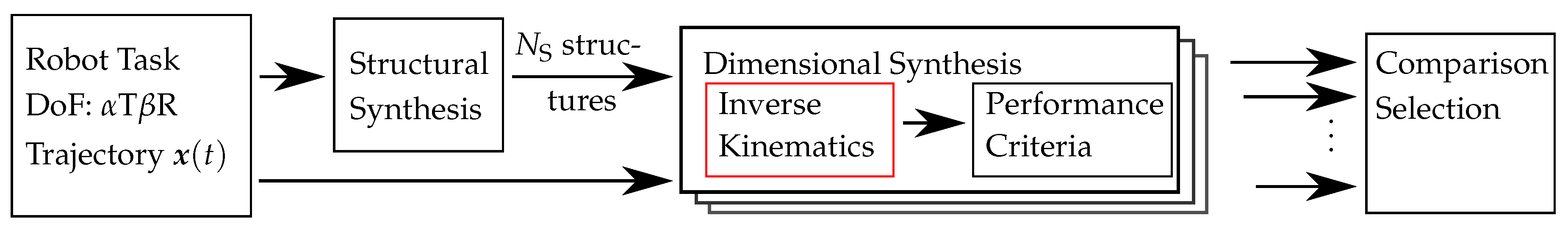
The overview over the literature shows that no general, machine-independent method for the resolution of functional redundancy for 3T3R PKM in 3T2R tasks exists. The works either focus on a general structural synthesis of machines, e.g., via screw theory [31] or linear transformations [29] or the description and improvement of specific, manually selected machines. To choose the best machine for given requirements, a structural synthesis is only the first step. Additionally, a dimensional synthesis should be performed for all possible structures to select the most suitable mechanism. This combined structural and dimensional synthesis [34] is sketched in Figure 2. To be able to perform the dimensional synthesis for all structures, the inverse kinematics has to be implemented in a general form to calculate the performance criteria over a given trajectory for further optimization of the structures and their comparison. For the generation of task redundant parallel robots, the inverse kinematics has to include an optimization of the performance criteria and the restrictions such as joint limits to ensure a comparability of the results.
To address this, the contributions of this paper are
- a general kinematics model for parallel robots using the concept of reciprocal Euler angles [5],
- a complete elimination of the redundant operational space coordinate in this formulation for 3T2R tasks allowing a nullspace optimization in the gradient-based inverse kinematics,
- proofs, examples and simulations to show the performance for single serial kinematic leg chains and complete parallel robots.
The remainder of the paper is structured as follows: The description of the inverse kinematics problem and prior definitions are given in Section 2 and the concept of reciprocal Euler angles from [5] is adapted in Section 3 for parallel robots. This leads to the full kinematic constraints of parallel robots in 3T2R tasks, introduced in Section 4 and applied to the differential kinematics in Section 5. The theoretical analysis is followed by examples and simulations in Section 6. The appendix contains proofs and additional details on the mathematical formulation.
2. Inverse Kinematics Problem for Parallel Robots
Before addressing the specific model for parallel robots in 3T2R tasks in the next section, the standard kinematics model of parallel kinematic machines (“PKM”) is repeated in the following, corresponding to the state of the art [11,15,35] and serving as a reference to highlight its shortcomings for 3T2R tasks. The regarded parallel robot consists of m legs, which each have the joint coordinates . All joints are considered to be single-DoF and additionally to the active joints explicitly all passive joints at the base and at the platform are included in the coordinates of leg i. The coordinates
of the end-effector platform describe the position and orientation of the end-effector frame with respect to the base frame . In the equations, this is marked with left subscript “” for vectors and left superscript “0” for rotation matrices. The platform-related end-effector frame is the desired frame in the inverse kinematics problem and is therefore abbreviated with “D”. The position
is defined as the origin of the platform frame and the rotation matrix
of the platform frame is expressed with Euler angles
as a minimal representation of the orientation coordinates. The symbol “” will be used to denote orientations relative to the base frame throughout this paper. The convention
is used for the Euler angles without loss of generality. The relation between joint coordinates and platform coordinates is established with the kinematic constraint equations, for which most commonly the vector loop
between the position of the platform coupling point relative to the base coupling point is used for each leg chain i [15]. The second term corresponds to the forward kinematics of the serial leg chain. The vector
includes the term that depends on the full orientation of the end-effector. For the bigger part of existing parallel robots, the passive joint coordinates can be eliminated analytically from Equation (6), e.g., by using the Euclidean distance for UPS or RPR leg chains or via trigonometry for RRR chains. This is termed “minimal kinematics set” in [15] and leads to the scalar constraint equation
for each leg i, which can be assembled to the vector of constraint equations
for all m legs of the PKM. The differential kinematics of the PKM is calculated with the time derivative
where the passive joint coordinates do not occur, since they have been eliminated in a previous step. Following [11] to avoid the term “Jacobian” for the elements of (10), the inverse-kinematics matrix
of this model has diagonal form and the direct-kinematics matrix
is fully populated. This definition of the constraints has the following drawbacks:
- The velocity-based theory of linear transformations used by [11] allows determining the mobility of arbitrary parallel robots. The linear transformation is generalized in [12] to accuracy and stiffness modeling by means of screw theory resulting in the “generalized Jacobian”. Both concepts are similar to (10) and do not provide a direct appliance to solve the IKP, since this requires a formulation of the orientation at position level, not velocity level.
- Exploiting the reduction of end-effector coordinates for 3T2R tasks is not possible, since all end-effector coordinates are included in (7).
An alternative kinematic model to encounter the combination of these points is presented in the next section, where the concept of reciprocal sets of Euler angles for the inverse kinematics problem for serial-link robots [5] is transferred to the leading leg of parallel robots.
3. Reciprocal Sets of Euler Angles for the Kinematics of a Serial Leg Chain
To take the rotational symmetry around the tool axis in 3T2R tasks into account, a new set of task space coordinates
has to be defined. The translational part
remains unchanged relative to the operational space coordinates . The rotational part
only contains the first two rotational coordinates of . The last operational space coordinate , the rotation around the z-axis of , is excluded from the task space by the selection matrix . To be able to set the rotational DoF around the tool axis in 3T2R tasks arbitrarily and use gradient-based inverse kinematics, has to be eliminated completely from the kinematics Equations (6). To simplify the following elaborations, the platform frame is still identified as the desired frame of the inverse kinematics problem and the end-effector frame that results from the joint angles of leg i is now termed , which corresponds to the forward kinematics of the leg chain. For a formulation without the tool axis rotation, a different constraint definition
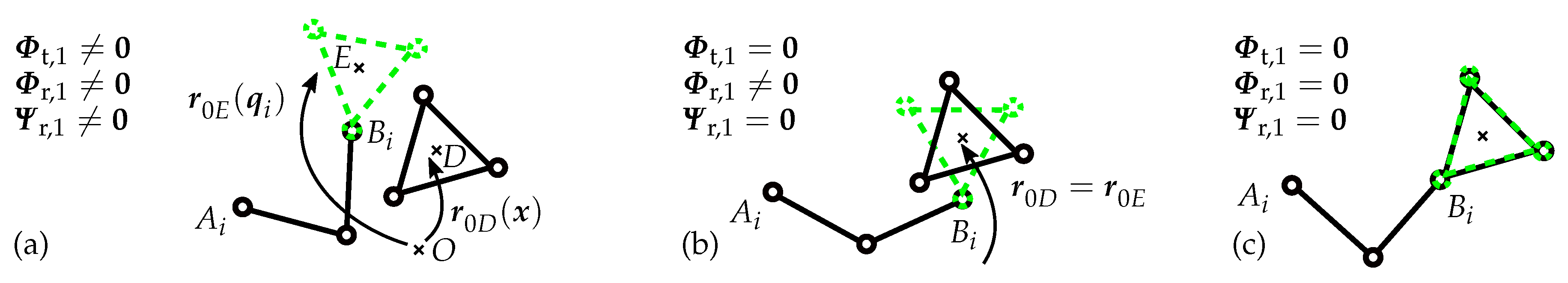
containing the vector loop from the robot base frame to the platform and the leg chain end-effector can be used, where in contrast to (6) only the translational part of the end-effector coordinates appears and not the rotational part . The vector loop is depicted in Figure 3 for a planar robot with opened (Figure 3a,b) and closed loops (Figure 3c). The triangle represents the end-effector platform and only one leg chain is drawn in the figure.
As a drawback of (16), all joint angles of the leg i and not only the coordinates of the first joints counted from the base are now included in the vector
This implies that the platform is now part of the last link of the considered leg chain, as sketched in Figure 3 by the dashed triangle. To account for the increased number of included joints in (17), the full kinematic constraints
have to be considered, including the rotational part
which is needed to generate enough equations for an invertible matrix in the differential equations. The constraints again contain the deviation between the desired end-effector frame expressed with and the actual robots end-effector frame expressed with . Figure 3b,c show cases, where the translational constraints are met, but the rotational constraints have different values. For 3T3R tasks, only Figure 3c represents a valid solution of the inverse kinematics. For 3T2R tasks, Figure 3b,c represent valid solutions.
The goal of eliminating the tool rotation from the equations is not achieved yet, since all three components of the platform orientation affect the rotation matrix . This can be addressed by the selection of the Euler angles: Similar to the definition of the rotational operational space coordinates in (4), the constraints are also expressed with a set of Euler angles . In the following, “” will always refer to the rotation error/residual and “” to an orientation relative to the base frame. The Euler angle convention of can be chosen independently of the choice for the orientation representation in . The intuitive approach of choosing
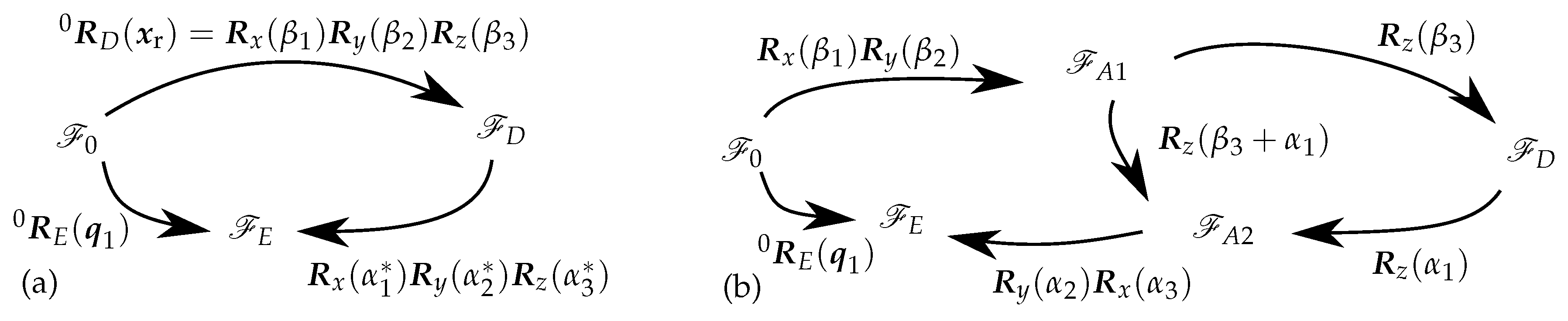
the same way as leads to a set of transformations depicted in Figure 4a, where the intermediate steps of the single elementary rotations are omitted since they have no technical meaning. The superscript asterisk in (20) demarcates this specific example and the following elaborations on the calculation of .
To be able to remove the redundant coordinate from the rotational constraints of (19), it is necessary to change the expression of the orientation error to be reciprocal to the expression of the absolute orientation . By using the Euler angles with
only the error component is affected by rotations around the tool axis, which is the z-axis of the intermediate frames , and the platform frame in Figure 4b, where the frame rotations with the reciprocal set of Euler angles are sketched.
The mathematical proof is given in Appendix A.1 and in [5]. The new, reduced rotational part of the kinematic constraints
does not contain the tool rotation any more. The full kinematic constraints
for the reduced coordinates can be used for the inverse kinematics of the leg chain i in 3T2R tasks, where leads to a valid position and orientation of the tool axis. The condition leads to a valid configuration of leg i of the parallel robot in 3T3R tasks. In the following, “” is always used for 3T3R kinematic descriptions and “” for 3T2R. Note that by omitting the corresponding lines in the operational space coordinates and the constraint equations , it is also possible to use the 3T3R approach for systems with reduced mobility of 2T1R, 3T0R and 3T1R platform DoF.
4. Full Kinematic Constraints for Parallel Robots Using Reciprocal Sets of Euler Angles
The definition of the full kinematic constraints (16,19,18) of a single leg chain of the parallel robot from the previous chapter can be used to write the kinematic constraints in a general form. The full kinematic constraint equations can only be defined for 3T3R tasks without further adjustments as
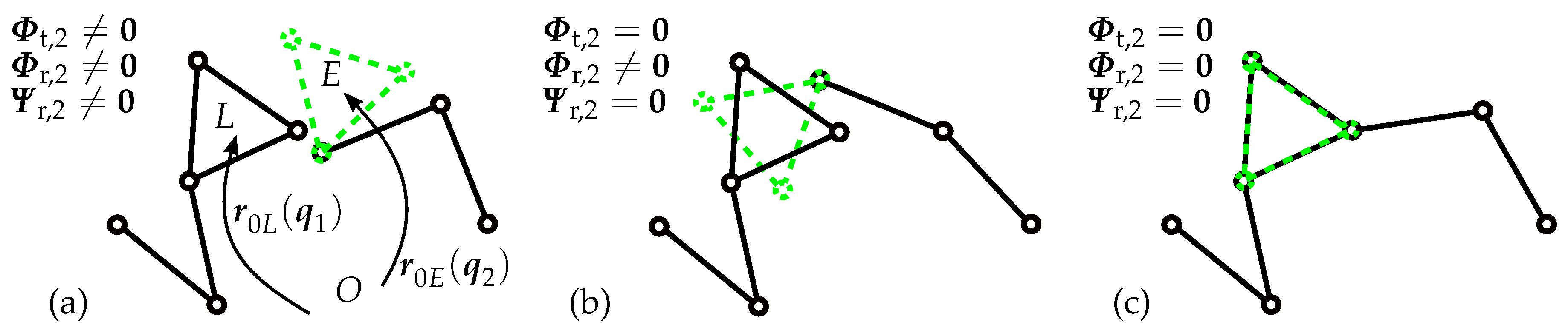
The constraints from (23) for the reduced coordinates can only be defined for one leg chain: Figure 5a show an open-loop second leg chain for a given first leg chain from Figure 3.
By also closing the 3T2R kinematic constraints for the second loop, as depicted in Figure 5b, the tool axis stays arbitrary and the platform pose demanded from the two legs would be different and therefore would not be a valid solution for the complete mechanism, i.e., . Only if the second leg fulfills the 3T3R kinematic constraints for all platform coordinates, as shown in Figure 5c, a valid configuration of the mechanism emerges. This approach has already been used for many specific robots systems, as introduced in Section 1. As a generalization, the first leg of the parallel robot is now termed the “leading leg chain” (index “1”) and the other legs are termed as “following leg chains” (index “j”).
The translational part of the constraints is not coupled by the platform orientation and therefore left unchanged relative to (16) with
for the following legs j.
The orientation for the platform is given with the rotation matrix
which gives the reference end-effector frame resulting from the leading leg 1. The rotational part of the kinematic constraints
for the following leg is given by the Euler angle representation of the deviation between the orientation of the platform frame given by the leading (“L”) leg and the frame given by the respective following leg j. The choice of the Euler angle convention is arbitrary. The full kinematic constraints for the complete parallel robot with m legs for 3T2R tasks
are assembled from the 3T2R constraints from (23) for the leading leg and the 3T3R constraints , from (25,27) for the following legs. The index “j” is used to distinguish the following legs of the 3T2R case and all legs “i” of the general case in Section 3. The full constraints of (28) lead to a 35-dimensional vector for the kinematic constraints for parallel robots with six legs in 3T2R tasks, which are aggregated as class I in Section 1.2. This formulation can be reduced by combining the mechanism-specific approach for the constraints from (6) or (8) with the principle of leading and following legs of this section. For the 6UPS structure this would result in a 10-dimensional constraint vector with five entries for the leading leg and only one entry for each of the five following legs.
5. Differential Kinematics for Parallel Robots
To be able to compute the differential kinematics of the constraints (24) and (28) to
the full inverse-kinematics matrices
and the full direct-kinematics matrices
have to be calculated for the 3T3R and the 3T2R case respectively. The gradient has block diagonal form, indicating that the inverse kinematics problem can be solved for each leg independently. The structures of the gradient results from the coupling of the leading and following joints in the rotational constraints equation.
The gradient matrices and contain nested nonlinear functions related to the orientation error. They are calculated with the chain rule and a syntax for stacking matrix columns to avoid differentiating matrices or with respect to matrices, which was introduced in [5]. The product operator , the stacking operator and the transpose operator used for the implementation in the next section are explained in Appendix A.4.
5.1. Constraint Gradients for the Leading Leg of the 3T2R and All Legs of the 3T3R Case
The constraint definition for the leading leg of the 3T2R case (28) and with for all legs of the 3T3R case (24) are subject to the same model of (16), (19), (18). In the following, the 3T3R constraints are displayed. The form for the 3T2R case is obtained by removing the corresponding line of the rotational component according to (22) and replacing “” by “” in the following equations. For the analysis, the constraint gradient matrix w.r.t. the joint coordinates has to be divided out to
where the translational component can be calculated with the geometric Jacobian of the leg chain, as derived in Appendix A.3. The rotational part is written down as a function composition of the three functions (Euler angles), (matrix product) and (rotation matrix) as
which is then expanded with the chain rule for differentiation and the stack operators to
The two first partial derivatives from (34) are sparse matrices and can be calculated efficiently as shown in Appendix A.4. The factor “I” contains (A24) with and the factor “II” is (A27) with the contents of . The last partial derivative “III” can be derived with computer algebra systems from the analytic expression of the rotation matrix or from the geometric Jacobian, see Appendix A.2. The leading legs constraint gradient matrix w.r.t. the platform coordinates can be expanded in the same manner into
where the definitions from (16) and (19) only leave the rotational part
where the simplicity of the single expression “I”-“IV” is demonstrated in Appendix A.4. The factors are (A24) with in “I”, the permutation matrix for transposition from (A23) in “II”, (A27), where the contents of are inserted in “III” and (A25) with the elements of for in “IV”.
5.2. Constraint Gradients for the Following Leg in the 3T2R Case
As explained regarding (24), the constraints (16) and (19) and their gradients (34) and (36) are used for all legs in the 3T3R case and the leading leg in the 3T2R case. For the following legs in the 3T2R case, the gradients , and with from the right part of (30) and (31) have to be calculated in a similar way. Due to the absence of the platform orientation in (27), (35) simplifies for the following leg to
The gradient w.r.t. the joint coordinates of the following leg contains again the translational part of the legs Jacobian regarding the end-effector platform position in and has the rotational part
which is similar to the expression in (34). The factors of Equation (38) are (A24) with in “I”, (A27), where the elements of have to be inserted in “II” and the partial derivative of the platform orientation calculated from leg j w.r.t. the legs joint coordinates in “III”, similar to term “III” from (34). The gradient w.r.t. the joint coordinates of the leading leg
is similar to the expression in (36). The order of the residual expression (27) has to be switched by exploiting the associative property of matrix transposition to avoid differentiating a transposed matrix. The factors of equation (39) are (A24) with in “I”, the permutation matrix for transposition from (A23) in “II”, (A27) with in “III” and the term “III” from (34) in “IV”.
5.3. Gradient-Based Solution of the Inverse Kinematics Problem with Redundancy Resolution
The presented kinematic constraints and their gradient matrices can be used to solve the inverse kinematics problem (IKP) of single leg chains and complete parallel robots. Since all active and passive joint angles are involved for the case of parallel robots, solving their IKP results in solving the IKP for all leg chains. As first introduced in [7] for Euler angle residuals in the IKP, the Taylor series expansion of leads to the definition of
in an iterative algorithm at the step , which can be used to solve the IKP using a given initial value and the condition
Defining the solution of the IKP as the main task (“T”), the stepwise solution for the joint coordinates results to
Depending on the dimension, denotes the matrix inverse or the pseudo-inverse. Again, the Equations (40)–(42) can be written with “” from (28) instead of “” from (24) for the 3T2R case.
In the latter case, the corresponding gradient matrix from (30) allows defining of a nullspace in the case of . This redundancy can be exploited by using the nullspace (“N”) projection from [6] additionally to the solution of the IKP in (42) with the new increment
in the iterative algorithm. The optimization of additional performance criteria h requires their gradient w.r.t. the joint positions. One criterion is the summed -weighted quadratic distance
of the joint positions from their respective reference position , e.g., used in [2,36]. Defining to be in the middle of the joint limits and minimizing reduces the risk of joints reaching their technical limits, but does not guarantee it, since exceeding the limit for one joint can be compensated by improving other joints. The -weighted hyperbolic joint limit distance
from [8] (written element-wise for ) circumvents this problem by generating infinitely high values when reaching the limits. In contrast to , the criterion is only defined for joints within their limits with , which is ensured by setting for joints exceeding their limits and otherwise. To combine the effect of drawing joint positions to their middle with of (44) and of strongly rejecting joints directly near their limits with of (45), their weighted sum
is used in the simulation studies of Section 6. Other criteria not related to the joint limits are for example stiffness [9] or singularity avoidance via Frobenius norm condition number [8] or squared condition number [4]. The method can be used for serial-link robots as well by removing all entries for the following legs from the formulas, as presented in [5]. The platform pose / corresponds to the desired pose for the serial robots end-effector and the kinematic constraints / correspond to the residual of the IKP.
In the practical implementation, it has proven to be useful to extend the basic principle of (43) to
where the constant damping coefficients for and for were introduced to avoid overshooting of the solution for the prize of slower convergence. The damping term has to be chosen according to the optimization criterion. Further damping was introduced for the 3T2R case with task redundancy to reduce a that would lead to overshoot over the joint limits with . The value is set if no limits would be violated by the increment . For the 3T3R case, is set permanently, since slowing down when approaching the limits does not change the direction of the increment and violating the limits is inevitable. The maximum step size for one iteration was ensured with to stay below 5% of the joint limit range to prevent leaving the validity of the first-order approximation of (40). For smaller increments, holds. The damping terms are always applied to the full vector and not to single elements and therefore only change the norm and not the direction of .
5.4. Differential Kinematics for the Parallel Robot and Its Applications
The reasoning so far only considered the inverse kinematics of the parallel robot. The kinematic definitions can also be used in the differential kinematics (29) to establish the connection between joint and platform velocity. This was already presented in general form in [15] and also corresponds to the theory of linear transformation which is the base of the works of Gogu on structural synthesis [11]. The derivation in this paper is based on the position and orientation, but comes to the same result as the already-existing velocity-based approach. Furthermore, using / as elaborated before allows for the first time defining differential kinematics specifically for 3T2R tasks in a general form. The differential equation of (29) is expanded to
to distinguish active (“a”) and passive (“p”) joints. The latter also contain the coordinates of the platform-connecting joints. Reordering the equation leads to the full inverse differential kinematics
which has been addressed in the previous sections, and the full direct differential kinematics
By only selecting the first rows for in (49) and for in (50), the well-known analytic Jacobian of the parallel robot (called “Euler angles Jacobian matrix” in [15] and “design Jacobian” in [11]), relating actuator velocities and platform velocities , can be obtained from both equations. For the case of task or kinematic redundancy, the pseudo-inverse can be used for in (49) together with a nullspace optimization as shown in Section 5.3. This allows exploiting the functional redundancy in 3T2R tasks also for trajectories , and not only for single poses . When solving the IKP for a trajectory, the IK on position level of Section 5.3 is only needed to correct linearization errors. The case of task redundancy does not affect (50), since the full platform velocity is obtained from given actuator velocities .
6. Results
To evaluate the inverse kinematics (IK) algorithm presented in the previous Section 5.3, first the solution of the IKP is shown for the trajectory of a serial-link industrial robot in Section 6.1 and for the trajectory of a parallel robot in Section 6.2. The results are generalized by the statistical analysis of random point-to-point movements of arbitrary serial link chains in Section 6.3.
6.1. Resolution of Functional Redundancy of a Serial-Link Six-DoF Robot in 3T2R tasks
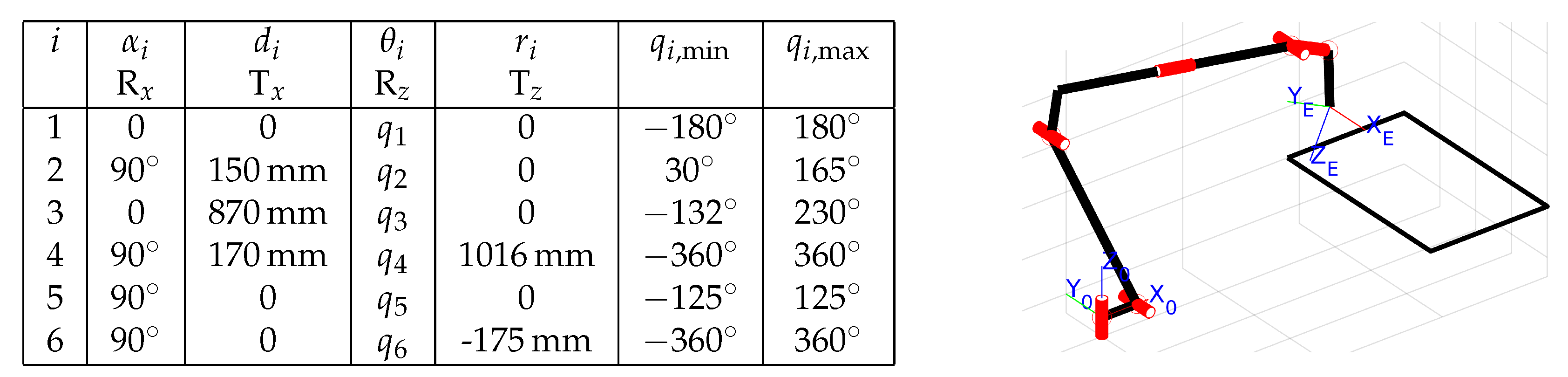
The first evaluation of the IK algorithm from Section 5.3 is performed with simulations at the basic example of a six-DoF industrial robot with a rectangular trajectory with a constant orientation of the z-axis pointing into the ground plane. The manipulator Fanuc M-710 iC/50 was taken from the example of [36] with the tabulated kinematics parameters and a sketch of the trajectory in Figure 6. Deviations in the parameters relative to [36] result from the use of the modified Denavit–Hartenberg notation from [35] for the joint transformations and the use of only positive axis alignment parameters for consistency with the results of the structural synthesis from [34].
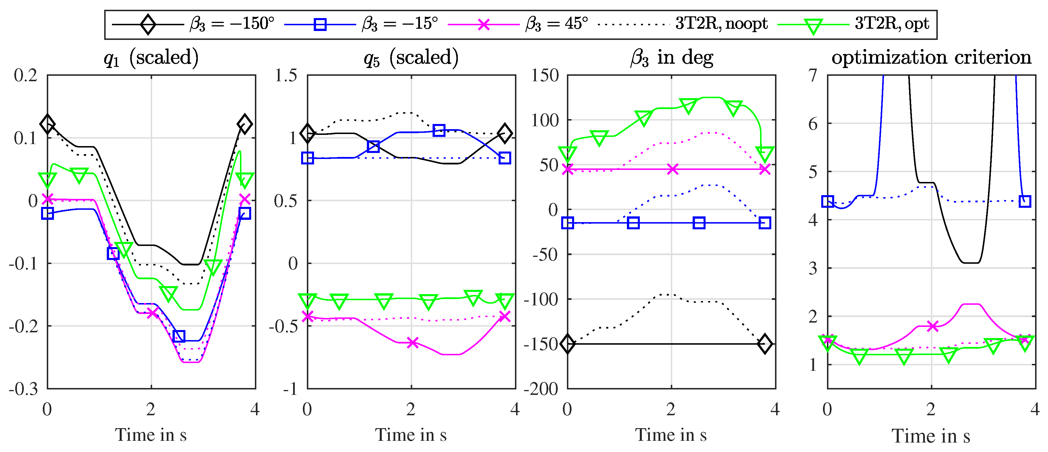
The IKP is solved with two settings: setting the tool axis rotation to different constant values with the 3T3R algorithm and solving the IKP only for the desired pointing direction with the 3T2R algorithm. The algorithm from (43) was used in the extended version of (47) for both cases with different settings caused by their nature. For the 3T3R case, and were set. The terms and have no effect, since no nullspace movement is possible. For the 3T2R case, with and only the hyperbolic limit rejection criterion from (45) was used. The first criterion was not used, since in the trajectory example the limits are not even temporarily exceeded by principle. All IKP algorithms had the same initial value from Figure 6.
The results of the inverse kinematics for different settings are given in Figure 7, where the representative joint coordinates and , the redundant coordinate of the end-effector orientation , as well as the optimization criterion (45) are depicted over time for the trajectory from Figure 6. The positions are normalized to the joint limits from to 1. The first three lines in Figure 7 represent IKP solutions with a given constant end-effector orientation of , and and the 3T3R algorithm. The 3T2R algorithm without nullspace optimization is plotted with dotted lines for each first sample of the 3T3R cases as initial value with the same colors. Using these initial values for a 3T2R IK with optimization leads to strong nullspace movements at the beginning, quickly converging to a local minimum. Therefore, the 3T2R case with optimization, plotted as the green line with triangle markers, is shown only for the initial condition from Figure 6. It can be observed that the optimization of the criterion leads to the best solution of the IKP. The lines for the criterion for and partly exceed the limits of the plot, indicating that the limit is violated, which can also be seen at the plot for . This exposes the need for keeping the solution always within the limits by the measures described. The 3T2R IK without optimization with dotted lines tends to lower changes in the joint positions than the 3T3R IK, since this corresponds to the solution of the matrix pseudo-inverse in (43).
6.2. Resolution of Functional Redundancy of a Parallel Robot in 3T2R Tasks
As elaborated in Section 4 and Section 5, the solution of the IKP for 3T2R and 3T3R tasks is necessary to solve the problem for parallel robots. Therefore, the trajectory evaluation for a 6UPS parallel robot in this section is preceded by the trajectory example for a serial link chain in the previous section. This robot belongs to the first class presented in Section 1.2, which is primarily addressed in this paper.
The robot has a Gough structure [15] with symmetric alignment of the universal joint base couplings on a circle with radius and the spherical joint platform couplings on a circle with radius . The initial pose was set to a center position and the initial orientation was set to zero, meaning an alignment of base and platform frame. The joint positions for each leg were defined to have the initial values for the given initial platform pose to avoid switching within the trajectory and to avoid gimbal lock singularities. The joint limits were set around the resulting zero position to for the prismatic joint and for all single revolute joints representing the universal and spherical joints. The values are higher than typical values for real robots to emphasize the effect of the nullspace movement in a bigger simulated workspace of the robot. The settings for the IK solver are similar to those in Section 6.1, since both cases regard solving the IKP for a trajectory.
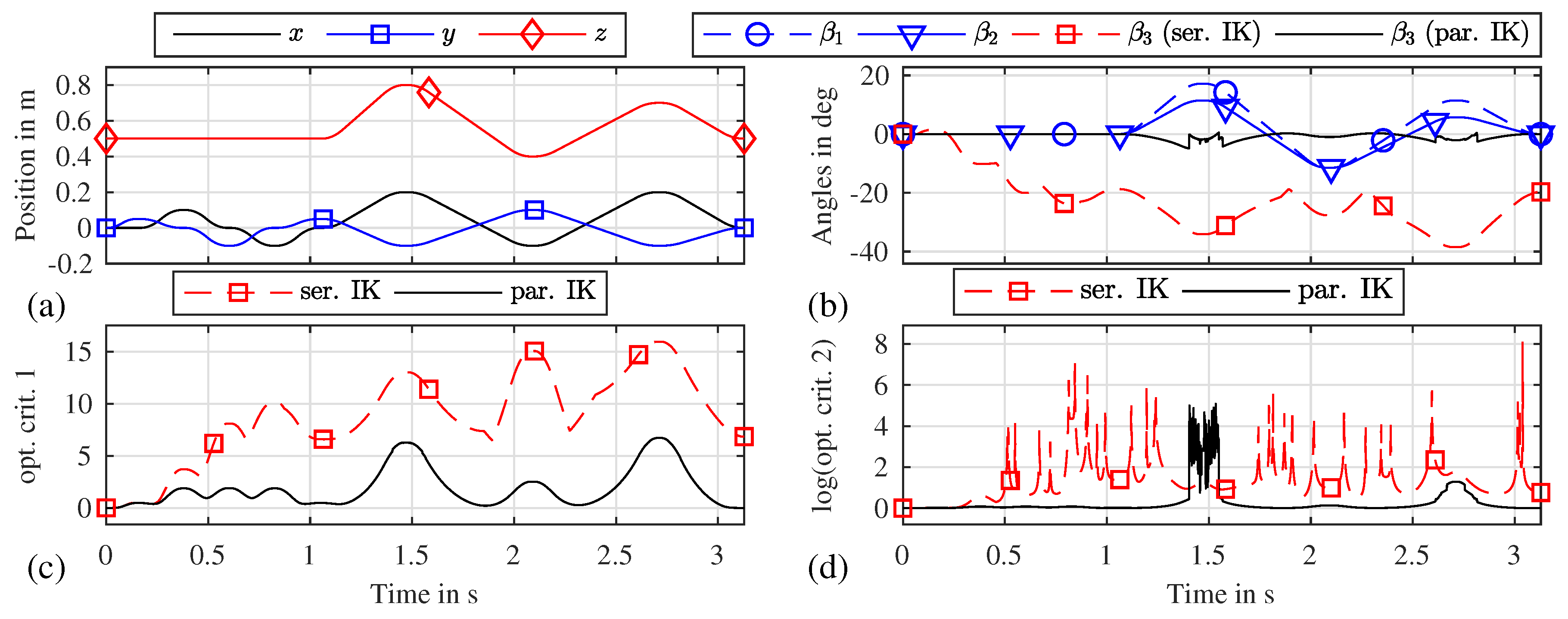
The time evolution of platform pose and optimization criteria is depicted in Figure 8. The reference trajectory can be seen at the platform position in Figure 8a and the platform orientation expressed in Euler angles (-) relative to the base frame in Figure 8b. The IKP is solved using two different methods: Only solving the IKP for the legs separately, called “ser. IK” in Figure 8 and solving the IKP for all legs together, called “par. IK” in Figure 8. Both methods perform an optimization with only of (45), as justified in Section 6.1. The first approach only performs this optimization according to Section 3 for the first leg using the 3T2R method and then solves the IKP for all other legs with the 3T3R method. The second approach uses the optimization for all legs together according to the 3T2R method from Section 4. This results in improved values for the performance criteria depicted for in Figure 8c and for in a logarithmic scale in Figure 8d. Since the first approach does not regard the limits of the following legs, the optimization criterion gives high values indicating many joint limit violations. The second approach only shows peaks at in Figure 8d that result from a joint position getting near to the limit, but not exceeding it. For the practical implementation, the computation time is only weakly influenced by the selection of the method, since calculating the (pseudo-)inverse for six and matrices or one matrix does not present a challenge for current computing hardware. Therefore, the “par. IK” method should be preferred.
6.3. Statistic Results for the Inverse Kinematics of Serial Link Chains
To emphasize the generality of the presented approach, the inverse kinematics is solved for a set of 309 serial kinematic chains with six joints. This set of six-DoF kinematics is generated by permutations of their Denavit–Hartenberg parameters and is reduced with the isomorphism detection of [34] to a minimal set, representing all possible six-DoF serial kinematics with full mobility. The approach is similar to the results of the evolutionary morphology of parallel robot leg chains of [11]. In contrast to the trajectory evaluations in the previous sections focusing on nullspace movement, the inverse kinematics is solved in this section for arbitrary reachable poses of the serial chain in its individual workspace. Therefore, different settings proved to be necessary, since for point-to-point movements, intermediate steps may be outside of the joint limits. In the trajectory case, the initial value for the IKP of the continuous trajectory is always very close to the desired pose of the next trajectory sample. Preventing the algorithm completely from leaving the allowed joint positions reduces the IK success rate. Therefore, the damping term for limit violation was not used in this evaluation, resulting in a constant in (47). To reach again an allowed configuration when approaching the goal pose from intermediate steps with limit violations, the combined criterion from (46) with and was used. Further empirically determined values for all different serial chains were the damping coefficients and in (47). Since these values provide good results for all serial chains with random geometric parameters and for random configurations, they can be regarded as a good choice generally.
To create a general evaluation case, the poses for testing the IK algorithm were generated by the forward kinematics of 50 different joint configurations of the chains uniformly distributed between the joint limits of for revolute joints and for prismatic joints. Additionally, the Denavit–Hartenberg parameters were set to 50 different sets of uniformly distributed parameters between 0 and 1 meters or radians resulting in 2500 combinations for each of the 309 chains in total. The initial value for the solution of the IKP of (47) was set to random values from a uniform distribution within the joint limits. The inverse kinematics was calculated for the full pose with the 3T3R algorithm and only using the pointing direction together with the resolution of functional redundancy in the 3T2R algorithm. A maximum of 15 tries with random initial values was allowed to search for a solution of the IKP within the limits. After that, five more tries were allowed to find a solution violating the limits, but presenting a solution of the IKP to be able to distinguish the two cases, which allows further reasoning on the functionality and possible improvements. A success of the IK is defined as a solution within the joint limits.
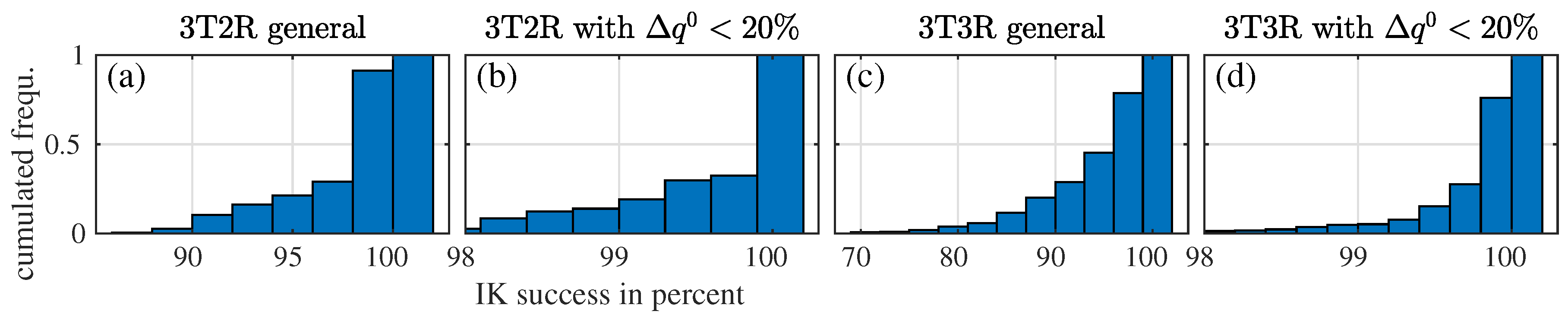
The aggregated results are presented as histograms in Figure 9 for different settings of the algorithm. The histograms show that for the worst case in 3T2R (3T3R) tasks, the success rate is 87% (6%), marked by the position of the first bars in Figure 9a,c. These results can be vastly improved by setting the initial guess within 20% (w.r.t. the joint limit range) around the pose, from which the desired end-effector pose has been calculated. This improves the worst success rate of all kinematic chains to 98% for 3T2R (Figure 9b) and 95% for 3T3R tasks (Figure 9d).
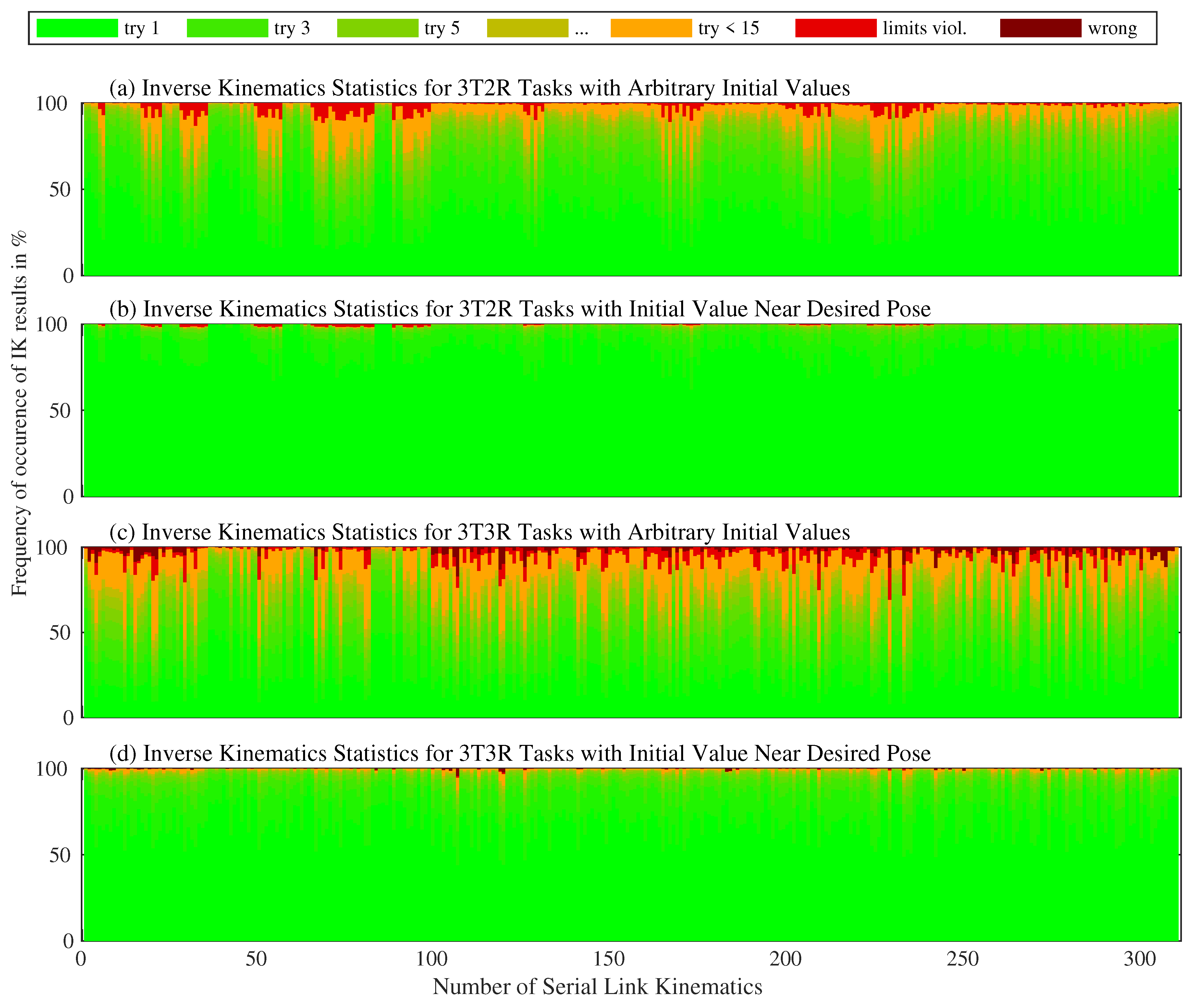
A detailed investigation on the success rates of all possible serial chains is performed in Figure 10.
The 309 serial kinematics are sorted according to their number of revolute joints and are listed on the horizontal axis of the figure: They contain three revolute joints up to no. 98, four R joints up to no. 240, and five R joints up to no. 301. The eight structures from 302 to 309 with six R joints differ in the parallelism of their joint axes. The first 240 kinematic chains with more than one prismatic joint can be seen as a rather academic example and are listed for the sake of completeness. The most prominent chains are the UPS chain from Section 6.2 at no. 266 and the six-DoF industrial robot from Section 6.1 at no. 309. Each bar represents the stacked relative frequency of the IK result state in percent for one kinematic chain. The result state is defined as the number of tries or the success. All bars add up to 100%, which corresponds to the 2500 configurations per chain. Beginning at the bottom, the number of tries necessary for the solution of the IKP is marked with colors from green to orange. Only cases with a violation of the limits (bright red) or wrong position (dark red) correspond to a failure of the algorithm, which has been addressed in the analysis of Figure 9, representing an aggregated form of Figure 10. The subfigures a–d of Figure 10 correspond to the ones in Figure 9. It can be observed that the quality of the results is clustered according to the kinematic groups. Structures with at most one P joint show a considerably better performance of the algorithm with a worst success rate of 97.16% for five R joints and 99.36% for six R joints for the 3T2R case (a), which can be seen at the very small red top parts of the bars in the corresponding range of the diagram. The worse performance of the 3T3R algorithm, mostly caused by limit violations, can be explained by joints changing their configuration, i.e., from “elbow up” to “elbow down”, which causes limit violations but does not affect the 3T3R IK.
7. Discussion
A general kinematics model for parallel robots was introduced to solve the inverse kinematics problem for any kind of parallel robot in tasks with one redundant rotational DoF (3T2R). The prize of the generality of the approach is the increased size of the inverse-kinematics matrices, which is for robots with a simple UPS structure instead of for the non-redundant kinematics and grow up to for general task redundant parallel robots with full mobility. This makes symbolic calculations of the kinematic matrices impossible, allowing only studies on mobility, singularities and other properties of the Jacobian matrix based on numeric calculations. The application of the proposed method can therefore be seen mainly in finding optimal trajectories for task redundant parallel robots in milling or drilling scenarios regarding stiffness, dexterity or joint limits. Due to the performance of the method demonstrated at exemplary cases, an online implementation is possible but has to be proved in future works to converge in real-time conditions for specific machines. The generality of the approach allows using it in a combined structural and dimensional synthesis sketched in Figure 2, extending the purely structural synthesis of parallel robot kinematics from [11,31] to a dimensional synthesis of all structures as shown in [34] for serial robots.
Author Contributions
Conceptualization, M.S. and S.T.; methodology, M.S.; software, M.S.; validation, M.S.; formal analysis, M.S.; writing—original draft preparation, M.S.; writing—review and editing, M.S., S.T., T.O.; supervision, S.T. and T.O.; project administration, T.O.; funding acquisition, S.T. and T.O.
Funding
The financial support from the Deutsche Forschungsgemeinschaft (German Research Foundation, DFG) under grant number OR 196/33-1 is gracefully acknowledged.
Conflicts of Interest
The authors declare no conflict of interest.
Abbreviations
The following abbreviations are used in this manuscript:
| PKM | parallel kinematic machine (parallel robot) |
| IKP | inverse kinematics problem |
| DoF | degrees of freedom |
| xTyR | x translational and y rotational degrees of freedom |
Appendix A. Mathematical Symbols for Reciprocal Euler Angles in Inverse Kinematics
The following appendix contains additional detailed information about the kinematic constraint formulation of this paper. Appendix A.1 contains a mathematical proof for the properties of reciprocal Euler angles in inverse kinematics, which is only outlined in equ. 18 of [5]. The relations of the partial derivatives to the geometric and analytic Jacobian are derived in Appendix A.2 and Appendix A.3. The matrix operations for the partial derivatives are replicated from [5] in Appendix A.4 and the contents of the single partial derivatives are given in Appendix A.5 to facilitate the understanding and implementation by the reader.
Appendix A.1. Proof for the Properties of Reciprocal Euler Angles
This section derives the effect of the reciprocity of Euler angles at the example of the kinematics description of Section 3 and the frames of Figure 4b: An end-effector orientation gives the rotation matrix
which rotates vectors from the actual end-effector frame to the desired or platform end-effector frame . Using the Euler angles and exploiting the properties of rotation matrices yields
as introduced in (5). With an additional rotation around the z-axis for the desired orientation, the resulting new Euler angles are
The additional rotation corresponds to the tool axis defined in Section 3 and leads to a new residual orientation error expressed as a rotation matrix
The first residual orientation error from (A1) corresponding to is defined as a rotation matrix
and as a Euler angle representation
Using the sign-aware operator instead of allows angles to be in , removes ambiguities and provides global differentiability. The second residual corresponding to only differs regarding the additional rotation . Combining (A4) and (A5) leads to
where and . The Euler angles from this rotation matrix are
where only influences the first component . This allows the conclusion that only influences and results in the dependencies
with the consequences for the kinematic modeling of robots in 3T2R tasks described in Section 3.
Appendix A.2. Relation of the Geometric Jacobian and the Partial Derivative of the Rotation Matrix
To be able to calculate the gradient matrices of Section 5, the very uncommon partial derivative of the end-effector rotation matrix with respect to the joint coordinates of the kinematic chain is needed as term “III” in (34) and (38). It can either be derived with computer algebra systems from the analytic expression of the rotation matrix, or by first devising the time derivative
and then performing the derivative w.r.t. . Using the operators of Appendix A.4 on the relation between rotation matrices and angular velocities leads to the formulation
where the end-effector angular velocity can be expressed with the rotational part of the geometric Jacobian. It is used as the argument of the cross product matrix operator in stacked form
Applying again the chain rule for differentiation of the function composition of the three functions (matrix product), (cross product matrix) and (linear relation of velocities), as practiced in Section 5, yields
The first factor is (A28), where the contents of are inserted. The second factor is a sign matrix which can be derived directly from (A13) and only contains 0//1. The third factor is the rotational part of the geometric Jacobian. This completes the calculation of the gradient matrix (34) for the Euler angles orientation residual, which was first introduced, but not pursued further in [7].
Appendix A.3. Relation of the Inverse- and Direct-Kinematics Matrices to the Analytic Jacobian
The properties of the gradient matrices from Section 5 can be illustrated further by comparing them to the analytic Jacobian of one kinematic chain, which gives the platform or end-effector velocity
Also using the differential form (29) for the first kinematic leg chain of the parallel robot gives
and results reorganized to the form of (A15) with (32) and (35) written component-wise to
By equating coefficients of (A15) and (A17) the relations
can be obtained between the gradient matrices and the analytic Jacobian of the serial leg chain. The dependency on and has been added to highlight the main requirement, namely the zero equality condition of (A16): (A18) and (A20) only hold if the orientation residual is zero. In the inverse kinematics procedure of Section 5.3 the residual at step k in (40) is unequal to zero, which means that the Equation (A20) does not hold in this case. The translational part is unaffected, as can be seen by the missing argument in (A19).
Appendix A.4. Matrix Operations for Partial Derivatives
To simplify the calculations of the gradient matrices of the residuals in Section 5, operators for matrices are replaced by operators for vectors, to avoid differentiating matrices or w.r.t. matrices which would require multi-dimensional tensors. The column operator for rotation matrices to stack the coordinate systems unit vectors vertically instead of horizontally is defined as
to avoid differentiating matrices or w.r.t. matrices. The special properties of the group are not exploited and the operator can be used for as well. Matrix multiplication is expressed with the matrix product operator such that
The transposition operator is a permutation matrix such that
Appendix A.5. Contents of the Partial Derivatives
The single expressions derived in Section 5 can be calculated with low computational effort from the definition of the and Euler angles from (5), (21) and (A6). With the gradient “I” in (34), (36), (38) and (39) for angles becomes
and the reciprocal gradient “IV” in (36) for angles yields
with , . The property
can be used to test the implementation, if (A24) and (A25) are defined for the same Euler angle convention.
The gradient of the matrix product (A22) w.r.t. the second factor used in (34)/II, (36)/III, (38)/II and (39)/III is
and to complete the enumeration the gradient w.r.t. the first factor used in (A14)/I is
where are the entries of and the matrices are . By transposing the elements of the matrix product (A22), only the first form (A27) had to be used in Section 5.
References
- Baron, L. A joint-limits avoidance strategy for arc-welding robots. Presented at the International Conference on Integrated Design and Manufacturing in Mechanical Engineering, Montreal, QC, Canada, 16–19 May 2000; note: the paper is not part of the conference proceedings published by Springer. Available online: https://www.researchgate.net/profile/Luc_Baron (accessed on 2 August 2019).
- Huo, L.; Baron, L. Kinematic inversion of functionally-redundant serial manipulators: Application to arc-welding. Trans. Can. Soc. Mech. Eng. 2005, 29, 679–690. [Google Scholar] [CrossRef]
- Žlajpah, L. On orientation control of functional redundant robots. In Proceedings of the IEEE International Conference on Robotics and Automation (ICRA), Singapore, 29 May–3 June 2017; pp. 2475–2482. [Google Scholar] [CrossRef]
- Léger, J.; Angeles, J. Off-line programming of six-axis robots for optimum five-dimensional tasks. Mech. Mach. Theory 2016, 100, 155–169. [Google Scholar] [CrossRef]
- Schappler, M.; Tappe, S.; Ortmaier, T. Resolution of Functional Redundancy for 3T2R Robot Tasks using Two Sets of Reciprocal Euler Angles. In Advances in Mechanism and Machine Science, Proceedings of the 15th IFToMM World Congress on Mechanism and Machine Science, Kraków, Poland, 30 June–4 July 2019; Springer: Berlin, Germany, 2019; Volume 73, pp. 1701–1710. [Google Scholar] [CrossRef]
- Yoshikawa, T. Analysis and control of robot manipulators with redundancy. In Robotics Research: The 1st International Symposium; MIT Press: Cambridge, MA, USA, 1984; pp. 735–747. ISBN 0262022079. [Google Scholar]
- Goldenberg, A.; Benhabib, B.; Fenton, R. A complete generalized solution to the inverse kinematics of robots. IEEE J. Robot. Autom. 1985, 1, 14–20. [Google Scholar] [CrossRef]
- Zhu, W.; Qu, W.; Cao, L.; Yang, D.; Ke, Y. An off-line programming system for robotic drilling in aerospace manufacturing. Int. J. Adv. Manuf. Technol. 2013, 68, 2535–2545. [Google Scholar] [CrossRef]
- Guo, Y.; Dong, H.; Ke, Y. Stiffness-oriented posture optimization in robotic machining applications. Robot. Comput. Integr. Manuf. 2015, 27, 367–376. [Google Scholar] [CrossRef]
- Tale-Masouleh, M.; Gosselin, C. Singularity analysis of 5-RPUR parallel mechanisms (3T2R). Int. J. Adv. Manuf. Technol. 2011, 57, 1107–1121. [Google Scholar] [CrossRef]
- Gogu, G. Solid Mechanics and Its Applications. In Structural Synthesis of Parallel Robots, Part 1: Methodology; Springer: Berlin, Germany, 2008; Volume 866. [Google Scholar]
- Huang, T.; Liu, H.; Chetwynd, D. Generalized Jacobian analysis of lower mobility manipulators. Mech. Mach. Theory 2011, 46, 831–844. [Google Scholar] [CrossRef] [Green Version]
- Merlet, J.P.; Perng, M.W.; Daney, D. Optimal trajectory planning of a 5-axis machine-tool based on a 6-axis parallel manipulator. In Advances in Robot Kinematics; Springer: Berlin, Germany, 2000; pp. 315–322. [Google Scholar] [CrossRef]
- Hong, K.S.; Kim, J.G. Manipulability analysis of a parallel machine tool: application to optimal link length design. J. Robot. Syst. 2000, 17, 403–415. [Google Scholar] [CrossRef]
- Merlet, J.P. Solid mechanics and its applications. In Parallel Robots, 2nd ed.; Springer: Berlin, Germany, 2006; Volume 128. [Google Scholar]
- Zhang, D. Parallel Robotic Machine Tools; Springer: Berlin, Germany, 2009. [Google Scholar]
- Wang, J.; Gosselin, C.M. Kinematic analysis and singularity representation of spatial five-degree-of-freedom parallel mechanisms. J. Robot. Syst. 1997, 14, 851–869. [Google Scholar] [CrossRef]
- Zhang, D.; Gosselin, C.M. Kinetostatic modeling of N-DOF parallel mechanisms with a passive constraining leg and prismatic actuators. J. Mech. Des. 2001, 123, 375–381. [Google Scholar] [CrossRef]
- Zheng, K.J.; Gao, J.S.; Zhao, Y.S. Path control algorithms of a novel 5-DOF parallel machine tool. In Proceedings of the IEEE International Conference on Mechatronics and Automation, Niagara Falls, ON, Canada, 29 July–1 August 2005; Volume 3, pp. 1381–1385. [Google Scholar] [CrossRef]
- Gao, J.S.; Sun, H.; Zhao, Y.S. The primary calibration research of a measuring limb in 5-UPS/PRPU parallel machine tool. In Proceedings of the IEEE International Conference on Intelligent Mechatronics and Automation, Chengdu, China, 26–31 August 2004; pp. 304–308. [Google Scholar] [CrossRef]
- Liu, X.; Xu, Y.; Yao, J.; Xu, J.; Wen, S.; Zhao, Y. Control-faced dynamics with deformation compatibility for a 5-DOF active over-constrained spatial parallel manipulator 6PUS–UPU. Mechatronics 2015, 30, 107–115. [Google Scholar] [CrossRef]
- Wen, S.; Qin, G.; Zhang, B.; Lam, H.K.; Zhao, Y.; Wang, H. The study of model predictive control algorithm based on the force/position control scheme of the 5-DOF redundant actuation parallel robot. Robot. Auton. Syst. 2016, 79, 12–25. [Google Scholar] [CrossRef] [Green Version]
- Mbarek, T.; Nefzi, M.; Corves, B. Prototypische Entwicklung und Konstruktion eines neuartigen Parallelmanipulators mit dem Freiheitsgrad fünf. VDI-Berichte 1892 2005. Available online: https://www.igmr.rwth-aachen.de/index.php/en/rob-en/rob-pentapod-en (accessed on 20 June 2019). (In German).
- Schreiber, H.; Gosselin, C. Analyse et conception d’un manipulateur parallèle spatial à cinq degrés de liberté. In French. Mech. Mach. Theory 2003, 38, 535–548. [Google Scholar] [CrossRef]
- Gao, F.; Peng, B.; Zhao, H.; Li, W. A novel 5-DOF fully parallel kinematic machine tool. Int. J. Adv. Manuf. Technol. 2006, 31, 201. [Google Scholar] [CrossRef]
- Bär, G.F.; Weiß, G. Kinematic Analysis of a Pentapod Robot. J. Geometry Graph. 2006, 10, 173–182. [Google Scholar]
- Lin, W.; Li, B.; Yang, X.; Zhang, D. Modelling and control of inverse dynamics for a 5-DOF parallel kinematic polishing machine. Int. J. Adv. Robot. Syst. 2013, 10, 314. [Google Scholar] [CrossRef]
- Alagheband, A.; Mahmoodi, M.; Mills, J.K.; Benhabib, B. Comparative analysis of a redundant pentapod parallel kinematic machine. J. Mech. Robot. 2015, 7, 034502. [Google Scholar] [CrossRef]
- Gogu, G. Fully-isotropic parallel manipulators with five degrees of freedom. In Proceedings of the 2006 IEEE International Conference on Robotics and Automation, Orlando, FL, USA, 15–19 May 2006; IEEE: Piscataway, NJ, USA, 2006; pp. 1141–1146. [Google Scholar] [CrossRef]
- Huang, Z.; Li, Q.C. General Methodology for Type Synthesis of Symmetrical Lower-Mobility Parallel Manipulators and Several Novel Manipulators. Int. J. Robot. Res. 2002, 21, 131–145. [Google Scholar] [CrossRef]
- Kong, X.; Gosselin, C.M. Type synthesis of 5-DOF parallel manipulators based on screw theory. J. Robot. Syst. 2005, 22, 535–547. [Google Scholar] [CrossRef]
- Tale-Masouleh, M.; Saadatzi, M.H.; Gosselin, C.; Taghirad, H.D. A geometric constructive approach for the workspace analysis of symmetrical 5-PRUR parallel mechanisms (3T2R). In Proceedings of the ASME International Design Engineering Technical Conferences and Computers and Information in Engineering Conference, Montreal, QC, Canada, 15–18 August 2010; pp. 1335–1344. [Google Scholar] [CrossRef]
- Cheng, L.; Wang, H.; Zhao, Y. Analysis and experimental investigation of parallel machine tool with redundant actuation. In Intelligent Robotics and Applications, Proceedings of the International Conference on Intelligent Robotics and Applications, Wuhan, China, 15–17 October 2008; Springer: Berin, Germany, 2008; pp. 179–188. [Google Scholar] [CrossRef]
- Ramirez, D.; Kotlarski, J.; Ortmaier, T. Automatic generation of a minimal set of serial mechanisms for a combined structural—Geometrical synthesis. In Proceedings of the 14th IFToMM World Congress, Taipeh, Taiwan, 25–30 October 2015. [Google Scholar] [CrossRef]
- Briot, S.; Khalil, W. Dynamics of Parallel Robots; Springer: Berlin, Germany, 2015. [Google Scholar]
- Huo, L.; Baron, L. The joint-limits and singularity avoidance in robotic welding. Ind. Robot. 2008, 35, 456–464. [Google Scholar] [CrossRef]
Figure 1.
Typical mechanisms of the different classes. Adapted from [18] (a), [23] (b), [28] (c), [10] (d).

Figure 2.
Overview of the procedure for combined structural and dimensional synthesis.

Figure 3.
Different cases for the kinematic constraints of the leading chain for the 3RRR example: (a) no constraints complied; (b) position and tool axis rotation complied; (c) all constraints complied.
Figure 3.
Different cases for the kinematic constraints of the leading chain for the 3RRR example: (a) no constraints complied; (b) position and tool axis rotation complied; (c) all constraints complied.

Figure 4.
Overview of the different frames (a) for six-DoF tasks with standard Euler angle convention and (b) for five-DoF tasks with reciprocal Euler angle convention; taken from [5].
Figure 4.
Overview of the different frames (a) for six-DoF tasks with standard Euler angle convention and (b) for five-DoF tasks with reciprocal Euler angle convention; taken from [5].

Figure 5.
Different cases for the kinematic constraints of the following chain: (a) wrong position and orientation; (b) correct position and wrong orientation; (c) all kinematic constraints are complied.
Figure 5.
Different cases for the kinematic constraints of the following chain: (a) wrong position and orientation; (b) correct position and wrong orientation; (c) all kinematic constraints are complied.

Figure 6.
Left: Table with the kinematic parameters of the industrial manipulator Fanuc M-710 iC/50. Right: sketch of the robot scenario.
Figure 6.
Left: Table with the kinematic parameters of the industrial manipulator Fanuc M-710 iC/50. Right: sketch of the robot scenario.

Figure 7.
Results of the inverse kinematics with different settings for the trajectory of Figure 6.
Figure 7.
Results of the inverse kinematics with different settings for the trajectory of Figure 6.

Figure 8.
Results of the inverse kinematics of a 6UPS robot in a 3T2R task. (a) platform positions, (b) platform orientation in Euler angles, (c,d) optimization criteria and .
Figure 8.
Results of the inverse kinematics of a 6UPS robot in a 3T2R task. (a) platform positions, (b) platform orientation in Euler angles, (c,d) optimization criteria and .

Figure 9.
Histograms with cumulated frequency of the IK success for all kinematic chains with different settings: 3T2R tasks (a,b) vs. 3T3R tasks (c,d) and arbitrary initial value (a,c) vs. initial near goal pose.
Figure 9.
Histograms with cumulated frequency of the IK success for all kinematic chains with different settings: 3T2R tasks (a,b) vs. 3T3R tasks (c,d) and arbitrary initial value (a,c) vs. initial near goal pose.

Figure 10.
Detailed Statistics of the success of the inverse kinematics algorithm for 3T2R tasks (a,b) and 3T3R tasks (c,d). The Success of the IK solver is shown in different shades of green for increasing numbers of required tries. Different initial values are distinguished in (a,c) and (b,d).
Figure 10.
Detailed Statistics of the success of the inverse kinematics algorithm for 3T2R tasks (a,b) and 3T3R tasks (c,d). The Success of the IK solver is shown in different shades of green for increasing numbers of required tries. Different initial values are distinguished in (a,c) and (b,d).

© 2019 by the authors. Licensee MDPI, Basel, Switzerland. This article is an open access article distributed under the terms and conditions of the Creative Commons Attribution (CC BY) license (http://creativecommons.org/licenses/by/4.0/).
Share and Cite
MDPI and ACS Style
Schappler, M.; Tappe, S.; Ortmaier, T. Modeling Parallel Robot Kinematics for 3T2R and 3T3R Tasks Using Reciprocal Sets of Euler Angles. Robotics 2019, 8, 68. https://doi.org/10.3390/robotics8030068
AMA Style
Schappler M, Tappe S, Ortmaier T. Modeling Parallel Robot Kinematics for 3T2R and 3T3R Tasks Using Reciprocal Sets of Euler Angles. Robotics. 2019; 8(3):68. https://doi.org/10.3390/robotics8030068
Chicago/Turabian StyleSchappler, Moritz, Svenja Tappe, and Tobias Ortmaier. 2019. "Modeling Parallel Robot Kinematics for 3T2R and 3T3R Tasks Using Reciprocal Sets of Euler Angles" Robotics 8, no. 3: 68. https://doi.org/10.3390/robotics8030068
Note that from the first issue of 2016, this journal uses article numbers instead of page numbers. See further details here.