When Low Rank Representation Based Hyperspectral Imagery Classification Meets Segmented Stacked Denoising Auto-Encoder Based Spatial-Spectral Feature

Abstract

When confronted with limited labelled samples, most studies adopt an unsupervised feature learning scheme and incorporate the extracted features into a traditional classifier (e.g., support vector machine, SVM) to deal with hyperspectral imagery classification. However, these methods have limitations in generalizing well in challenging cases due to the limited representative capacity of the shallow feature learning model, as well as the insufficient robustness of the classifier which only depends on the supervision of labelled samples. To address these two problems simultaneously, we present an effective low-rank representation-based classification framework for hyperspectral imagery. In particular, a novel unsupervised segmented stacked denoising auto-encoder-based feature learning model is proposed to depict the spatial-spectral characteristics of each pixel in the imagery with deep hierarchical structure. With the extracted features, a low-rank representation based robust classifier is then developed which takes advantage of both the supervision provided by labelled samples and unsupervised correlation (e.g., intra-class similarity and inter-class dissimilarity, etc.) among those unlabelled samples. Both the deep unsupervised feature learning and the robust classifier benefit, improving the classification accuracy with limited labelled samples. Extensive experiments on hyperspectral imagery classification demonstrate the effectiveness of the proposed framework.

1. Introduction

Hyperspectral imaging collects the spectral information across a certain range of the electromagnetic spectrum at narrow wavelengths (e.g., 10 nm) [1], which makes the resulting hyperspectral image (HSI) a 3D data cube showing spatial-spectral characteristics. In contrast to traditional gray-scale or color images, abundant spectral information makes it convenient for HSIs to detect or identify objects from a cluttered background. Thus, HSIs have been widely employed in many applications, such as resource exploration [2], environment monitoring [3], object recognition [4], biopharming [5], etc.

In these applications, one of the fundamental tasks is the HSI classification, which aims to employ the classifier trained on some observed labelled samples to assign a label to each pixel based on appropriate features. Many HSI classification methods have been proposed [6,7,8,9,10,11]. According to the extraction of features using labelled samples or not, these methods can be roughly divided into two categories, including the supervised feature learning method and the unsupervised feature learning method. A brief review can be found in Section 2.

In the supervised feature learning method, a specific objective function is designed to drive feature learning from labelled samples [12,13]. Recently, witnessing the great success of deep neural networks (DNNs) in various computer vision tasks [14,15], some studies begin addressing HSI classification with DNNs [16,17], where the desired feature and classifier are integrated into a unified mapping function and can be learned from labelled samples via an end-to-end training scheme. More importantly, with the deep hierarchical structure, DNNs enable the learning of more representative features and discriminative classifiers, thus obviously improving the classification accuracy. To this end, extensive labelled samples are needed in training the DNNs. However, labelling pixels in an HSI mainly depends on the experience of experts in geoscience, which is often costly and time-consuming. Therefore, it is crucial in practice to deal with HSI classification with limited labelled samples [18].

When being confronted with limited labelled samples, most studies [19,20] adopt an unsupervised feature learning method, where features are extracted in an unsupervised way (i.e., without using the supervision provided by labelled samples) and then embedded into a supervision-inspired classifier. However, most of these methods suffer from two limitations. On one hand, they often employ a heuristic feature extraction model with shallow structure, which prevents the extracted features from being representative enough for challenging cases (e.g., different materials exhibit similar spectra in an HSI, or vice versa). On the other hand, supervision-inspired classifiers only leverage the information of labelled samples without consideration of the crucial unsupervised correlation provided by those unlabelled samples (e.g., intra-class similarity and inter-class dissimilarity). In other words, this kind of classifier considers the unlabelled samples independently, which makes it difficult to deal with various challenging cases (e.g., sample variation or noise corruption). Both of these limitations hinder those unsupervised feature learning methods from successfully dealing with challenging cases in HSI classification.

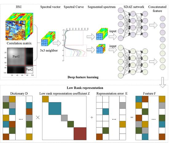
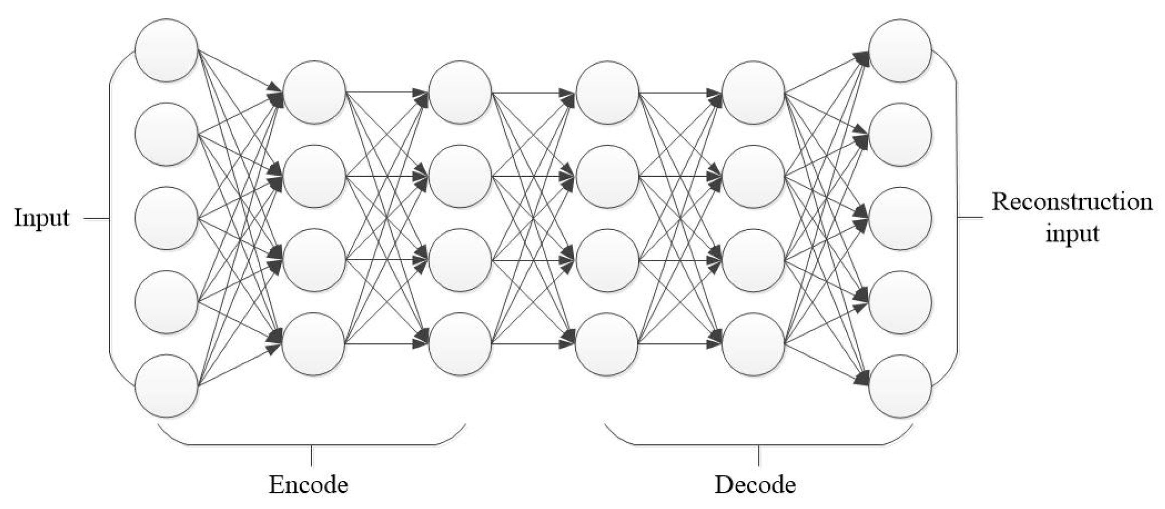
To mitigate these limitations, we present an effective low-rank representation based HSI classification framework. Inspired by the success of the stacked auto-encoder [21] in unsupervised learning, we propose a novel unsupervised segmented stacked denoising auto-encoder-based feature learning model to extract the spatial-spectral characteristics of each pixel in the imagery with deep hierarchical structure. Then, a low-rank representation based classification strategy is developed to incorporate both the supervision information from labelled sample and the unsupervised low-rank property among unlabelled samples into a robust classifier. In the proposed framework, the deep structure of the segmented stacked denoising auto-encoder enables the learning of a complicated feature for each pixel. Moreover, the spatial-spectral setting further increases the representative power of the resulted feature. In the robust classifier, the intra-class similarity and inter-class dissimilarity among unlabelled samples are implicitly captured in classification by exploiting the low-rank property in their representation space, which improves the robustness of the classifier to various challenging cases. Both of these advantages lead to obvious improvements in HSI classification accuracy, especially when the labelled samples are limited. Experiments on two standard HSI classification datasets demonstrate the superiority of the proposed framework over several sate-of-the-art methods.

In general, this study mainly contributes in the following three aspects:

• We propose a novel segmented stacked denoising auto-encoder-based spatial-spectral feature learning model.
• We develop an effective low-rank representation based robust classifier.
• We demonstrate state-of-the-art performance in HSI classification, especially when the labelled samples are limited.

The remainder of this paper is organised as follows. In Section 2, we introduce the related work. Section 3 gives the details of the proposed framework. The experimental results are reported in Section 4. The study is discussed in Section 5. Finally, a conclusion is provided in Section 6.

2. Related Work

In this section, we will briefly review the existing feature learning methods and classifiers for HSI classification. Specifically, those feature learning methods can be divided into supervised methods and unsupervised methods.

Supervised feature learning method. A deep neural network (DNN) is a kind of machine learning method; the basic idea is to build a neural network model containing multiple hidden layers, which needs a large amount of training data to train the network model. There are already many supervised DNN methods [12,14,15,16,17,22,23,24,25,26]. In [22], deep convolutional neural networks (DCNNs) are employed to classify HSIs directly in the spectral domain. In [12], Zhang et al. proposed a dual-channel convolutional neural network-based spectral-spatial classification framework; in this article, a one-dimensional CNN is applied to extract the hierarchical spectral features and a two-dimensional CNN is used to extract the hierarchical spatial features, then a softmax regression classifier is used to combine the spectral and spatial features together and predict classification results. Because deeper neural networks are more difficult to train, in [14], He et al. proposed the image recognition method based on deep residual network (ResNet) to deal with the difficulty of training in DNNs. In [23], a ResNet is built for HSI classification. The back propagation neural network (BP) [27,28] is also a well-known supervised machine learning method, and it has been used in remote sensing image classification [27] and handwritten digit recognition [28]. However, as we all know, most of the supervised feature leaning methods need a large amount of labelled data to train the model, which is always unrealistic when there are only a small number of labelled samples available. Therefore, more and more scholars began to study unsupervised feature learning methods.

Unsupervised feature learning method. Transformation-based feature learning methods [29,30,31,32] map or transfer the original data from the high-dimensional data space into the low-dimensional feature space. The well-known transformation-based characteristics learning methods include principal component analysis (PCA), minimum noise fraction (MNF), etc. PCA [32] can express data in minimum mean square error, but it will be influenced by noise. Therefore, Green et al. [30] and Lee et al. [31] proposed minimum noise separation methods, which arrange the components of the transformation according to the order of signal-to-noise ratio (SNR). Morphological profile-based methods (MPs) are also a kind of unsupervised feature learning method. MPs [33,34] with erosion and dilation operators can capture spatial structures in the images, leading to high classification accuracy. In [33], Li et al. proposed a generalized composite kernel-based method (GCK); first the principal component analysis (PCA) is used to extract the principal components, then the extended multi-attribute morphological profiles (EMAPs) are used to extract spatial information, and lastly the multinomial logistic regression is utilized as the classifier. In addition, the stacked auto-encoder (SAE) is a well-known unsupervised deep feature learning method [21,35]. Considering that the spectrum of the HSI is high and has information redundancy, in order to fully excavate the spectral correlation and reduce the dimensionality, in [21], Zabalza et al. segment the spectral band into different groups and then use different SAE networks to extract the deep features. Unsupervised learning methods have achieved tremendous success, but most of these methods extract features with shallow structure, which limits the representation capacity of the models, so in this study, we extracted deep features with the stacked denoising auto-encoder (SDAE). After the features are extracted, we need a classifier to sign the feature to a certain class label.

Statistical learning-based classifier. Statistical learning is based on a statistical function; it uses the typical representative sample to complete the training of the classification model, lets the classification and recognition system learn the category characteristics, and then classifies according to the classification rules. K-nearest neighbor (KNN), K-means, and iterative self-organizing data analysis technique(ISODATA) are the most common statistical learning methods. In [36], Guo et al. proposed the classification method based on the KNN; in this paper the good value k is determined automatically. In [37], Abbas et al. proposed the classification method based on K-means and ISODATA clustering algorithms. Spectrum matching-based methods directly match a spectrum with the known spectrum in the spectral library or the reference spectrum, then the spectrum is classified according to the matching result. The common methods include spectral encoding match, spectral correlation coefficient, spectral angle match, spectral information divergence method, etc. In [38], Xu et al. proposed the spectral matching approach based on scale-invariant feature transform(SIFT). In [39], Murphy et al. introduced the variable information into the spectral angle match to improve the classification accuracy. In [40], Du et al. first applied spectral information divergence on the hyperspectral image classification; the similarity measure is the probability of spectral information divergence distribution between two pixels. When the spectral information divergence is smaller, the two pixels are more similar. In [41], Baassou et al. combined the dispersion of spatial and spectral information to carry out high spectral image classification. Support vector machine (SVM) [7,42,43,44,45,46] is a typical kernel-based classification method; the basic idea is to map the originally indivisible feature space to the high-dimensional linear separable feature space by kernel function, so as to solve a non-linear classification problem by a linear classification method. Since the dimension of the original data has no effect on the size of the kernel matrix, the kernel function method can effectively deal with the high-dimensional data, thus avoiding the dimension disaster problem of the traditional pattern recognition methods. In addition, logistic regression (LR) [47,48,49] uses the regression function to classify the features into one or multiple classes. These conventional methods can achieve classification tasks easily, but they consider the unlabelled samples independently and neglect the inter-class and intra-class property, which leads to these methods failing to gain robust classification results. Thus, representation based methods gain attention.

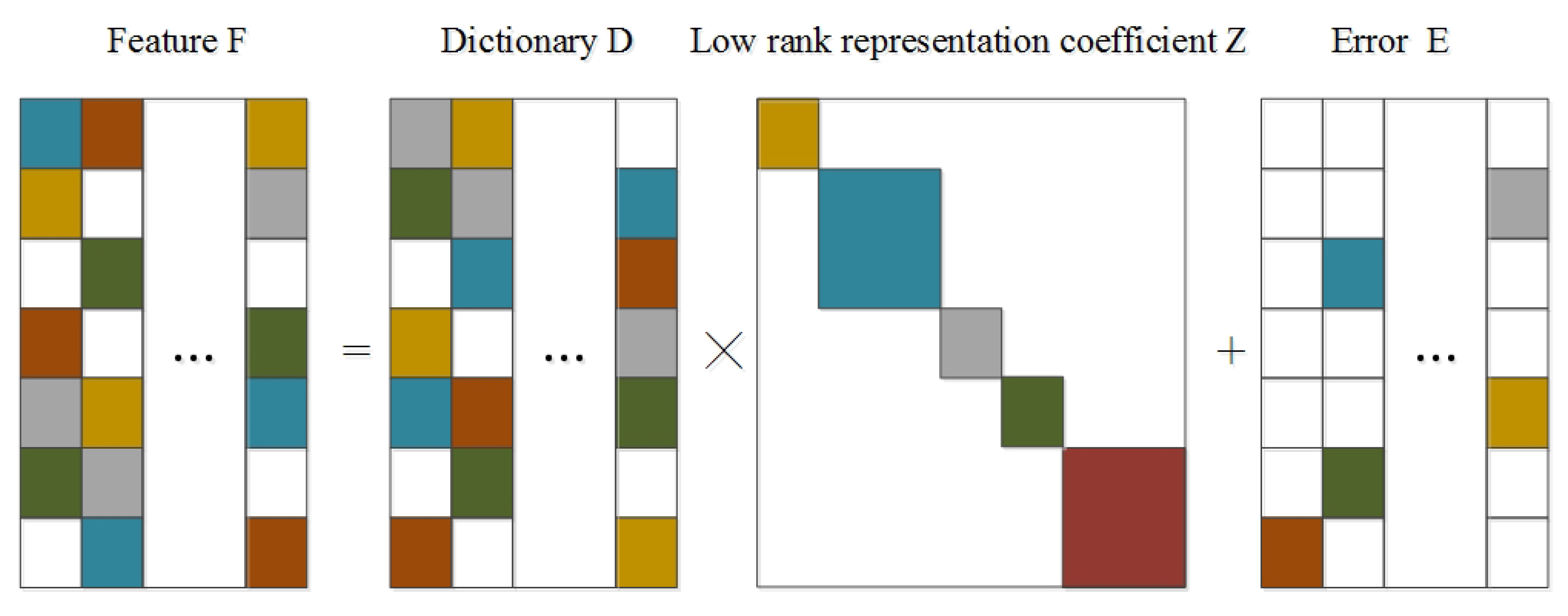
Representation based classifier. Representation based methods [13,50,51,52,53,54,55,56,57,58,59,60,61] implement the classification task by constructing a representation dictionary as a feature subspace and projecting the sample to the feature space, such that the sample is linearly represented by the dictionary atoms. In most cases, only a few of the representation coefficients is not zero, so we also call it a sparse representation based classifier. One class of broadly used representation based methods is structured sparse coding. In [13,57], a sparsity constraint (e.g., $L_1$ norm is used to depict the sparsity, and $L_2$ norm is used to depict the convex) is always added onto a sparse coefficient in the structured sparse coding; there is always some other joint sparsity prior, such as the Laplacian prior. In [50], Wen et al. proposed joint adaptive sparsity and a low-rankness-based online video denoising framework; in this work, the sparse of the vector and the low-rankness of the matrix are considered. Compared with traditional classifiers, representation based methods can better exploit data correlation; in this paper, we develop a classifier based on the representation learning.

3. The Proposed Method

In this section, we will introduce the proposed low-rank representation based hyperspectral imagery classification framework in detail, which mainly consists of two blocks shown as in Figure 1. The deep feature learning block unsupervisedly exploits pixel-wise features with a novel segmented stacked denoising auto-encoder method, and the robust classification block assigns labels to all pixels with a low-rank representation based classifier.

3.1. Notations

Before starting, we will first introduce some notations. A 3D HSI cube is often denoted as $\mathcal{X}\in {\mathbb{R}}^{n_r\times n_c\times n_b}$, which contains $n_r$ rows and $n_c$ columns, and $n_b$ is the band number. In this study, we rearrange the 3D HSI to a 2D matrix $X\in {\mathbb{R}}^{n_b\times n_p}$ for convenience, where each row stacks a vectorized 2D spatial band image with $n_p=n_r\times n_c$ pixels, and each column denotes one spectrum.

3.2. Segmented Stacked Denoising Auto-Encoder-Based Deep Feature Learning

In the segmented stacked denoising auto-encoder-based feature learning, we first divide all spectra into several segments according to spectral correlation, then SDAE is employed on each segment to extract the spatial-spectral feature. Ultimately, we concatenate all features extracted on each segment as a whole feature vector for each pixel.

3.2.1. Spectral Correlation-Based Band Segmentation

HSIs often contain hundreds of spectral bands, which leadS to a continuous spectrum at each pixel, shown in Figure 2. Due to the continuity, a strong correlation exists between bands. Moreover, this kind of correlation varies from band to band. To better exploit the correlation between the different spectral regions of the data, we divide the high-dimensional spectrum into multi-segment low-dimensional spectral vector according to their correlation.

Firstly, for the given HSI X, we define the following covariance matrix $Cov\in {\mathbb{R}}^{n_b\times n_b}$ across the spectral domain as

$$Cov=\mathbf{E}[(X-\mathbf{E}\left(X\right)){(X-\mathbf{E}\left(X\right))}^T],$$

(1)

where $\mathbf{E}$ denotes the mathematical expectation. With the covariance matrix $Cov$, we can further define the correlation matrix $Cor\in {\mathbb{R}}^{n_b\times n_b}$ as follows. Each element $Cor(i,j)$ that depicts the correlation between the i-th band and the j-th band of X can be formulated as

$$Cor\left(i,j\right)=\frac{Cov\left(i,j\right)}{\sqrt{Cov\left(i,i\right)Cov\left(j,j\right)}}.$$

(2)

According to Equation (2), the correlation matrices for the Pavia University dataset and the Indian Pines dataset are shown in Figure 3, where both horizontal and vertical axes represent bands of the dataset. We use color to represent the degree of correlation. Darker indicates less correlation, while lighter represents more correlation. On the basis of the exhibited correlation in Figure 3, we manually divide the spectrum in each dataset into some segments. Specifically, we divide the spectrum of the Pavia University dataset into two segments, including bands 1–75 and bands 75–103. Similarly, the Indian Pines dataset is divided into three segments, namely bands 1–30, bands 30–75, and bands 75–169. It should be noted that we permit a bit of overlapping in different segments.

3.2.2. Deep Spatial-Spectral Feature Extraction

With the band segmentation, we employ the stacked denoising auto-encoder (SDAE) network [20] to extract the deep spatial-spectral feature for each pixel in the given HSI without supervision. The proposed feature extraction method is different from the SDAE proposed in [20], which only extracts the feature from spectral information. Specifically, considering a specific pixel in the HSI, we represent it by all spectra within a $K\times K$ neighbouring region centred at this pixel to collect the raw spatial-spectral information. According to the band segmentation, the representation is divided into several segments. Then, each segment is vectorized into a raw feature vector and fed into the SDAE network to produce the deeply mapped spatial-spectral feature. Ultimately, all deeply mapped features obtained on each segment are concatenated into a final feature vector for the considered pixel. The entire procedure is sketched in Figure 1. In the following, we will briefly introduce how to produce the deeply mapped feature with the SDAE network.

The SDAE network is a prevalent unsupervised learning framework which consists of two symmetric stages, including an encoding stage and a decoding stage. The encoding stage attempts to map the unlabelled input noisy data into a hidden representation through several hierarchical layers, while the decoding stage aims at reconstructing the original clean data by the hidden representation. The architecture of a four-layer SDAE network is shown in Figure 4.

In general, for an SDAE with $2L$ layers (L layers for encoding and L layers for decoding), the encoding operation in the kth encoding layer can be given as

$${f_j}^{(k+1)}=\varphi ({W_j}^{(k+1)}{f_j}^{\left(k\right)}+{b_j}^{(k+1)}),j=1,\dots ,s,k=0,\dots ,L-1,$$

(3)

where ${W_j}^{(k+1)}$ and ${b_j}^{(k+1)}$ denote the weight matrix and the corresponding in bias. s is the number of the segments of the given HSI, and ${f_j}^{(k+1)}$ is the output feature of the jth segment in the kth encoding layer. $\varphi (·)$ denotes the non-linear sigmoid activation function, which is formulated as

$$\varphi \left(x\right)=\frac{1}{1+\exp \left(-x\right)}.$$

(4)

In Equation (3), ${f_j}^{\left(k\right)}$ is the output of the previous layer and ${f_j}^{\left(0\right)}$ is the original input data $x\in X$, the last output ${f_j}^{\left(L\right)}$ is the high-level features which are extracted by the SDAE network; by concatenating the segmented feature ${f_j}^{\left(L\right)}$, we can obtain the final feature F (including the deep feature $F_{train}$ of training data and the deep feature $F_{test}$ of test data).

In the decoding part, the decoding operation in the kth decoding layer can be given as

$${z_j}^{(k+1)}=\varphi ({W_j}^{{}^{\prime }(k+1)}{z_j}^{\left(k\right)}+{b_j}^{{}^{\prime }(k+1)}),k=0,\dots ,L-1,$$

(5)

where ${W_j}^{{}^{\prime }(k+1)}$ and ${b_j}^{{}^{\prime }(k+1)}$ denote the weight matrix and the corresponding in bias in decoding. ${z_j}^{(k+1)}$ denotes the output of the k-th layer. ${z_j}^{\left(0\right)}={f_j}^L$. The output ${z_j}^{\left(L\right)}$ of the last decoding layer is the reconstruction of the original input x.

For simplicity, we denote the SDAE network as $\mathcal{S}(·,\Theta )$, where $\Theta ={\{{W_j}^k,{b_j}^k,{W_j}^{{}^{\prime }k},{b_j}^{{}^{\prime }k}\}}_{k=0,\dots ,L-1}$ collects all parameters. Given N training samples ${\left\{x_i\right\}}_{i=1,\dots ,N}$, the training problem for the SDAE network can be formulated as

$$\underset{\Theta }{\min }\frac{1}{N}\sum _{i=1}^N{∥\mathcal{S}(x_i,\Theta )-x_i∥}^2.$$

(6)

Given the trained SDAE network, we feed an input x into the network; the output of the last encoding layer is considered to be the learned deep feature of x.

3.3. Low-Rank Representation Based Robust Classification

In contrast to the statistic learning-based classifiers (e.g., SVM, KNN), we develop a low-rank representation based classifier which simultaneously exploits the supervision provided by labelled samples and the unsupervised correlation among those unlabelled samples. To this end, we represent the feature matrix $F\in {\mathbb{R}}^{m\times n}$ for all unlabelled samples on a given dictionary D as

$$F=DZ+E,$$

(7)

where $Z\in {\mathbb{R}}^{l\times n}$ denotes the representation coefficient matrix, and $E\in {\mathbb{R}}^{m\times n}$ is the residual matrix.

3.3.1. Structured Dictionary

To benefit from exploiting the unsupervised correlation among unlabelled samples, we construct a structured dictionary $D=[D_1,D_2,\dots ,D_L]$, where the component $D_i\in R^{M\times n_i}$ contains all labelled samples belonging to the i-th class, which is selected from training feature $F_{train}$, and $n_i$ is the number of labelled samples in this class.

3.3.2. Low-Rank Representation

It has been shown that materials from the same category exhibit similar spectra in HSIs, while materials from different categories do not. Figure 5 provides a typical example. Due to the obvious intra-class similarity and inter-class dissimilarity, each sample can be represented well by others in the same class [53], while not by others in another class. Thus, when being represented on the structured dictionary D, samples from the i-th class in F are expected to produce large representation coefficients on the $D_i$ component and small coefficients on other components $D_j$ ($j\ne i$). With appropriate permutation on columns of F (i.e., samples from the same class are gathered into some successive columns), the representation coefficient matrix Z will exhibit obvious diagonal-block structure, shown in Figure 6. Therefore, the supervision from the labelled samples as well as the unsupervised correlation (i.e., intra-class similarity and inter-class dissimilarity) in unlabelled samples can be simultaneously exploited by depicting the underlying block-diagonal structure of Z.

However, the true labels for samples in F are unknown, which makes it intractable to directly reveal the block-diagonal structure in Z. Nevertheless, the underlying block-diagonal structure enables Z to be low-rank [53,54]. Thus, we turn to exploit the low-rank property of Z to implicitly exploit its block-diagonal structure. In addition, due to the intra-class similarity, each sample can be represented well, and the residual matrix E is often sparse. Based on these two points, we give the following low-rank representation framework:

$$\underset{Z,E}{\min }{∥Z∥}_{\ast }+\lambda {∥E∥}_{1}s.t.F=DZ+E,$$

(8)

where the nuclear norm ${∥·∥}_{\ast }$ minimizes the rank of Z to control the structural, $l_1$ norm ${∥·∥}_1$ is utilized to represent the sparsity of the representation error, and $\lambda$ is the balancing weight.

In this study, we employ inexact augmented Lagrange multiplier method to solve the above nuclear norm optimization problem (Equation (8)). Given Z, we can assign the label to a specific sample according to the intra-class similarity with the following classifier:

$$y^i=\arg \underset{l}{\min }{∥f^i-D^l{z}^l∥}_2^2,$$

(9)

where $f^i$ is the feature of the ith sample, $y^i$ is the predict label, $D^l$ is the dictionary of the lth class, $z^l$ is the representation coefficients matrix corresponding to samples $D^l$.

3.4. Low-Rank Representation Based Hyperspectral Imagery Classification Framework

According to the introduction above, the entire flow of the proposed low-rank representation based hyperspectral imagery classification framework can be summarized in Algorithm 1.

Algorithm 1 Low-Rank Representation Based Hyperspectral Imagery Classification with Segmented Stacked Denosing Auto-Encoder Spatial-Spectral Feature

Input: the number of network layers, the number of neurons in each hidden layer, training data, training label, and test data. Obtain segmented spectrum for all training and test data as Equation (2); Train the SDAE networks with the segmented training data, then obtain the deep feature $F_{train}$ of the training data, and $F_{test}$ of the test data as Equation (3); Construct the structured dictionary D with $F_{train}$ and training label; Compute the low-rank representation parameter Z for $F_{test}$ as Equation (8); Predict classification result $y^i$ of each $F_{test}$ as Equation (9); Output: The predict label of the test data.

4. Experiments and Results

4.1. Datasets

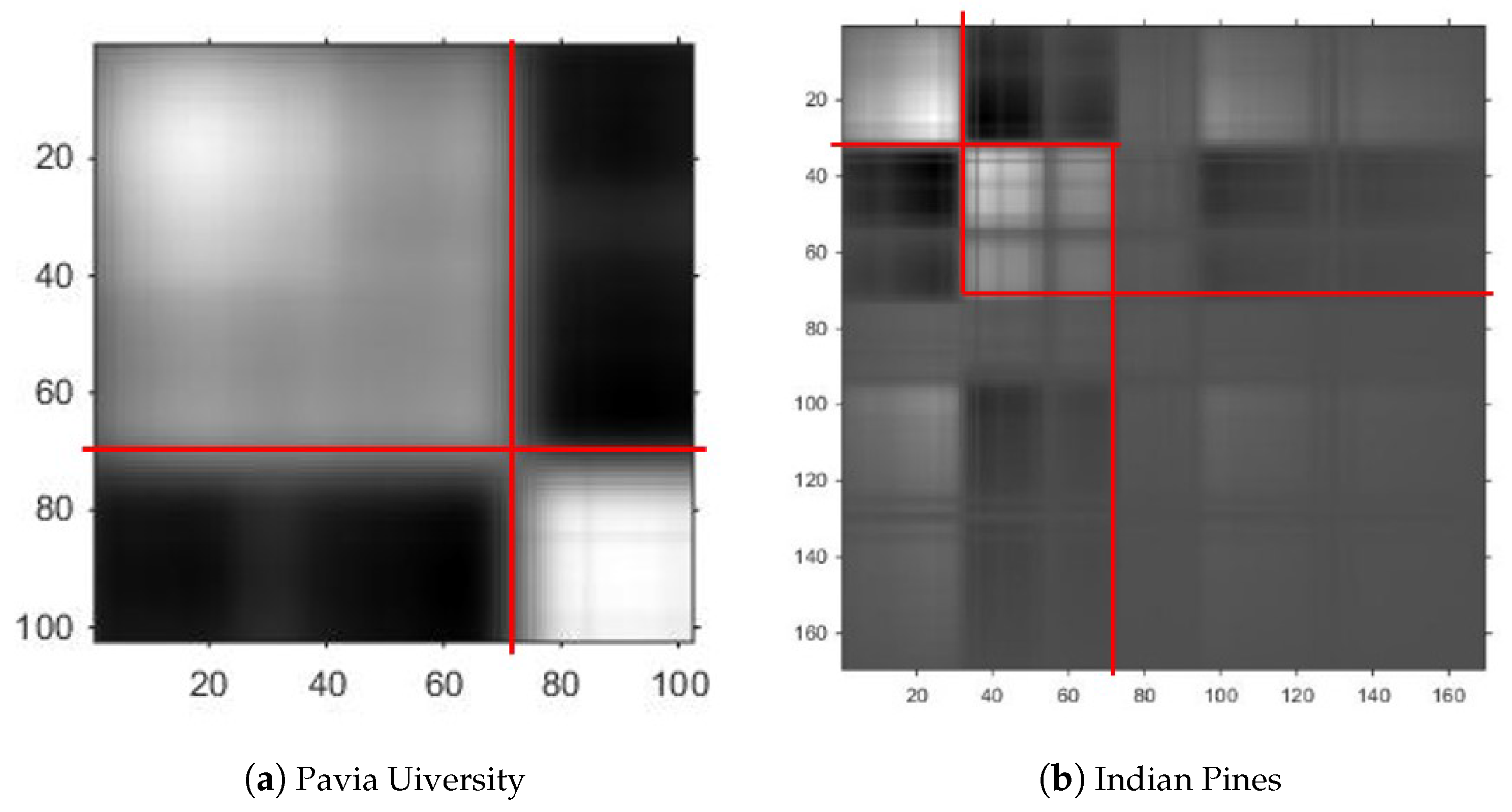
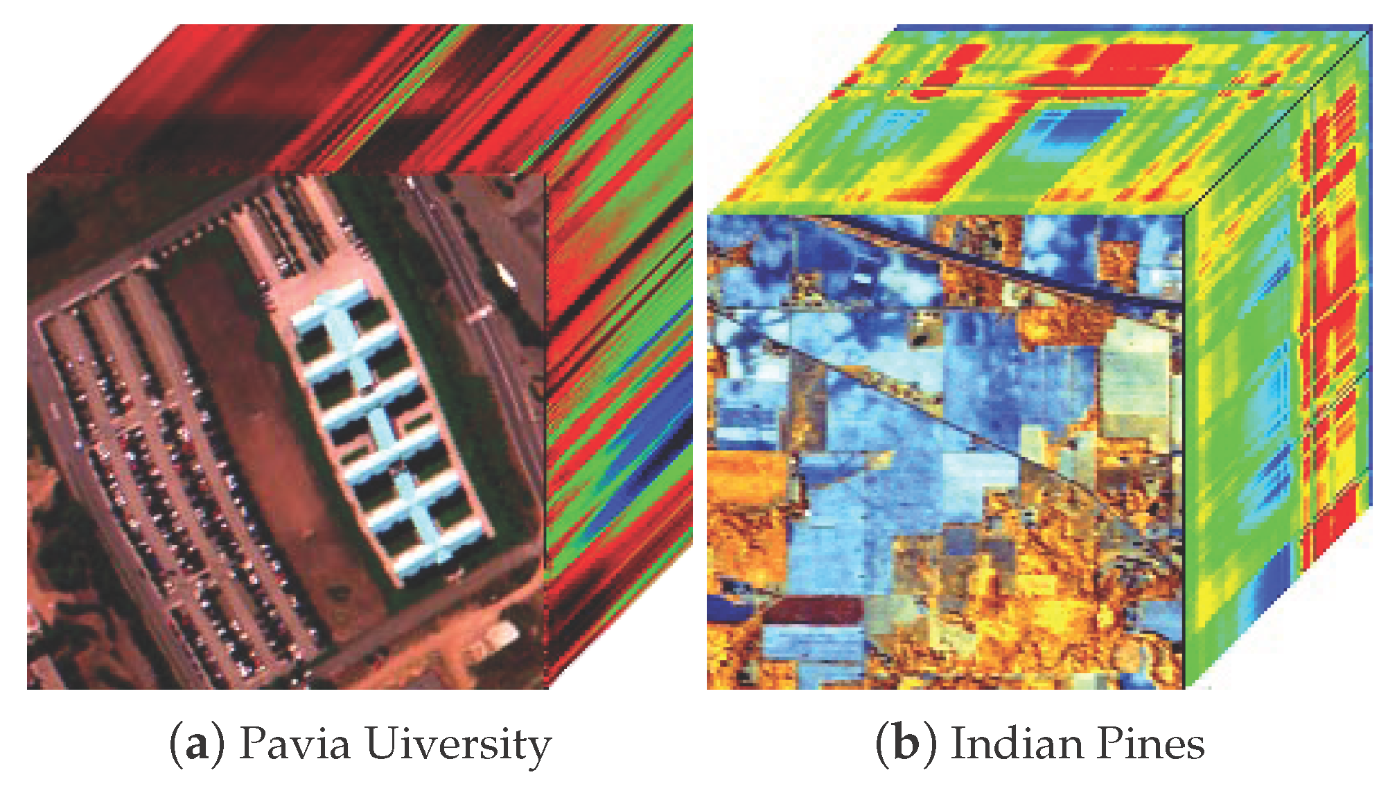
As Figure 7, the Pavia University dataset was collected by the Reflective Optics System Imaging Spectrometer (ROSIS) sensor. The image scenes have 610 × 340 pixels, as collected by the German Aerospace Agency. The dataset has 103 spectral bands. It has a spectral coverage from 0.43 to 0.86 µm and a spatial resolution of 1.3 m. Approximately 42,776 labelled pixels with 9 classes are from the ground truth map, and the numbers of training and test samples are shown in

Table 1. Number of training (labelled) samples and test (unlabelled) samples in the Pavia University dataset.

Number	Class	Training	Test
1	Asphalt	200	6431
2	Meadows	200	18,449
3	Gravel	200	1899
4	Trees	200	2864
5	Metal Sheets	200	1145
6	Bare Soil	200	4829
7	Bitumen	200	1130
8	Bricks	200	3482
9	Shadows	200	747
	Total	1800	40,976

.

The Indian Pines dataset was gathered by the Airborne Visible/Infrared Imaging Spectrometer (AVIRIS) sensor in northwestern Indiana, USA. There are 145 × 145 pixels and 220 spectral channels, the spectral coverage from 0.4 to 2.45 µm including the visible and infrared spectral region with a spatial resolution of 20 m. From the statistical viewpoint, we discarded some classes which only have a few labelled samples and selected nine classes, for which the numbers of training and test samples are listed in

Table 2. Number of training (labelled) samples and test (unlabelled) samples in the Indian Pines dataset.

Number	Class	Training	Test
1	Corn-notill	200	1228
2	Corn-mintill	200	630
3	Grass-pasture	200	283
4	Hay-windrowed	200	278
5	Soybean-notill	200	772
6	Soy-mintill	200	2255
7	Soybean-clean	200	393
8	Woods	200	1065
9	Grass-trees	200	547
	Total	1800	7451

.

4.2. Comparison Methods

To demonstrate the superiority of the proposed method, we compared it with eight state-of-the-art classification methods on HSIs, including SVM [42], Hu’s CNN [22], ResNet [23], SDAE-LR [20], SSAE-SVM [21], GCK [33], and SSDAE-LRR. Among these methods, SVM, SSAE-SVM, GCK, and SSDAE-LRR adopt the unsupervised feature learning scheme, while the others employ an end-to-end training scheme to learn features from labelled samples. Specifically, SVM adopts the raw spectrum as the feature for each pixel. SDAE-LR utilizes the SDAE method to pretrain the network; in the top layer of the network, the logistic regression (LR) approach is utilized to perform supervised fine-tuning and classification. SSAE-SVM employs different SAE on segmented data to extract deep features. The difference from the proposed method is that SSAE-SVM only integrates the spectral information into features without considering the spatial information, and it adopts the SVM as the classifier. Similar to the proposed method, SSDAE-LRR uses different SDAE to extract features, and then a low-rank representation based classifier (LRR) is utilised to classify the feature; when the size K of the neighbouring region is set as 1, the proposed method degrades into SSDAE-LRR.

In implementation, Hu’s CNN and GCK are trained with the codes published by authors, and the other methods are re-implemented by ourselves; the tuned parameters are adopted for best performance.

In the proposed method, the size K of the neighbouring region is set to 3. The number of encoding or decoding layers is changed from 3 to 6; the optimal selection of these parameters is set according to the real test data, the learning rate is 0.1, and the batch size is 20. The deep features that we obtained from Pavia University and Indian Pines were 50 and 20, respectively. Consider a given HSI X, which has s bands; when there are l encoding and decoding layers in the SDAE network, the number of neurons in each hidden layer is $n_1,n_2,\dots ,n_l$, respectively. Hence, the number of parameters is $2\times (s\times n_1+n_1\times n_2+\cdots +n_{l-1}\times n_l)+n_l\times n_l$. For the Pavia University dataset, when training the SDAE network, the number of labelled samples is 1800 and unlabelled samples is 4000, the total parameters are 2.6 × 10⁵ (1.5 × 10⁵ and 1.1 × 10⁵ for each segment). For the Indian Pines dataset, there are 1800 labelled samples and 4000 unlabelled samples used to train the network; the total parameters are 5 × 10⁵ (0.5 × 10⁵, 0.9 × 10⁵, and 3.9 × 10⁵ for each segment).

4.3. Evaluation Metric

To quantitatively evaluate the performance of all methods, we adopted three standard measuring criteria, namely overall accuracy (OA), average accuracy (AA), and KAPPA coefficient. OA denotes the classification accuracy on all testing samples, AA measures the average class-wise classification accuracy across all classes, and the KAPPA coefficient calculates the statistic degree of agreement in classification over the expected results, and is often normalized to 0 and 1. For each criterion, a larger score denotes a better classification result.

4.4. Comparison with State-of-the-Art Methods

In this part, we mainly focus on demonstrating the superiority of the proposed method in terms of classification accuracy over the other comparison methods. To this end, we conducted classification experiments on the two mentioned datasets. The number of training and testing samples are listed in Table 1 and Table 2. To reduce the effect of random sampling on the classification result, we report the average classification results for all methods across 10 rounds with different sampling results.

Table 3. Classification accuracy (%) of different methods on Pavia University dataset (a total of 1800 labeled samples were used for training).

Class	Original-SVM	Hu’s CNN	ResNet	SDAE-LR	SSAE-SVM	GCK	SSDAE-LRR	The Proposed Method
1	$86.75$	$87.34$	$93.17$	$94.01$	$92.54$	$97.57$	$94.47$	$98.35$
2	$92.56$	$94.63$	$96.08$	$95.09$	$91.40$	$99.88$	$95.81$	$99.04$
3	$87.89$	$86.47$	$95.95$	$92.47$	$92.68$	$99.62$	$93.91$	$99.68$
4	$97.17$	$96.25$	$97.77$	$98.85$	$98.53$	$99.71$	$98.57$	$99.23$
5	$99.56$	$99.65$	100	$99.91$	$99.91$	100	100	100
6	$92.86$	$93.23$	$95.55$	$97.14$	$96.44$	$99.98$	$97.84$	$99.03$
7	$93.72$	$93.19$	$97.70$	$98.67$	$98.14$	$99.62$	$97.79$	$99.56$
8	$84.49$	$86.42$	$66.03$	$90.70$	$89.66$	$99.73$	$92.84$	$98.87$
9	100	$99.57$	100	100	100	100	100	100
AA	$92.78\pm 0.16$	$93.02\pm 0.17$	$93.58\pm 0.28$	$96.32\pm 0.06$	$95.48\pm 0.18$	$\mathbf{99.57}\pm \mathbf{0.14}$	$96.81\pm 0.21$	$99.32\pm 0.45$
OA	$91.47\pm 0.96$	$92.56\pm 0.48$	$93.34\pm 0.34$	$95.26\pm 0.42$	$93.16\pm 0.80$	$\mathbf{99.47}\pm \mathbf{0.05}$	$95.91\pm 0.32$	$98.84\pm 0.44$
KAPPA	$88.66\pm 1.19$	$90.68\pm 0.51$	$93.18\pm 0.21$	$95.14\pm 0.43$	$93.01\pm 0.81$	$\mathbf{99.29}\pm \mathbf{0.06}$	$96.01\pm 0.18$	$98.81\pm 0.45$

and

Table 4. Classification accuracy (%) of different methods on Indian Pines dataset (a total of 1800 labeled samples wereused for training).

Class	Original-SVM	Hu’s CNN	ResNet	SDAE-LR	SSAE-SVM	GCK	SSDAE-LRR	The Proposed Method
1	$84.85$	$78.59$	$87.38$	$78.85$	$78.28$	$98.26$	$79.15$	$82.25$
2	$89.12$	$85.23$	$83.33$	$96.85$	$98.42$	$98.08$	$98.42$	$99.37$
3	$98.65$	$95.75$	$97.79$	$99.33$	100	100	100	100
4	$95.98$	$99.81$	$97.86$	$99.82$	$92.50$	$98.26$	$91.77$	$95.43$
5	$99.65$	$99.63$	100	100	100	100	100	100
6	$89.32$	$89.63$	$93.49$	$97.40$	$97.01$	$98.35$	$97.79$	$98.83$
7	$79.23$	$81.55$	$83.63$	$76.32$	$73.24$	$94.73$	$75.97$	$84.10$
8	$94.96$	$95.43$	$91.53$	$94.44$	$94.69$	$98.86$	$95.89$	$97.58$
9	$99.54$	$98.59$	$91.34$	$95.52$	$91.86$	$97.99$	$96.16$	$99.27$
AA	$92.34\pm 0.64$	$91.58\pm 0.04$	$91.82\pm 0.12$	$93.17\pm 1.15$	$91.87\pm 0.81$	$\mathbf{97.91}\pm \mathbf{0.48}$	$92.78\pm 0.73$	$95.20\pm 0.12$
OA	$88.56\pm 0.41$	$87.29\pm 0.29$	$88.94\pm 0.32$	$88.80\pm 2.02$	$86.94\pm 1.54$	$\mathbf{96.91}\pm \mathbf{0.56}$	$88.19\pm 1.15$	$92.16\pm 0.15$
KAPPA	$86.43\pm 0.45$	$84.93\pm 1.02$	$87.04\pm 0.54$	$88.62\pm 1.24$	$86.74\pm 0.03$	$\mathbf{96.31}\pm \mathbf{0.66}$	$88.01\pm 0.87$	$92.03\pm 0.16$

summarize the numerical classification results of all methods on two HSI datasets, where 200 labelled samples per class were used for training (a total of 1800 samples). We can find that the proposed method produced much higher classification accuracy than that of SVM. For example, on the Pavia University dataset, the proposed method outperformed SVM by 7.37% in OA. On the Indian Pines dataset, the proposed method outperformed SVM by 3.60% in OA. This demonstrates that the deeply learned feature performs better than the heuristically shallow feature. Moreover, the proposed method even outperformed the state-of-the-art supervised feature learning method with deep neural networks—Hu’s CNN and ResNet. This is because training deep neural networks with limited labelled samples is prone to becoming trapped in local minima, while the proposed unsupervised deep feature learning scheme have sufficient unlabelled samples for training. Compared with SDAE-LR, SSAE-SVM, and SSDAE-LRR, the proposed method improved the OA by 3.58%, 5.68%, and 2.93% on the Pavia University dataset, and the improvements to Indian Pines dataset was up to 3.36%, 5.22%, and 3.97%, respectively. On the Pavia University dataset and the Indian Pines dataset, GCK outperformed the proposed method by 0.57% and 4.75% in OA, respectively. However, in

Table 5. Classification accuracy (%) of different methods on Pavia University dataset (a total of 100 labeled samples were used for training).

Class	Original-SVM	Hu’s CNN	ResNet	SDAE-LR	SSAE-SVM	GCK	SSDAE-LRR	The Proposed Method
1	$75.15$	$80.41$	$82.94$	$79.41$	$93.84$	$92.26$	$91.60$	$98.86$
2	$72.41$	$57.87$	$62.20$	$95.11$	$92.13$	$92.41$	$94.93$	$98.49$
3	$80.84$	$80.15$	$83.99$	$98.03$	$91.63$	$85.42$	$93.00$	$98.05$
4	$93.71$	$86.63$	$92.18$	$99.09$	$98.95$	$96.70$	$98.67$	$99.16$
5	$99.47$	$98.69$	$99.13$	$99.96$	$99.91$	$99.93$	100	100
6	$62.73$	$91.36$	$87.60$	$94.22$	$96.27$	$99.90$	$97.25$	$98.45$
7	$85.29$	$57.70$	$50.44$	$98.19$	$97.35$	$97.44$	$97.96$	$99.56$
8	$66.11$	$34.16$	$33.76$	$48.89$	$90.98$	$69.93$	$91.18$	$96.61$
9	$99.89$	100	100	100	100	$94.30$	100	100
AA	$81.73\pm 1.24$	$75.22\pm 1.54$	$75.80\pm 2.08$	$90.42\pm 3.99$	$95.67\pm 0.02$	$92.40\pm 0.72$	$96.07\pm 0.72$	$\mathbf{98.81}\pm \mathbf{0.05}$
OA	$74.93\pm 3.87$	$68.16\pm 2.06$	$70.40\pm 1.16$	$90.16\pm 3.58$	$93.57\pm 0.16$	$90.65\pm 2.17$	$94.85\pm 0.84$	$\mathbf{98.31}\pm \mathbf{0.27}$
KAPPA	$68.28\pm 2.63$	$67.49\pm 2.17$	$69.78\pm 1.43$	$89.93\pm 3.66$	$93.43\pm 0.17$	$87.92\pm 2.66$	$94.73\pm 0.56$	$\mathbf{98.27}\pm \mathbf{0.28}$

and

Table 6. Classification accuracy (%) of different methods on Indian Pines dataset (a total of 100 labeled samples were used for training).

Class	Original-SVM	Hu’s CNN	ResNet	SDAE-LR	SSAE-SVM	GCK	SSDAE-LRR	The Proposed Method
1	$52.70$	$29.34$	$37.84$	$60.05$	$70.02$	$54.77$	$74.88$	$79.19$
2	$50.91$	$57.73$	$52.05$	$98.74$	$98.74$	$62.89$	$98.11$	$98.55$
3	$88.68$	$70.71$	$70.37$	$89.23$	$86.53$	$78.56$	100	100
4	$95.24$	$56.31$	$53.02$	$89.03$	$89.40$	$84.87$	$94.15$	$94.52$
5	$98.74$	$95.85$	$93.08$	100	100	100	100	100
6	$73.14$	$61.20$	$76.69$	$89.32$	$88.54$	$69.21$	$93.75$	$97.66$
7	$60.76$	$27.87$	$29.94$	$57.46$	$56.94$	$42.61$	$71.10$	$83.46$
8	$61.53$	$48.07$	$48.55$	$93.96$	$92.27$	$64.09$	$93.96$	$97.58$
9	$82.15$	$67.28$	$59.69$	$30.03$	$94.24$	$79.87$	$96.07$	$98.53$
AA	$73.76\pm 2.13$	$57.15\pm 1.91$	$57.91\pm 3.16$	$78.58\pm 2.16$	$84.92\pm 2.25$	$69.03\pm 3.74$	$91.33\pm 0.74$	$\mathbf{94.26}\pm \mathbf{0.05}$
OA	$69.12\pm 0.80$	$47.18\pm 3.40$	$48.87\pm 4.01$	$66.36\pm 6.78$	$78.57\pm 3.07$	$62.13\pm 7.06$	$86.17\pm 0.89$	$\mathbf{90.80}\pm \mathbf{0.19}$
KAPPA	$64.17\pm 1.01$	$46.45\pm 1.42$	$48.13\pm 2.48$	$65.01\pm 7.74$	$78.25\pm 3.11$	$56.75\pm 3.14$	$85.96\pm 1.72$	$\mathbf{90.65}\pm \mathbf{0.20}$

, when only 100 labelled samples were used for training, the proposed method outperformed GCK by 7.66% and 28.66% in OA on the Pavia University dataset and the Indian Pines dataset. We can conclude that the proposed method outperformed GCK in HSI classification with small labelled samples. These demonstrate the effectiveness of the spatial-spectral deep feature as well as the robust low-rank representation based classifier.

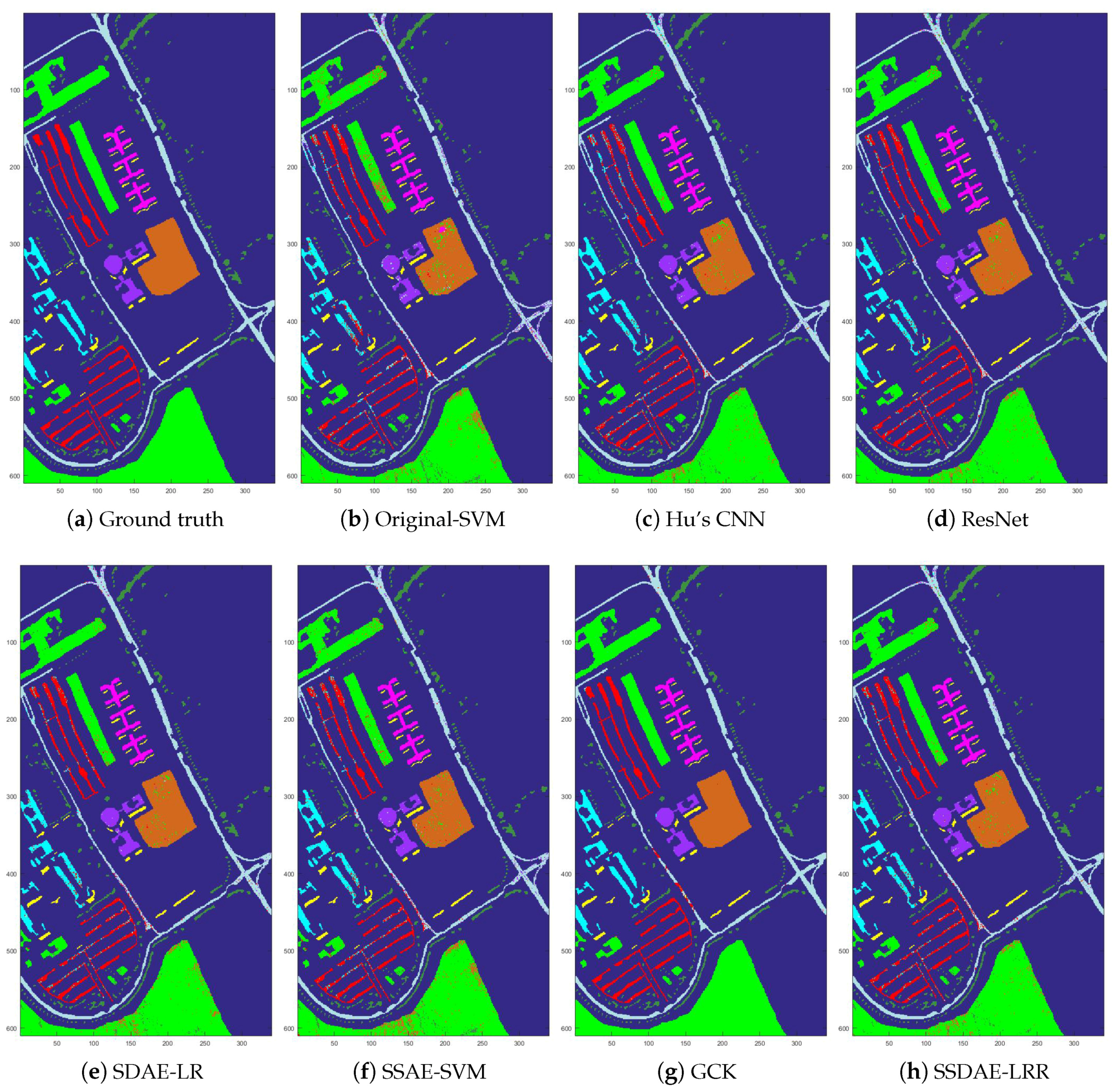
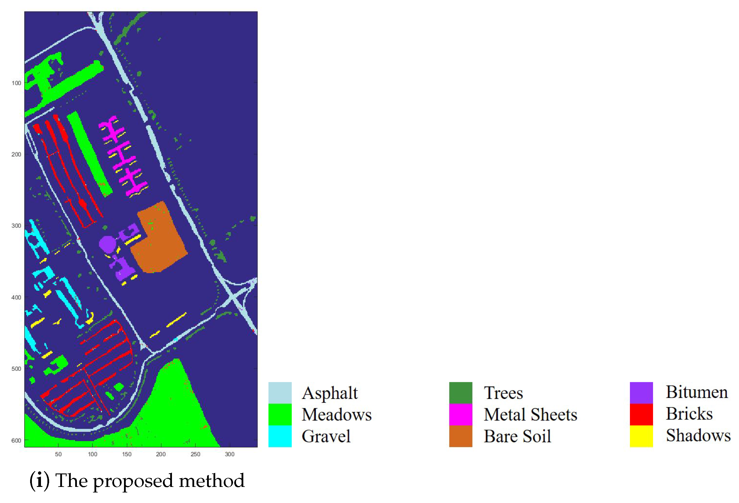
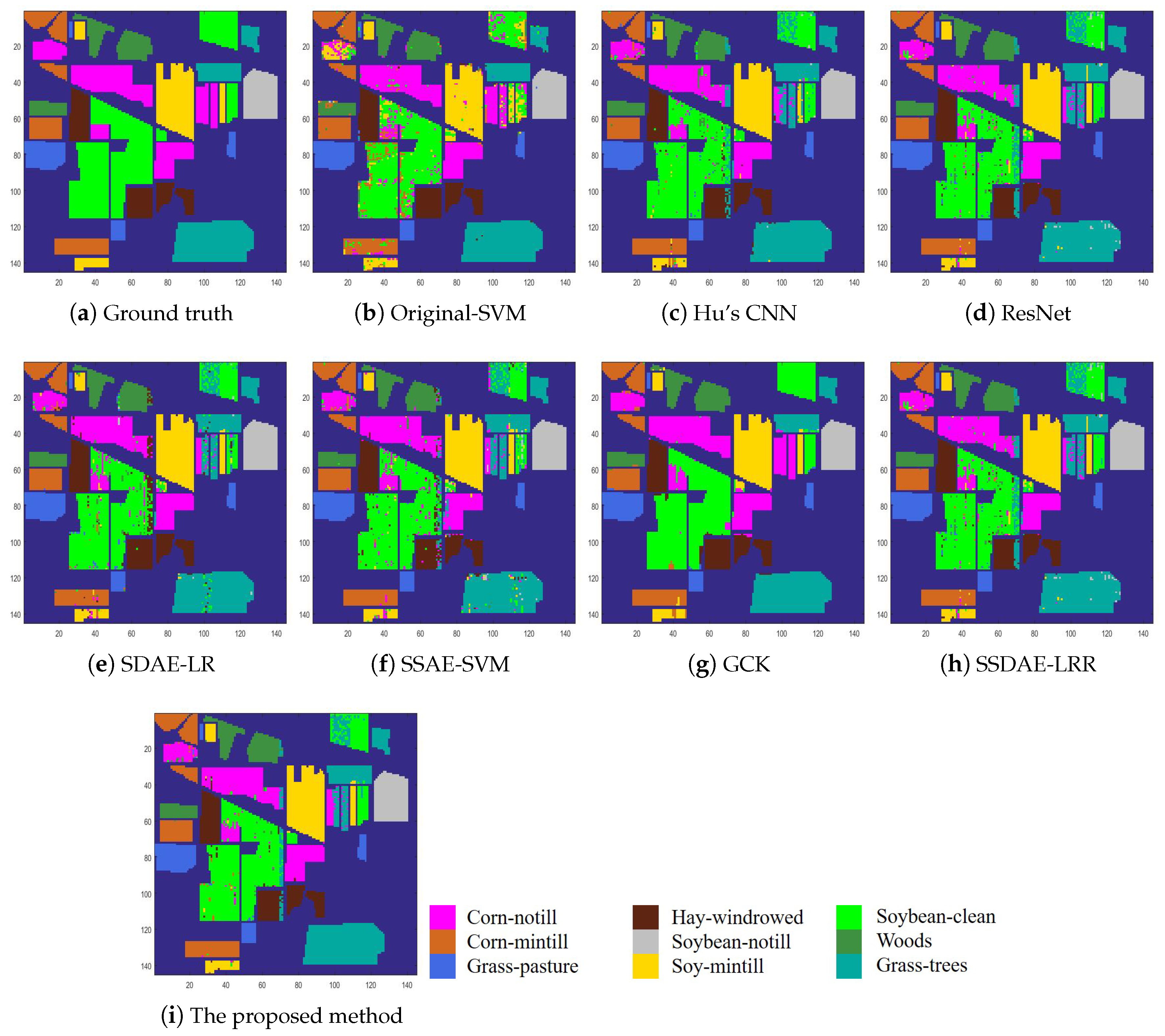
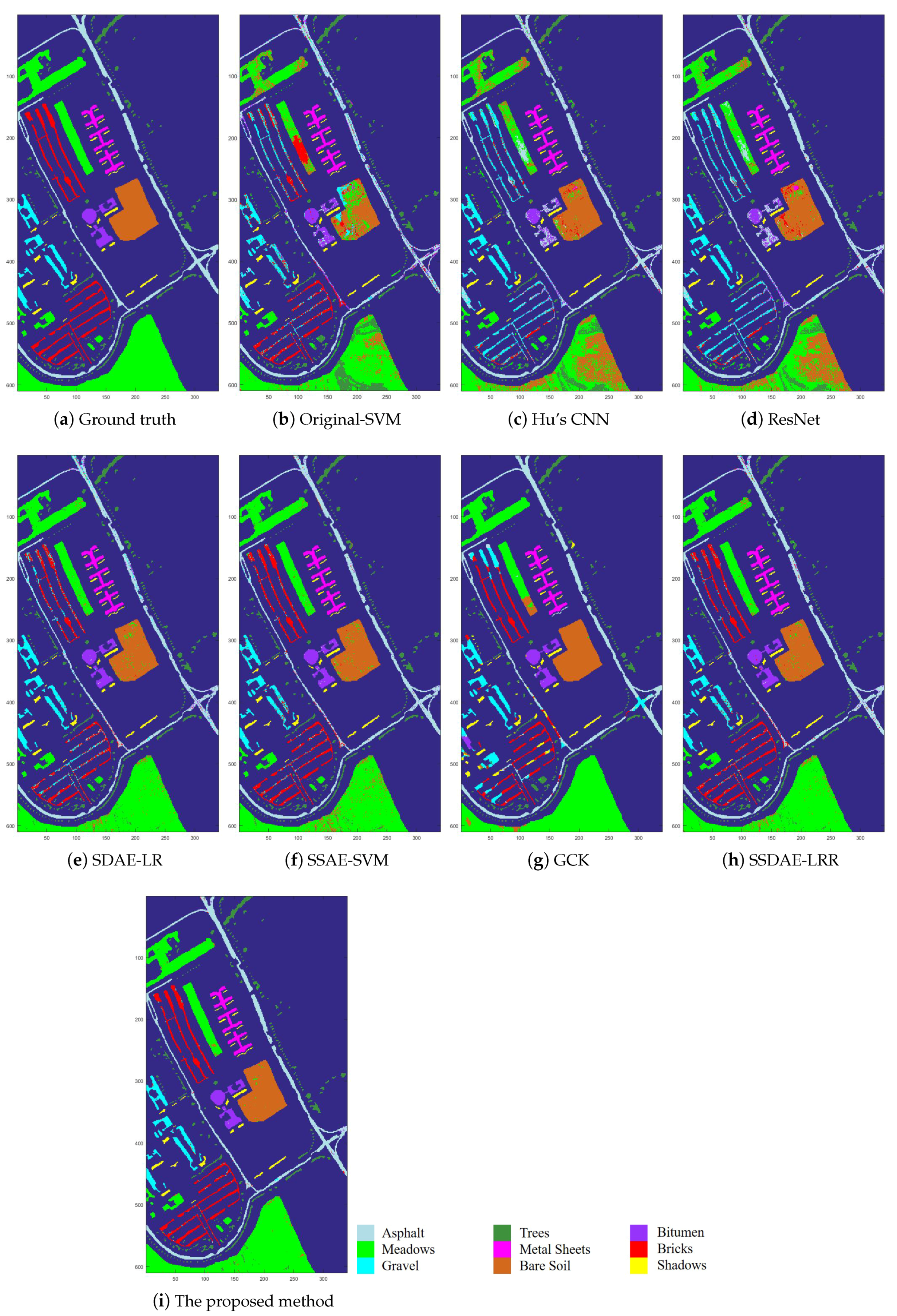
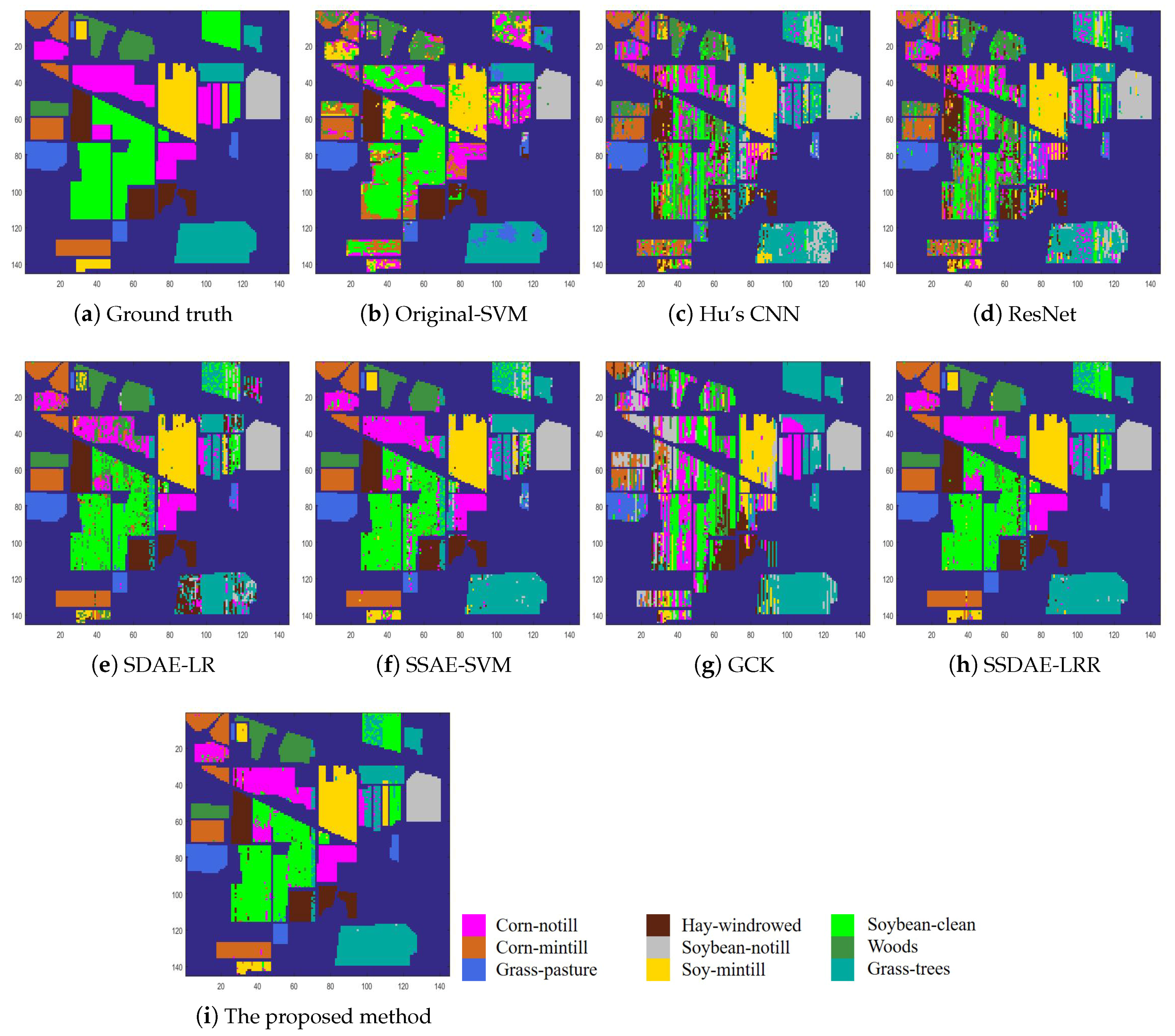
In order to further illustrate the superiority of the proposed method, we show the visual classification maps for all methods in Figure 8, Figure 9, Figure 10 and Figure 11. It can be seen that the proposed method shows more homogeneous results in each class than other comparison methods. This is because the proposed method depicts the intra-class similarity and inter-class dissimilarity among all samples well, with the robust classifier, while most of the comparison methods consider each unlabelled sample independently.

According to the results above, we can conclude that the proposed method outperformed the other 7 state-of-the-art comparison methods.

4.5. Effectiveness Verification

In this part, we conduct extensive experiments to validate the effectiveness of the proposed method in three respects. To verify the effectiveness of the deep spatial-spectral feature, we show the experiments of the proposed method and its three deep spatial-spectral feature-based variants in Section 4.5.1; to demonstrate the effectiveness of the robust classifier, the details of the proposed method compared with its three variants based on the robust classifier are given in Section 4.5.2; in Section 4.5.3, the robustness to limited labelled samples is provided.

4.5.1. Effectiveness of the Deep Spatial-Spectral Feature

To demonstrate the effectiveness of the proposed deep spatial-spectral feature (i.e., segmented stacked denoising auto-encoder-based spatial-spectral feature), we compare the proposed method with its three variants, namely Hu’s CNN-LRR, SDAE-LRR, and SSDAE-LRR. Similar to the proposed method, the low-rank representation based classifier (LRR) is adopted by those three variants. In contrast, Hu’s CNN-LRR adopts the supervised learned feature in comparison to Hu’s CNN, SDAE-LRR employs the feature learned by SDAE without segmentation and spatial-spectral setting, while SSDAE-LRR utilizes the feature learned by segmented SDAE without spatial-spectral setting.

With the same experimental setting as Section 4.2, the comparison results of all these methods on two datasets are provided in Table 1 and Table 2. It can be seen that the proposed method outperformed all the other variants in all cases. For example, on the Pavia University dataset, the proposed method outperformed those variants by at least 2.93% in OA, 2.51% in AA, and 2.80% in KAPPA. The superiority over Hu’s CNN-LRR demonstrates that the proposed deep spatial-spectral feature performed even better than the supervised learned feature. The superiority over SSDAE-LRR verifies that the spatial-spectral setting can further improve the representative capacity of HSI. The superiority of SSDAE-LRR over SDAE-LRR illustrates the effectiveness of the band segmentation, which is similar to the conclusion in [21].

In general, the proposed deep spatial-spectral feature is effective for HSI classification.

4.5.2. Effectiveness of the Robust Classifier

To verify the effectiveness of the low-rank representation based classifier (LRR), we compare the proposed method with three variants, including SSDAESS-SVM, SSDAESS-LR and SSDAESS-OMP. For fair comparison, these three variants employ the same segmented SDAE spatial-spectral feature (denoted as SSDAESS) to characterize the unlabelled samples. The only difference from the proposed method is that they adopt different classifiers. In particular, SSDAESS-SVM and SSDAESS-LR adopt the SVM and LR as the classifiers, respectively. In contrast to those two statistical learning-based classifiers, SSDAESS-OMP adopts the sparse representation based classifier, which is implemented by the classical sparse coding method, orthogonal matching pursuit (OMP).

Under the same experimental settings as Section 4.2, the comparison results on two datasets are summarized in

Table 7. Classification accuracy (%) of the proposed method and its three variants with different classifiers on two datasets.

Method	Pavia University			Indian Pines
	AA	OA	KAPPA	AA	OA	KAPPA
SSDAESS-SVM	$98.83\pm 0.03$	$98.36\pm 0.20$	$98.32\pm 0.21$	$94.32\pm 0.11$	$90.88\pm 0.15$	$90.73\pm 0.15$
SSDAESS-LR	$97.59\pm 0.24$	$98.30\pm 0.14$	$98.26\pm 0.23$	$94.22\pm 0.51$	$90.70\pm 0.36$	$90.55\pm 0.35$
SSDAESS-OMP	$98.84\pm 0.05$	$98.38\pm 0.17$	$98.35\pm 0.18$	$94.37\pm 0.09$	$90.96\pm 0.15$	$90.82\pm 0.15$
the proposed method	$\mathbf{99.32}\pm \mathbf{0.45}$	$\mathbf{98.84}\pm \mathbf{0.44}$	$\mathbf{98.81}\pm \mathbf{0.45}$	$\mathbf{95.20}\pm \mathbf{0.12}$	$\mathbf{92.16}\pm \mathbf{0.15}$	$\mathbf{92.03}\pm \mathbf{0.16}$

. It can be seen that the proposed method obviously outperformed these three variants in all cases. Taking the Indian Pines dataset as an example, the proposed method surpassed these variants by at least 0.83% in AA, 1.20% in OA, and 1.21% in KAPPA. With the exception of the supervision provided by the labelled samples, SSDAESS-OMP also considers the similarity between the labelled samples and the unlabelled one which belong to the same class; because of this, it performed better than SSDAESS-SVM and SSDAESS-LR. However, SSDAESS-OMP considers each unlabelled sample independently; viz., it fails to utilize the crucial intra-class similarity as well as the inter-class dissimilarity among those unlabelled samples as the proposed method, which limits its performance.

The experimental results above demonstrate that the proposed robust classifier is effective for HSI classification.

4.5.3. Robustness to Llimited Labelled Samples

Finally, to further demonstrate the potential of the proposed method in dealing with limited labelled samples, we compare the proposed method with seven state-of-the-art methods (namely SSDAE-LRR, RBF-SVM, BP [27], ResNet, GCK, SDAE-LR, and SSAE-SVM) on two datasets with different numbers of labelled samples.

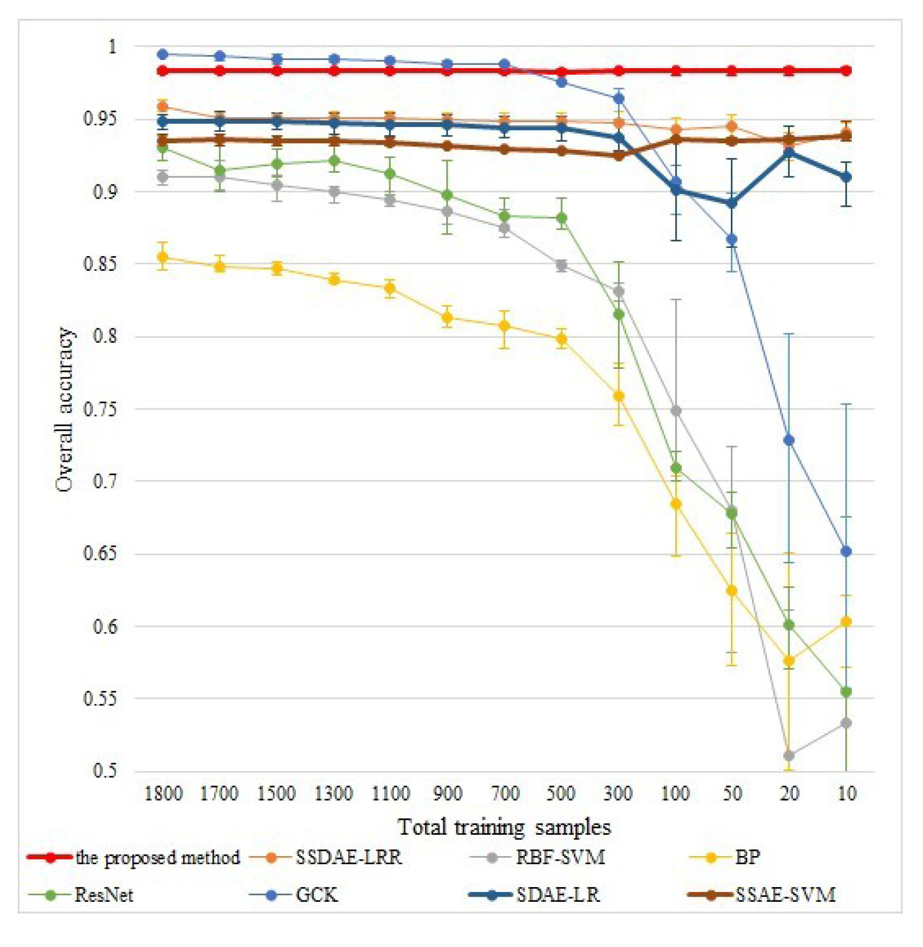
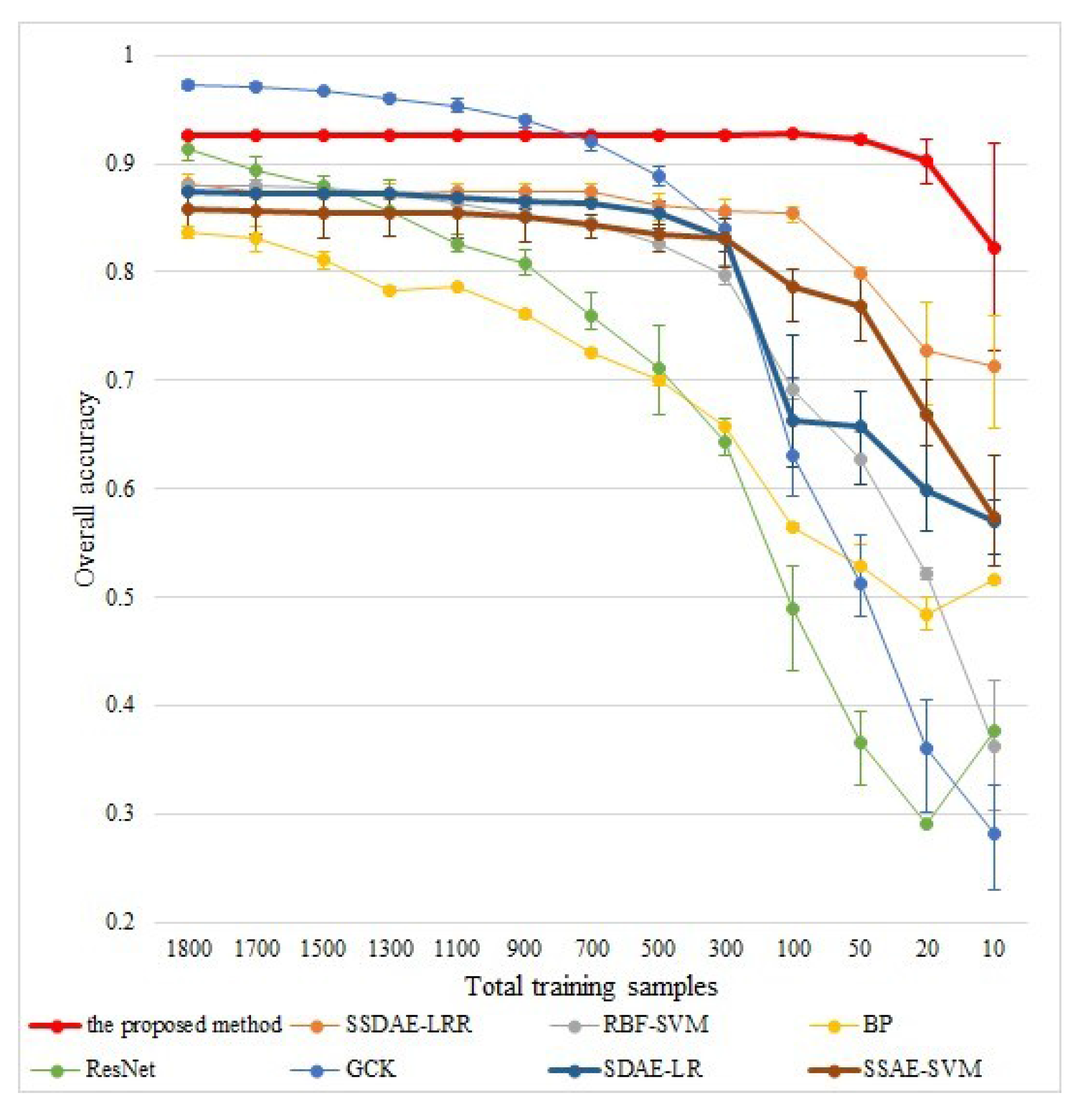
When the total number of the labelled samples ranges from 10 to 1800 (we balanced the number of samples in each class as much as possible), the classification results for all methods on two datasets are shown in Figure 12 and Figure 13. In Figure 12, we can find that when the total labelled samples were more than 900 (samples per class were more than 100), the classification accuracy for all methods was still over 81%, and the proposed method was comparable to GCK. When the total number of labelled samples decreased below 900 (samples per class were less than 100), the performances of RBF-SVM, BP, ResNet, and GCK dropped sharply. Similar phenomena can also be observed in Figure 13. This demonstrates that both supervised-learned features and unsupervised-learned shallow features are sensitive to the amount of labelled samples. In contrast, the proposed method preserved its performance well, even when the total number of labelled samples was 10 (one sample per class), as shown in Figure 12; on the Pavia University dataset, the overall accuracy was 98.40%, and the performances of SSDAE-LRR, SDAE-LR, and SSAE-SVM dropped slightly. These demonstrate that both the unsupervised-learned deep features performed robustly to the limited labelled sample; although SDAE-LR is an supervised method, it can utilise more unlabelled information in the training phase. Since the proposed SSDAE feature further considers the spatial information as well as embedding it into a robust classifier, the proposed method outperformed SSDAE-LRR in all cases. Moreover, the superiority was increased when the total number of labelled samples dropped, especially in Figure 13.

Therefore, we can conclude that the proposed method is effective for HSI classification with limited labelled samples.

5. Discussion

In this paper, a low-rank representation based HSI classification framework is proposed. The experimental results above demonstrate the effectiveness of the proposed method, especially when the labelled samples are limited.

According to the results of the experiments, it can be seen that when the number of labelled samples is fixed as in Table 3 and Table 4, the proposed method not only obviously surpassed SVM which with shallow structure, but also even outperforms the state-of-the-art supervised feature learning methods with deep neural networks (e.g., Hu’s CNN and ResNet). The reason for this comes from two aspects.

On one hand, the proposed method adopts the SSDAE framework to allow features to be learned unsupervised with a deep hierarchical structure, which enables the resulting features to be much more representative than the shallow features which were heuristically learned by those unsupervised feature learning-based methods. Although Hu’s CNN and ResNet also adopt the deeply learned features, their supervised feature learning scheme is prone to being trapped in local minima (i.e., over-fitting), especially when the labelled samples are limited. Meanwhile, the proposed unsupervised deep feature learning scheme has sufficient unlabelled samples for training.

On the other hand, all of the methods compared herein establish their classifiers based only on the supervision provided by the labelled samples, while the proposed method incorporates the supervision as well as the crucial unsupervision (i.e., inter-class similarity and inter-class dissimilarity) provided by unlabelled samples into a robust classifier.

In addition, the proposed method obviously outperformed two sets of variants—one set with different features as in

Table 8. Classification accuracy (%) of the proposed method and its three variants with different features on two datasets.

Method	Pavia University			Indian Pines
	AA	OA	KAPPA	AA	OA	KAPPA
Hu’s CNN-LRR	$93.57\pm 0.34$	$93.87\pm 0.61$	$90.26\pm 1.12$	$92.81\pm 0.56$	$90.17\pm 0.59$	$87.95\pm 0.43$
SDAE-LRR	$96.39\pm 0.15$	$95.39\pm 0.12$	$95.28\pm 0.14$	$92.21\pm 0.68$	$87.63\pm 1.38$	$87.43\pm 1.40$
SSDAE-LRR	$96.81\pm 0.21$	$95.91\pm 0.32$	$96.01\pm 0.18$	$92.78\pm 0.73$	$88.19\pm 1.15$	$88.01\pm 0.87$
the proposed method	$\mathbf{99.32}\pm \mathbf{0.45}$	$\mathbf{98.84}\pm \mathbf{0.44}$	$\mathbf{98.81}\pm \mathbf{0.45}$	$\mathbf{95.20}\pm \mathbf{0.12}$	$\mathbf{92.16}\pm \mathbf{0.15}$	$\mathbf{92.03}\pm \mathbf{0.16}$

, and the other with different classifiers as in Table 7. This demonstrates that both the proposed deep unsupervised feature learning scheme and the robust classification are crucial for HSIs classification. Finally, with a variable number of labelled samples, the stable superiority of the proposed method over the compared methods demonstrates the effectiveness of the proposed method in addressing HSIs classification with limited labelled samples.

6. Conclusions

In this study, we present a novel low-rank representation based HSI classification framework which obviously improves the classification accuracy—especially when the number of labelled samples is limited. On one hand, to better characterize each pixel in the HSI, we propose the unsupervised learning of the deep spatial-spectral feature for each pixel with the segmented SDAE. On the other hand, we developed a robust classifier which simultaneously exploits the supervision provided by labelled samples and the unsupervised correlation (i.e., intra-class similarity as well as inter-class dissimilarity) among unlabelled samples. Both of these advantages benefit the proposed framework in improving classification performance. Extensive experimental results demonstrate the superiority of the proposed framework over several state-of-the-art methods.

In this work, the unsupervised learning scheme and the robust classification are modelled separately. In the future, we can integrate these two modules into a two-branch neural network. With the joint end-to-end training, the feature learning and the classification can be refined by each other, and thus further improvements in HSI classification can be expected.