Data Field-Based K-Means Clustering for Spatio-Temporal Seismicity Analysis and Hazard Assessment
by
 and
and
Xueyi Shang
1, 
Xibing Li
1,*, 
Antonio Morales-Esteban
2, 
Gualberto Asencio-Cortés
3 and
Zewei Wang
4 1
School of Resources and Safety Engineering, Central South University, Changsha 410083, China
2
Department of Building Structures and Geotechnical Engineering, University of Seville, 41004 Sevilla, Spain
3
Department of Computer Science, Pablo de Olavide University of Seville, 41013 Sevilla, Spain
4
School of Earthquake Sciences and Engineering, Sysu, Sun Yat-Sen University, Guangzhou 510275, China
*
Author to whom correspondence should be addressed.
Remote Sens. 2018, 10(3), 461; https://doi.org/10.3390/rs10030461
Submission received: 22 January 2018
/
Revised: 3 March 2018
/
Accepted: 14 March 2018
/
Published: 15 March 2018
(This article belongs to the Special Issue Advanced Machine Learning and Big Data Analytics in Remote Sensing for Natural Hazards Management)
Abstract
:Microseismic sensing taking advantage of sensors can remotely monitor seismic activities and evaluate seismic hazard. Compared with experts’ seismic event clusters, clustering algorithms are more objective, and they can handle many seismic events. Many methods have been proposed for seismic event clustering and the K-means clustering technique has become the most famous one. However, K-means can be affected by noise events (large location error events) and initial cluster centers. In this paper, a data field-based K-means clustering methodology is proposed for seismicity analysis. The application of synthetic data and real seismic data have shown its effectiveness in removing noise events as well as finding good initial cluster centers. Furthermore, we introduced the time parameter into the K-means clustering process and applied it to seismic events obtained from the Chinese Yongshaba mine. The results show that the time-event location distance and data field-based K-means clustering can divide seismic events by both space and time, which provides a new insight for seismicity analysis compared with event location distance and data field-based K-means clustering. The Krzanowski-Lai (KL) index obtains a maximum value when the number of clusters is five: the energy index (EI) shows that clusters C1, C3 and C5 have very critical periods. In conclusion, the time-event location distance, and the data field-based K-means clustering can provide an effective methodology for seismicity analysis and hazard assessment. In addition, further study can be done by considering time-event location-magnitude distances.

1. Introduction
Seismic event clustering provides an effective way to understand the underlying information (such as geological structure interpretation and seismic hazard assessment; a detailed use of seismic event clusters is shown in Section 2) of microseismic events [1,2]. This task can be conducted by experts, following a two-step clustering process: selecting the time period concerned and dividing seismic events into clusters visually by event locations. However, experts’ clusters are subjective, non-quantitative and have trouble handling a large number of seismic events [3]. Motivated by this, various clustering algorithms have been proposed for seismicity analysis (e.g., K-means cluster, hierarchical clustering, and self-organizing map (SOM)), among which K-means clustering technique is the most well-known one. Yet, K-means cannot remove noise events (which have relatively large event location errors) and it uses random initial cluster centers (which have a large influence on cluster results). In addition, no K-means clustering-based methodologies previously applied to this problem have considered time parameters. In fact, seismic events are not only related to the event location but also to the event time [1].
In this work, a data field-based K-means clustering methodology has been proposed for spatio-temporal seismicity analysis. This method uses a data field-based threshold value to remove noises and a new distance-based method to select good initial cluster centers for K-means. Furthermore, we introduced the time-event location distance into the K-means clustering process, which provides a spatio-temporal insight into the seismicity analysis. The real seismic data application shows its effectiveness in seismic hazard assessment. In addition, we compared its performance with classical K-means cluster, hierarchical clustering and SOM clustering. The rest of this paper is organized as follows. In Section 2, related works about seismic event clustering are introduced. Then, in Section 3, the data field theory is briefly illustrated, and the data field-based algorithm is proposed to better select K-means initial cluster centers. In Section 4, the proposed data field-based K-means clustering was applied to 1210 microseismic events obtained from the Chinese Yongshaba mine and the energy index (EI) is selected to assess seismic hazard for the clustering zones. The application detail effect and comparisons with classical K-means cluster, hierarchical clustering and SOM clustering are discussed in Section 5. Finally, brief conclusions of the work and future work are shown in Section 6.
2. Related Works
Seismic event clustering using clustering algorithms has been studied since the 1990s, and the K-means clustering algorithm has become the most famous one. K-means is a hard-partitioning algorithm proposed by Hartigan and Wong [4]. It starts with K randomly selected initial cluster centers and uses an iterative process until no data point changes the cluster assignations. Burton et al. [5] and Weatherill and Burton [6,7] proposed a line-source K-means clustering technique to better identify initial cluster centers and they applied it to capture the seismic spatial variation, interpret the fault type and analyze the probabilistic seismic hazard in the Java island and the Aegean region. Ramdani et al. [8] took advantage of the final K-Means cluster centers to find subduction evidence beneath the Gibraltar Arc and the Andean regions. Rehman et al. [9] utilizes the K-means algorithm to identify the earthquake spatial differences and estimate seismic hazard and risk in Pakistan. Morales-Esteban et al. [10] proposed an efficient adaptive Mahalanobis-based K-means algorithm and this has been applied to study the seismic catalogues of Croatia and the Iberian Peninsula. Shang et al. [11] proposed a Krzanowski–Lai and Silhouette combined index to select the optimum number of clusters for K-means and they interpreted the geological structure in the Chinese Yongshaba mine. The K-means cluster is useful for a large dataset cluster, and some studies have been done to reduce the effect of initial cluster centers. Nevertheless, the above-mentioned methods have not considered the time parameter and the effect of noise events.
Hierarchical clustering is also widely used in seismicity partitioning. It is based on the core idea that an event is more related to a near one than to a far event, and it connects events into clusters based on a preset distance. Hierarchical clustering does not need to set a cluster number (just select a preset distance) and it can cluster events into different shapes. Wardlaw et al. [12], Frohlich and Davis [13], Davis and Frohlich [14], Hudyma and Potvin [15], and Hashemi and Mehdizadeh [16] used hierarchical clustering (single-link analysis) to study earthquake catalogues and seismic activities. Notwithstanding, hierarchical clustering has a tendency to form seismic events into linear groups [13] and there may be many clusters that just have few events (see the discussion).
Another commonly used seismic event cluster method is the SOM [17]. The SOM converts high dimension input space into a low-dimension (typically two-dimensional), which has a very good visualizing image. Zamani and Hashemi [3] compared hierarchical clustering (Ward’s method) and SOM clustering with an application to seismic zoning in Iran. Moreover, Zamani et al. [18] applied the SOM for clustering tectonic zoning in Iran. The same method was tested in Zamani et al. [19], in which Wilk’s Lambda criterion was used to select an optimum number of clusters. Mojarab et al. [20] discussed the effect of SOM input parameters and proposed a combined model to select a cluster number for Iran seismicity analysis. Besheli et al. [21] performed a K-means clustering along with a SOM on an Iranian foreshock database and they found a foreshock zone which has a very close relation with large earthquakes. Nonetheless, research results [11,22] have shown that the SOM clustering may only be valid for high seismic activity areas, while for low seismic activity zones it may have bad cluster results. Furthermore, the SOM clustering may have discontinuous zones, which makes it hard to interpret cluster results [11,22].
Some other cluster methods are proposed for seismicity analysis. Ansari et al. [23], Benitez et al. [24] and Monem and Hashemy [25] used fuzzy clusters, including Gath-Geva clustering, proposed Gath-Geva clustering, fuzzy c-means clustering and Gustafson-Kessel (GK) clustering, to study seismic spatial pattern recognition in Iran, south-west Colombia and the Ghazvin canal irrigation network. The fuzzy clusters can be used for a large dataset cluster; however, its cluster result is sensitive to the initial cluster centers. Mukhopadhyay et al. [26] used a point density clustering to gain insight into subduction kinematics and seismic potentiality. Georgoulas et al. [1] modified a density-based clustering (DBC) algorithm and then used a hierarchical agglomerative scheme for seismic clustering. Nanda and Panda [27] proposed two DBC algorithms and compared them with the DBSCAN (density-based spatial clustering of applications with noise). DBC can remove noise events, yet when the density varies much, it usually obtains bad cluster results. Martínez-Álvarez et al. [22] used a TriGen-based clustering algorithm [28,29] for seismic zoning in the Iberian Peninsula. A comparison of using different seismic clusters can be found in [11,30,31].
Only a few of the above investigations have considered the time factor. Nevertheless, the time parameter can play an important role in seismic event clusters. The commonly used clustering techniques considering a time parameter are the time-event location and time-event location-magnitude distance-based clusters. Frohlich and Davis [13] and Davis and Frohlich [14] suggested equalizing the time and space intervals using a scaling constant and introduced the time-event location distance by , where dij and tij are the event location distance and time interval respectively. Then, they used the hierarchical cluster for seismic event clusters. Baiesi and Paczuski [32] defined the time–event location-magnitude distance between event i and j by , where is the fractal dimension of epicenters, b is the Gutenberg–Richter b-value and is the event magnitude. A single link method was used in this work for the seismic event cluster. Zaliapin et al. [33] and Zaliapin and Ben-Zion [34,35,36,37,38] defined the by magnitude-normalized time component and space component ( and , where q + p = 1). Event j is clustered to the main event i if it satisfies the following conditions: , and . It is clear that no time parameter has been applied in K-means clustering. In this work, we just introduced the time-event location distance into a K-means clustering algorithm. Further study can be done by using a time-event location-magnitude distance.
3. Preliminary Studies and the Proposed Method
In first place, to prove the limitations of the K-means technique, a brief study with synthetic data was performed in Section 3.1. Next, the data field theory is introduced in Section 3.2. Then, the data field-based K-means clustering procedure is proposed in Section 3.3. Finally, an application test of data field-based K-means clustering is shown in Section 3.4.
3.1. K-Means Clustering Preliminary Study
The classical K-means algorithm is based on the following steps: take a dataset of points (x1, x2, …, xn), randomly select K points from the data set as the initial cluster centers and allocate each point xi to the nearest center point. Then, it calculates the mean of each parameter respectively for each group to make up a set of new updated cluster centers. This procedure is repeated until no points change their cluster or the number of iterations reaches a preset maximum.
The most widely used distance is the Euclidean function and this was chosen for this work. The Euclidean distance between event xi and xj is defined in Equation (1). Then, the mean of the widely used clustering criterion-sum of Euclidean distance (SED) is used to evaluate the cluster performance. We called this the MSED index. (The number of undenoised and denoised events is different, so we used the MSED instead of the SED to evaluate the clustering performance). MSED is defined in Equation (2), the smaller the MSED index of clusters the better the clustering results.
where is the distance between event xi and xj, p is the dimension of the parameters, Ck is the kth cluster, K is the cluster number, mk is the cluster center of Ck, and n is the number of cluster events.
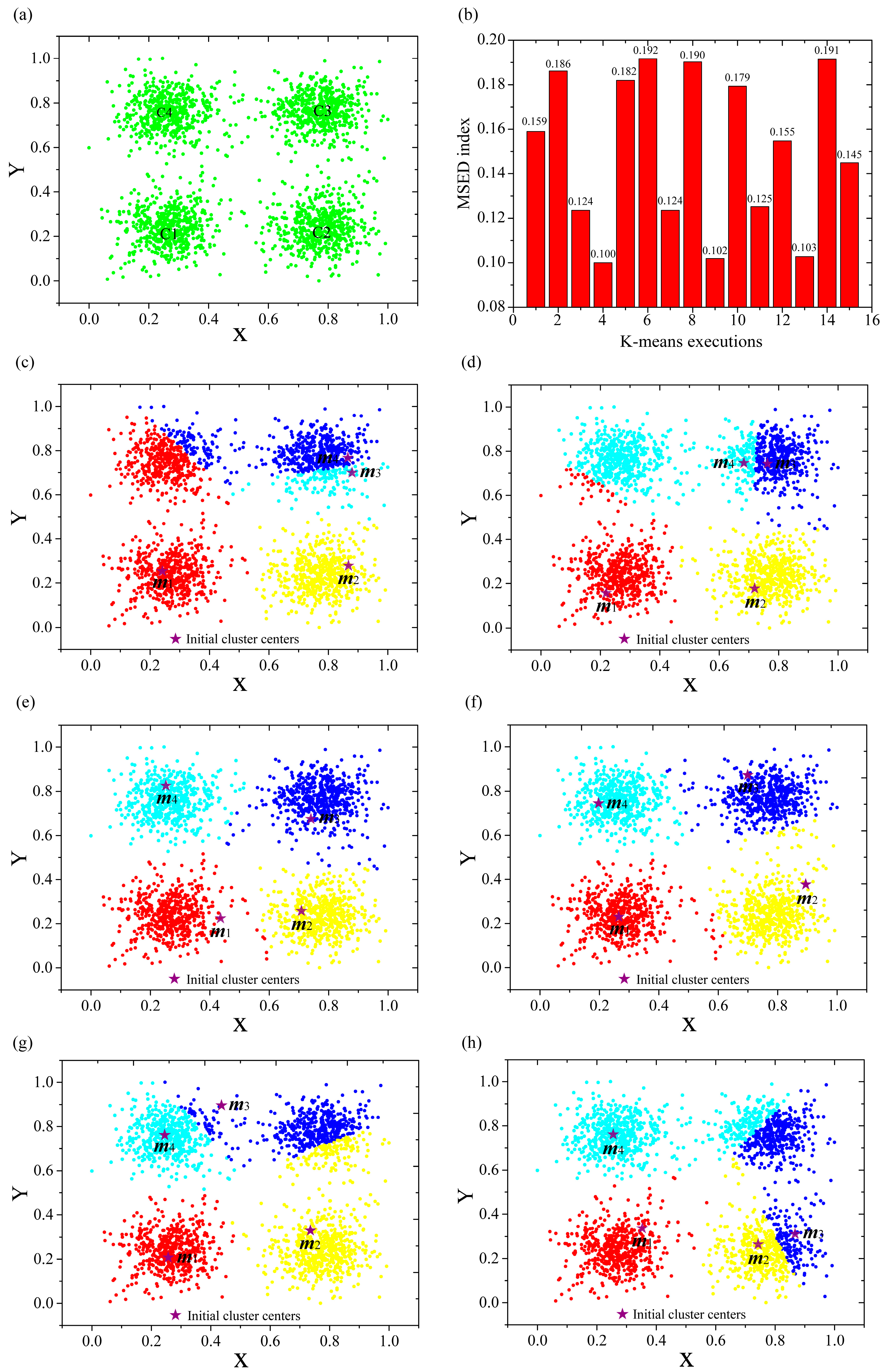
From the principle of K-means clustering, we know that the algorithm may be affected by the initial cluster centers. To prove this issue, a synthetic two-dimension dataset with four well-differenced clusters is used to test the effect of K-means initial cluster centers (Figure 1a). The algorithm was tested 15 times by using randomly generated initial cluster centers (using K = 4 for all the experiments) and their MSED indexes are shown in Figure 1b. It is clear that the K-means clustering can be heavily affected by the initial cluster centers: the MSED index varies from 0.100 to 0.192. The K-means clustering results for six typical MSED values are shown in Figure 1c–h. It is clearly seen that for high MSED values, quite a lot of close events are in different clusters (Figure 1c,h); for relatively high MSED values, many close events are in different clusters (Figure 1d,g); while for low MSED values, the K-means cluster has good results (Figure 1e,f). In conclusion, the lower the MSED index, the better the clustering result. Therefore, there is a high need to optimize the K-means initial cluster centers. Furthermore, there are some noise events placed in inter-cluster regions, which should be removed before clustering.
3.2. Data Field Theory
Motivated by physical field theory, Wang et al. [39] proposed a data field theory to describe the interaction among a set of events. The potential value (scalar field strength) of event xi in the global data field is defined as:
where is the mass of event xj, K(x) is the unit potential function, represents the distance between event xi and event xj, and is the impact factor.
The is set to 1, for all the j values, and the commonly used function is selected. Then, the potential value in the global data field for event xi can be written as in Equation (4), where was defined by the Euclidean function.
The impact factor controls the interacted distance between events and its value can have a heavy impact on potential values. The relationship between the interacted distance and the potential value of Equation (4) is shown in Figure 2a. It is easy to see that the longer the distance between events the lower the potential value for a same impact factor, and the higher the impact factor the larger the potential value for a same interacted distance. In other words, for a low impact factor, there will be many local maximum potential values; while for a large impact factor, there will be few local maximum potential values. Some research [39,40] has used potential entropy to obtain an optimum impact factor, and the minimum potential entropy corresponds to the optimum impact factor. The potential entropy is defined as in [39]:
where , .
The potential entropy using different impact factors is shown in Figure 2b. The potential entropy has a minimum value when . Then, the potential value is calculated for each event using Equation (4). The contour map of potential value is shown in Figure 2c. It is easy to see that the potential value contour has a good agreement with the dataset density. Potential value may provide a good way for clustering (e.g., Figure 2c): a potential threshold value can be used to divide the dataset into small datasets. Notwithstanding, for an irregular dataset, it is difficult to produce adequate clusters based on a potential threshold value (e.g., Figures 5a and 6). Therefore, instead of using a potential value to cluster seismic events, we just applied potential threshold values to remove noise events and better selected K-means initial cluster centers.
3.3. Data Field-Based K-Means Clustering Procedure
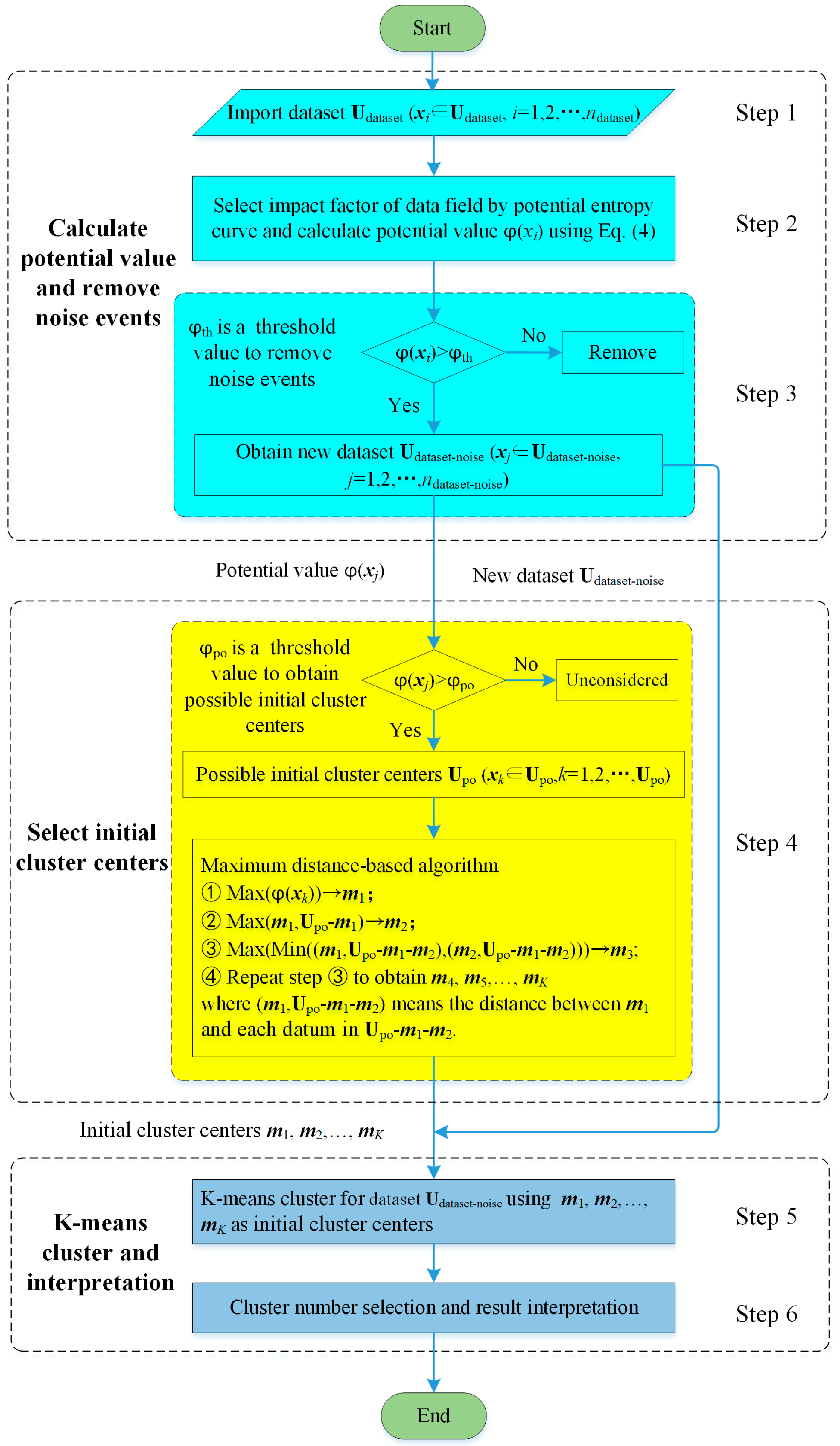
The data field-based K-means clustering takes advantage of the event with high potential value being more likely to be an initial cluster center and that the distance between initial cluster centers should have a larger distance. There is a low event density around the noise events and they have larger distances to most events, which usually implies small potential values. Then, a threshold value can be set to remove noise events. The flow diagram of the data field-based K-means clustering process is shown in Figure 3 containing the following steps:
Step 1: Input dataset Udataset (xi ∈ Udataset, i = 1, 2, …, ndataset, ndataset = n).
Step 2: Select the impact factor of the data field by the impact factor-potential entropy curve calculated by Equation (5) and calculate the potential value ϕ(xi) for each event in Udataset using Equation (4).
Step 3: Remove noise events and obtain a new dataset Udataset-noise (xj ∈ Udataset-noise, j = 1, 2, …, ndataset-noise, ndataset-noise ≤ n): If a potential value is smaller than a predefined threshold value , then its corresponding event is marked as a noise event and it is to be removed from the dataset Udataset. If there are no noise events, then there is no need to do Step 3 or a that is smaller than the minimum potential value can be set to do Step 3. = Min-0.1 is used in this paper for no denoising, where Min-0.1 means the minimum potential value minus 0.1.
Step 4: Select K-means initial cluster centers based on the potential value and a maximum distance-based algorithm.
(4-1) Select possible initial cluster centers Upo (xk ∈ Upo, k = 1, 2, …, npo, npo ≤ n) by choosing events which have potential values larger than a predefined threshold value ;
(4-2) Select K-means initial cluster centers based on a maximum distance-based algorithm. The maximum distance-based algorithm contains the following steps:
(4-2-1) The event which has a maximum potential value in Upo is set to the first initial cluster center m1;
(4-2-2) Calculate the distances between m1 and each point in Upo-m1, and the largest distance corresponding event is set to the second initial cluster center m2;
(4-2-3) Calculate the distances between m1, m2 and each point in Upo-m1-m2, then select the smallest distance to obtain the distance set Vsd. For example, for event xi(xi Upo-m1-m2), there are two distances (m1,xi) and (m2,xi), and the Min((m1,xi), (m2,xi)) is set to . Calculate the smaller distance for each event in Upo-m1-m2, then the smallest distances make up the distance set Vsd. The point with the largest value in Vsd corresponds to the third initial cluster center m3;
(4-2-4) Repeat Step (4-2-3) to obtain m4, m5, …, mK.
Step 5: Perform the K-means clustering for dataset Udataset-noise using the m1, m2, …, mK as the initial cluster centers.
Step 6: Select the optimum number of clusters using the Krzanowski-Lai (KL) index (see Section 4.3.2) and interpret the clustering results.
3.4. Application Test
The relationship between the MSED index and the threshold value for data field-based K-means clustering using undenoised data is shown in Figure 2d, where O1, O2, …., O7 are the first, second, …, and seventh octiles of potential values, respectively. It is clear that the data field-based K-means clustering usually obtains a smaller MSED index than the classical K-means algorithm. This indicates that the data field-based K-means clustering obtains better clusters than those produced by the classical K-means. A larger achieves a lower MSED index in the application test, which can be interpreted as that, for a low , the selected possible initial cluster centers may contain noise events. The noise events are usually far away from the final optimum cluster centers. Although we used a largest distance principle to select the initial cluster centers, the noise events may be selected as initial cluster centers, and this may cause bad cluster results. For a large , some possible initial cluster centers may not be included, and this can cause a bad clustering result. The testing dataset is nearly equal-distributed, which results in similar local maximum potential values. Furthermore, the MSED index of data field-based K-means clustering results with 7.5% data removed is also shown in Figure 2d. The MSED index of the denoised cluster is much smaller than that of the undenoised cluster. For engineering data, we usually obtain many local maximum potential values with relatively large differences. The effect of in seismic event clusters has been discussed in Section 5. The results show that a threshold value between Q1 and the Median obtains a good cluster result (Q1 and Median are the first quartile and second quartile of the potential values, respectively). In this paper, the is set to Q1 for further study. The data field-based K-means cluster result using undenoised data, when = Min-0.1 and = Q1, is shown in Figure 2e. This shows that the data field-based K-means clustering obtains good clusters. Furthermore, the results with 7.5% events removed are shown in Figure 2f. The noise events are well separated and the data field-based K-means clustering obtains good cluster results. Therefore, we found that this clustering methodology can have a good application to seismic event clustering.
4. Application to Seismic Data
4.1. Seismic Dataset Description
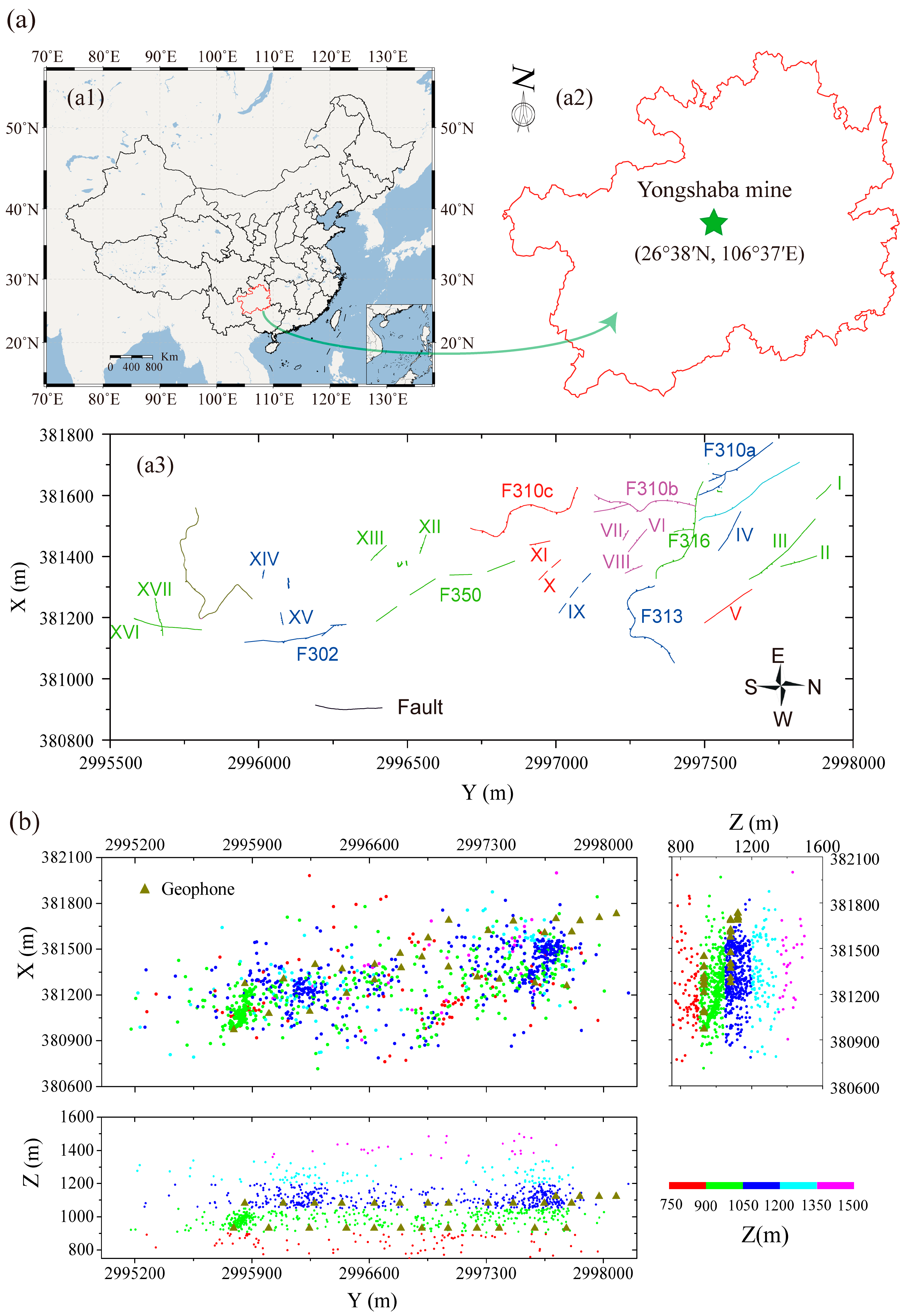
To test the efficiency of the proposed method, we used microseismic events obtained from the Institute of Mine Seismology (IMS) system at the Chinese Yongshaba mine (Figure 4a). The Yongshaba mine is in Guiyang city of Guizhou province (China, 26°38′N, 106°37′E) and has an explored phosphate reserve amount of 40 million tons and an exploitation depth of more than 650 m. The strike and dip angle of the ore body are 280°~293° and 10°~30°, respectively, and the roof of the ore body is very unstable. It uses a multi-stage open stope mining method, which results in many mined-out areas. In addition, there are several main faults (F310, F313, F316, F302 and F309) and many small faults (Figure 4a), which may cause seismic hazards such as rock bursts and large areas of rock instability. Motivated by these concerns, we built the IMS system in the mine. The IMS system contains 28 geophones distributed at the 930 m level (12 geophones), 1080 m level (12 geophones) and 1120 m level (4 geophones). All the geophones have a sampling frequency of 6000 Hz.
We used an absolute-value method (Equation (2) in [41]) based on manual picked P phase arrivals to locate microseismic events. We set the time period from 1 April 2014 to 30 April 2014, then we used a cuboid (380,600 ≤ X ≤ 382,100 (X = East), 2,995,000 ≤ Y ≤ 2,998,200 (Y = North) and 750 ≤ Z ≤ 1600 (Z = Up)) and a moment magnitude ≥ −1.5 to filter events that have very large location errors and small moment magnitudes. Finally, we obtained 1210 microseismic events, which are used as the input dataset (Figure 4b). Generally, the microseismic event locations have a good relationship with the geophone distribution. However, there are some microseismic events which are relatively far away from the geophones. These microseismic events are thought to be badly located and should be removed before clustering.
4.2. Noise Event Removing Process
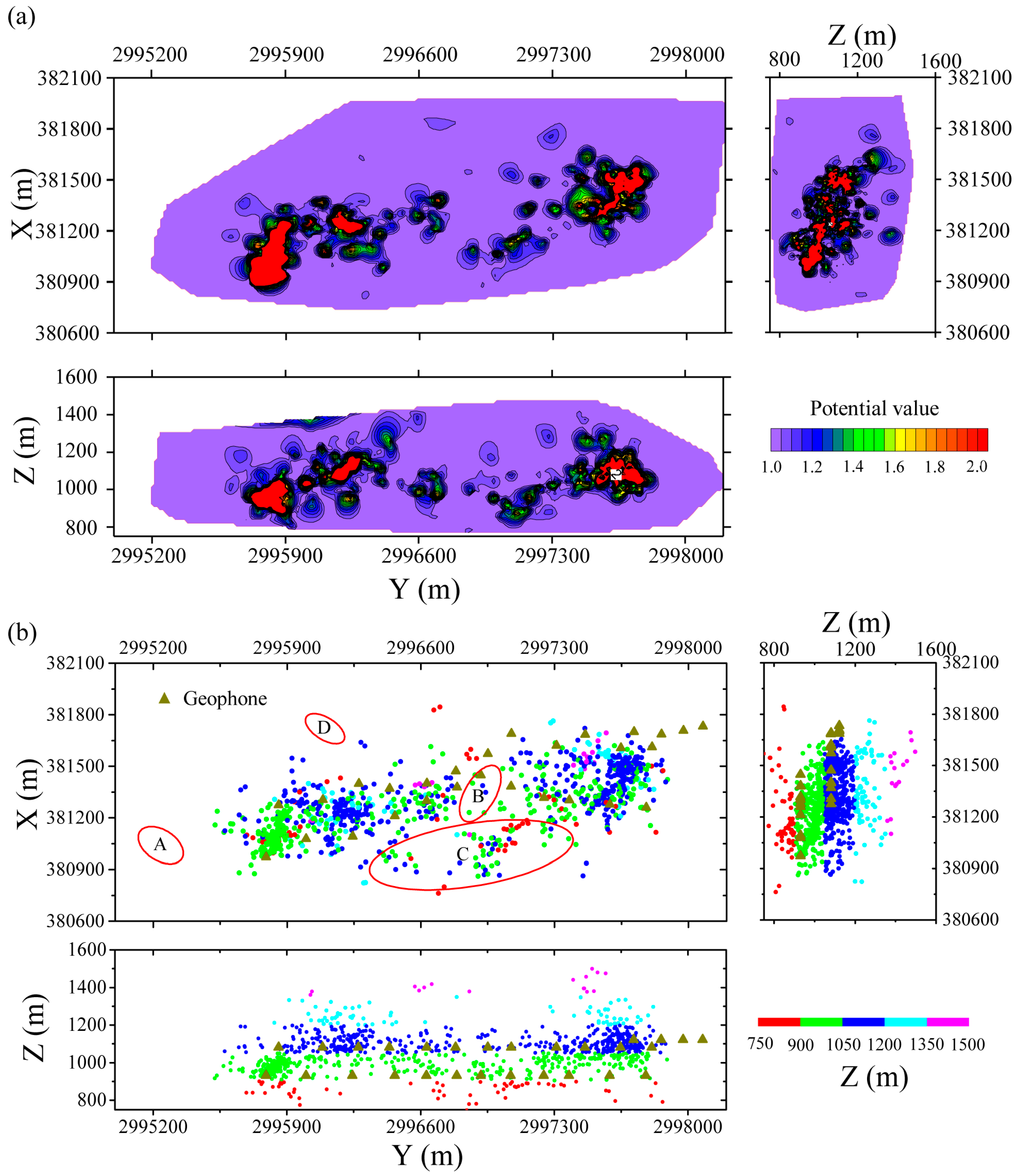
To remove badly located events, the Euclidean distance of the seismic event location parameters (X, Y, Z) is selected to calculate the potential entropy. The microseismic event can have a large location error due to the P phase picking quality, geophone distribution and location algorithm, while the event time can be accurately recorded. After calculating the potential entropy of the data studied, we found that it had a minimum value when σ = 22.00. The contour map of the potential value σ = 22.00 is shown in Figure 5a. It shows that the contour map fits well with the seismic event density. Then, we tried to remove 5%, 7.5%, 10%, 12.5% and 15% of the seismic events which have the lowest potential values. For those five denoising ratios, all the denoised microseismic events have many events in area C. This is due to the approximately linear distributed geophones near area C being able to result in a relatively large location error. For 5% removed seismic events, areas A and D still have few seismic events (Figure S1a); for 7.5% removed seismic events, area D still has few seismic events (Figure S1b); while for 12.5% and 15% removed seismic data, area B removes some useful seismic events (Figure S1c,d). Therefore, microseismic events with 10% of seismic events removed are selected for further study in this paper.
4.3. Seismic Event Clustering Procedure
4.3.1. Time-Event Location Distance-Based Data Field
Most traditional seismic clustering methods only take advantage of seismic event location parameters (X, Y, Z), since the time parameter has a different measurement unit. Frohlich and Davis [13] and Davis and Frohlich [14] suggested equalizing the time and location parameters using the following time-event location distance equation:
where dij (meters) and tij (days) are the event location distance and the time difference between events, and a is the time-event location distance conversion factor. In this paper, a is set to , where dmean and tmean are the mean values of dij and tij (i = 1, 2, …, ndataset-noise; j = 1, 2, …, ndataset-noise), respectively.
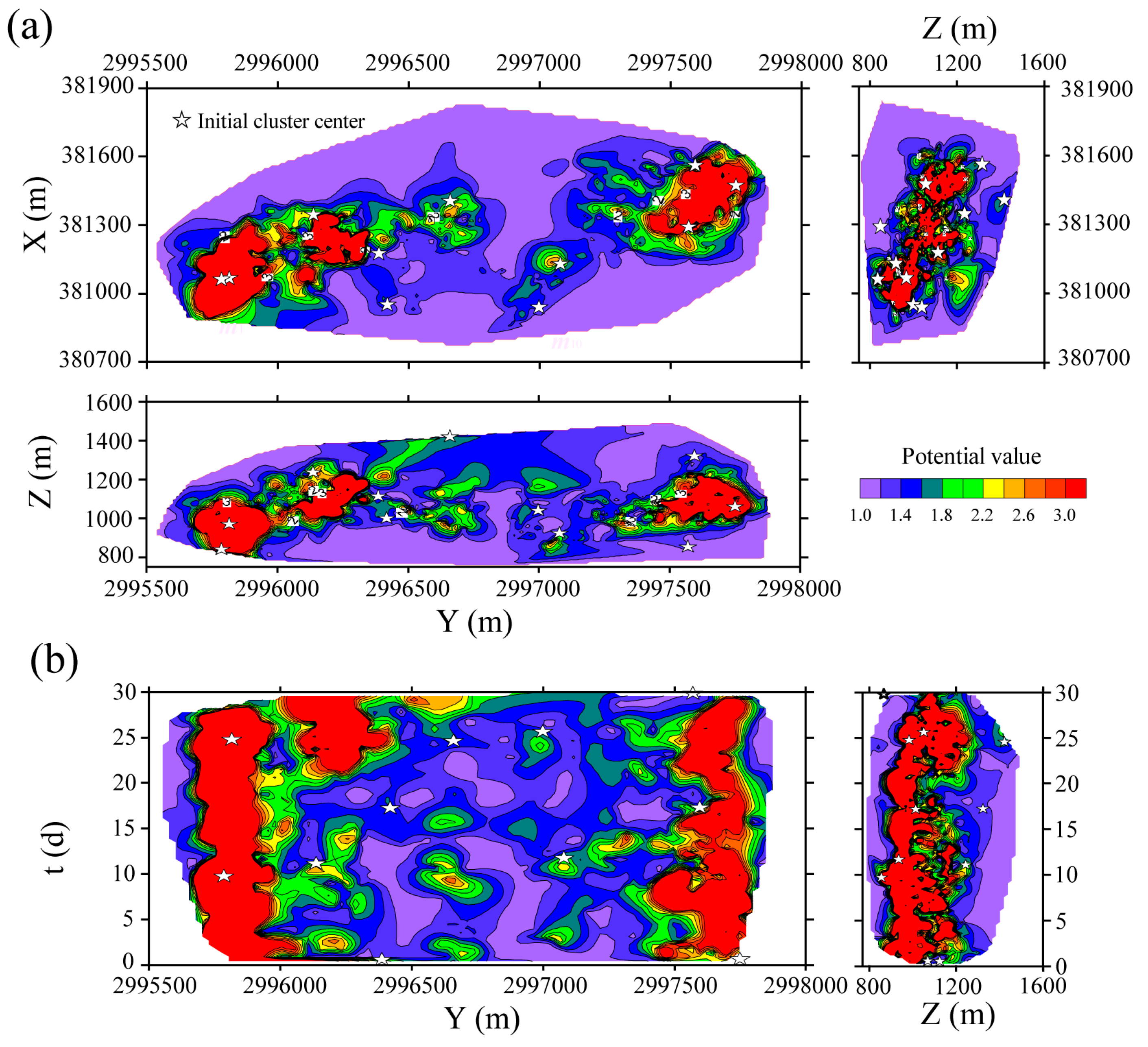
We calculated the dmean and tmean of the denoised microseismic events resulting in 919.31 m and 9.88 d, respectively. Then, the a factor is set to 53.72 m/d by calculating the ratio between dmean and . The potential entropy is calculated by Equation (5) and it has a minimum value when σ = 83.50. The contour map of potential value (σ = 83.50) for the denoised microseismic events taking advantage of the time-event location distance is shown in Figure 6. Then, initial cluster centers were calculated by Step 4 of the data field-based K-means cluster algorithm, and they are also shown in Figure 6. The time-event location distances between the initial cluster centers are listed in Table 1. The initial cluster centers have a good distribution and there are no small time-event location distances between the initial cluster centers, which shows that this algorithm can obtain good initial cluster centers.
4.3.2. Cluster Results
There are many indexes in the literature to select an adequate number of clusters, among which the Silhouette index [43] and Krzanowski-Lai index [44] are the most popular ones. In this paper, the Krzanowski-Lai index is selected. The KL index produces the traces of the within-clusters matrices for two consecutive clusters. The higher the KL index, the better the cluster results. The KL index is defined as in [44].
where , and p is the number of clustering parameters in the dataset. In this paper, the seismic parameters (X, Y, Z, t) are used as the cluster input parameters, which means p is equal to 4. is the sum of all point-to-point distances of the observations within each cluster, summed across all clusters. , where xi and xj are two events in cluster Ck, p is the number of clustering parameters, and K is the cluster number.
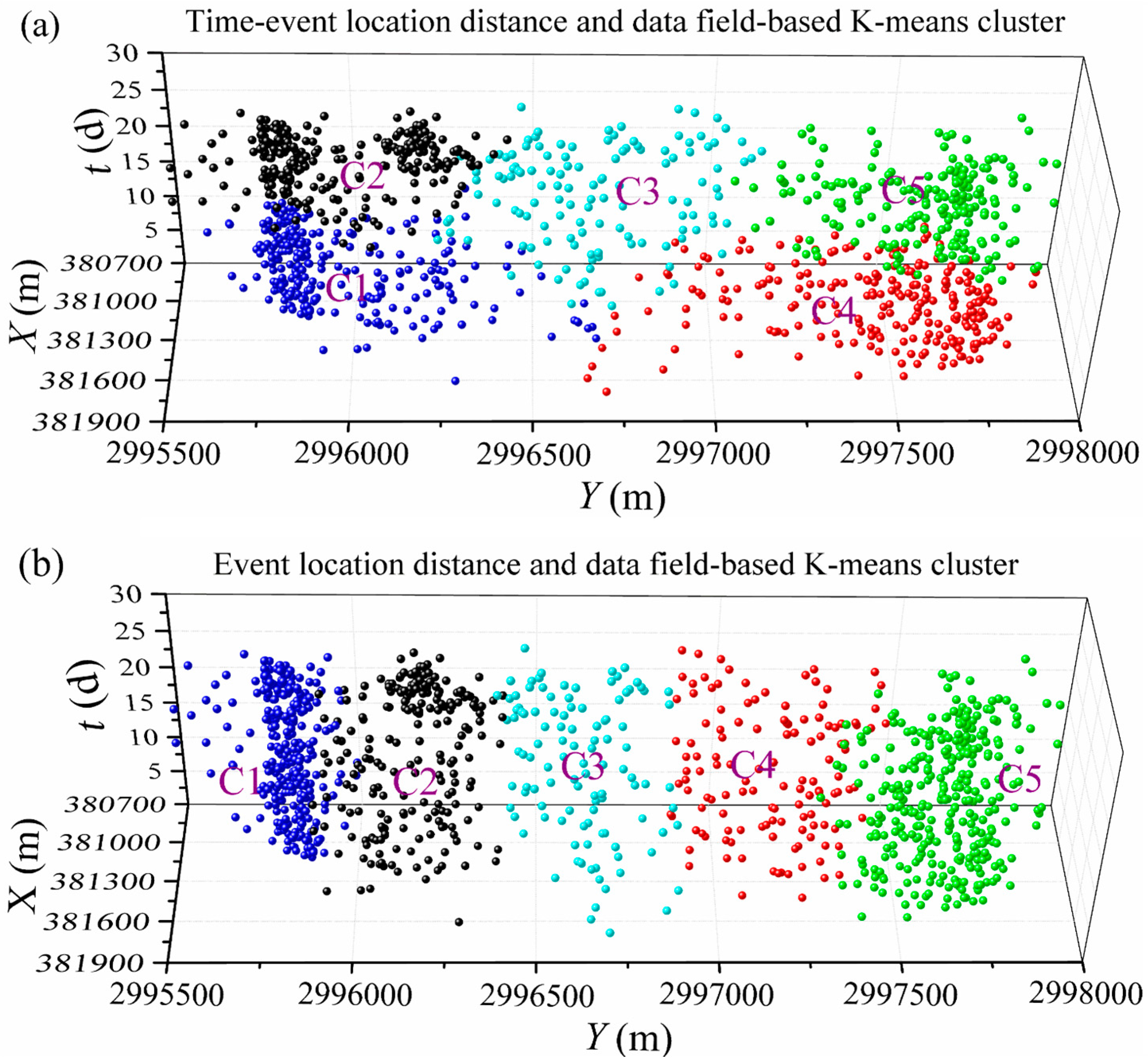
The KL index of the time-event location distance and the data field-based K-means clustering is shown in Figure 7. As this figure indicates that the KL index has a maximum when K = 5, the number of clusters K = 5 is selected for further study. The data field-based K-means clusters using denoised events taking advantage of time-event location parameters (X, Y, Z, t) and event location parameters (X, Y, Z) are drawn in Figure 8a,b, respectively. Figure 8a shows that the time-event location distance-based cluster divides the microseismic events by both space and time, while the location distance-based cluster has few XY overlaps, and the events in each cluster cover almost all the event time (Figure 8b). With the passing of time, the same area events may have large differences, which should be divided (e.g., Figure 9c). Therefore, time-event location distance-based K-means clusters can provide a new insight for seismicity analysis.
4.3.3. Seismicity Analysis
(1) Energy index
The commonly used statistical parameter-energy index (EI) is selected to evaluate microseismic activity. EI is a parameter related to the concentration and accumulation of stress in a rock mass [45], and it is defined as the ratio between the radiated energy and the average energy (expected energy) for a given seismic moment M. An EI > 1 signifies that more energy has been released than expected, while an EI < 1 signifies that less energy has been released than expected. Research has shown that when an EI > 1 the rock mass is accumulating stress, and when the rock mass starts to fail, the EI drops below one [46]. The EI is defined as in [47]:
where is the seismic radiation energy, is the rock density, is the wave propagation speed, is the integral of the squared ground speed, Fc is the radiation pattern parameter: for a P wave Fc is 0.52, while for an S wave Fc is 0.63. is the average energy derived from the logE vs. logM relation for a given moment M, and c and d are the regression constants.
(2) Seismicity analysis of clusters
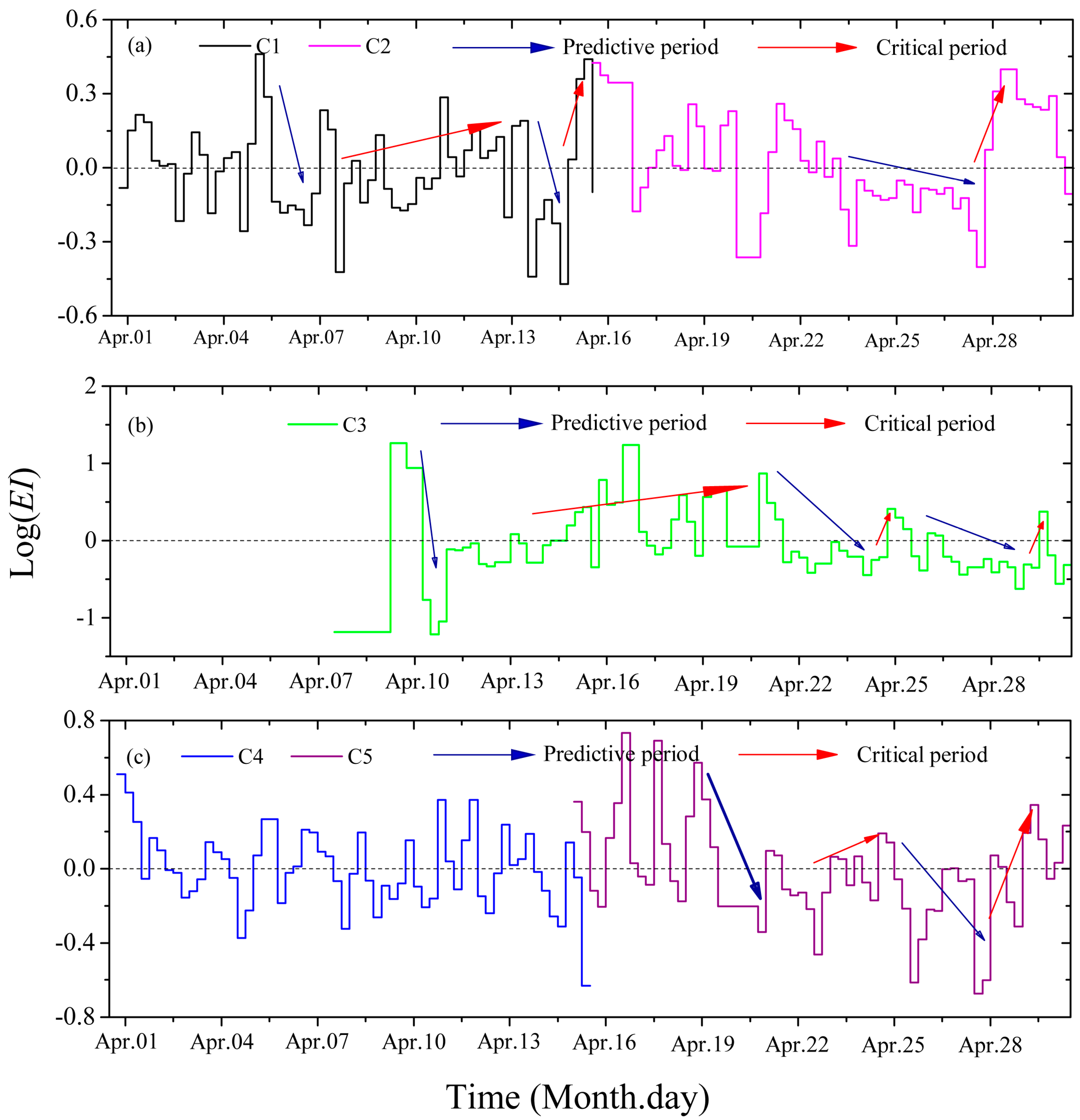
The least squares linear regressions between log(energy) and log(moment) for the five clusters of Figure 8a are shown in Figure S2. Then, we calculated the EI through Equation (8) and the logEI of the five clusters are shown in Figure 9. Some research [48,49] defined the predictive period and critical period from the EI time series: when the EI decreases, this indicates that parts of the rock mass are beginning to have an unstable status. This period could be seen as a strain-softening stage. It is the beginning of potential damage and regarded as a warning indicator. This period is called a predictive period. An increasing EI means that the rock mass is entering an unstable state, and this period is called a critical period. The quicker the EI decreases, the larger the risk of a big microseismic event happening. So, when the EI decreases sharply, we can suggest the miners to be careful in the predictive period and not work in the upcoming critical period in the corresponding cluster area.
For C1, the logEI has a sharp decrease from 5 April to 6 April (a predictive period)–the miners should be careful when mining in this area–and the logEI increases from 7 April to 13 April (a critical period)–the miners should not work in this area on these days. Then, there is a relatively small predictive period (from 13 April to 14 April) and a critical period (15 April). For C2, the logEI slowly decreases from 23 April to 27 April (predictive period), and the miners should be careful on 28 April when mining. For C3, the logEI quickly decreases on 10 April (a predictive period and special attention should be paid) and then the logEI increases from 13 April to 16 April (a critical period and the miners should not work in this area). For C4, the logEI increases and decreases alternately, which means the rock system releases and absorbs energy steadily and there are no predictive periods and critical periods. For C5, there are high logEI from 16 April to 19 April and there is a sharp logEI decreasing from 25 April to 28 April (a predictive period and the miners should be very careful when mining), then the logEI increases from 22 April to 24 April (a critical period and the miners should not work in this area). Though Figure 8a shows that C4 and C5 have a similar location area, C5 has critical periods while C4 has no critical periods, which proves that the time parameter can provide a new insight for seismic clustering analysis. In conclusion, there are very critical periods for C1, C3 and C5 when the miners should not work.
5. Discussion
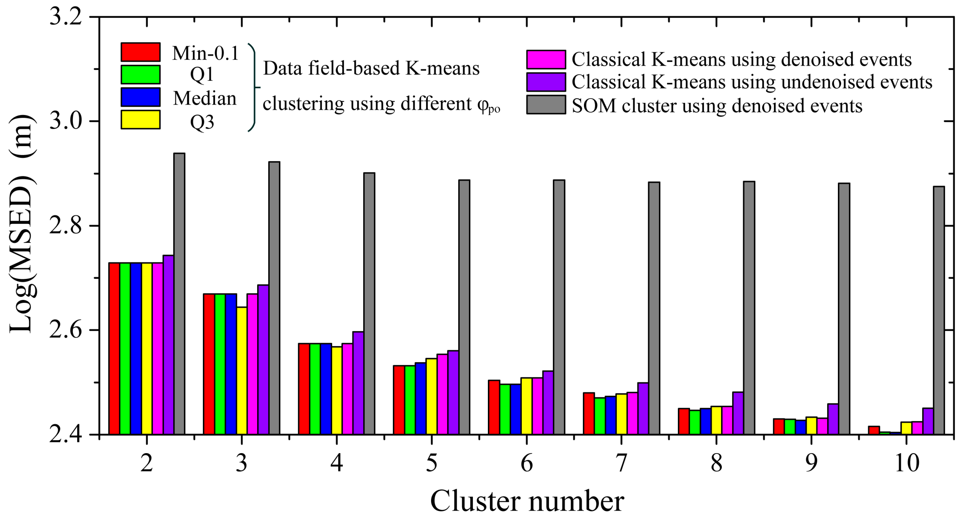
This paper proposed a data field-based K-means clustering methodology to denoise noise events and select initial cluster centers. However, this can be affected by the threshold value , and its performance with respect to classical K-means clustering using denoised and undenoised events should be discussed. In addition, we also chose the commonly used hierarchical clustering and SOM clustering as comparisons. The MSED indexes of time-event location distance and data field-based K-means clustering ( = Min-0.1, Q1, Median and Q3, where Min, Q1, Median and Q3 correspond to the minimum, the first quartile, the second quartile and the third quartile of the potential values, respectively), classical K-means clustering using denoised and undenoised events (randomly selected initial cluster centers) and SOM clustering are drawn in Figure 10. For denoised event clustering, this shows that the MSED index of the data field-based K-means clustering is usually smaller than that of the classical K-means clusters. For a small cluster number (K = 2 and K = 3), the data field-based K-means ( = Min-0.1, Q1 and Median) has a similar MSED index to the classical K-means. This is because the classical K-means clustering has a relatively good global search for a small number of clusters. The data field-based K-means clustering ( = Q3) produces better cluster results than the classical K-means algorithm (K = 3 and K = 4). This is due to the higher potential value event being more likely to be a final cluster center. For a relatively large cluster number (K = 5~7), the data field-based K-means clustering usually improves the classical K-means clustering, which proves the effectiveness of the data field-based algorithm in selecting initial cluster centers. For a large cluster number (K = 8~10), the data field-based K-means clustering ( = Q3) has a result that is nearly as equal/bad as the classical K-means clustering. This is caused by the data field density-based algorithm using a threshold value to select high potential value events. Yet, the low potential value events may have useful initial cluster centers for a large cluster number, which results in the randomly selected initial cluster centers at times having a better cluster result. The data field-based K-means cluster ( = Q1 and = Median) has a good cluster result in general and a threshold value between Q1 and the Median, and a cluster number smaller than 9 is suggested in the data field-based K-means clustering algorithm.
The classical K-means clustering using denoised events usually has a smaller MSED index than that of classical K-means clustering using undenoised events. This is caused by the noise events being relatively far away from most events (Figure 11a). The SOM clustering has a very large MSED index compared with K-means-based clusters (Figure 10). This is due to the SOM clusters sometimes mixing together (Figure 11b). Furthermore, the mixed clusters make it hard to interpret the cluster results. For the hierarchical clustering, we tried different cluster numbers: for a small cluster number, 99% of seismic events are in one cluster; for 100 clusters, 36% and 50% of events are in two clusters; for 200 clusters, 42% and 28% of events are in two clusters; and for 400 clusters, 25% and 12%, 5%, 7% of events are in four clusters. For these numbers of clusters, every other cluster makes up less than 1%. This is brought about by the hierarchical clustering connecting close events together. Although there are some far away events in the seismic data, every event will usually be divided into one cluster or several close events connected into one cluster. Therefore, it is hard to obtain a certain number of clusters which contain a relatively large number of events, and there are many events that will be treated as noises (the clusters with few events). In conclusion, the data field-based K-means clustering can have a good cluster result as well as a good interpretation compared with the above discussed clusters.
6. Conclusions
In this paper, a data field-based K-means clustering method has been proposed for spatio-temporal seismicity analysis. This method takes advantage of a data field-based threshold value to remove noises as well as a new distance-based algorithm to obtain good initial cluster centers for K-means. The method has been tested by its application to microseismic events obtained from the Chinese Yongshaba mine, which considers both a time parameter and location parameters. The KL index shows that the method has the best clustering result when K = 5 and the EI shows that C1, C3 and C5 have very critical periods. C4 and C5 have similar cluster zones. Nevertheless, C4 has no critical periods, which proves that the time-event location distance-based K-means clustering can provide a new way for seismicity analysis compared with event location distance-based K-means clustering. The data field-based K-means clustering usually achieves better cluster results compared with classical K-means clustering when the threshold value is between Q1 and the Median of the potential values and the cluster number is smaller than 9. Comparisons with the classical K-means clustering, hierarchical clustering and SOM clustering show the effectiveness of the proposed clustering method. The potential value-based denoising is very applicable to other datasets, where events need to be divided into clustered and non-clustered events. Also, the potential value can be used to show event density. The proposed maximum distance-based algorithm can also provide good initial cluster centers for some other clusters, such as the FCM cluster. The effectiveness of introducing spatio-temporal distance into K-means shows that it may also be useful in other cluster algorithms. Moreover, further study can be done by introducing time-event location-magnitude distance into the data field-based K-means clustering for seismicity analysis.
Supplementary Materials
The following are available online at https://www.mdpi.com/2072-4292/10/3/461/s1. Figure S1: Seismic event locations with 5%, 7.5%, 12.5% and 15% of data removed. (a) Seismic event locations with 5% of data removed; (b) Seismic event locations with 7.5% of data removed; (c) Seismic event locations with 12.5% of data removed; (d) Seismic event locations with 15% of data removed. Figure S2: Least squares linear regression between log(energy) and log(moment) for the five clusters shown in Figure 8a.
Acknowledgments
The authors gratefully acknowledge the financial support of the National Key Research and Development Program of China (2016YFC0600706). The authors would also like to thank Dong Liu, Yongyong Zhou and Jing Yang for their help.
Author Contributions
Xueyi Shang wrote the paper; Xibing Li provided the original idea and seismic data; A. Morales-Esteban and Gualberto Asencio-Cortés modified the paper and gave some useful suggestions; Zewei Wang wrote part of the program code.
Conflicts of Interest
The authors declare no conflict of interest.
References
- Georgoulas, G.; Konstantaras, A.; Katsifarakis, E.; Stylios, C.D.; Maravelakis, E.; Vachtsevanos, G.J. “Seismic-mass” density-based algorithm for spatio-temporal clustering. Expert Syst. Appl. 2013, 40, 4183–4189. [Google Scholar] [CrossRef]
- Fidani, C.; Battiston, R.; Burger, W.J. A study of the correlation between earthquakes and NOAA satellite energetic particle bursts. Remote Sens. 2010, 2, 2170–2184. [Google Scholar] [CrossRef]
- Zamani, A.; Hashemi, N. Computer-based self-organized tectonic zoning: A tentative pattern recognition for Iran. Comput. Geosci. 2004, 30, 705–718. [Google Scholar] [CrossRef]
- Hartigan, J.A.; Wong, M.A. Algorithm AS 136: A K-Means clustering algorithm. J. R. Stat. Soc. C-Appl. 1979, 28, 100–108. [Google Scholar] [CrossRef]
- Burton, P.W.; Weatherill, G.; Karnawati, D.; Pramumijoyo, S. Seismic Hazard Assessment and Zoning in Java: New and Alternative Probabilistic Assessment Models. In Proceedings of the International Conference on Earthquake Engineering and Disaster Mitigation, Jakarta, Indonesia, 14–15 April 2008. [Google Scholar]
- Weatherill, G.; Burton, P.W. Delineation of shallow seismic source zones using K-means cluster analysis, with application to the Aegean region. Geophys. J. Int. 2009, 176, 565–588. [Google Scholar] [CrossRef]
- Weatherill, G.; Burton, P.W. An alternative approach to probabilistic seismic hazard analysis in the Aegean region using Monte Carlo simulation. Tectonophysics 2010, 492, 253–278. [Google Scholar] [CrossRef]
- Ramdani, F.; Kettani, O.; Tadili, B. Evidence for subduction beneath Gibraltar Arc and Andean regions from k-means earthquake centroids. J. Seismol. 2015, 19, 41–53. [Google Scholar] [CrossRef]
- Rehman, K.; Burton, P.W.; Weatherill, G.A. K-means cluster analysis and seismicity partitioning for Pakistan. J. Seismol. 2014, 18, 401–419. [Google Scholar] [CrossRef]
- Morales-Esteban, A.; Martinez-Alvarez, F.; Scitovski, S.; Scitovski, R. A fast partitioning algorithm using adaptive Mahalanobis clustering with application to seismic zoning. Comput. Geosci. 2014, 73, 132–141. [Google Scholar] [CrossRef]
- Shang, X.Y.; Li, X.B.; Morales-Esteban, A.; Dong, L.J.; Peng, K. K-Means cluster for seismicity partitioning and geological structure interpretation, with application to the Yongshaba mine (China). Shock Vib. 2017, 1–11. [Google Scholar] [CrossRef]
- Wardlaw, R.L.; Frohlich, C.; Davis, S.D. Evaluation of precursory seismic quiescence in sixteen subduction zones using single-link cluster analysis. Pure Appl. Geophys. 1990, 134, 57–78. [Google Scholar] [CrossRef]
- Frohlich, C.; Davis, S.D. Single-Link cluster analysis as a method to evaluate spatial and temporal properties of earthquake catalogues. Geophys. J. Int. 1990, 100, 19–32. [Google Scholar] [CrossRef]
- Davis, S.D.; Frohlich, C. Single-Link cluster analysis, synthetic earthquake catalogues, and aftershock identification. Geophys. J. Int. 1991, 104, 289–306. [Google Scholar] [CrossRef]
- Hudyma, M.; Potvin, Y.H. An Engineering Approach to Seismic Risk Management in Hardrock Mines. Rock Mech. Rock Eng. 2010, 43, 891–906. [Google Scholar] [CrossRef]
- Hashemi, S.N.; Mehdizadeh, R. Application of hierarchical clustering technique for numerical tectonic regionalization of the Zagros region (Iran). Earth Sci. Inform. 2015, 8, 367–380. [Google Scholar] [CrossRef]
- Kohonen, T. Self-organized formation of topologically correct feature maps. Biol. Cybern. 1982, 43, 59–69. [Google Scholar] [CrossRef]
- Zamani, A.; Nedaei, M.; Boostani, R. Tectonic zoning of Iran based on self-organizing map. J. Appl. Sci. 2009, 9, 4099–4114. [Google Scholar] [CrossRef]
- Zamani, A.; Khalili, M.; Gerami, A. Computer-based self-organized tectonic zoning revisited: Scientific criterion for determining the optimum number of zones. Tectonophysics 2011, 510, 207–216. [Google Scholar] [CrossRef]
- Mojarab, M.; Memarian, H.; Zare, M.; Morshedy, A.H.; Pishahang, M.H. Modeling of the seismotectonic provinces of Iran using the self-organizing map algorithm. Comput. Geosci. 2014, 67, 150–162. [Google Scholar] [CrossRef]
- Ramezani Besheli, P.; Zare, M.; Ramezani Umali, R.; Nakhaeezadeh, G. Zoning Iran based on earthquake precursor importance and introducing a main zone using a data-mining process. Nat. Hazards 2015, 78, 821–835. [Google Scholar] [CrossRef]
- Martínez-Álvarez, F.; Gutiérrez-Avilés, D.; Morales-Esteban, A.; Reyes, J.; Amaro-Mellado, J.; Rubio-Escudero, C. A novel method for seismogenic zoning based on triclustering: Application to the Iberian Peninsula. Entropy 2015, 17, 5000–5021. [Google Scholar] [CrossRef]
- Ansari, A.; Noorzad, A.; Zafarani, H. Clustering analysis of the seismic catalog of Iran. Comput. Geosci. 2009, 35, 475–486. [Google Scholar] [CrossRef]
- Benitez, H.D.; Florez, J.F.; Duque, D.P.; Benavides, A.; Baquero, O.L.; Quintero, J. Spatial pattern recognition of seismic events in South West Colombia. Comput. Geosci. 2013, 59, 60–77. [Google Scholar] [CrossRef]
- Monem, M.J.; Hashemy, S.M. Extracting physical homogeneous regions out of irrigation networks using fuzzy clustering method: A case study for the Ghazvin canal irrigation network. J. Hydroinform. 2011, 13, 652–660. [Google Scholar] [CrossRef]
- Mukhopadhyay, B.; Fnais, M.; Mukhopadhyay, M.; Dasgupta, S. Seismic cluster analysis for the Burmese-Andaman and West Sunda Arc: Insight into subduction kinematics and seismic potentiality. Geomat. Nat. Hazards Risk 2010, 1, 283–314. [Google Scholar] [CrossRef]
- Nanda, S.J.; Panda, G. Design of computationally efficient density-based clustering algorithms. Data Knowl. Eng. 2015, 95, 23–38. [Google Scholar] [CrossRef]
- Gutiérrez-Avilés, D.; Rubio-Escudero, C. Mining 3D patterns from gene expression temporal data: A new tricluster evaluation measure. Sci. World J. 2014, 624371. [Google Scholar] [CrossRef] [PubMed]
- Gutiérrez-Avilés, D.; Rubio-Escudero, C.; Martínez-Álvarez, F.; Riquelme, J.C. TriGen: A genetic algorithm to mine triclusters in temporal gene expression data. Neurocomputing 2014, 132, 42–53. [Google Scholar] [CrossRef]
- Lesniak, A.; Isakow, Z. Space-time clustering of seismic events and hazard assessment in the Zabrze-Bielszowice coal mine, Poland. Int. J. Rock Mech. Min. 2009, 46, 918–928. [Google Scholar] [CrossRef]
- Konstantaras, A.J.; Katsifarakis, E.; Maravelakis, E.; Skounakis, E.; Kokkinos, E.; Karapidakis, E. Intelligent spatial-clustering of seismicity in the vicinity of the Hellenic Seismic Arc. Earth Sci. Res. 2012, 1, 1–10. [Google Scholar] [CrossRef]
- Baiesi, M.; Paczuski, M. Scale-free networks of earthquakes and aftershocks. Phys. Rev. E 2004, 69, 066106. [Google Scholar] [CrossRef] [PubMed]
- Zaliapin, I.; Gabrielov, A.; Keilis-Borok, V.; Wong, H. Clustering analysis of seismicity and aftershock identification. Phys. Rev. Lett. 2008, 101, 018501. [Google Scholar] [CrossRef] [PubMed]
- Zaliapin, I.; Ben-Zion, Y. Asymmetric distribution of aftershocks on large faults in California. Geophys. J. Int. 2011, 185, 1288–1304. [Google Scholar] [CrossRef]
- Zaliapin, I.; Ben-Zion, Y. Earthquake clusters in southern California II: Classification and relation to physical properties of the crust. J. Geophys. Res.-Sol. EA 2013, 118, 2865–2877. [Google Scholar] [CrossRef]
- Zaliapin, I.; Ben-Zion, Y. Earthquake clusters in Southern California I: Identification and stability. J. Geophys. Res.-Sol. EA 2013, 118, 2847–2864. [Google Scholar] [CrossRef]
- Zaliapin, I.; Ben-Zion, Y. A global classification and characterization of earthquake clusters. Geophys. J. Int. 2016, 207, 608–634. [Google Scholar] [CrossRef]
- Zaliapin, I.; Ben-Zion, Y. Discriminating characteristics of tectonic and human-induced seismicity. Bull. Seismol. Soc. Am. 2016, 106, 846–859. [Google Scholar] [CrossRef]
- Wang, S.; Gan, W.; Li, D.; Li, D. Data field for hierarchical clustering. Int. J. Data Warehous. 2011, 7, 43–63. [Google Scholar] [CrossRef]
- Wu, T. Image data field-based framework for image thresholding. Opt. Laser Technol. 2014, 62, 1–11. [Google Scholar] [CrossRef]
- Li, X.B.; Wang, Z.W.; Dong, L.J. Locating single-point sources from arrival times containing large picking errors (LPEs): The virtual field optimization method (VFOM). Sci. Rep. 2016, 6, 1–12. [Google Scholar] [CrossRef] [PubMed]
- Shang, X.Y.; Li, X.B.; Morales-Esteban, A.; Dong, L.J. Enhancing micro-seismic P-phase arrival picking: EMD-cosine function-based denoising with an application to the AIC picker. J. Appl. Geophys 2018, 150, 325–337. [Google Scholar] [CrossRef]
- Rousseeuw, P.J. Silhouettes: A graphical aid to the interpretation and validation of cluster analysis. J. Comput. Appl. Math. 1987, 20, 53–65. [Google Scholar] [CrossRef]
- Krzanowski, W.J.; Lai, Y.T. A criterion for determining the number of groups in a data set using sum-of-squares clustering. Biometrics 1988, 44, 23–34. [Google Scholar] [CrossRef]
- Hudyma, M. Analysis and Interpretation of Clusters of Seismic Events in Mines. Ph.D. Thesis, University of Western Australia, Crawley, Australia, 2008. [Google Scholar]
- Aswegen, G.; Butler, A.G. Applications of quantitative seismology in South African gold mines. In Proceedings of the International Symposium on Rockbursts and Seismicity in Mines, Kingston, ON, Canada, 16–18 August 1993. [Google Scholar]
- Mendecki, D.A.J. Seismic Monitoring in Mines; Chapman & Hall: London, UK, 1997; ISBN 0412753006. [Google Scholar]
- Liu, J.P.; Feng, X.T.; Li, Y.H.; Xu, S.D.; Sheng, Y. Studies on temporal and spatial variation of microseismic activities in a deep metal mine. Int. J. Rock Mech. Min. 2013, 60, 171–179. [Google Scholar] [CrossRef]
- Li, Y.; Yang, T.H.; Liu, H.L.; Wang, H.; Hou, X.G.; Zhang, P.H.; Wang, P.T. Real-time microseismic monitoring and its characteristic analysis in working face with high-intensity mining. J. Appl. Geophys. 2016, 132, 152–163. [Google Scholar] [CrossRef]
Figure 1.
K-means clustering results using different initial cluster centers for a typical dataset. The colored circles are the events and the same colored events correspond to a same cluster. (a) Dataset; (b) MSED indexes for different randomly selected initial cluster centers (K = 4); (c–h) The cluster results for executions 2nd, 3rd, 4th, 9th, 11th and 12th of the K-means clustering process (K = 4).

Figure 2.
Data field application (a–c) and K-means clustering results based on the data field (d–f); (a) Potential values based on different impact factors; (b) Relationship between potential entropy and the impact factor; (c) Contour map of potential values (); (d) The MSED indexes based on different potential threshold values , where Min, O1, O2, …., O7 are the minimum, first, second, …, and seventh octiles of potential values, respectively; (e) The data field-based K-means clustering results using undenoised data when the potential threshold value is equal to the second octile; (f) The data field-based K-means clustering results with 7.5% data removed and is equal to the second octile.

Figure 3.
The flow diagram of the data field-based K-means clustering.

Figure 4.
The location, geological structures, geophone distribution and microseismic event dataset of the Chinese Yongshaba mine. (a) The location and geological structures of the Chinese Yongshaba mine; (a1,a2); the location of the Chinese Yongshaba mine [42]; (a3) geological structures of the Chinese Yongshaba mine. The solid lines represent determined faults, while the dashed lines represent faults inferred by mine geologists; (b) The geophone distribution and microseismic event dataset of the Chinese Yongshaba mine. The triangle and circle represent the geophone location and the microseismic event location, respectively. The color of events indicates their Z location.

Figure 5.
Contour map of potential values (σ = 22.00) for the seismic dataset based on event location distance and seismic event locations with 10% of data removed. (a) Contour map of potential values for the seismic dataset; (b) Seismic event locations with 10% of data removed. The red circles are typical areas used to remove noise events.

Figure 6.
Contour map of potential values (σ = 83.50) for the denoised seismic events based on the time-event location distance and the selected initial cluster centers using the maximum distance-based algorithm. (a) Potential values in Y-X-Z views; (b) Potential values in Y-Z-t views.
Figure 6.
Contour map of potential values (σ = 83.50) for the denoised seismic events based on the time-event location distance and the selected initial cluster centers using the maximum distance-based algorithm. (a) Potential values in Y-X-Z views; (b) Potential values in Y-Z-t views.

Figure 7.
The KL index of the time-event location distance and data field-based K-means clustering for the denoised microseismic data.
Figure 7.
The KL index of the time-event location distance and data field-based K-means clustering for the denoised microseismic data.

Figure 8.
The cluster results (K = 5) of data field-based K-means clustering for the denoised microseismic data. (a) Time–event location distance-based clusters; (b) Event location distance-based clusters.
Figure 8.
The cluster results (K = 5) of data field-based K-means clustering for the denoised microseismic data. (a) Time–event location distance-based clusters; (b) Event location distance-based clusters.

Figure 9.
LogEI of the five clusters in Figure 8a.
Figure 9.
LogEI of the five clusters in Figure 8a.

Figure 10.
The MSED indexes of time-event location distance and data field-based K-means clustering, classical K-means clustering using denoised and undenoised events and SOM clustering using denoised events. The Min, Q1, Median and Q3 correspond to the minimum, first quartile, second quartile and third quartile of potential values, respectively.

Figure 11.
The time-event location distance based cluster results (K = 5) of classical K-means using undenoised events and SOM clustering using denoised events. (a) Classical K-means using undenoised events; (b) SOM clustering using denoised events.
Figure 11.
The time-event location distance based cluster results (K = 5) of classical K-means using undenoised events and SOM clustering using denoised events. (a) Classical K-means using undenoised events; (b) SOM clustering using denoised events.


Table 1.
Distances (m) between the initial cluster centers in Figure 6.
Table 1.
Distances (m) between the initial cluster centers in Figure 6.
| Cluster Centers | m1 | m2 | m3 | m4 | m5 | m6 | m7 | m8 | m9 | m10 |
|---|---|---|---|---|---|---|---|---|---|---|
| m1 | 0 | |||||||||
| m2 | 2361.34 | 0 | ||||||||
| m3 | 1793.42 | 1590.18 | 0 | |||||||
| m4 | 1422.77 | 1397.01 | 1977.84 | 0 | ||||||
| m5 | 1013.33 | 1719.96 | 1115.39 | 1362.96 | 0 | |||||
| m6 | 1445.11 | 968.44 | 1095.78 | 934.14 | 984.84 | 0 | ||||
| m7 | 1922.17 | 941.06 | 859.61 | 1562.75 | 1031.80 | 834.58 | 0 | |||
| m8 | 812.17 | 2077.43 | 2093.20 | 830.29 | 1356.92 | 1302.51 | 1978.66 | 0 | ||
| m9 | 735.67 | 1682.82 | 1383.36 | 922.88 | 769.68 | 748.29 | 1362.56 | 772.89 | 0 | |
| m10 | 1192.75 | 1621.99 | 731.55 | 1490.57 | 692.52 | 779.04 | 1010.09 | 1497.57 | 734.18 | 0 |
© 2018 by the authors. Licensee MDPI, Basel, Switzerland. This article is an open access article distributed under the terms and conditions of the Creative Commons Attribution (CC BY) license (http://creativecommons.org/licenses/by/4.0/).
Share and Cite
MDPI and ACS Style
Shang, X.; Li, X.; Morales-Esteban, A.; Asencio-Cortés, G.; Wang, Z. Data Field-Based K-Means Clustering for Spatio-Temporal Seismicity Analysis and Hazard Assessment. Remote Sens. 2018, 10, 461. https://doi.org/10.3390/rs10030461
AMA Style
Shang X, Li X, Morales-Esteban A, Asencio-Cortés G, Wang Z. Data Field-Based K-Means Clustering for Spatio-Temporal Seismicity Analysis and Hazard Assessment. Remote Sensing. 2018; 10(3):461. https://doi.org/10.3390/rs10030461
Chicago/Turabian StyleShang, Xueyi, Xibing Li, Antonio Morales-Esteban, Gualberto Asencio-Cortés, and Zewei Wang. 2018. "Data Field-Based K-Means Clustering for Spatio-Temporal Seismicity Analysis and Hazard Assessment" Remote Sensing 10, no. 3: 461. https://doi.org/10.3390/rs10030461
Note that from the first issue of 2016, this journal uses article numbers instead of page numbers. See further details here.