TEC Forecasting Based on Manifold Trajectories


1
TALP Research Center, Department of Signal Theory and Communications, Polytechnical University of Catalonia, 08034 Barcelona, Spain
2
UPC-IonSAT, Polytechnical University of Catalonia, 08034 Barcelona, Spain
3
IEEC-CTE-CRAE, Institut d’Estudis Espacials de Catalunya, 08034 Barcelona, Spain
*
Author to whom correspondence should be addressed.
Remote Sens. 2018, 10(7), 988; https://doi.org/10.3390/rs10070988
Submission received: 18 May 2018
/
Revised: 8 June 2018
/
Accepted: 13 June 2018
/
Published: 21 June 2018
(This article belongs to the Section Atmospheric Remote Sensing)
Abstract
:In this paper, we present a method for forecasting the ionospheric Total Electron Content (TEC) distribution from the International GNSS Service’s Global Ionospheric Maps. The forecasting system gives an estimation of the value of the TEC distribution based on linear combination of previous TEC maps (i.e., a set of 2D arrays indexed by time), and the computation of a tangent subspace in a manifold associated to each map. The use of the tangent space to each map is justified because it allows modeling the possible distortions from one observation to the next as a trajectory on the tangent manifold of the map. The coefficients of the linear combination of the last observations along with the tangent space are estimated at each time stamp to minimize the mean square forecasting error with a regularization term. The estimation is made at each time stamp to adapt the forecast to short-term variations in solar activity.
1. Introduction
The ability to monitor and forecast Space Weather in the near-Earth environment, in particular ionosphere, is becoming more and more critical nowadays. Several applications can benefit from the estimates of the nowcast and forecast ionospheric state—in particular, those relying on Global Navigation Satellite Systems (GNSS) and Satellite Based Augmentation Systems (SBAS).
In fact, a perturbed ionospheric state can affect multiple systems that rely on signals that propagate through ionospheric refractive media. Indeed, severe ionospheric disturbances can imply loss of lock in GNSS receivers located on Earth’s surface or on-board LEO satellites, EGNOS performance degradation events [1,2], degradation of precise positioning, among others. In addition, monitoring the near-Earth environment can also help on taking appropriate decisions by space launch operators ([3,4]). In this context, one decade ago, the European Space Agency (ESA) already showed their interest for two-day-ahead predictions for mission planning, in particular, for the Soil Moisture and Ocean Salinity mission [5,6,7].
Several methods for the forecasting of ionospheric parameters estimated from GNSS data have been developed in the last years. For instance, the approach by ESA [8], based on the extrapolation of Spherical Harmonics coefficients, and the UPC approach by García-Rigo et al. [5], based on the Discrete Cosine Transform (DCT). One method of estimating the Vertical Total Electron Content (VTEC) maps is to combine several predicted VTEC Global Ionospheric Maps (GIM), as was done in the context of International GNSS Service (IGS) Ionosphere Working Group (IGS Iono-WG).
In addition, methods based on neural networks have also been developed [9,10,11,12], along with autocorrelation and autocovariance procedures [13,14,15], linear regression [16,17], and the Grey model by Venkateswarlu and Sarma [18]. On the other hand, methods have been developed that depend on physical models, such as the one considered by the JPL Global Ionosphere Thermosphere Model (GITM) [19].
The TEC forecasting method relies on time series from the UPC Vertical TEC (VTEC) GIMs (labeled UQRG) computed by TOMION v1 software in the frame of the International GNSS Service (IGS; [20,21]). TOMION is a software mainly developed by one of the authors of this manuscript (MHP) consisting of two main versions: TOMION v1, which is focused on the estimation of electron content models, mostly based on GNSS dual-frequency measurements with ionospheric tomographic and kriging interpolation; and TOMION v2, which consists of a hybrid geodetic and tomographic ionospheric model that allows for precise ionospheric determination and precise positioning, among GPS radio-occultation data processing (see [20,22,23,24]). In particular, either UQRG 15-min resolution with one-day latency or the UPC real-time VTEC maps (labeled URTG), which are computed continuously at a 30-s rate, can be ingested to the forecasting approach. In both cases, the GIMs provide bidimensional VTEC values assuming a thin single-layer ionospheric model at a height of 450 km and considering a world-wide regular grid every 5/2.5 in longitude/latitude range (i.e., 71 latitudinal and 72 longitudinal points accounting for a total of 5112 VTEC values per map). Note that, for building the forecasting time series, these maps are transformed to a local-time sun-fixed reference frame.
In brief, the way to calculate VTEC values in TOMION relies on the simultaneous estimation of the electron density values of the ionospheric electron content distribution, considering a basis functions of a partition in voxels, and the ambiguity of the ionospheric combination of carrier phases. Both sets of parameters are estimated in a forward Kalman filter. Then, each Slant Total Electron Content (STEC) affecting each GNSS receiver-satellite signal can be estimated as .
and . is the carrier-phase ionospheric ambiguity, which is estimated as part of the TOMION processing chain to derive UPC GIMs. In addition, Kriging interpolation technique [22] is used to fill the gaps where there is a lack of data, given the inhomogeneous sparsity of GNSS receivers [25,26].
The results presented in this work have been obtained from UQRG maps, since these have proven to have the best performance against independent TEC measurements (JASON test) from altimeter data, as well as independent GNSS receivers (dSTEC test) among the different IGS models (for the details, see [27]). In particular, the results from this paper have been derived from UQRG data 2014 (coinciding with the mild 24th Solar Cycle maximum), 2015 and 2016.
2. Justification of the Method
The method that we propose is an evolution of a forecasting method based on a bi-dimensional Discrete Cosine Transform (2D-DCT) by [4,5]. Originally, it was decided to use the DCT method by analogy with the video compression methods based on predictive coding (for instance, see Chapter 8 of [28]).
The analogy lies in the fact that the time evolution of the TEC maps can be understood as a series of images, where each map is indexed by its temporal index. The suitability of the use of a 2D-DCT for describing the TEC maps is due to the smoothness of the maps, i.e., its low spacial frequency components. In other words, typically, most of the energy (>95%) is concentrated in normalized horizontal and vertical frequencies less than 1/10. This property allowed for the forecasting based on a small subset of coefficients on the DCT transform domain, from which a given map can be reconstructed with low distortion. Therefore, instead of dealing with whole maps, the method only modeled the time evolution of the subset of DCT coefficients that accounted for most of the temporal changes of the general shape of the ionized zones. That meant that the forecast was done using a basis extracted from the low frequency components of the DCT that spans the space of possible TEC global maps (in the linear algebra sense). The result is that the prediction is correct throughout the map except at the areas corresponding to transitions between different levels of ionization, that is at the borders of these high-ionization regions (mainly in the case of the Appleton-Hartree anomaly). Such regions occupied a small area of the whole map, and specifically were the regions that contributed the most to the forecast error. Therefore, the temporal distortions of the shape of the areas with the highest ionization were not well modeled locally. The new forecasting model is inspired by this fact. That is, although these border regions represent a small fraction of the whole area/map being forecasted, they account for most of the error.
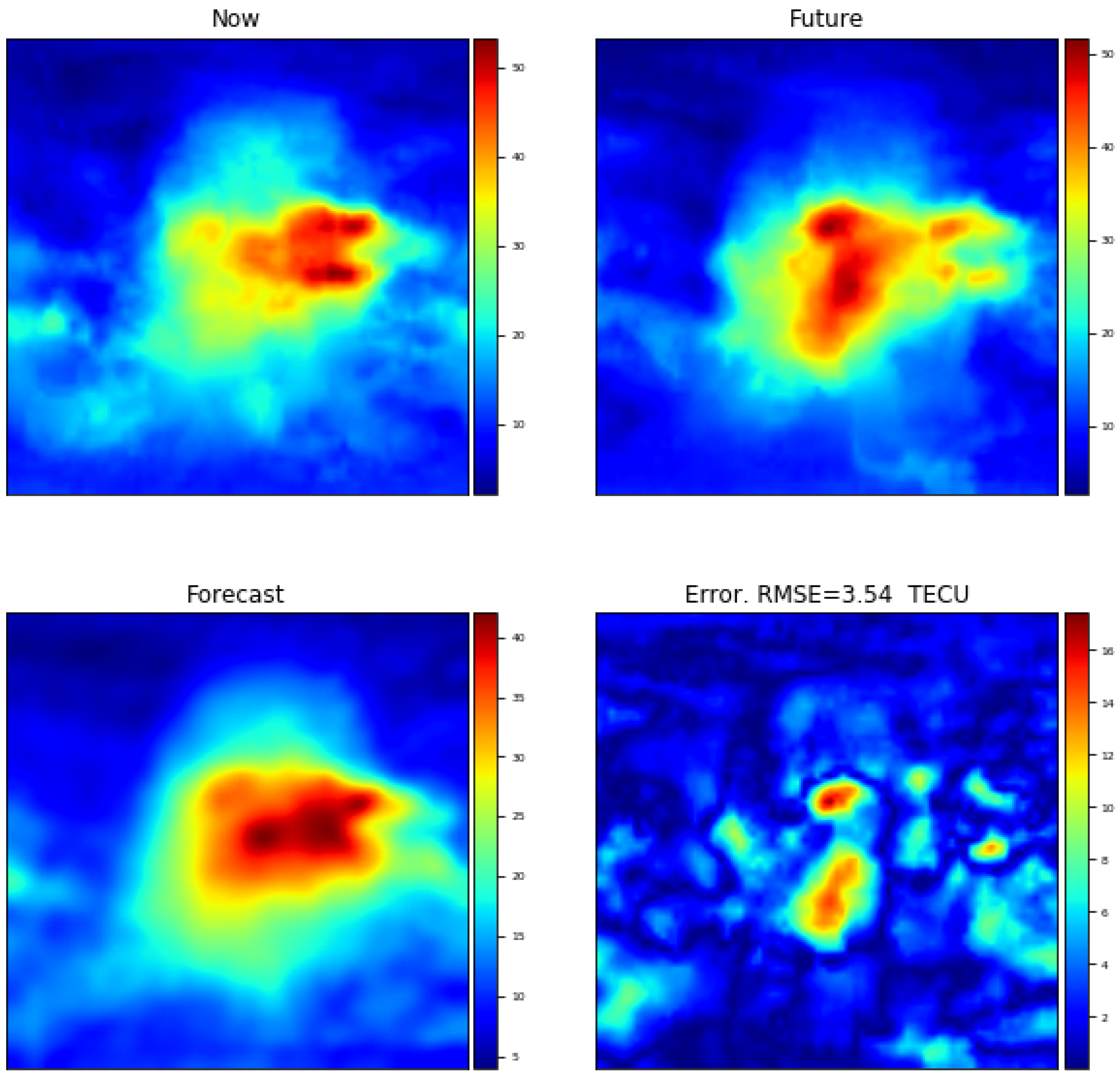
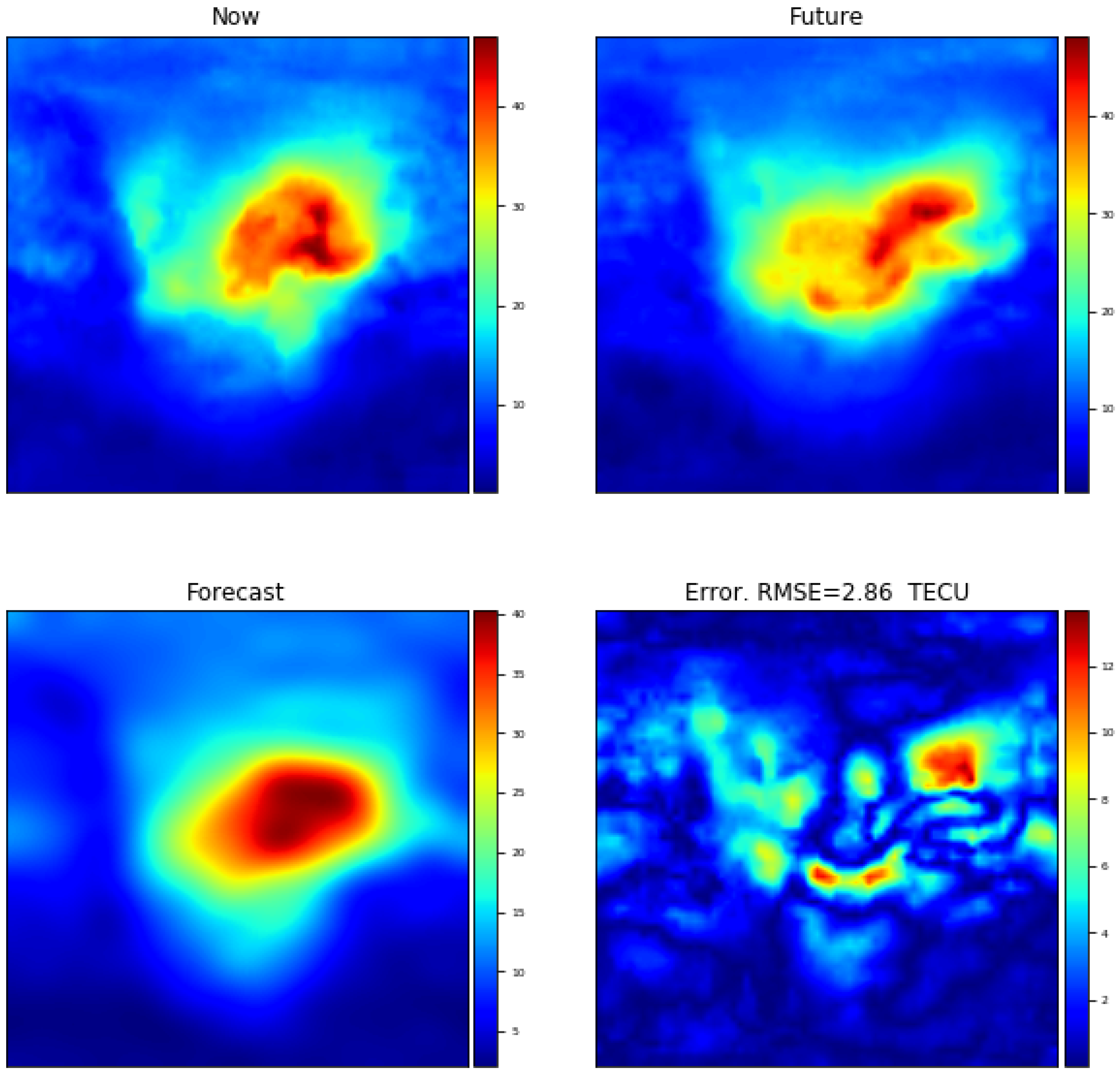
As an example, we present the forecasts at two different times of the year with different solar activity. We decided to select different dates to show that the error at the edges of the high ionization zones occurs in different levels of solar activity. In addition, to show that the effect occurs to a lesser extent in the model we propose in this article. Figure 1 and Figure 2 correspond to the prediction with the DCT method and Figure 8 to the tangent plane method presented in this article. Figure 1 corresponds to the month of May (lower solar activity, see Figure 13), and Figure 2 to the month of February. Figure 8 was computed on the same dates.
The improvement due to the use of tangent planes is evident in the fact that the areas with an error of more than 20 TECUs (Total Electron Content, which is defined as 1 TECU = el/m) are located in much smaller areas of the error maps.
To solve the problem of modeling simultaneously the smooth regions of the maps and the changes on the borders of the high-ionization regions, we decided to use a different basis (in the sense of elements of a linear combination that span a subspace) that allowed for modeling the changes on the borders due to different distortions of the shape of the high-ionization regions. A set of transformations that might allow for modeling the changes at the borders, might be small rotations, small horizontal or vertical displacements, thickening or thinning of the borders, and hyperbolic (shear) distortions. The interest of these transformations resides in the fact that from one time stamp to the next, the changes on the map will be at the border of the ionized region and might be categorized as a mix of the above mentioned transformations.
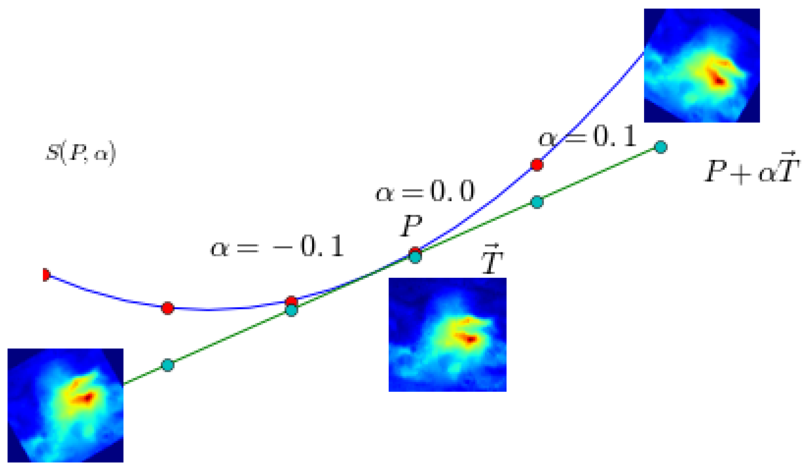
A technique creating the basis that models the changes at the borders of the ionized regions is based on the idea of deformable prototypes. This technique is used in pattern recognition for dealing with common distortions in Optical Character Recognition (OCR) (see for instance, [29,30,31]). The idea assumes that the image, in our case a map denoted as P, is a point in a high dimensional space. Each pixel map P is considered as a point in a space of dimension , i.e., . For modeling the local changes from one map to the next, we assume a transformation that creates another image, parameterized by . In the exposition of the method, we follow the notation presented in [30].
In Figure 3, we show a diagram of the method. Note that given a point P, we can create a trajectory in the space , by introducing small linear changes along directions in this space. In the example of the figure, the distortion, parameterized by , consists on a rotation of the map. Thus, we denote the set of points x in for each rotation as the set for which . In the figure, the trajectory followed by x, i.e., new images obtained from small rotations of P, is represented by a parabola, which is a one-dimensional curve embedded in the space of possible maps . Note that, knowing the value of the pixels of the map P, and the structure of the transformation (in this case a rotation), we can characterize the trajectory in as a manifold, and one can compute the tangent vector at that point. The tangent vector is represented by a line that intersects the curved manifold at P, and is represented by the vector . For small values of , we can approximate by the Taylor expansion around :
As an example, if we allow for another transformation, such as a vertical translation, we would have a different trajectory along a one dimensional manifold with the corresponding tangent vector. Hence, two tangent vectors, and , will define a tangent plane, and we can construct a first order approximation to a change on the map/point P by both transformations as a new point on the tangent plane:
Generalizing with the above example, we denote the estimate of the forecasted map at a future time value as , which is a function of the current map at time plus a point in the tangent plane spanned by the set of tangent vectors . The tangent space is defined by the list of distortions/transformations that we define in the following list:
{X/Y-translation, Thickening/Thinning, Rotation, Parallel Hyperbolic, Diagonal Hyperbolic}
The parameter h allows for modeling the fact that the forecasting horizon might be different from the sampling rate. The forecast at horizon can be expressed as follows,
A criterion for determining the value of the weights of Equation (3) might be the minimization of the norm of the error between the observation at , and the combination of the observation at , along with a linear combination of the components of the tangent space , that is:
Note that, as the dimension of P is much higher than the number of parameters , the problem is well posed. The initial model of Equation (4) can be extended and improved, taking into account the fact that the ionization regions change slowly in time, and therefore we could use a set of previous maps to give a better forecast. The tangent spaces of the previous maps are also computed, and are combined linearly with the set of previous maps. This gives rise to two possible strategies for the estimation of the forecast:
- (a)
- For each past map , estimate the values of for each element of the tangent space by means of Equation (3), giving the partial estimate at from map i, . Afterwards, the final estimation is done by a linear regression of each partial estimate.
- (b)
- Compute the tangent spaces of each of the maps , and do a linear regression using the N maps and the tangent space.
Although a linear combination followed by another a linear combination is equivalent to a single linear combination, from the estimation point of view, the coefficients obtained by method (a) are different from the ones obtained by (b). In the preliminary experiments (done using data of the year 2014), we have found that although the estimation method (a) allowed us to interpret the forecaster, and use tests of significance in order to asses the number of past maps relevant for the forecast. Nevertheless method (b) gave a better performance in the RMSE sense. An additional insight that we obtained from (a) was that the relevance of the previous snapshots for forecasting the future was not uniform along time, i.e., sometimes the most relevant snapshots were in the past few minutes, and in other cases the relevant snapshots were up to a few hours in the past.
For methodological reasons, we used the data from year 2014 as training for determining the structure and algorithms, and data from year 2015 as an independent validation and contrast dataset, and finally data from year 2016 to characterize the performance of the new forecasting model, i.e., the results are derived from data not seen when computing the parameters of the model and when deciding its structure. This methodology was done to diminish the possible effect of overfitting and selection bias. In the preliminary experiments, we tested different machine learning techniques [32]. For selecting the forecasting algorithm, we evaluated two experimental frameworks,
- (a)
- Use a historical set of values (one year) to estimate the parameters of the forecasting technique. This method has the advantage that can be used with a large set of machine learning algorithms. As a drawback, leads to complicated models that have to take into account all possible features of the time evolution of maps. Most machine learning algorithms can be trained with this approach. In particular, we evaluated linear regression, LASSO, clustering (k-means), CART and neural networks (MLP).
- (b)
- Use only data from a limited number of maps prior to the current one. A drawback of this method is that it can only be used with regularized linear regression . This is because the other methods need a much higher number of examples. The advantage of this approach is that one can deal with the fact that, although the ionization pattern is similar over large regions, there is high variability of both the shape and morphology of the ionization regions in the time series of maps. The shape of the borders of the ionization regions changed slowly and the rate of change at different parts of the borders was not uniform. This justified both the introduction of the tangent space, which models the local changes, and the estimation of the coefficients of a linear regression with local data to select the relevant components.
The preliminary experiments showed that the method produced a greater error than . We discarded other methods such as neural networks, SVM, and CART because of the infeasibility of training the models with approach .
As the evolution of the region of highest ionization was slow in the TEC forecasting case, and the changes between different time epochs were concentrated at the borders of the regions of highest ionization, we decided to use a method that took into account the small distortions. This was done by computing the tangent vectors (also called the Lie derivatives) for different kinds of locally spatial distortions. As each tangent vector in the space of dimension 5112 can be represented as an image of , the forecast consisted of a linear combination of past maps and their respective set of tangent vectors for a set of distortions (for geometrical and algebraic details see next subsections).
3. Description of the Tangent Space Method
In this section, following [30], we define the equations for computing each of the the tangent spaces of the list of distortions defined in Section 2. A difference between the implementation for forecasting TEC maps and the one proposed in [30] for OCR is that we did not smooth the finite difference approximation of the derivative. In the case of OCR, this smoothing is done by means of a 2D low pass filter and it is necessary in order to assure a smooth curvature of borders of the new template. In our case, we tested different smoothing techniques, such as linear low pass filters, and total variation smoothing, which resulted in a deterioration in the performance. Therefore, we approximated the derivative by a finite difference without smoothing:
The finite difference is computed using second order central difference in the interior grid points of the map. At the boundaries of the map, the derivative was approximated by a first order difference between each border point (i.e., TEC value) and the corresponding nearest inner grid point.
That is, for the interior grid points of the map, the discrete approximation was computed as follows:
and
For the border points of the map, the discrete approximation was computed as:
and
We construct the tangent vector for each of the possible seven transformations:
{X-translation, Y-translation, Rotation, Parallel Hyperbolic transform, Diagonal Hyperbolic transform, Thickening and Thinning transform}
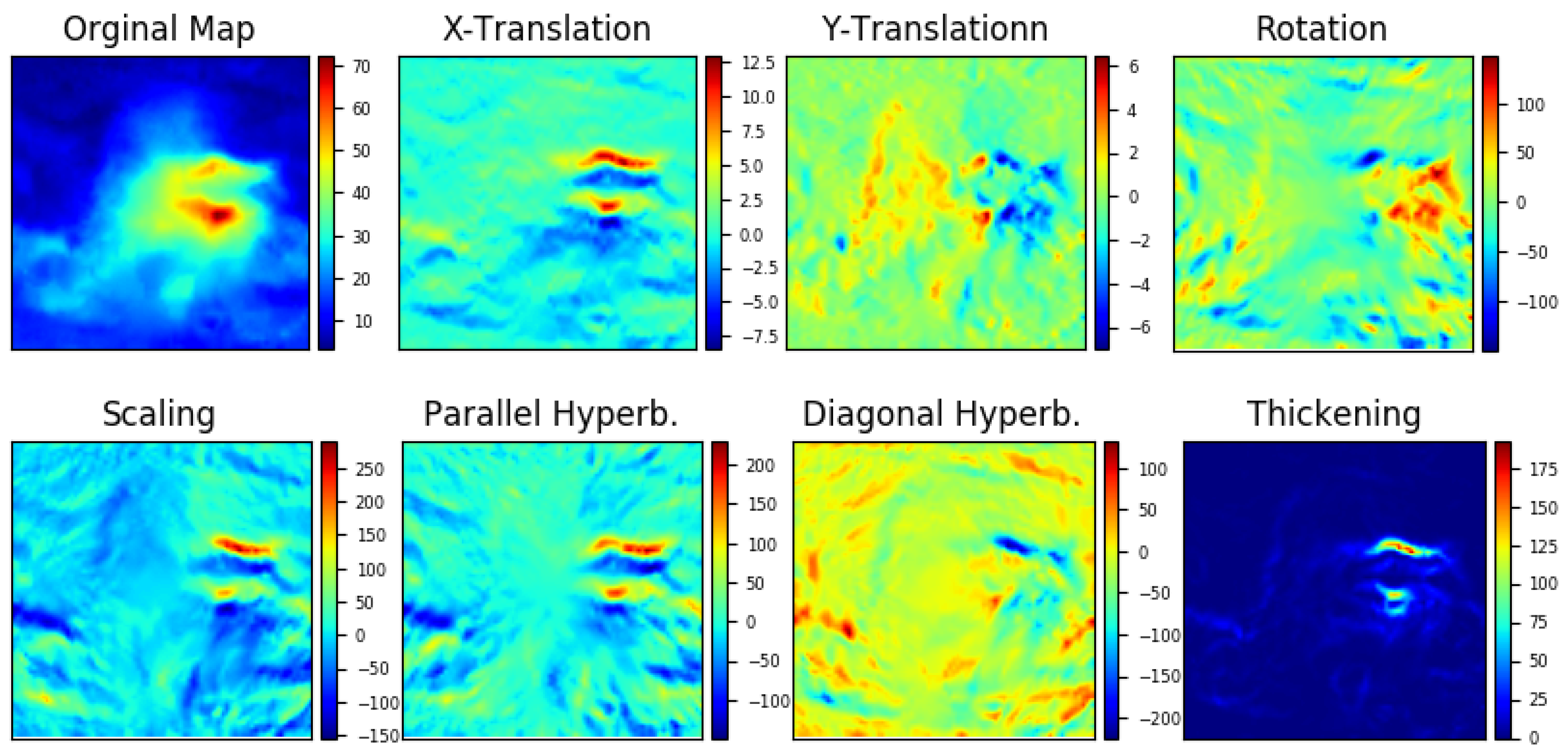
We define all operations with reference the origin of coordinates at the center of the map, which in our case is: , and the local perturbation for each distortion is denoted by . In Figure 4, we show the tangent spaces for a given map (upper left) observed at time stamp “2016-02-21 13:30:00” (Year-Month-Day Hour:Minute:Second). The equations that define each of the directions that span the tangent space are the following:
- X/Y-translation:The corresponding Lie operators are defined as: and .
- Rotation by a small angle :The corresponding Lie operator is defined as: .
- Parallel/Diagonal Hyperbolic transformation:The parallel hyperbolic transformation defines a shear transform (left), and the diagonal hyperbolic transformation (right) defines a squeeze mapping.The corresponding Lie operators are defined as:(parallel) and (diagonal).
- Thickening and Thinning transformation:The corresponding Lie operator is defined as: .
- Scaling transformation:The corresponding Lie operator is defined as: .
Transformation of a Map along the Tangent Directions
The effect on a map of a small perturbation in the direction of each of the components of the tangent space is summarized in Figure 5, Figure 6 and Figure 7. Each figure presents two groups of maps, corresponding to two different directions in the tangent space. In Figure 5, we show the effect of moving the map, along the “rotation” direction (left group), and along the “Thickening” direction (right group). The left group of four maps show the original map (upper left), the tangent map for a small rotation of the map, and (lower) two reconstructed maps for opposite directions. The effect is moving the map either along the positive direction of the tangent space, i.e., rotates slightly the map clockwise, or along the negative direction anticlockwise. Note that a shift of value in this case not only implies a noticeable rotation, but also increases the background level of ionization. Analogously, the tangent direction related with a thickening/thinning transformation (right), increases the area of the ionized region when added (thickening) , and reduces the area (thinning), when subtracted, i.e., . In Figure 6, we show the effect of a Scaling transform (left group), and a shift in the vertical direction (right group). The effect of the scaling transform is a diagonal displacement of the ionized region, while the effect of the vertical shift is barely noticeable. This highlights that the size of the factor can have different scales. In practice, as it can be seen for instance in Figure 9, the value of the weight of each dimension of the tangent space has different size, that is the value of can take values in a wide range. While the terms related to rotation are small, the term related to the Y-translation is much higher. A value gives rise to a clear rotation of the ionized area in Figure 5, but the same value barely changes the map, as shown in Figure 6 (right). The case of a horizontal shift is analogous to the case of the vertical shift.
In Figure 7, we show the effect of the hyperbolic (shear) transforms of the map, which accounts for diagonal deformations of the map. Note that, in this case, the scale of the factor increases the background ionization level, while it models reasonably well the changes in the highly ionized region. This effect of changing the background ionized level will be taken into account in the forecasting model by introducing a bias term in the forecast, .
4. Model of the Forecaster
4.1. Structure
In this section, we present the model for the forecasting of the maps at a given horizon. This model is based on the ideas presented in Section 2.
In univariate time series (see, for instance, [33]), the forecast model sometimes consists in a linear combination of the past samples. In our case, the analogy will consist in a linear combination of the time series of the last N maps ,⋯, , with the corresponding tangent spaces. In the selection of the past lags, we took into account the fact that the general patterns of ionization have a main periodicity of about one day. Thus, along with the maps inside a time window near the current observation, we selected a time window at approximately a time lag of about 24 h prior to the current map. The problem of model selection and model estimation is well known in machine learning (see, for instance, [32], Chapters 7 and 8). The case of time series is an especially difficult problem due to the correlation between samples and the presence of cyclical patterns of different origins and scales.
For methodological reasons, we divided the data into three sets to decouple the process of selecting the structure and the parameters of the model. For each potential configuration of the forecasting model (i.e., set of lags for previous maps and tangent spaces), we defined the optimal set of delays and estimation algorithm during the training year, i.e., 2014, and validated the performance for the different configurations with the RMSE evaluated on data in year 2015. Finally, independent data from year 2016 was left for reporting the performance. The list of time horizons we use in this work is the following: = {1/2 h, 1 h, 2 h, 3 h, 6 h, 24 h}.
The structures for the forecasting that were evaluated included different time lags prior to , and time lags centered at multiples of 24 h before . In addition, there was the possible inclusion of the tangent maps, with their possible combinations.
An interesting result is that the best performance was obtained when using as delay lags multiples of the forecast horizon, and the inclusion of a neighborhood of .
The general structure of the models for forecast at horizon h included the use of the list of delay lags summarized in Table 1.
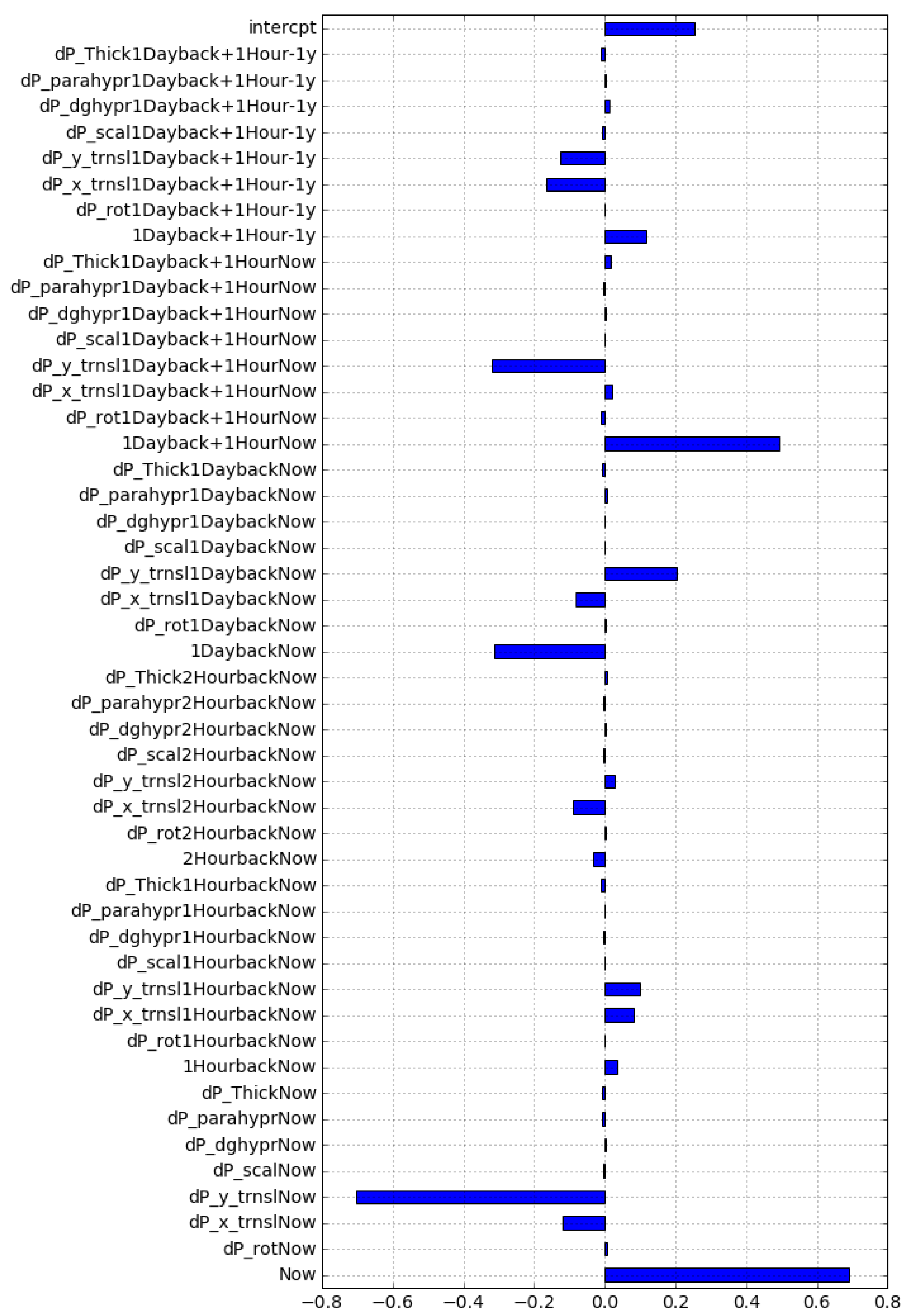
In Figure 9, we plot the values of the estimated parameters , for a forecasting horizon of h = 1 h. This plot shows that the terms corresponding to the delay in the neighbourhood of (i.e., one day) had a significant contribution. This effect was much lower when the delay lag was 48 h, which we decided not to include because the use of this delay did not improve the performance on the validation database (i.e., year 2015), and increased significantly the complexity of the model. Another effect that consistently appeared in most of the experiments was that most of the contribution to the forecast came from the current map, along with its tangent space, and the forecasting power of greater lags diminished quickly. Thus, the context for forecast is limited to . In addition, to model the fact that there might be a global change of the ionization, we introduced an intercept . The forecasting was done by means of the following formula,
The set of elements of the tangent space are summarized in , and explained in detail at the Section 3.
4.2. Parameter Estimation
In this subsection, we argue the criteria to select of the estimation algorithm for the model presented in Equation (14). The model consists of a linear combination of maps, weighted by the coefficients and , which can be estimated with different criteria. That is, we set a structure of delays, and the values of the coefficients are determined at each forecasting step by minimizing a cost function, and therefore making the forecast robust with respect to the solar maximum/minimum conditions. In analogy to Equation (4), we minimize the forecast error with some restrictions on the possible weights. Note that the estimation of the parameters is done using only the near past of the map at time . Specifically, to estimate the parameters of the model, we used as time indices the row “Training” at Table 1, and the forecast was done using the time indices at the “Forecasting” row. Note that, in the same table, in the lower row, we define the notation of the weights associated with each delay.
The use of only the last few samples (i.e., just the samples in the row “Training” of Table 1) for the estimation of the weights is justified by the empirical fact that the performance of the forecaster, exhibited a better RMSE. When the estimation of the parameters (i.e., the training) is done using the whole year, the resulting performance was significantly worse. The explanation is that the local (in the temporal sense) variation of the maps has a greater contribution to the relative weighting of the past samples and tangent space than a fixed set of weight computed from a long time series.
A drawback of using a small set of samples for the estimation of the parameters is that the system of equations might be underdetermined and will suffer of problems of collinearity. Therefore, to deal with this problem, the criterion for the estimation of the parameters has a regularization term. This regularization term consists on a penalization of the norm of the weights. In the case of using norm , the method is known as Ridge Regression , and, in the case of using norm , the method is known as LASSO (see, for instance, [32] Chapter 3). The difference between both norms is that the Ridge Regression introduces a constant in the diagonal of the covariance matrix which results in a uniform decrease in the value of the estimated parameters, while in the LASSO algorithm the parameter determines the level of sparsity, i.e., the number of parameters with a value equal to zero.
The optimization criterion is presented in Equation (15), where the regularization term corresponds to Ridge Regression when , and LASSO when . We also considered the use of norm in the error term, i.e., . This norm penalizes small values of the error, and the influence of the outliers on the estimated weights is small. In our problem at hand, the use of this norm on the error term gave a much higher proportion of maps with at least one negative value of TEC. Therefore, we selected as norm for the error term, giving the following cost function. In the implementation done in this work, the results are presented using the Ridge Regression regularization, and the was selected by cross-validation on the data from the year 2014. The difference in performance obtained from using Ridge Regression or LASSO was negligible, and the Ridge Regression was selected because the running time was faster.
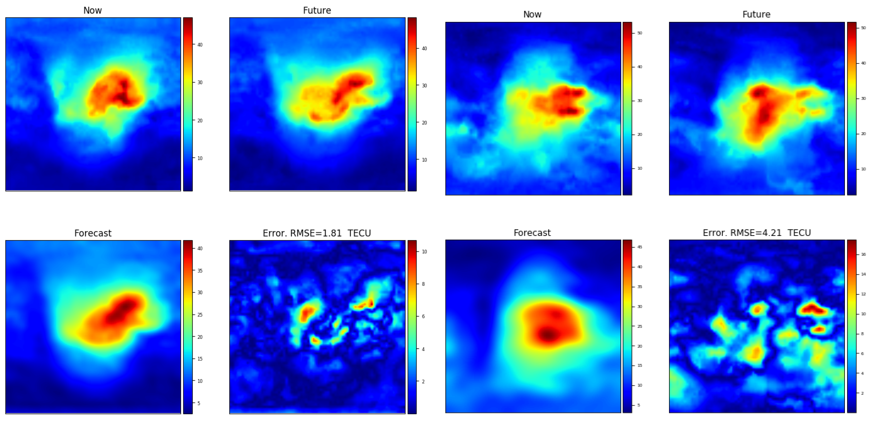
A typical example is shown in Figure 8, where we present the forecast at a horizon of 3 h, at two different time stamps, i.e., at 2016-05-12 15:15:00 (left) and 2016-02-21 13:15:00 (right). For comparison purposes in Figure 1 and Figure 2 we show an example of the performance when using a DCT forecast in the same conditions. The benchmark that we will follow for determining the performance of the system will be the use frozen maps, which we define as the prediction made with the current map keeping its VTEC values constant in a Sun-fixed reference frame, i.e., considering local-time/latitude coordinates. The RMSE ratio between the forecast, and using a frozen map as forecast was of , which as can be seen in Figure 12 is about the mode of the histogram of ratios of the RMSE. The weights associated with the estimate are shown in Figure 9. Note the presence of a positive intercept or bias , which models both, the contribution of the background ionization of the different elements that are combined linearly and that the possible increase of the background ionization. In addition, note that the main contribution to the forecast, come from the current map, with a strong negative component of a vertical deviation. The third most important contribution to the forecast is related to the map at h, with its tangent space along the vertical direction. On the other hand, the contribution of the maps at 1 and 2 h in this case is marginal.
The forecast map (lower right) is much smoother than either the current map or the target map . In addition, the distribution of the error reproduces the observation that the borders of the ionized region accumulate most of the error; in this case, in part of the border, the error reaches a maximum of 9.5 TECUs.
The forecasted TEC values were always positive (in the train and validation years), except for a small fraction of cases in the 30 min and 1 h forecast. In the case of the forecast at 1 h, there were only 123 maps that had at least one negative pixel, of a total of 34,536 (i.e., a whole year). In this case, the negative values can be substituted by the values of the Frozen prediction at the latitude/longitude where the forecast was negative.
5. Results
In this section, we summarize the performance of the forecast system based on the tangent spaces. The first results consist in the comparison of the error in the sense of total TEC RMSE (i.e., the mean value for all the pixels of the map). We compare the forecast by using tangent spaces (which we denote as tangent space method) with a forecast created considering no changes in the map in a mostly Sun-fixed reference frame (local-time vs. latitude),which we denote as frozen map method.
Given a time series of maps, for the map at time consisting of the TECU value and the estimated values , the RMSE was computed as:
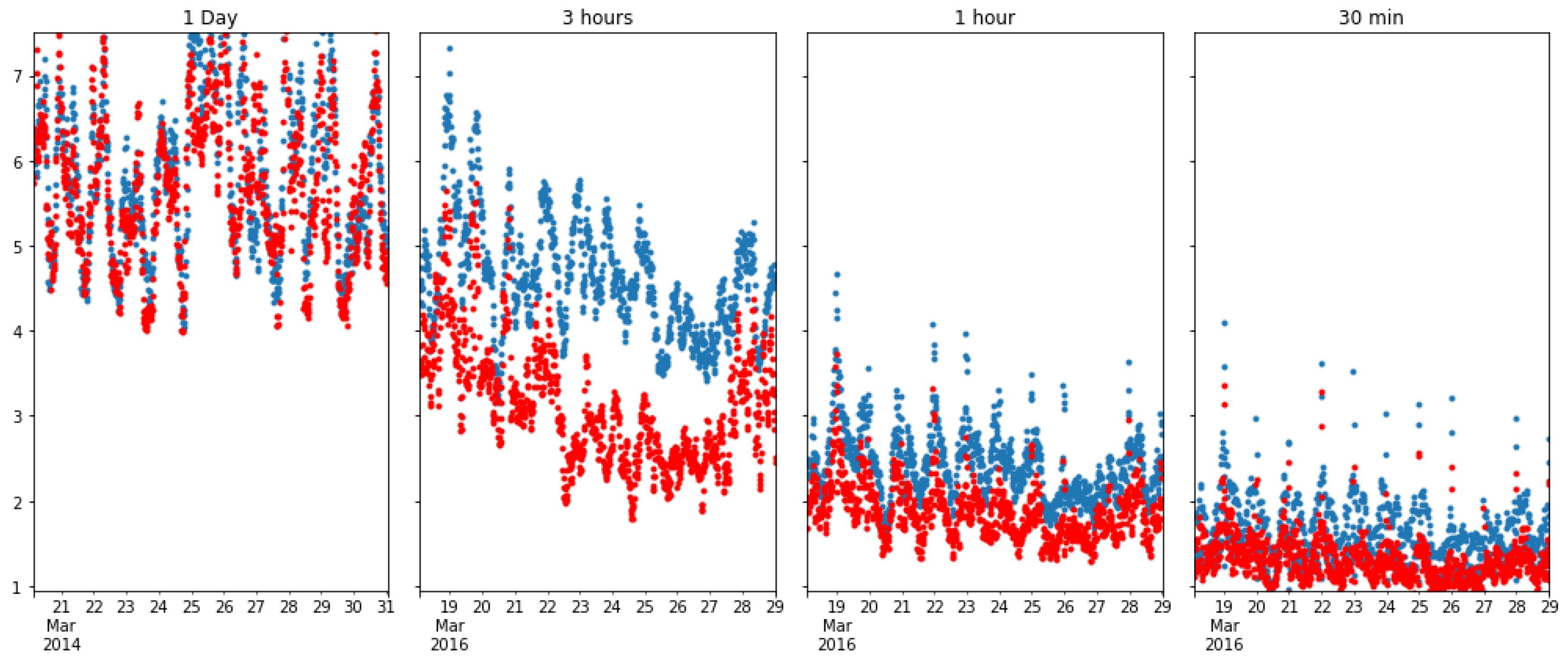
In Figure 10, we show a comparison of the forecast RMSE time series for the tangent space method with the frozen map method during an interval of 10 days during the month of March 2016. In the figure, the comparison between methods has been done for horizons of 30 min, 1 h, 3 h and 1 day. The RMSE time series for the tangent space method (red), is systematically below the frozen method (blue) for the cases of 30 min, 1 h and 3 h, with periodicity of the error of about a day. In the case of the horizon at 1 day, the forecasting error is the same for both methods. The RMSE results are computed as a mean over all the map, and as mentioned in Section 2, the main contribution to the error originates from the borders of highly ionized regions. Therefore, the TEC values presented in this subsection are an average between low error regions and these borders. The result is representative of the general behavior of the algorithm, and is compatible with the results averaged over an entire year, as shown in Table 2.
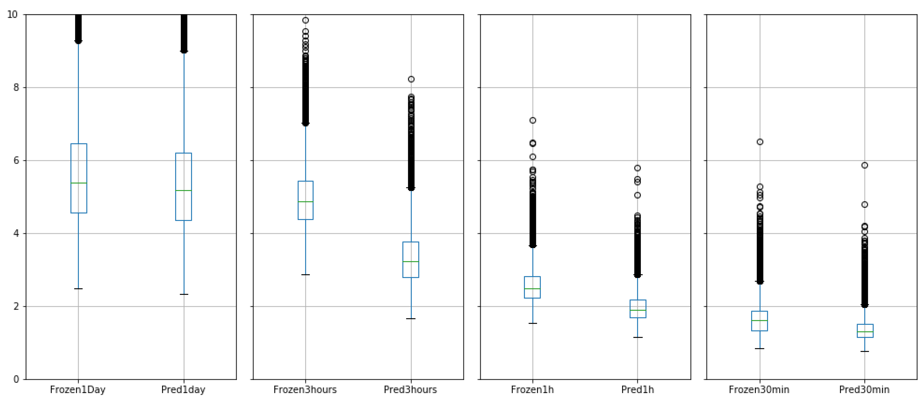
In Figure 11, we present the boxplots (see [34]) of the forecast errors for different horizons, computed for a whole year. One can see that, in all cases, except for one day, the forecasting error in terms of forecast RMSE obtained by tangent space method was better than using a frozen map. The proportion between of improvement is summarized in Table 2. The improvement not only refers to the median value, but also to the range of the errors between the external whiskers (defined as the range between the quartile (i.e., the percentile ) less times the interquartile range, i.e., the difference between (i.e., the percentile ) and , that is, the first datum greater than and the other extreme is given by the last datum less than ). As can be seen in the figures, the dispersion around the mean corresponding to the tangent space method is lower, in the senses that it encloses a smaller margin, and also in the sense that it systematically has a lower value. Another feature is the lower prevalence of high values of the outliers in the case of the tangent space method.
In Table 2, we show the ratio of the root mean square error (RMSE), of the tangent space method vs. the frozen map method. The RMSE in this case is computed as a mean over the , maps corresponding to a year, where each forecast is made every 15 min. The RMSE was computed as follows:
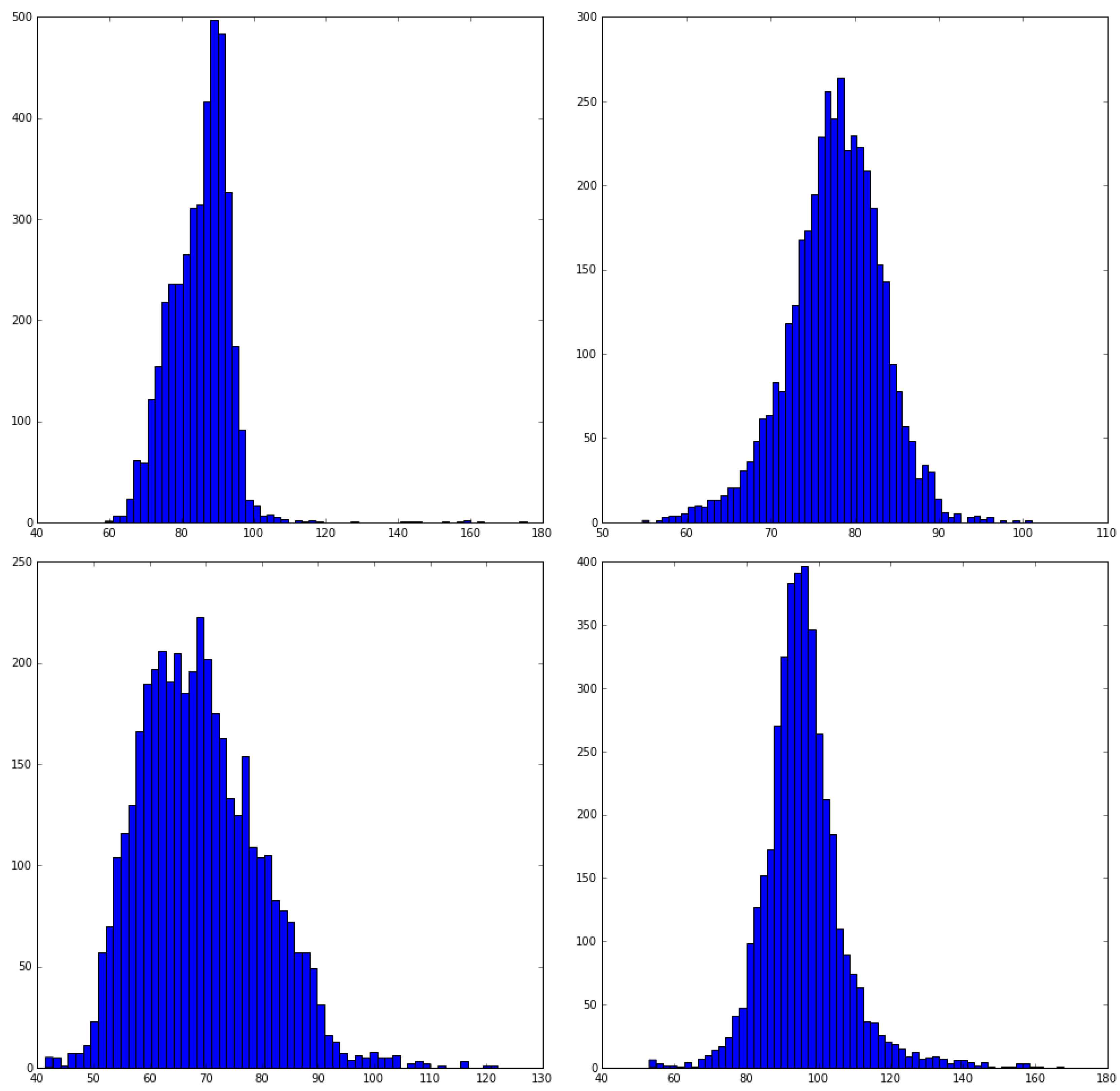
In the table, it can be seen that, in all cases, the ratio of forecast RMSE is below , that is the tangent space method gives a lower RMSE forecast in mean. In Figure 12, we show the histograms of the ratio for a time interval of 42 days. Note that the maxima of the histograms coincide approximately with the mean values shown in Table 2, which is due to the low variance and skewness of the histograms. Note also that, as the coefficients of the tangent space forecaster are computed for each forecast, the results performance of the method is not biased by the solar cycle, that is, we have seen empirically that the total RMSE is proportional to the underlying mean TEC. Thus, although the tangent space method is better than freezing, the RMSE will also depend on the solar cycle conditions.
The results for different horizons show a performance that follows a convex shape, with a minimum error at a 3 h horizon. In particular, the performance at h and at 6 h has a mean value of about , which worse than at horizons of h. In the case of h, this is due to the fact that the rate of change of the state of the ionosphere is slow, and at this horizon there is small room for improvement in the forecast. This small change of the state of the ionosphere is reflected in the fact that the RMSE due to freezing is in mean about 2 TEC, which is lower than at other forecasting horizons, as shown in Figure 10. Interestingly, in the histogram shown in Figure 12, the number of samples with error greater than is much higher than in the other cases and also the upper values are much higher, which is attributed to the fact that the histogram is a ratio between numbers that can be small.
A trend that can be seen in Figure 12 and in the boxplots is that the spread of the forecast errors errors increases as a function of the horizon. Nevertheless, note that, as reflected in Figure 12, the tangent space forecast for intermediate horizons gives a lower limit of the % of error, and the number of samples for an error greater than is much lower. Which indicates that the quality of the tangent space forecaster in the sense of total RMSE is better than in the case of freezing, in all the horizons except 24 h.
On the other hand, at a horizon of 6 h, the performance degrades, being comparable to the performance at h, which indicates that the hypothesis of small changes in the tangent space (see Section 3), begins to not be entirely valid. Finally, at a horizon of 24 h, the performance does not differ much from freezing the maps, which indicates both, that the hypothesis underlying the model of tangent spaces does not hold, and that also that a simple linear combination of past observations is not enough for modeling a TEC map at one-day horizon. The forecast by means of the tangent space is slightly better than just freezing the last observation, Figure 12 shows that the ratio between the performances of the two systems has a shape similar to a Gaussian, with a mean at , with a standard deviation nearly . On the other hand, the boxplots in Figure 11 (left) show a median RMSE of 5 TECUs, which might not be acceptable. Note that, although we have found that the component at 24 h is relevant for the forecast at short term horizons, it does not seem adequate for a forecasting at such a long horizon. That is, for short-term predictions, the maps at 24 h in advance complements the information from the last observation and helps to improve the forecast by making use of the periodicity of the ionization patters. On the other hand, when the horizon is directly 24 h, the information yielded by the last observation is not enough for a good forecast.
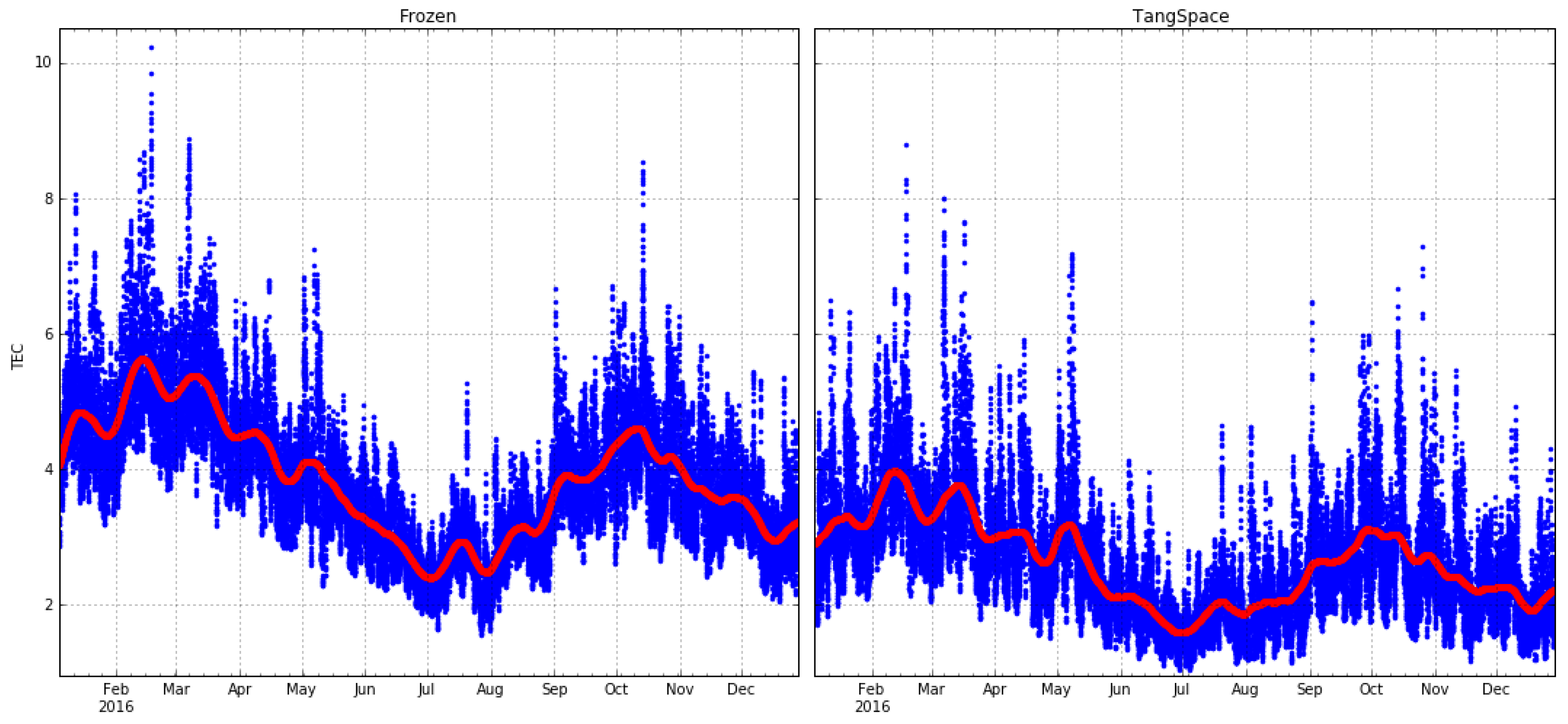
For comparison purposes, in Figure 13, we show the time evolution of the RMSE in TECUs for a whole year and a different forecast horizon (3 h). The figure consists on the superposition of the instantaneous RMSE and the low pass filtered (zero phase, moving average with a cut off frequency of 1/(0.5 month) time series. The shape of the temporal evolution of the RMSE over a whole year is similar for the other forecast horizons. The first feature that we notice is a seasonal component with a maximum activity at spring and autumn and a superposed a cyclic component with a period of 28 days. In the case of the forecast by means of the tangent space model, the difference between the maximum and minimum of the low pass filtered version is of TECUs, with a mean value in spring of about TECUs, in summer of 2 and in winter of TECUs. The variability of the error is much lower in summer. The variability is much higher than would be expected in the case of a Gaussian distribution (see Section 5.4), with local peaks over 6 TECUs occurring only certain moments in 14 days of the time series. A test was done with the years 2014–2015, where the activity was higher, and the results were analogous, with a systematic increase of the low pass filtered RMSE of 1 TECUs. Note that, from a methodological point of view (of machine learning), this analogy is merely indicative, because these years were used for determining the structure of the forecaster.
5.1. Improvement on the Forecast Due to the Use of the Tangent Space and Comparison with the DCT Forecasting Method
In this section, we compare the proposed approach with a forecasting system that does not use tangent spaces but just the original VTEC maps (labeled Maps Only) and with one based on the DCT (DCT method). In both cases, the number of free parameters of these models is lower than that in the tangent model, which means that the comparison is not in equal terms. On the other hand, a possibility of doing this comparison with an equal number of degrees of freedom would be to use a number of maps equal to the number of elements in the tangent map. In this case, either if we took maps further in the past, which are increasingly different from the map to be forecasted, or if we increased the number of recent maps, highly correlated inputs are given and therefore we have a badly conditioned problem. The improvement due to the use of the tangent spaces is shown in Table 3. The result is that the use of the tangent space coefficients improves the forecast result in all horizons, except for 24 h. In all cases (except for the horizon of 24 h), the use of tangent space improves the results to the DCT method. The 24 h case is explained by the fact that the tangent spaces model local distortions, which do not account for the changes at such a long range. Note that the confidence margins (standard deviations) are not shown, because using 34,626 maps for computing the mean values of the RMSE gave extremely small values.
5.2. Performance as a Function of the Latitude
Next, we analyzed the performance of the algorithm as a function of the latitude. We analyzed the whole year 2016 and we set a horizon of 1 h, with a total of 34,626 maps. Note that the test year is different from the years used for determining and validating the structure of the forecaster. For presenting the results, we have selected a horizon of 1 h to show the performance in a situation between the best and the worst case.
The RMSE as a function of the latitude is defined as;
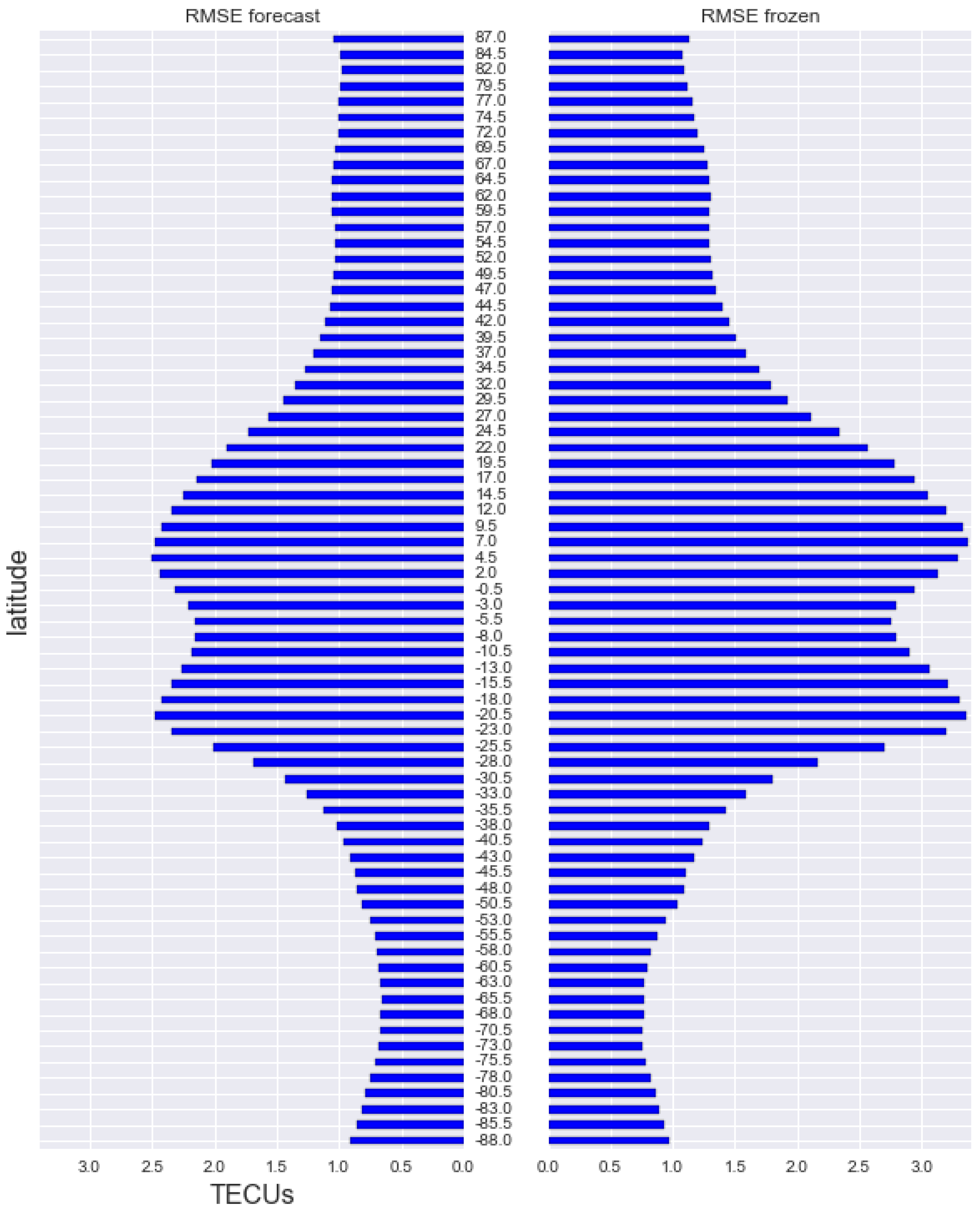
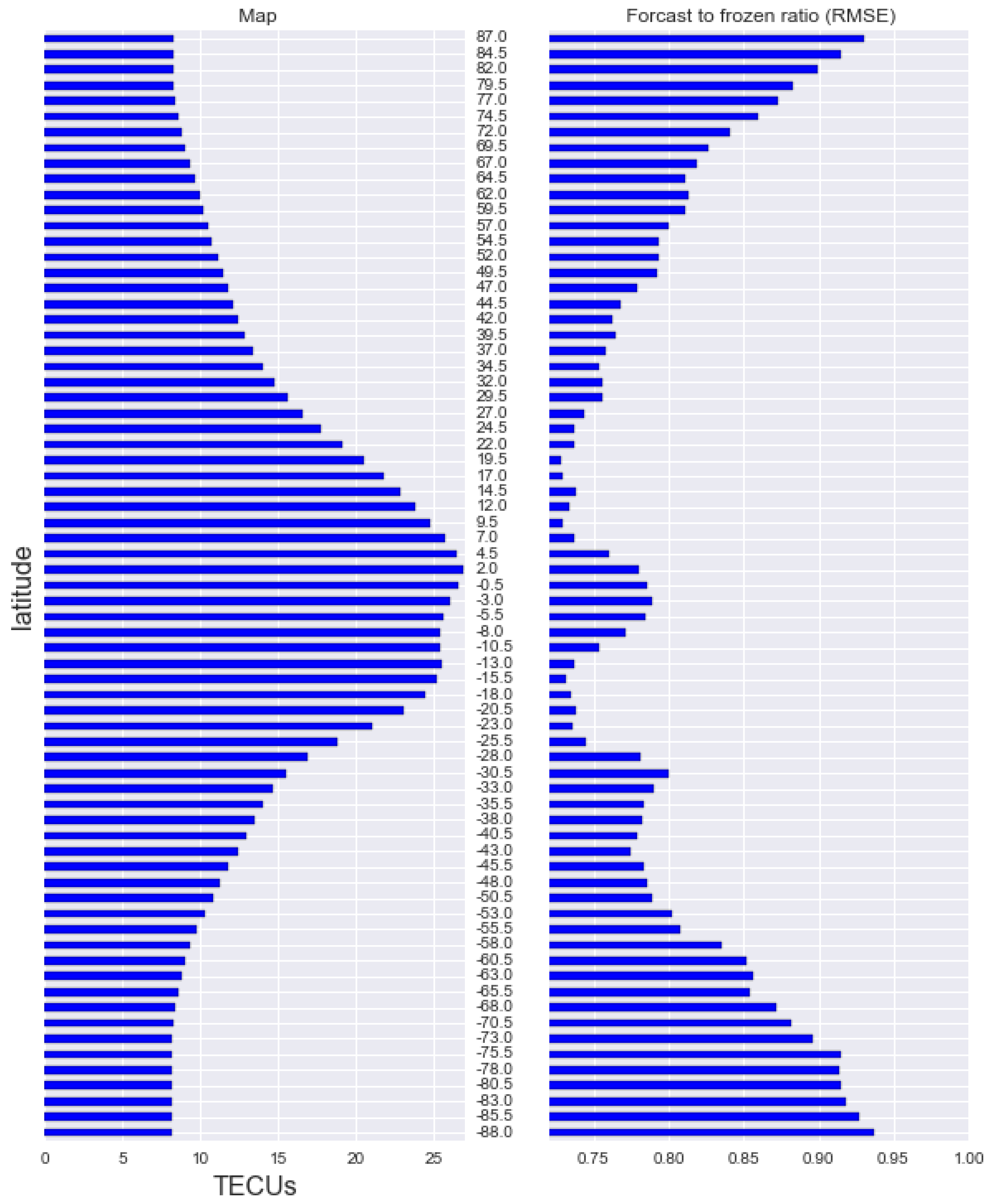
where at the beginning of Section 5. In Figure 14, we can compare, for each latitude the mean value of the RMSE in TECUs of the tangent space method vs. the frozen map method. The results of the tangent space method (left) systematically give a lower value of RMS compared with the frozen map method (right) for all the latitudes, with the most significant improvement between 30 degrees north and 30 degrees south. This is a maximum difference of about 1 TECU for both maxima, i.e., 8 degrees north, and 20 degrees south. On the other hand for latitudes over 50 degrees (north or south), the performance of both methods is similar, due to the fact that ionization activity at these latitudes is much lower than near the equator, and in both cases the RMSE is about 1 TECU. At the equator, there is a dip in the RMSE profile. Here, the tangent distance forecast is better by TECUs. The fact that most of the forecast error is located around degrees and the shape of the profile can be explained from the spacial distribution of the forecast error that tends to be located at the margins of the ionized zone is shown in Figure 8. The distribution of the error on the map also explains the dip on the forecasting error at the equator. In Figure 15, we show the profiles of the Root Mean Square of the values in TECUs, for the whole year 2016 (left) and the ratio of RMSE the tangent space method to the frozen map method (right), also for the year 2016. In both cases, we present the results as a function of the latitude. In Figure 15 (left), the mean TECU values are concentrated around the equator, with a mean value of for the case of latitudes near the equator of about 25 TECUs, and decreasing as the latitudes get near the poles. Note that a first comparison with Figure 14 tells us that the forecasting error in mean is about . This last fact, should be nuanced with the fact that the forecast error is not uniform on the map, but distributed on the borders of the ionized part of the map. In Figure 15 (right), the ratio of the tangent distance forecast to the frozen map shows two minima, located at 9–20 degrees north and 13–25 degrees south, which is about , indicating that the use of the tangent distance forecast produces a reduction of a in mean on the forecast error in the regions of higher ionization. That is the best improvement and is given at two crests of the Appleton–Hartree anomaly, side by side of the equator. Therefore, the tangent distance method is capable of modeling regions with high TEC gradients. Note that the coefficients of the forecaster are re-estimated for each prediction, which means that the movements of the anomaly can be tracked on real time. The forecast improvement at the regions near the pole is lower, but this can be explained because these are regions of lower activity and show a smaller rate of change. This figure hints at the possibility of designing a performance index that might assign a different penalization to the errors depending on the level of activity of related to the latitude.
5.3. Bias Variance Decomposition of the Forecast Error
Next, we analyzed the Bias Variance decomposition of the forecast error, which we define as follows:
For given a map P and the forecasted map , the error can be decomposed as:
where each term is defined as:
and
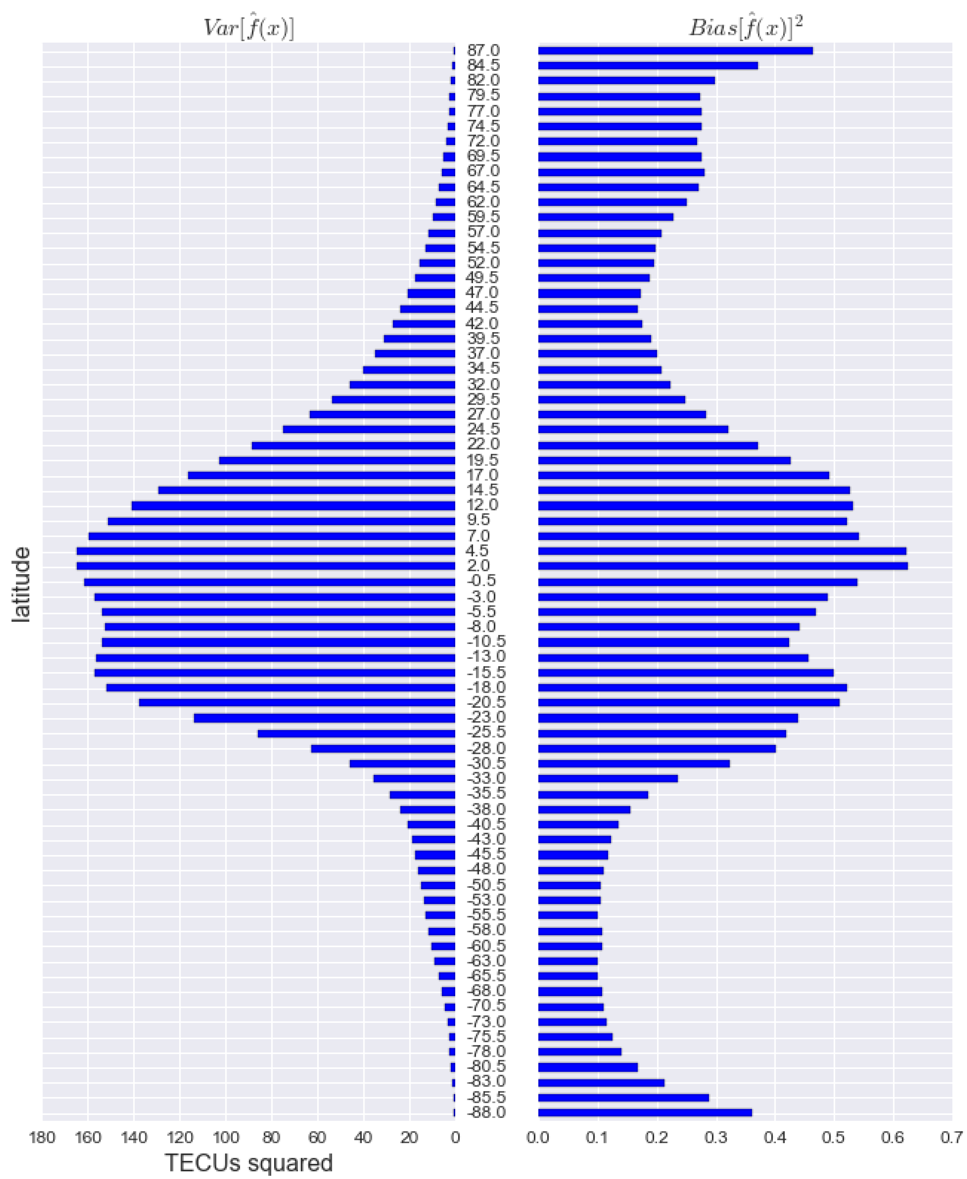
Figure 16 shows the analysis of the contribution to the error of the (left in ) and the (right in ) as a function of the latitude. The variance of the forecast near the equator is of about 12 TECUs, which can be explained by the fact that the main contribution to the error appear concentrated at the borders of the ionized regions, and the variation of this moves in this regions. As it can be seen for instance in Figure 8, the high error values occupy a small part of the map, localized at the edges of the high ionization region. The value of these peaks can reach the order of 9 TECUS, while the error in the inner parts is much lower, of the order of 1 TECU. Therefore, the observed variance should not be understood as the variance of a Gaussian distribution, but as the variance of a bimodal distribution.
On the other hand, the forecast system is almost unbiased (see Figure 16 right): the contribution of the bias to the total error is always less than . Note that the figures have a different scale. The explanation of the low bias of the tangent distance forecast error is associated with the most effective set of parameters describing the degrees of freedom of the system. Note that, in Section 4.2, we comment how we dealt with the fact that the estimation of the parameters might be undetermined.
5.4. Histogram of the Forecast Error
The histogram of the forecast error in TECUs is shown in Figure 17. The histogram is computed for all the pixels of the 34,626 maps, which gives a number of samples greater than 166 million, that is the size of the map times the number of maps, i.e., . In particular, the high error values are located at the borders of the highly ionized regions, and account for the tails of the error histogram. In the log frequency histogram we can see that the distribution follows approximately a line, and can be described by :
, with a p-value less than . This empirical distribution can be approximated by a Laplace distribution (with ):
The linear law fails for values of RMSE greater than 10 TECUs, which is explained by the fact that there are extremely few examples of errors greater than this value. The linear approximation also fails for values of RMSE at lower end, that is <0.75 TEC. The empirical cumulative fraction of errors greater than a given TECU value are presented in Table 4. Interestingly, the accumulated probability diminishes very fast, and Prob( > 4 TECUs) is lower than 1 in 65 pixels, and Prob( > 8 TECUs) is lower than 1 in 8000 pixels. However, as explained in Section 5.3, the extreme values of the errors are isolated in the borders of the highly ionized regions.
6. Conclusions
In this paper, we have presented a forecasting method for TEC maps, based on local information that model possible local distortions. In addition to using several previous maps to make the prediction, we make a decomposition in the space spanned by the components in tangent manifold to each map. The physical justification is that the change at horizons less than 6 h will consist of small changes along the trajectory that is followed by the sequence. The performance has been acceptable for forecast horizons up to 6 h. For a horizon at 24 h, the performance does not differ much from freezing the maps, which indicates both that the hypothesis underlying the model of tangent spaces does not hold up to this time horizon and that a simple linear combination of past observations is not enough for modeling a TEC map at one-day horizon. This is explained because, at this horizon, the changes in ionization have external origins that cannot be derived from the time series.
Author Contributions
Methodology, E.M.M., A.G.R., M.H.-P. and H.Y.; Software, E.M.M. and A.G.R.; Validation, E.M.M., A.G.R., M.H.-P. and H.Y.; Formal Analysis, E.M.M., A.G.R., M.H.-P. and H.Y.; Data Curation, A.G.R.; and Writing—Review and Editing, E.M.M. and A.G.R.
Funding
This research was funded by the project TEC2015-69266-P (MINECO/FEDER, UE).
Acknowledgments
The authors are also grateful to the International GNSS Service (IGS; [21]) for providing GNSS open-data and ionospheric open-products.
Conflicts of Interest
The authors declare no conflict of interest.
References
- Béniguel, Y.; Cherniak, I.; Garcia-Rigo, A.; Hamel, P.; Hernández-Pajares, M.; Kameni, R.; Kashcheyev, A.; Krankowski, A.; Monnerat, M.; Nava, B.; et al. MONITOR Ionospheric Network: Two case studies on scintillation and electron content variability. Ann. Geophys. 2017, 35, 377–391. [Google Scholar] [CrossRef]
- Hernández-Pajares, M.; Juan Zornoza, J.M.; Sanz Subirana, J.; Farnworth, R.; Soley, S. EGNOS Test Bed Ionospheric Corrections under the October and November 2003 Storms. IEEE Trans. Geosci. Remote Sens. 2005, 43, 2283–2293. [Google Scholar] [CrossRef]
- García-Rigo, A.; Roma-Dollase, D.; Hernández-Pajares, M.; Lyu, H.; Li, Z.; Wang, N.; Terkildsen, M.; Olivares, G.; Ghoddousi-Fard, R.; Dettmering, D.; et al. Contributions to real time and near real time Ionosphere Monitoring by IAGs RTIM-WG. In Proceedings of the IAG-IASPEI Joint Scientific Assembly, Albany, CA, USA, 30 July–4 August 2017. [Google Scholar]
- García Rigo, A. Contributions to Ionospheric Determination with Global Positioning System: Solar Flare Detection and Prediction of Global Maps of Total Electron Content. Ph.D. Thesis, Universitat Politècnica de Catalunya, Barcelona, Spain, 2012. [Google Scholar]
- García-Rigo, A.; Monte-Moreno, E.; Hernández-Pajares, M.; Juan, J.M.; Sanz, J.; Aragón Angel, A.; Salazar, D. Global prediction of the vertical total electron content of the ionosphere based on GPS data. Radio Sci. 2011, 46. [Google Scholar] [CrossRef] [Green Version]
- Silvestrin, P.; Berger, M.; Kerr, Y.; Font, J. ESAs second earth explorer opportunity mission: The soil moisture and ocean salinity mission-SMOS. IEEE Geosci. Remote Sens. Newsl. 2011, 118, 11–14. [Google Scholar]
- Krankowski, A.; Hernández-Pajares, M. Status of the IGS ionosphere products and future developments. In Proceedings of the IGS Analysis Center Workshop, Miami Beach, FL, USA, 2–6 June 2008. [Google Scholar]
- Schaer, S.; Société Helvétique des Sciences Naturelles; Commission Géodésique. Mapping and Predicting the Earth’s Ionosphere Using the Global Positioning System; Institut fur Geodesie und Photogrammetrie, Eidg. Technische Hochschule Zürich: Zürich, Switzerland, 1999; Volume 59. [Google Scholar]
- Cander, L.R.; Milosavljevic, M.M.; Stankovic, S.S.; Tomasevic, S. Ionospheric forecasting technique by artificial neural network. Electron. Lett. 1998, 34, 1573–1574. [Google Scholar] [CrossRef]
- Cander, L.R.; Milosavljevic, M.M.; Stankovic, S.S.; Tomasevic, S. Nonlinear prediction of the ionospheric parameter foF2 on hourly, daily, and monthly timescales. J. Geophys. Res. Space Phys. 2000, 105, 12839–12849. [Google Scholar]
- Tulunay, E.; Senalp, E.T.; Radicella, S.M.; Tulunay, Y. Forecasting total electron content maps by neural network technique. Radio Sci. 2006, 41. [Google Scholar] [CrossRef] [Green Version]
- Huang, Z.; Li, Q.B.; Yuan, H. Forecasting of ionospheric vertical TEC 1-h ahead using a genetic algorithm and neural network. Adv. Space Res. 2015, 55, 1775–1783. [Google Scholar] [CrossRef]
- Muhtarov, P.; Kutiev, I. Autocorrelation method for temporal interpolation and short term prediction of ionospheric data. Radio Sci. 1999, 34, 459–464. [Google Scholar] [CrossRef]
- Dick, M.I.; Levy, M.F.; Cander, L.R.; Kutiev, I.; Muhtarov, P. Short-term ionospheric forecasting over Europe. In Proceedings of the IEE National Conference on Antennas and Propagation, York, UK, 31 March–1 April 1999; pp. 105–107. [Google Scholar]
- Stanislawska, I.; Zbyszynski, Z. Forecasting of the ionospheric quiet and disturbed foF2 values at a single location. Radio Sci. 2001, 36, 1065–1071. [Google Scholar] [CrossRef]
- Muhtarov, P.; Kutiev, I.; Cander, L.R.; Zolesi, B.; de Franceschi, G.; Levy, M.; Dick, M. European ionospheric forecast and mapping. Phys. Chem. Earth Part C Sol. Terr. Planet. Sci. 2001, 26, 347–351. [Google Scholar] [CrossRef]
- Krankowski, A.; Sergeenko, N.P.; Baran, L.W.; Shagimuratov, I.I.; Rogova, M.V. The short-term forecasting of the total electron content. Artif. Satell. 2005, 40, 137–146. [Google Scholar]
- Venkateswarlu, G.; Sarma, A.D. A New Technique Based on Grey Model for Forecasting of Ionospheric GPS Signal Delay Using GAGAN Data. Prog. Electromagn. Res. 2017, 59, 33–43. [Google Scholar] [CrossRef]
- Meng, X.; Mannucci, A.J.; Verkhoglyadova, O.P.; Tsurutani, B.T. On forecasting ionospheric total electron content responses to high-speed solar wind streams. J. Space Weather Space Clim. 2016, 6, A19. [Google Scholar] [CrossRef]
- Hernández-Pajares, M.; Juan, J.M.; Sanz, J. New approaches in global ionospheric determination using ground GPS data. J. Atmos. Sol.-Terr. Phys. 1999, 61, 1237–1247. [Google Scholar] [CrossRef]
- Dow, J.M.; Neilan, R.; Rizos, C. The international GNSS service in a changing landscape of global navigation satellite systems. J. Geod. 2009, 83, 191–198. [Google Scholar] [CrossRef]
- Orús, R.; Hernández-Pajares, M.; Juan, J.M.; Sanz, J. Improvement of global ionospheric VTEC maps by using kriging interpolation technique. J. Atmos. Sol.-Terr. Phys. 2005, 67, 1598–1609. [Google Scholar] [CrossRef]
- Orús, R.; Hernández-Pajares, M.; Juan, J.M.; Sanz, J.; García-Fernández, M. Performance of different TEC models to provide GPS ionospheric corrections. J. Atmos. Sol.-Terr. Phys. 2002, 64, 2055–2062. [Google Scholar] [CrossRef]
- Hernández Pajares, M.; Juan, J.M.; Sanz, J.; Colombo, O.L. Application of ionospheric tomography to real time GPS carrier phase ambiguities resolution, at scales of 400–1000 km and with high geomagnetic activity. Geophys. Res. Lett. 2000, 27, 2009–2012. [Google Scholar] [CrossRef]
- Feltens, J.; Angling, M.; Jackson-Booth, N.; Jakowski, N.; Hoque, M.; Hernández Pajares, M.; Aragón Angel, A.; Orús, R.; Zandbergen, R. Comparative testing of four ionospheric models driven with GPS measurements. Radio Sci. 2011, 46. [Google Scholar] [CrossRef] [Green Version]
- Hernández-Pajarez, M.; Roma Dollase, D.; Krankowski, A.; García Rigo, A.; Orús Pérez, R. Comparing performances of seven different global VTEC ionospheric models in the IGS context. In Proceedings of the International GNSS Service Workshop (IGS 2016), Sydney, Australia, 8–12 February 2016; pp. 1–13. [Google Scholar]
- Roma-Dollase, D.; Hernández-Pajares, M.; Krankowski, A.; Kotulak, K.; Ghoddousi-Fard, R.; Yuan, Y.; Li, Z.; Zhang, H.; Shi, C.; Wang, C.; et al. Consistency of seven different GNSS globl ionospheric mpping techniques during one solr cycle. J. Geod. 2017, 92, 691–706. [Google Scholar] [CrossRef]
- Gonzalez, R.C.; Woods, R.E. Digital Image Processing; Addison-Welsley: Boston, MA, USA, 2008. [Google Scholar]
- Simard, P.; LeCun, Y.; Denker, J.S. Efficient pattern recognition using a new transformation distance. Adv. Neural Inf. Process. Syst. 1993, 5, 50–58. [Google Scholar]
- Simard, P.; LeCun, Y.; Denker, J.; Victorri, B. Transformation invariance in pattern recognition tangent distance and tangent propagation. In Neural Networks: Tricks of the Trade; Springer: Berlin, Germany, 1998; pp. 549–550. [Google Scholar]
- Hastie, T.; Simard, P. Learning prototype models for tangent distance. Adv. Neural Inf. Process. Syst. 1995, 43, 999–1006. [Google Scholar]
- Friedman, J.; Hastie, T.; Tibshirani, R. The Elements of Statistical Learning; Springer Series in Statistics; Springer: New York, NY, USA, 2001; Volume 1, pp. 337–387. [Google Scholar]
- Mills, T.C. Time Series Techniques for Economists; Cambridge University Press: Cambridge, UK, 1991. [Google Scholar]
- Matplotlib Documentation. 2018. Available online: https://matplotlib.org/api/_as_gen/matplotlib.pyplot.boxplot.html (accessed on 1 Februrary 2018).
Figure 1.
Forecasting by means of the DCT method at a horizon of 3 h. Time stamp, 2016-05-12 15:15:00 (Year-Month-Day Hour:Minute:Second): current map (upper left); future map (upper right); forecast (lower left); and forecast error (lower right).
Figure 1.
Forecasting by means of the DCT method at a horizon of 3 h. Time stamp, 2016-05-12 15:15:00 (Year-Month-Day Hour:Minute:Second): current map (upper left); future map (upper right); forecast (lower left); and forecast error (lower right).

Figure 2.
Forecasting by means of the DCT method at a horizon of 3 h. Time stamp, 2016-02-21 13:15:00 (Year-Month-Day Hour:Minute:Second): current map (upper left); future map (upper right); forecast (lower left); and forecast error (lower right).
Figure 2.
Forecasting by means of the DCT method at a horizon of 3 h. Time stamp, 2016-02-21 13:15:00 (Year-Month-Day Hour:Minute:Second): current map (upper left); future map (upper right); forecast (lower left); and forecast error (lower right).

Figure 3.
Tangent space to the Manifold of the map at “2016-01-19 10:30:00 (Year-Month-Day Hour:Minute:Second)”.
Figure 3.
Tangent space to the Manifold of the map at “2016-01-19 10:30:00 (Year-Month-Day Hour:Minute:Second)”.

Figure 4.
Components of the tangent space corresponding to a map observed at “2016-02-21 13:30:00”.

Figure 5.
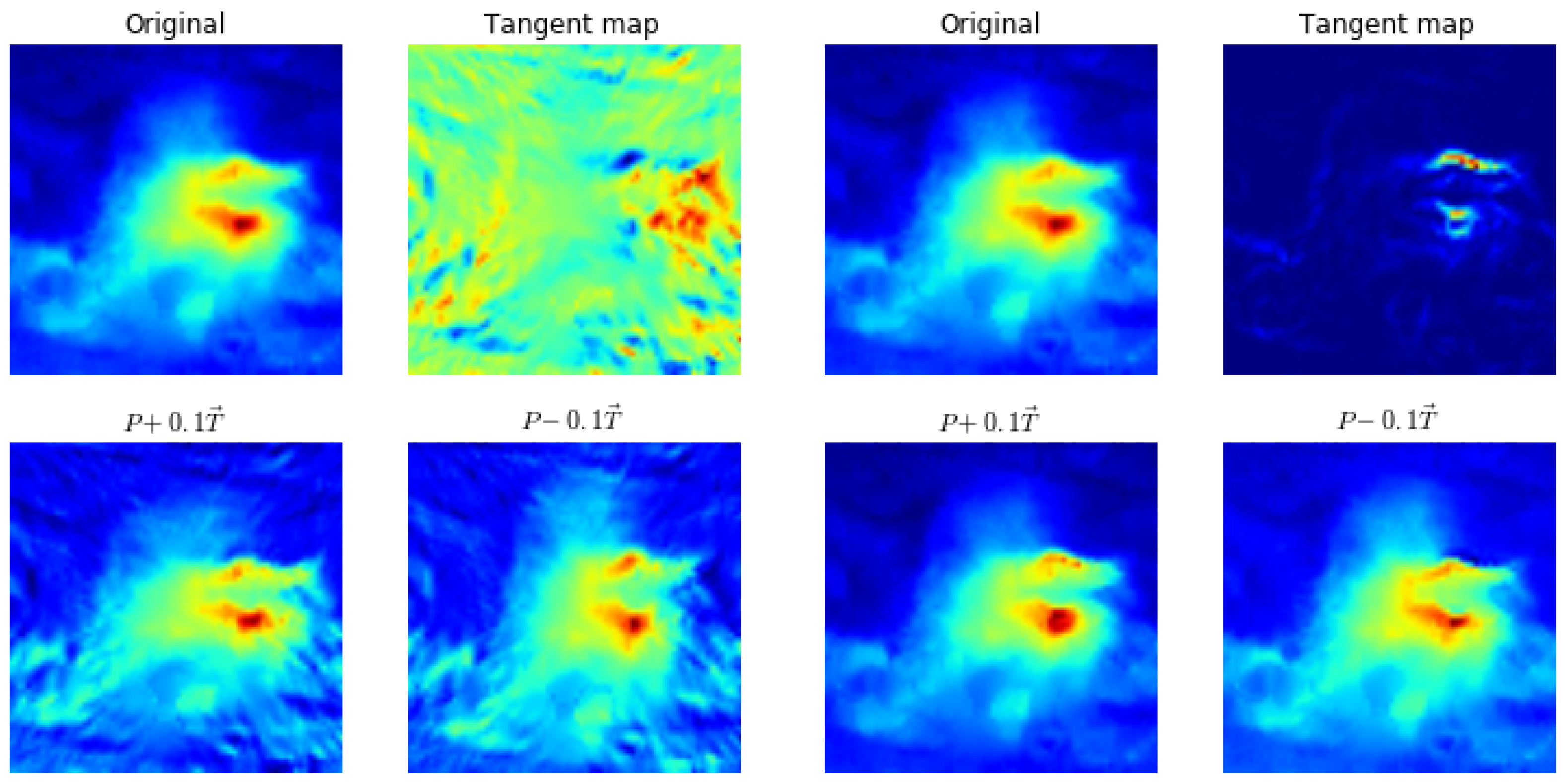
Rotation manifold (left group) ; and thickening manifold (right group) at “2016-01-19 10:30:00”.
Figure 5.
Rotation manifold (left group) ; and thickening manifold (right group) at “2016-01-19 10:30:00”.

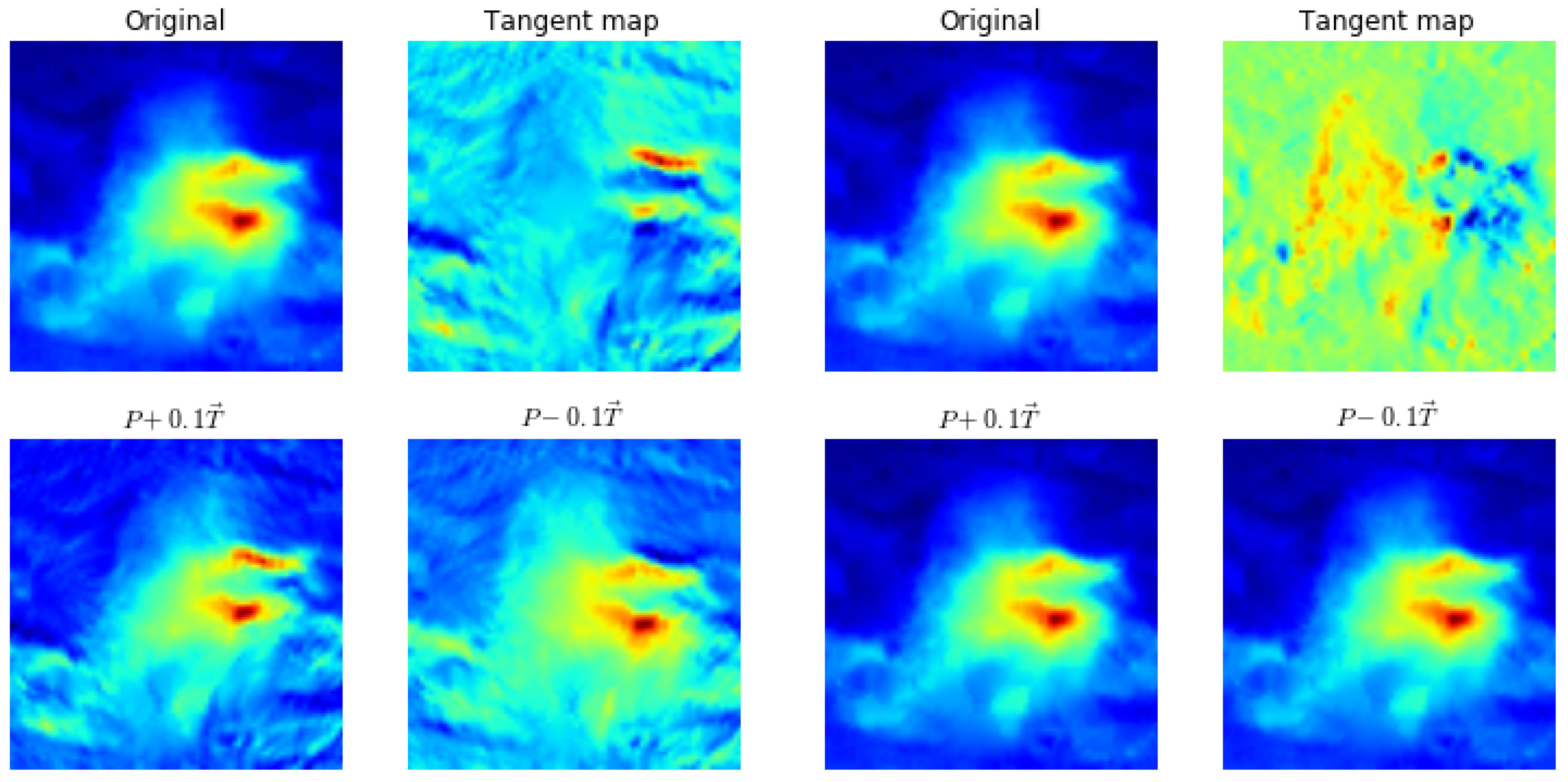
Figure 6.
Scale transform (left group); and Y-translation (right group) at “2016-01-19 10:30:00”.

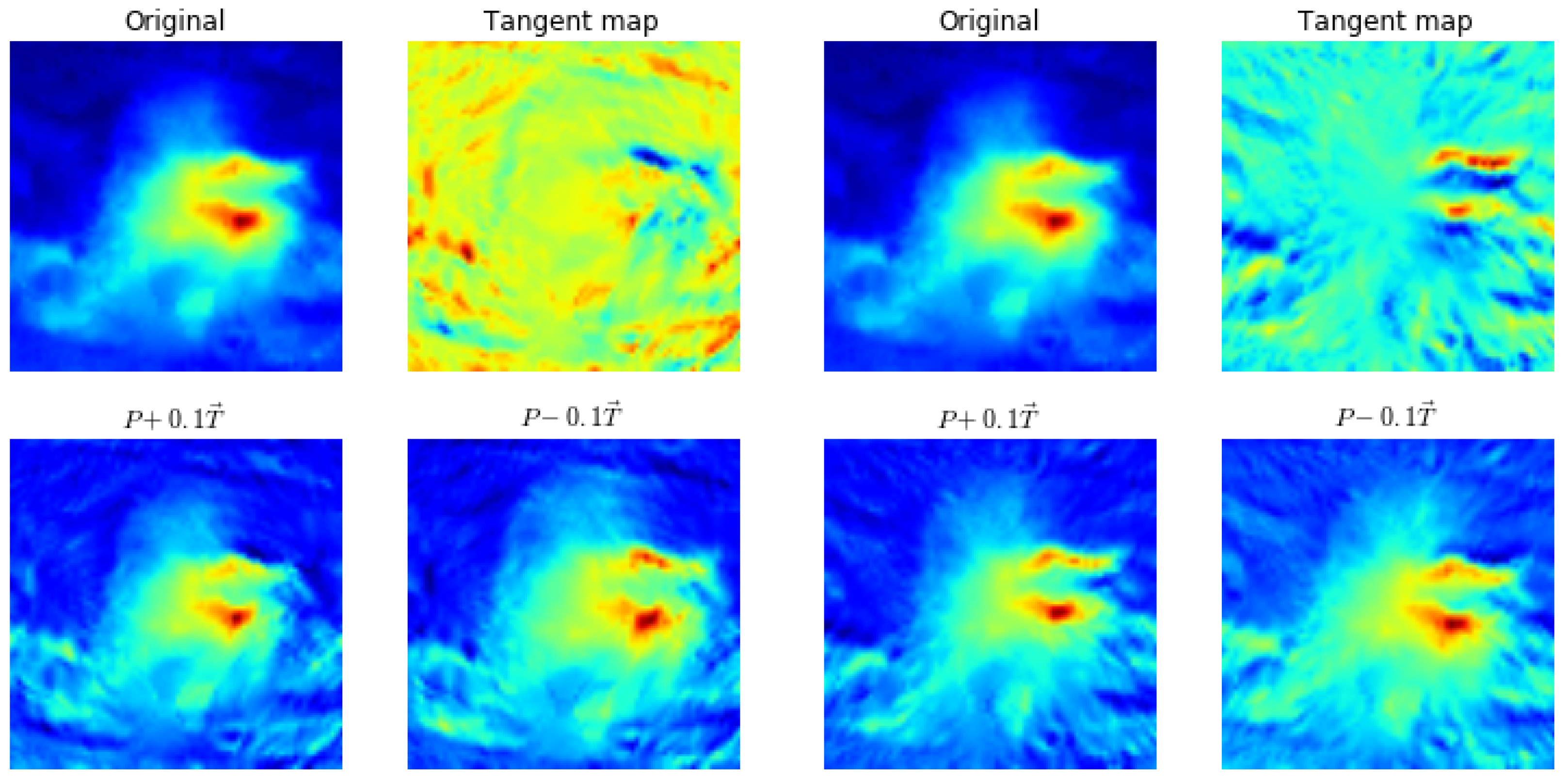
Figure 7.
Diagonal hyperbolic transform (left group); and parallel hyperbolic transform (right group) at “2016-01-19 10:30:00”.
Figure 7.
Diagonal hyperbolic transform (left group); and parallel hyperbolic transform (right group) at “2016-01-19 10:30:00”.

Figure 8.
Forecasting at a horizon of 3 h (Tangent space method), at time stamps, 2016-05-12 15:15:00 (left group) and 2016-02-21 13:15:00 (right group). For each group, we plot: current map ( upper left); target map () (upper right); prediction error (lower left); and forecast ( lower right).
Figure 8.
Forecasting at a horizon of 3 h (Tangent space method), at time stamps, 2016-05-12 15:15:00 (left group) and 2016-02-21 13:15:00 (right group). For each group, we plot: current map ( upper left); target map () (upper right); prediction error (lower left); and forecast ( lower right).

Figure 9.
Weights for a one hour forecast at time “2016-02-21 13:15:00”. The term , indicates the tangent space and the corresponding time lag.
Figure 9.
Weights for a one hour forecast at time “2016-02-21 13:15:00”. The term , indicates the tangent space and the corresponding time lag.

Figure 10.
Time evolution of the TEC RMSE, for the case of forecast with the tangent space method (red), and frozen map method (blue) for different horizons (see annotation on the upper part of the figures).
Figure 10.
Time evolution of the TEC RMSE, for the case of forecast with the tangent space method (red), and frozen map method (blue) for different horizons (see annotation on the upper part of the figures).

Figure 11.
Box plot of the TEC RMSE, for the case of forecast with frozen value (left) and the tangent space (right), for each horizon (see the tick labels of each figure).
Figure 11.
Box plot of the TEC RMSE, for the case of forecast with frozen value (left) and the tangent space (right), for each horizon (see the tick labels of each figure).

Figure 12.
Histogram of the forecast RMSE ratio between the tangent space method, and a frozen map method: (Upper left) horizon at 30 min; (upper right) horizon at 1 h; (lower left) horizon at 3 h; and (lower right) horizon at 24 h. From 2016-01-10 to 2016-02-21, a total of 4080 maps.
Figure 12.
Histogram of the forecast RMSE ratio between the tangent space method, and a frozen map method: (Upper left) horizon at 30 min; (upper right) horizon at 1 h; (lower left) horizon at 3 h; and (lower right) horizon at 24 h. From 2016-01-10 to 2016-02-21, a total of 4080 maps.

Figure 13.
Time evolution during a whole year of the total RMSE in TECUs for a horizon of 3 h: (Left) the frozen forecast, with in red the time series low pass filtered; and (Right) the forecast by means of the tangent space method.
Figure 13.
Time evolution during a whole year of the total RMSE in TECUs for a horizon of 3 h: (Left) the frozen forecast, with in red the time series low pass filtered; and (Right) the forecast by means of the tangent space method.

Figure 14.
RMSE of tangent space method (left) vs. RMSE of frozen map method (right) as a function of the latitude.
Figure 14.
RMSE of tangent space method (left) vs. RMSE of frozen map method (right) as a function of the latitude.

Figure 15.
Root Mean Square in TECUs as function of the latitude (left). Ratio of RMSE the Tangent Distance Forecast Error to the Frozen forecast error (right).
Figure 15.
Root Mean Square in TECUs as function of the latitude (left). Ratio of RMSE the Tangent Distance Forecast Error to the Frozen forecast error (right).

Figure 16.
Decomposition of the forecast error variance “ (left) vs. Bias (right). Note that the units are .
Figure 16.
Decomposition of the forecast error variance “ (left) vs. Bias (right). Note that the units are .

Figure 17.
Normalized log frequency histogram of the forecasting RMSE.


Table 1.
List of time lags and weights in the forecasting model. Note that the subindex “d” runs along all the tangent spaces listed in .
Table 1.
List of time lags and weights in the forecasting model. Note that the subindex “d” runs along all the tangent spaces listed in .
| State | Output | Input 0 | Input 1 | Input 2 | Input 3 | Input 4 | Input 5 |
|---|---|---|---|---|---|---|---|
| Training | h | h | h | ||||
| Forecasting | h | h | h | ||||
| Weights | , | , | , | , | , | , |
Table 2.
Ratio of the RMSE between tangent space forecast and frozen maps wrt actual maps for different horizons.
Table 2.
Ratio of the RMSE between tangent space forecast and frozen maps wrt actual maps for different horizons.
| Horizon | 1/2 h | 1 h | 2 h | 3 h | 6 h | 24 h |
|---|---|---|---|---|---|---|
| Ratio | 84.99% | 77.65% | 71.35% | 69.34% | 87.23% | 95.76% |
Table 3.
Improvement Ratio of the RMSE between tangent space forecast and frozen maps when using the tangent space forecaster vs. the case of not using the tangent space of each of the maps.
Table 3.
Improvement Ratio of the RMSE between tangent space forecast and frozen maps when using the tangent space forecaster vs. the case of not using the tangent space of each of the maps.
| Horizon | 1/2 h | 1 h | 2 h | 3 h | 6 h | 24 h |
|---|---|---|---|---|---|---|
| Ratio Tang Space method | 84.99% | 77.65% | 71.35% | 69.34% | 87.23% | 95.76% |
| Ratio using Maps only | 89.08% | 80.90% | 76.95% | 73.07% | 91.45% | 94.08% |
| Ratio DCT Method | 87.75% | 78.25% | 74.38% | 71.21% | 88.94% | 89.11% |
Table 4.
Empirical fraction of values greater than a TECU value.
| TECU | 2 | 4 | 6 | 8 | 10 | 12 |
|---|---|---|---|---|---|---|
| Prob ( > TECU ) |
© 2018 by the authors. Licensee MDPI, Basel, Switzerland. This article is an open access article distributed under the terms and conditions of the Creative Commons Attribution (CC BY) license (http://creativecommons.org/licenses/by/4.0/).
Share and Cite
MDPI and ACS Style
Monte Moreno, E.; García Rigo, A.; Hernández-Pajares, M.; Yang, H. TEC Forecasting Based on Manifold Trajectories. Remote Sens. 2018, 10, 988. https://doi.org/10.3390/rs10070988
AMA Style
Monte Moreno E, García Rigo A, Hernández-Pajares M, Yang H. TEC Forecasting Based on Manifold Trajectories. Remote Sensing. 2018; 10(7):988. https://doi.org/10.3390/rs10070988
Chicago/Turabian StyleMonte Moreno, Enrique, Alberto García Rigo, Manuel Hernández-Pajares, and Heng Yang. 2018. "TEC Forecasting Based on Manifold Trajectories" Remote Sensing 10, no. 7: 988. https://doi.org/10.3390/rs10070988
Note that from the first issue of 2016, this journal uses article numbers instead of page numbers. See further details here.