On-the-Fly Olive Tree Counting Using a UAS and Cloud Services


Computer Architecture Department, UPC BarcelonaTECH, Esteve Terrades 7, 08860 Castelldefels, Spain
*
Author to whom correspondence should be addressed.
Remote Sens. 2019, 11(3), 316; https://doi.org/10.3390/rs11030316
Submission received: 18 January 2019
/
Revised: 2 February 2019
/
Accepted: 3 February 2019
/
Published: 5 February 2019
Abstract
:Unmanned aerial systems (UAS) are becoming a common tool for aerial sensing applications. Nevertheless, sensed data need further processing before becoming useful information. This processing requires large computing power and time before delivery. In this paper, we present a parallel architecture that includes an unmanned aerial vehicle (UAV), a small embedded computer on board, a communication link to the Internet, and a cloud service with the aim to provide useful real-time information directly to the end-users. The potential of parallelism as a solution in remote sensing has not been addressed for a distributed architecture that includes the UAV processors. The architecture is demonstrated for a specific problem: the counting of olive trees in a crop field where the trees are regularly spaced from each other. During the flight, the embedded computer is able to process individual images on board the UAV and provide the total count. The tree counting algorithm obtains an score of for a sequence of ten images with 332 olive trees. The detected trees are geolocated and can be visualized on the Internet seconds after the take-off of the flight, with no further processing required. This is a use case to demonstrate near real-time results obtained from UAS usage. Other more complex UAS applications, such as tree inventories, search and rescue, fire detection, or stock breeding, can potentially benefit from this architecture and obtain faster outcomes, accessible while the UAV is still on flight.
1. Introduction
Currently, many precision agriculture works are using UAS due to their flexibility and low price [1,2,3,4,5]. Usually, the UAV flies over the field of interest collecting the aerial images. The flight time ranges from several minutes to hours, depending on the type of UAV and the area to be covered, among other factors [6]. When using short-endurance UAV, several take-offs and landings may be needed. The operator of the UAV is able to manually check the correctness of the sensing by downloading some low-resolution images to the ground or during the technical stops. The high-resolution images are stored in the memory card of the camera. Once the aerial work is finished, they are transferred to a computer for post-processing. Software such as Pix4Dmapper [7], Correlator3D [8], or Agisoft PhotoScan [9] are used to generate a mosaic where all the images are stitched together thanks to a generous overlapping (60–80%) [10]. Although available, the autopilot telemetry is seldom used during this post-processing.
The complexity of image processing algorithms [11] and the large number of images taken in a single aerial work (around thousands) foster the need for powerful computing resources. Thus, this post-processing must be done at the UAV operator’s premises using computers with significant amounts of memory, powerful co-processors, or computer clusters [12]. The whole process might easily take about 2–3 days to finish, with the inconvenience that this elapsed time supposes for the end-user. In a survey paper of thermal remote sensing applied to precision agriculture [13], the delivery time was considered even higher (approximately from 1–3 weeks). As an example, a regional mosaic created from two gigabytes of data took 25 h of processor time when no parallelism was applied [14]. Furthermore, in [15], the authors related a long time (about 20 h) to process a set of multispectral images (about 100) captured with a UAV. The authors used a commercial software executed on a powerful computer (a 12-core Intel i7 processor and 64 GB of RAM) for creating orthomosaics at ultra-high resolution (14.8 cm per pixel).
In this work, we propose a new architecture and procedure with the purpose of delivering useful information to the end-users during or immediately after the flight. The data processing used to demonstrate the contribution is the specific problem of detecting trees and counting them in a large field. Although this problem may seem artificial for a crop, it may be useful when the crop is a very large extension, or in cases of agriculture public subsidies, if paid per tree, or at the moment of transferring to a new owner. Moreover, a similar and well-known problem, such as counting people in a crowd, can benefit directly from this proposed architecture. For this, we propose adding an embedded computer, such as an oDroid board [16] or a RasberryPi computer [17], to the UAV. In the future, when more computing power will be available onboard the UAV, the proposed architecture can be used to create more complex outcomes such as orthomosaics or cloud point maps.
In the proposed architecture, the embedded computer processes the images on-the-fly and sends only the relevant findings to the ground station. Upon receiving these relevant data, the ground station can easily map the results as an overlay on a state-of-the-art geographical information system. Assuming the ground station has an Internet connection available, the results can be uploaded to the cloud almost instantly to be shared with the end-user. The purpose of orchestrating all the hardware in such a computing hierarchy (UAV/ground station/cloud) is the very fast delivery of the final product to the client.
2. Background
Remote sensing using UAS is today a reality. They are becoming a useful tool, especially in non-populated areas, for forestry and agriculture. In many works, UAS are used in agriculture to obtain the irrigation status or fruit maturity, thus informing decisions on watering or harvesting. An inventory work using a UAV was presented in [18] for the timely detection of weeds on cotton and sunflower plantations. 3D reconstruction of the parcels provided the height of the plants as an additional feature for a random forest classifier. Using commercial off-the-shelf payload, [19] related how a UAV with an RGB camera is used for the inventory of trees in a nursery of plants. A similar target was addressed in [20] using stochastic geometry algorithms and in [21] using neural networks, where a UAV flying between rows of fruit trees was tested to recognize the fruits (apples and oranges). Palm tree counting from RGB images was addressed in [22] by integrating template matching and object-based image analysis.
More complex scenarios are found by UAV flying over forest, having as the target the monitoring, classification, or inventorying of the vegetation of wild areas. For instance, [23] classified three species of trees using high-resolution airborne hyperspectral imagery or [24] also using an airborne laser scanner. LiDAR sensors were the only device used for a similar task of another tree classification work [25] and in the review of tree segmentation methods presented in [26]. In [27], the authors used a UAV with a high-resolution camera modified to detect infrared bands and 3D reconstruction methods to calculate the altitude of the tree crowns. In [28], the authors investigated the possibility of automatic individual tree detection from the canopy height models (CHMs) that can be derived using structure-from-motion (SfM) algorithms on RGB photographs, similar to the process using LiDAR-derived CHMs. In [29], the authors flew above 11 locations in Finland with the aim to classify forest trees. The species to differentiate were pine, spruce, birch, and larch. They had 56 experimental plots with 4151 reference trees, which were used as the ground-truth for the experiment. The sensors used on board the UAV included a spectrometer, a LiDAR, a high-resolution RGB camera, an irradiance sensor, and a Fabry–Pérot interferometer. Up to 347 different features were available and used all together or in groups by sensor, as well as different classification algorithms (naive Bayes, decision trees, K-nearest neighbors, random forest, and multilayer perceptron) and different performance metrics (accuracy, recall, precision, F1-score and Kappa) to assess which options are most adequate. The processing needed some manual interaction, e.g., related to the ground control points, and required a long time for computation. An extensive review of tree species classification methods can be found in [30].
A comparative work [31] used six different algorithms to detect individual trees in areas of three different European countries, based on infrared sensors. Six isolated aerial images with an infrared band for diverse areas (dense forest, sparse forest, and tree plantation fields) were used as test inputs of the algorithms. The ground-truth was derived from four independent humans and set as the average of the tree crown locations. The algorithms used a number of image processing methods and statistical filters. In all the algorithms tested, the best results were obtained for the image showing a plantation of trees, due to the ease of background separation between plants with a matching score of with four human interpreters.
The detection of individual trees, not of their species, was the target of other previous works [32,33,34]. Given the complex environment of trees in a forest, most authors mainly use hyperspectral cameras and LiDAR or laser-scanner sensors to build photogrammetric point clouds and count the dominant tree crowns. Onishi and Ise [35] used a UAV and its RBG images to train a deep learning algorithm to detect individual trees and classify them. They reported many-to-one segmentation errors that needed to be corrected manually. Additionally, UAV’s remote sensing capabilities have been used to detect and segment trees deteriorated by myrtle rust in natural and plantation forests [36]. This work illustrates an experimentation case on paperbark tea trees in Australia, which integrates an on-board hyperspectral camera and several machine learning algorithms for the classification. Once trained, the system proved to be very accurate and efficient in classification, with a global multiclass detection rate of , but requiring about 3 min to evaluate every new instance. All of these works focus more on the scientific aspect and on the quality of the results than on the time-to-delivery challenge.
The processing of [29] for the trees classification of each single location, flown over for 10–30 min, needed between 22 h to more than 50 h of processing at the researcher’s premises. In [18], the authors related a complex pipeline of algorithms, known as object-based image analysis, which ended with a final map of the areas with weeds. It needed 40 h of processing using commercial software. Most of the classification and segmentation algorithms used on the UAV were initially tested in fixed cameras. For instance, people detection and counting is a recurrent topic in many research works [37,38,39].
With the continuous increase in the number of aerial devices being used (satellites, constellations, pseudo-satellites, airborne UAV, and balloons) and of the number of deployed on-site sensors, the storage needed was approximated to exceed one exabyte (one thousand petabytes or one million terabytes) in 2014 [12]. The authors presented the new challenges created by this incremental rise of remote sensing data. Big data infrastructures and processing capabilities need to be applied to next-generation remote sensing applications to convert these data into useful information. The work in [40] addressed the different parallelization strategies for processing the high quantity of data at different architecture levels, including virtualization, cloud computing, grid computing, service-oriented architectures, or specific hardware and multicores. Moreover, it addressed the new trends in remote sensing developments, which have been dictated mainly by government intelligence and scientific agencies, but also by more general users and companies. For new users, time to market is an important cost, and reduction of costs is a must. As an example, AgrCloud [41] is a proposed solution for providing remote sensing processing services through the Internet, able to obtain speed-ups of two-timesusing the MapReduce paradigm in a four-node cluster. The potential of parallelism as a solution in remote sensing has never been addressed for a distributed architecture that includes the UAV processors.
Cloud computing is a paradigm that arises from the expansion of services available on the Internet. Initially available as remote disk space, cloud services started to evolve into virtual computer services, parallel computing clusters, and specific software execution sites. Concepts such as platform as a service, software as a service, elastic computing, etc., began to appear to describe all of these services. They are all part of cloud computing and are provided through the Internet, with the actual location of the hardware being irrelevant. Recently, the term cloud-assisted remote sensing has been proposed to expand the cloud services to remote sensing applications, creating the new concept of sensing as a service [42]. Its main advantage is the possibility to share data collected remotely with many users and in real time. For instance, eco-monitoring (http://research.engr.oregonstate.edu/ecomonitoring) shows the web users, in real time, images with the status of some agriculture crops. These works show the potential of the Internet for remote sensing, but are still too generic and not end-user-oriented.
3. Materials and Methods
This paper presents remote sensing as an Internet service, using a UAS for a simple tree counting case. We use the images captured during a flight over a field of olive trees in Andalucia, Spain, with the objective of counting the number of olive trees in it. We show how to process the images one by one, as they are captured by the camera. A RaspberryPi [17] was used to demonstrate that the information relevant to the end-user can be obtained during the flight. The requirements are that the counting will be computed and delivered in real time, while flying, and that the final value has an accuracy similar to that obtained by the post-processing of the mosaic.
3.1. Study Area and UAV Description
The test field is a crop of almost 50 ha that crosses the border between Málaga and Sevilla provinces in Spain. The area under study has an average elevation of 540 m, and the terrain slope is between and . Young olive trees have only one crown and are 7 m apart. Some parcels also have old trees. Old olive trees generally have 3 crowns and are 13 m apart, but we found trees with 4 crowns and separated by shorter distances. There is no official count of the number of trees, just an approximate density measure of 204 of young trees per hectare (59 trees/ha for the older trees). Figure 1 shows the plot of the crop.
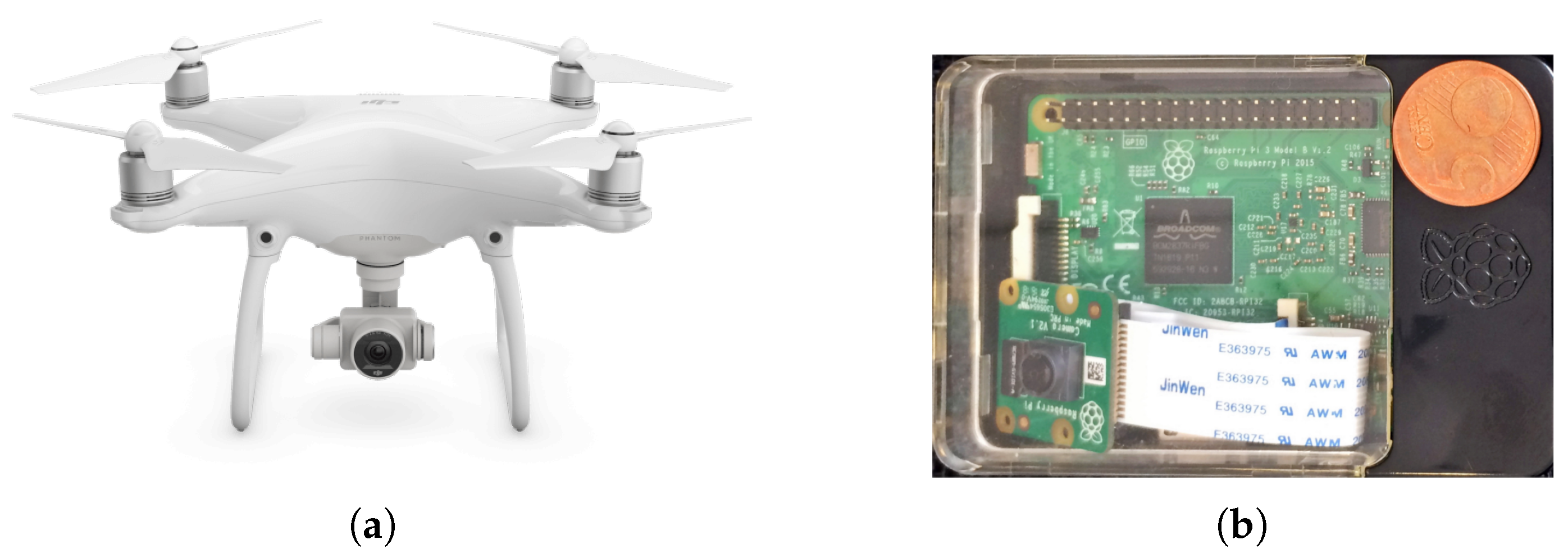
Images were taken with a DJI Phantom4 (see Figure 2a). This is a small light-weight UAV (35 cm and 1.380 g) with a front camera for obstacle avoidance and a second camera integrated in a gimbal as the payload. This camera can take images at 20 Hz and store them in a micro SD. Available formats are either JPEG or DNG (raw). The camera can also be set to record video instead of photographs. Images or videos can be downloaded to the ground at 30 fps, but only with low resolution (0.69 megapixels). This speed is enough for a video-streaming visualization, but not for the image processing. For this flight, the camera was set to capture images of 12 megapixels (4000 × 3000) in size at time intervals of 2 s. Figure 2b shows the proposed payload processing board, a RaspberryPi, with the camera incorporated. This board has been used for the evaluation of the execution time of the algorithms.
While transmitting high-resolution images is very bandwidth consuming, processing the images on board, before sending just a list of trees, is a very economic solution: both the bandwidth required and the power consumption for the transmission are two orders of magnitude less than the full image. The latitude and longitude of a tree (two floats) for approximately 80–140 trees per image makes the total size close to 1 KB of data. Sending 1 KB of data to the ground every 2 s can be achieved using the command-and-control (C2) channel without compromising it. Alternatively, using another communication channel for the payload, such as a WiFi, WiMax, or a broadband mobile connection, permits the use of the C2 link exclusively for the flight control and increases the safety of the flight. In our architecture, we decided to use a separate WiFi channel for the payload to avoid interference with the C2 link and also because in rural areas, the broadband cellular network is not always available. The use of the WiFi link has as a disadvantage the limitation of the communication range to a distance of 250 m in radius. This limitation can be overcome with the use of a delay-tolerant networks protocol [43].
Another decision made in relation to the communications architecture is that the broadband mobile connection to access the Internet cloud is done from the ground station and not from the UAV. The advantages of this decision are the following: The best location of the ground station can be decided in advance and checked before flight, which will permit a continuous connectivity with no disconnections. Furthermore, by sending all the data first to the ground station, the human remote pilot can check that the software is executing correctly. Finally, all forwarding of data to the cloud, if needed due to the weak signal of the available broadband communication network, is done by the ground station, which is the less power-critical part of the system.
3.2. Data Processing
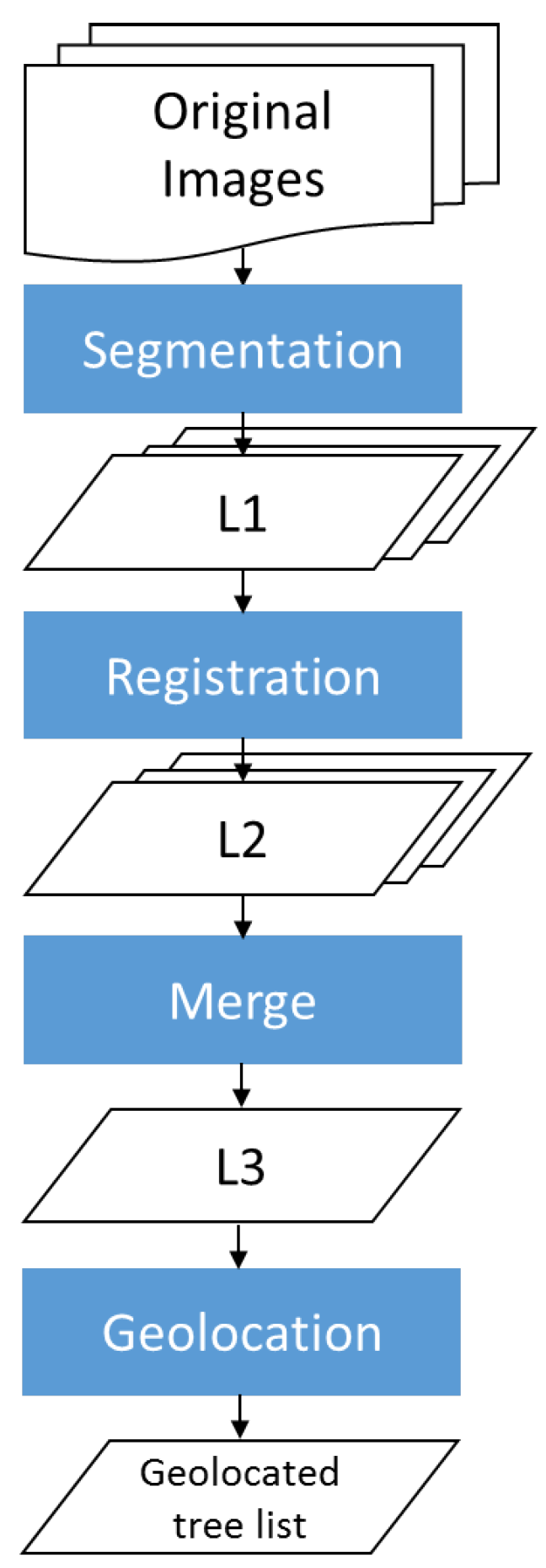
Figure 3 illustrates the data flow of the tree counting application. For each image, the segmentation module detects the olive trees in the image (L1). Then, at the registration and merge modules, the image pixel coordinates are projected to a global reference system (L2), and multiple observations of the same tree are merged (L3). Finally, the geolocation module computes the geographic coordinates of each new tree and sends them to the ground station, so that the results can be visualized in real time. Two different techniques have been tested to detect the olive trees: color-based segmentation and stereo vision-based segmentation.
3.2.1. Color-Based Segmentation
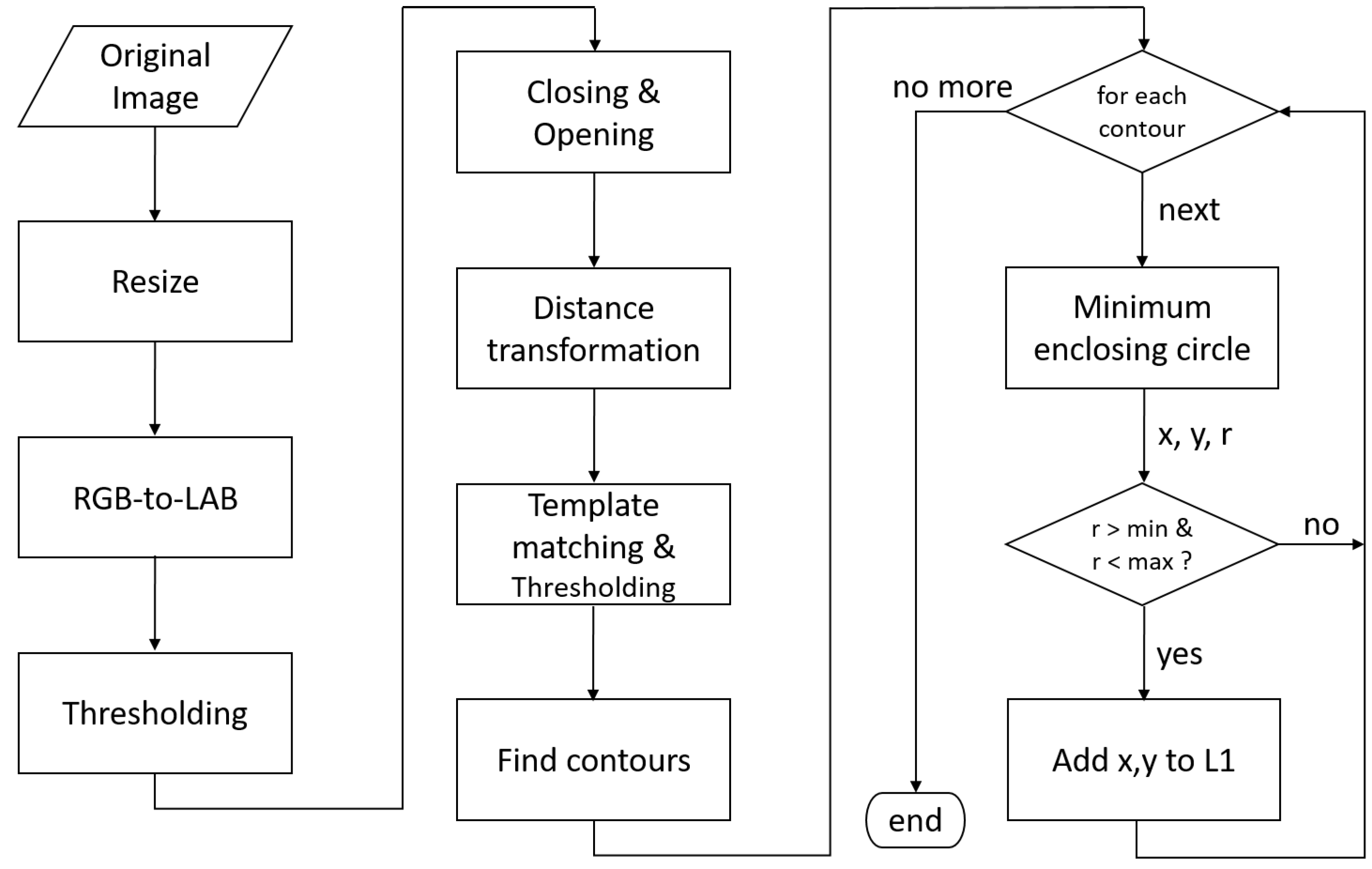
Figure 4 shows the flowchart of the color-based segmentation algorithm. The detail of the processing at intermediate steps for a specific image is given in Figure 5. The image is first scaled both to reduce computational efforts and to put all images to the same scale. Spatial parameters, such as the kernel size in morphological operations or the template size, have been calculated experimentally for an image taken at 100 m of altitude and scaled to 25% of the original size. For each image, the scale factor s is calculated depending on its flight altitude h above ground level (AGL) ().
The images are next converted from the original RGB (red/green/blue) to the CIE Lab color space. Previous literature [44] has shown that the RGB images are not the most convenient representation for the soil/plant classification problem. After comparing 11 different color spaces on a set of images, the CIE Lab color space was shown to achieve superior classification with the a channel producing a 99.2% accuracy. The CIE Lab color space consists of one luminance channel (L) and two chrominance channels (a and b). The a axis extends from green to red and the b axis from blue to yellow. Minimum () and maximum () thresholds have been defined for the olive trees in the CIE Lab color space based on the values of the pixels in the tree areas and compared to the background and to other vegetation that could be found in the images.
After CIE Lab channels, thresholding, closing, and opening morphological operations with a kernel of size 3 × 3 are applied on the resulting binary image to remove noise (Figure 5a). Considering that we are looking for circular shapes, we compute the distance transform, where the value of each pixel is replaced by its distance to the nearest background pixel (Figure 5b), and use template matching to search for matches between the distance image and a disk template (Figure 5c). The template has been designed taking into account the usual values of size and separation between olive trees. The used template is the result of applying the distance transform on a white circle of 30 pixels in diameter centered on a black square of size 80 × 80 (top left corner in Figure 5b). The resulting image is filtered using Otsu thresholding [45] to obtain the peak regions, each corresponding to an olive tree. Finally, the minimal enclosing circle of each region is computed to obtain the center coordinates and the radius (Figure 5d). Only circles with a radius between 5 and 45 pixels size are returned as trees. The algorithm returns a list containing the pixel coordinates of the center of the trees.
3.2.2. Stereo Vision-Based Segmentation
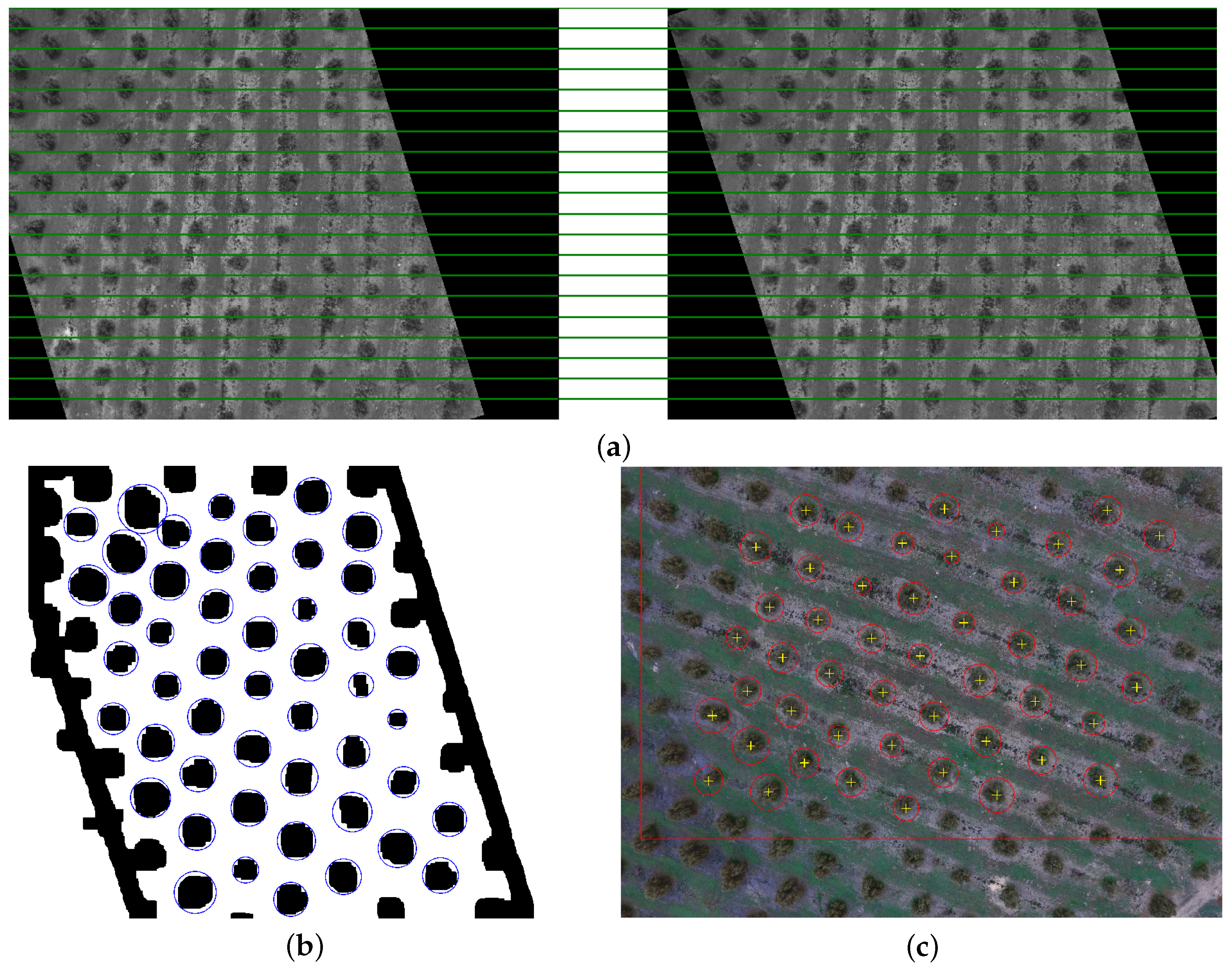
In every pair of consecutive aerial images, we have two different views of the same but displaced scene. Stereo vision consists of using these two views to obtain information about the distance of the objects in the scene to the cameras. The two views, after being projected on a common plane using the epipolar geometry, will have the same trees in the same horizontal line (see Figure 6a). Then, by comparing the distances between pixels corresponding to the same object, the depth information can be calculated using well-known algorithms [46]. The disparity map is a new generated image in which pixel values are inversely proportional to the depth of the scene. Hence, high value pixels belong to objects closer to the cameras. Analyzing these disparity maps will allow us to locate separate trees on them.
Image rectification is the process of projecting two images of the same scene on a common plane. Two consecutive images are taken, and common keypoints are located by a feature-matching algorithm using SURF [47]. Based on the keypoints matching, homography matrices are calculated for both images. Semiglobal matching [48] was used to produce the disparity map from two rectified images. To obtain the information about separate trees from the disparity map, two more steps are required: separating trees from the ground and detecting trees in the resulting image. To separate trees from the ground, we tested the adaptive threshold and the median filter algorithms [49]. While they produced similar results, the adaptive threshold was much faster. To detect each separate tree, we used the contour detecting algorithm [50] (see Figure 6b).
The result of stereo vision-based segmentation can be seen in Figure 6c. Yellow crosses and red circles show the detected trees. The straight red lines delimit the overlapping area of this image with its peer image in the stereo pair. As expected, the part of the image with no overlap has no trees detected. This is because of the lack of stereo information for it. With the exception of the first image, these omissions will be recovered by processing the successive pair of images as explained in the next Section 3.2.3; thus, we do not consider them as a problem. On the contrary, when observing the overlapping area, we found more undetected trees. As shown in Figure 6b, the trees close to the borders are also not captured by the adaptive threshold. Other undetected trees are due to the implementation details of the process of rectification, which loses some parts of the image close to the corners.
3.2.3. Registration and Merge
During the UAV flight, the camera is configured to take a picture at a fixed time period (one every 2 s). Each image separately goes through the segmentation process described above and results in a list of pixel coordinates. When the segmentation algorithm processes the following image, it obtains a new list of pixel coordinates. Given the overlap of the images (80%), many trees located in the first image will appear in the subsequent images. In order to detect which trees are new and which are repeated, we need to project the image pixel coordinates to a global reference system and detect which observations correspond to the same tree. This process is repeated for each new image captured by the camera on board the UAV. The processing flows involved are shown in Figure 7.
Every new image is paired with its previous image using a classical feature detection and matching algorithm (Figure 7a). For each pair of sequential images (let us name them as and ), ORB features are computed and matched to calculate the homography matrix . Applying the matrix to the pixels of would project them onto the same plane as image . Every new matrix is composed with the previous in order to have all tree locations related to the first image reference system. In this way, the upper-left pixel of the first image is the origin of the global reference system, and applying the same process consecutively to each new image in the stream, all the image pixel coordinates () are converted to global coordinates (). Notice that the perspective transform does not need to be applied to all the pixels in the image, but only to the locations of the trees.
It is expected that the same tree can appear in more than one image, but with slightly displaced coordinates. We use a fixed-radius nearest neighbor search [51] to recognize previous observations of the same tree and avoid duplicates. The list of trees of the first image is used to populate the initial global list (). For each new image, its list of trees is merged into following the processing flow in Figure 7b. First, a kd-tree search structure is built from the set of tree locations in . For each tree in the new , we search for the nearest neighbor inside a fixed radius bound. If there is no neighbor on that radio, it means that there is no previous observation of that tree, and the location is added to as a new tree. Otherwise, it means that the tree already existed in , and the new observation is merged with the already existing global tree, thus avoiding counting it twice or more.
3.2.4. Geolocation
The ultimate goal of the UAS application is to count the total number of olive trees and obtain the geographic coordinates of each tree. Each image is tagged with the position and attitude of the UAS at the time it was taken. We use direct georeferencing [52] to compute the tree’s coordinates without the use of control points or aerial triangulation. It takes into account the effects of terrain elevation and slope using an iterative algorithm. Initially, the elevation of the target is estimated as the terrain elevation in the vertical plane of the UAV, and a first estimation of the coordinates is computed. Based on the estimated coordinates, a new possible value of the terrain elevation is obtained and used for the next iteration. For this, the digital elevation model (DEM) of the area is needed. The DEM file can be obtained from the national cartographic services (http://centrodedescargas.cnig.es). The file size is 1.4 MB, and its content is a matrix with the corresponding elevation of the terrain on each cell with a resolution of 5 m per cell. These data are uploaded to the payload computer in advance to enable the on-board processing.
3.3. Data Presentation
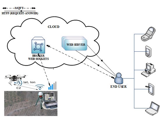
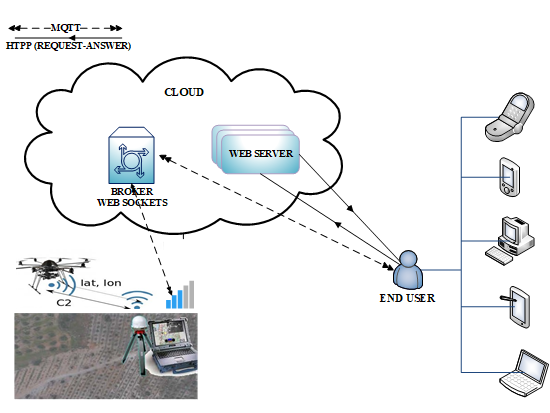
The immediate delivery of final output to end-users is achieved by building a data stream network architecture similar to the one used for the Internet of Things [42,53]. The solution assumes that the end-users can be anywhere on Earth as long as they have an Internet connection through a laptop or any other personal device. With a data stream network architecture, they will be able to receive the final product in almost real-time. Moreover, they will visualize the trees over a map using a user-friendly interface, interact with the visualization, and all this without having to install any software, just using the browser.
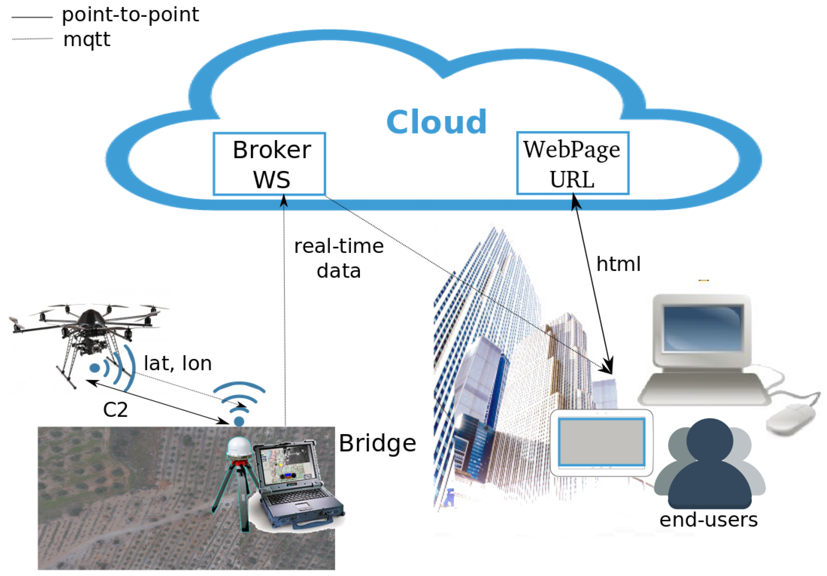
The architecture used is shown in Figure 8. The UAV has a very light and inexpensive on-board computer (e.g., a RaspberryPi), which receives the image sequence and executes the algorithms presented above. Each time a new image is processed, the global list of the trees is updated. Given the high level of overlap between an image and the following one, the number of new trees detected will occupy less than 1 KB of data. Their locations, once converted to lat/lon coordinates, are sent to the ground station. The ground station will store the information, but also will stream it to the cloud. The mqtt protocol, together with a broker such as mosquitto, is used for this task [54]. The mqtt protocol is a text-based protocol, which consumes very little bandwidth and is used extensively in the Internet of Things and smart cities research works. For instance, in [55], mqtt was used to build a context-aware data model for smart cities, such as crowd monitoring (counting people in an area) or environmental information (pollution, air quality, temperature, humidity, noise, etc.). The protocol is built for low-consumption devices and allows encryption and different levels of quality of service.
The UAS data publisher is provided by a running computer available in the cloud. This computer holds a web page with a WebSocket [56]. For the web page, we selected the classical web architecture with JavaScript, HTML, and CSS, to which we provided a dynamic functionality using Node.js. Attached to the WebSocket, we set up a mqtt broker.
The flow of data is as follows: For each image, the UAV creates a new stream of data, containing the locations of the new detected trees. This is a short text message, which is sent to the ground station through the light weight protocol. The ground station runs a mqtt bridge, and all the data that arrives through the WiFi channel are forwarded to the broadband channel. The destination is the mqtt broker, which uses a public WebSocket to receive the data and retransmit them to all subscribers of the service.
On the other side, from anywhere and at any moment, any person with the web page address can connect to it. When the HTML code of the web page is downloaded on the end-user’s device, the JavaScript code executes and connects automatically to the WebSocket, subscribing to new data. When available, the end-users will immediately receive the data directly on their devices. If the UAV has not yet flown, the page will contain an empty map of the area. If the UAV flight has been completed, all the trees will be shown. If the user connects during the flight, the trees already detected will be in the map by using cloud persistent data. The new ones will appear as soon as detected and published. Further queries could be also programmed to provide access to the available data (i.e., the size of the tree) if the end-user requests it.
3.4. Performance Metrics
In order to validate the results, we manually annotated a sequence of 10 images. We compared the trees detected by the application with the reference ground-truth to obtain the number of true positives (TP or correct detections), the number of false positives (FP or false alarms), and the number of false negatives (FN or detection failures). Notice that the number of true negatives (TN) is irrelevant in this application, since there is nothing to count other than trees; thus, the detection of no-tree objects is not within the scope of this study.
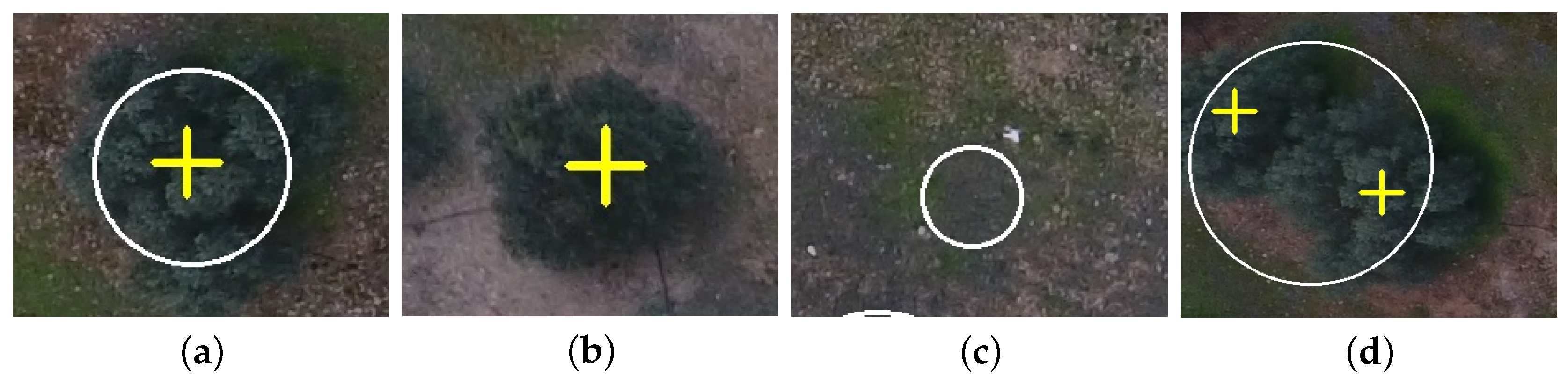
In object detection, this matching between the ground-truth and the detection is not binary in the sense that different ground-truth-to-detection associations can occur [57]: zero-to-one, one-to-zero, one-to-one, many-to-one, one-to-many, and many-to-many (see Figure 9). As our goal is to count trees, if M trees in the ground-truth are associated with one detected tree (as in Figure 9d), we consider TP = 1 and FN = M − 1. In the case that one tree in the ground-truth matches N detected trees, we consider TP = 1 and FP = 1. For the general case M-to-N, where M trees in the ground-truth match N detected trees, we consider TP = , FN = if M is greater than N and FP = if N is greater than M.
Precision, recall, and score are used as classification metrics. Precision, or positive predicted value, indicates the ratio of detected trees that actually shows a correct match with the reference ground-truth (1). Recall, also called true positive rate or sensitivity, measures the ratio of real trees that were correctly detected (2). Thus, high precision indicates a small number of false positives, while high recall indicates a small number of false negatives. The final performance value, the score, is the harmonic mean of the two measures (3).
4. Results and Discussion
4.1. Color-Based vs. Stereo Vision-Based Segmentation
Table 1 shows the tree counts obtained by the color-based and stereo vision-based segmentation algorithms, respectively. The last two rows show the mean absolute error (MAE) and the root mean squared error (RMSE) for each algorithm. The hand-annotated ground-truth column is taken as a reference. This ground-truth is different for the color-based and the stereo vision-based algorithms, since color-based segmentation is able to process the full image, while stereo vision-based segmentation is limited to the overlapping area of consecutive images.
Color-based segmentation clearly outperforms stereo-vision. In the first case, the absolute error ranges from 0–9 trees, with MAE and RMSE below four. On the contrary, stereo vision-based segmentation exhibits excessively large errors, with MAE and RMSE above 30. Furthermore, as we will see below in Section 4.5, the execution time of the stereo vision algorithm is too long and does not allow its execution in real time. Thus, for the global tree count, we decided to discard stereo vision segmentation and use only color-based segmentation.
4.2. Performance of Color-Based Segmentation
Classification performance metrics (TP, FP, FN, precision, recall, and score) of color-based segmentation are shown in Table 2. The numbers in parentheses give the same metrics, but excluding those errors in the detection of trees that are on the edge of the image. The number of discrepancies ranges from zero to a maximum of nine (out of 139) trees, mainly consisting of FN, i.e., undetected trees. Further analysis of the FN shows that most of them (about 68%) come from trees located on the edges of the image. As the next subsection will show, these failures on the edges of the image are solved in the global counter, since they will be detected in the overlapping images. Only two images have FP equal to one, which translates into a precision of near 100%. On average, the algorithm achieves a score of 98.7% (99.5% if borderline errors are not computed).
The worst case is given for image DJI_0232 (shown in Figure 10), where six of the nine failures are due to trees that are on the edge of the image. The three remaining discrepancies are many-to-one associations. These errors occur mainly when the area pattern does not fit the disk template used in the template-matching step, which assumes a circular shape of a given radius and surrounded by a specific space. Thus, the algorithm fails to detect a tree when it is too close to other trees. The work in [22] focused on a similar problem, which is taking stock of the number of palm trees within a plantation. They also highlighted that the template matching algorithm works well in areas where palm trees are separated, but not in dense areas. They found that using object-based analysis is useful to reduce one-to-many errors, but not many-to-one errors. Using template matching and object-based analysis in a subset of the mosaic image, a total of 582 oil palm trees was detected for a ground-truth of 509 trees ( score of 87%). The authors in [28] reported a score of 91%, also counting oil palm trees in a single RGB image with a ground-truth of 184 trees. They used an extreme learning machine (ELM) classifier on a set of extracted SIFT keypoints and local binary patterns (LBPs) to analyze texture information. In [58], a local-maxima-based algorithm on UAV-derived canopy height models achieved a detection of 312 trees for a total of 367 reference trees ( score of 86%) in a forest, which is a far more complex scenario.
4.3. Sensitivity Analysis of the Template Size in Color-Based Segmentation
The selection of the template is related to the shape, size, and separation between olive trees. The trees can be approximated as a circular shape with a variable diameter between 3 and 6 m. The separation between the trees is not constant in all the fields, with values between 7 and 13 m, and different distance separations can also be found in the same image. Moreover, due to the terrain slope, the flight altitude (AGL) is not constant, which makes the tree size and separation in pixels be non-constant. These variations in the scale due to different distance to the ground are resolved in the first step of the segmentation by changing the size of all the images according to their flight altitude, but we can still find areas with trees of different sizes and separations. In the results presented so far, the distance transform over a circle of 30 pixels (about 3.7 m) in diameter centered on a square of size 80 × 80 (about 10 × 10 m) has been used as a template. Table 3 shows the results for less accurate template sizes for image DJI_0232.
As can be observed, decreasing the size of the template causes the appearance of false positives, and the precision drops to 81.4% in the worst case. On the contrary, increasing the size of the template increases the number of false negatives, with a recall of 89.2% in the worst case. The size of the template is related to the separation between trees, while the diameter is related to the size of the tree. If the diameter of the circle is too large, small trees are not detected. Furthermore, two nearby olive trees can be detected as one, causing many-to-one correspondences. Except for the worst case (d = 20 pixels, s = 40 pixels), the score remains over 94% (96% excluding errors in the borderline).
4.4. Tree Counting for a Sequence of Images
The application of the global count algorithm to a sequence of 10 consecutive images reports a total of 330 olive trees, out of the 332 counted by hand, which means an error of in the total count. Classification performance metrics are given in Table 4. As expected, the FN occurring because trees were found too close to the edges are detected in the following overlapping images and become true positives after merging. This leads to an improvement of the recall metric from an average of –. The score that balances the FP and the FN shows very good results (99.09%).
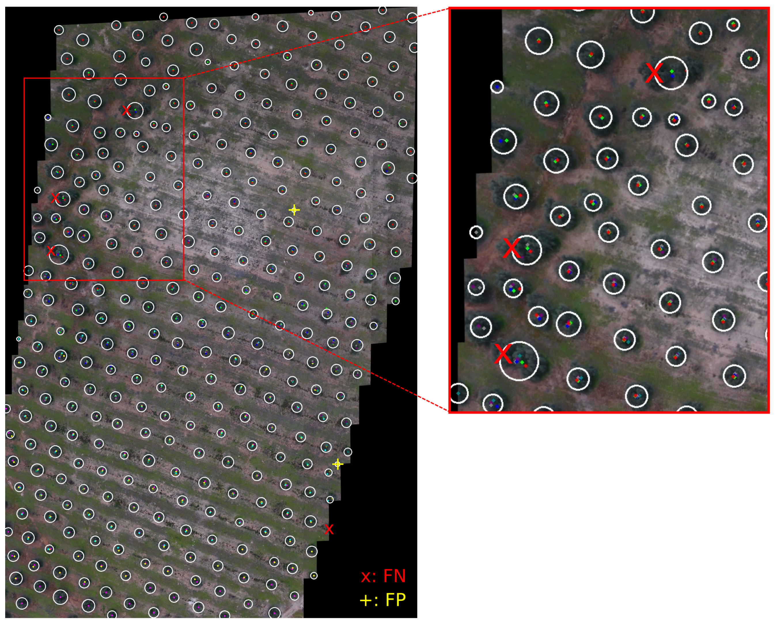
The results for the global count can be validated graphically in Figure 11. Note that this mosaic image was built just for this paper and for algorithm testing, but it is not required during the flight to compute the global tree count. The individually-detected trees are marked using a different color for each image. Thus, a tree detected in four different images shows four different color dots over it. The UAV flight starts from the bottom of the figure and proceeds towards the top. For this reason, we observe that the trees in the bottom rows (belonging to the first image) and the trees in the top rows (from the last image) have only one dot over them, while the trees in the middle of the image have more dots. The white circles show the result of the merging. Each circle is drawn for the set of dots grouped by the nearest neighbor algorithm and represents an individual tree in the global count. The red “cross” symbols correspond to false negatives, and the yellow “plus” symbols correspond to false positives.
It can be observed that the global tree count algorithm succeeds in grouping the different observations of the same tree, with most of the circles showing a perfect match with the trees. Errors are concentrated in the upper left area of the global image, which has been zoomed for clearness. They correspond to the segmentation errors related to the last images already reported in Table 2. It is worth mentioning the impact of the radius value used in the fixed-radius nearest neighbor search. An excessively high value would cause the fusion of neighboring trees, thus generating many-to-one matchings. On the other hand, an excessively low value would generate one-to-many matchings.
4.5. Processing Time
To consider the processing as real time, the algorithms execution time should be less than the acquisition time between consecutive images. In our case, the images are captured by the UAV every 2 s. The time to process one image on the Raspberry Pi 3 is shown for each algorithm separately in Table 5. The mean and standard deviation have been calculated from processing 100 images. Images are stored in high resolution (3 Mb), but are scaled to about one-fourth (from 21.5–24.5% depending on the distance to the ground of each image) during the execution of the segmentation.
Observe that the time of the three processing phases is detailed separately, including the two proposed methods for segmentation: color-based and stereo vision-based. Except for stereo vision, which spans for more than 3 min, the rest of the processing times are below one second. Assuming a sequential execution of the algorithms after the capture of every new image, we will execute color-based segmentation, then the global mapping algorithm, and finally, the geolocation of the new trees. The total execution time would be s. Moreover, using a pipeline configuration, we could exploit the benefits of the four cores of the RaspberryPi 3 and execute the algorithms in parallel. Then, the added execution time could be reduced to s per each new image. In both cases, the execution time is less than the elapsed time to receive a new image.
The variability of the execution time is very relevant in real time. Observing the standard deviations of the three algorithms, we see small values and, thus, a beneficial low variability. Assuming the Gaussian confidence interval of of the values (), the maximum sequential execution time of the three algorithms () is still below 2 s. In summary, less than of the time, the processing of an image can take more than 2 s, and the following image might have to wait for its processing, or the current image processing might be aborted. Considering the overlap of the images, even the abort of one every 100 images will not be noticed in the final count.
Stereo vision-based segmentation is not a good solution, as proposed in this paper. A UAV with a stereo camera, with a fixed geometry, could be a better solution to solve the segmentation. In the same manner, a depth sensor, such as a LiDAR, could also obtain better results, but at the expense of higher payload costs.
4.6. End-User Experience
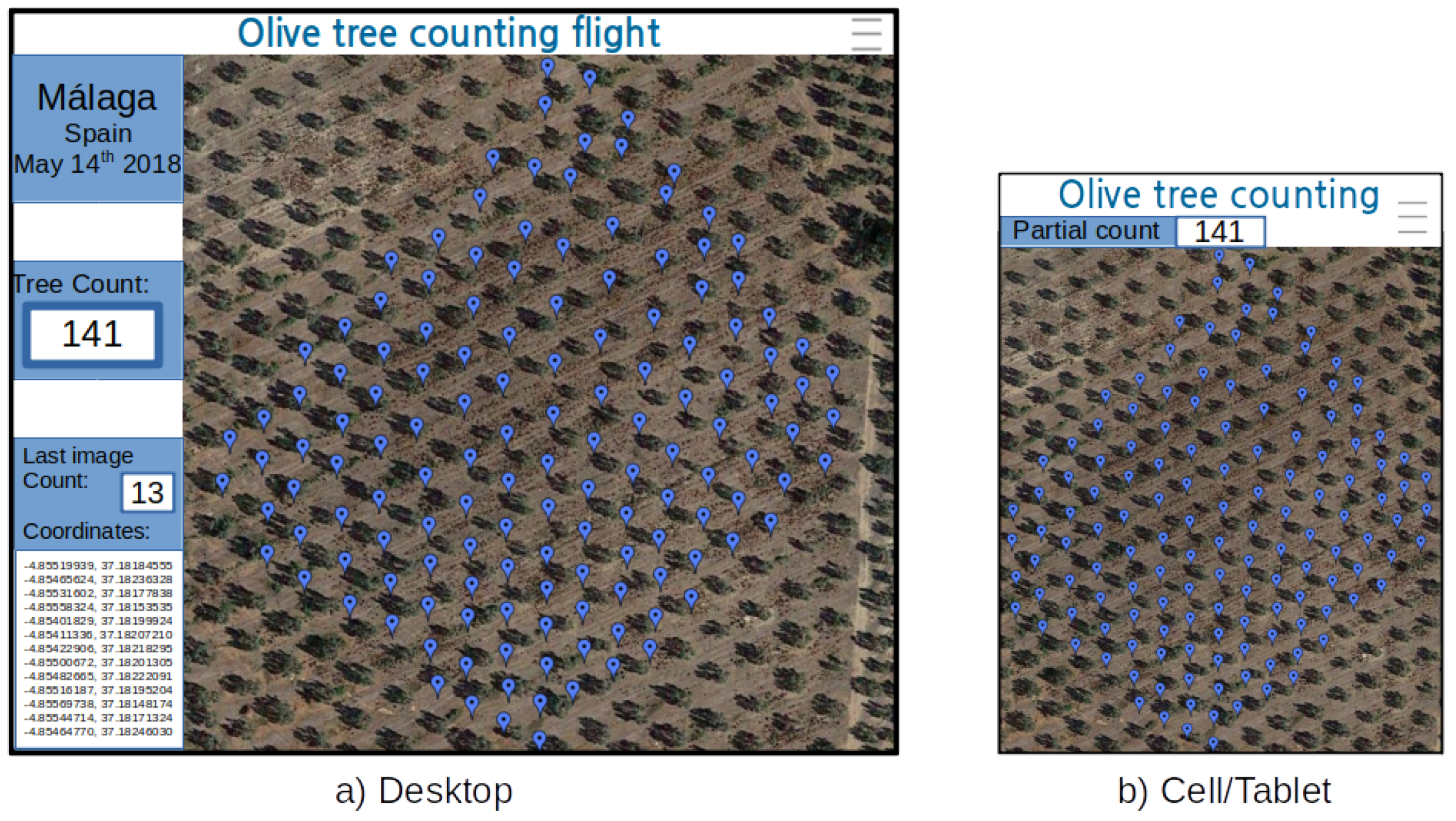
The UAV flight is managed by a service provider company in charge of a turnkey solution. The services include the preparation of the flight plan and the permits for flights, the actual flight, and the data delivery. For the data delivery, the company has a cloud service and a client application that connects to the data channel of the client. The client application has two versions: the desktop and the mobile device, with slightly different interfaces to best output to the screen of the device. However, both versions share the same kernel consisting of a light web browser. This web browser opens the fixed Internet address where the cloud server channel is connected. A screenshot of the two versions can be seen in Figure 12. The calculated geolocation of the trees cannot be further validated due to the lack of the ground-truth coordinates of any tree.
Before the flight, the application shows a map of the area with an overlay of the UAV flight plan and the estimated take-off time. Once the UAV takes off, the screen shows the partial count number of trees inventoried to the moment. Every two seconds, a new image is captured and processed, and the new detected trees are added to the counter. In the desktop application, the partial count of the new image is also shown, together with the geolocation of these last trees. As demonstrated in [42], the delay of the mqtt protocol is lower than using the httpprotocol, consumes less power, and is able to send a message to one thousand clients with only one operation.
On the map, the application sets a place mark on each location where a tree is detected. Clicking on the place mark provides information about the geolocation of the tree and about the pixel locations of all the images where this tree can be seen. Clicking on the row of the coordinates of a tree will have the same effects.
5. Conclusions
The value of an unmanned system is in its ability to carry out a specific job whose ultimate goal is to provide useful information to the end-user. Data processing and analysis can take a long time before obtaining the final product, which is then delivered to the end-user, usually in the form of maps or reports. In this work, we have shown that the processing capabilities of current embedded processors can be combined with existing cloud services for a fast delivery of the relevant information and using easy visualization tools found in current personal devices. As an example use case, we implemented an application to count the number of olive trees in a crop field during flight, using an incremental segmentation algorithm on each of the images as the data were being acquired. Processing includes segmentation of trees, individual geolocation, and image overlapping corrections. The partial information that is available (the trees’ geolocation) is published in the cloud, where end-users can obtain straightforward visualization. In less than 20 s, the application detected and counted 330 olive trees out of a total of 332 reference trees for a sequence of 10 images. The resulting accuracy was higher than 99%, improving the accuracy of similar works that processed one mosaic image using off-line software. Although color-based segmentation has provided very good results in this experiment, we will consider using machine learning algorithms for future works on tree recognition, especially for more noisy images, such as forests. Moreover, the use of simultaneous localization and mapping (SLAM) techniques can be a complementary solution to improve the geolocation accuracy. As pending work, we shall obtain the ground-truth trees’ coordinates to be able to validate the trees’ geolocation results. Many new UAS applications, not only in rural areas, but also in populated areas, will require the increase of the processing capabilities on board the UAV. The proposed architecture can be applicable to them when the outcome of the flight needs to be shared rapidly.
Author Contributions
Conceptualization, E.S., A.G., and C.B.; formal analysis, E.S. and C.B.; funding acquisition, C.B.; investigation, E.S., A.G., and C.B.; methodology, E.S.; resources, A.G.; software, E.S., A.G., and G.S.; supervision, C.B.; validation, E.S.; visualization, E.S. and C.B.; writing, E.S., G.S., and C.B.
Funding
This work was funded by the Ministry of Economy, Industry and Competitiveness of Spain under Grant Number TRA2016-77012-R.
Acknowledgments
We thank the reviewers for the valuable comments they provided.
Conflicts of Interest
The authors declare no conflict of interest.
References
- Saari, H.; Akujärvi, A.; Holmlund, C.; Ojanen, H.; Kaivosoja, J.; Nissinen, A.; Niemeläinen, O. Visible, Very Near IR and Short Wave IR Hyperspectral Drone Imaging System for Agriculture and Natural Water Applications. ISPRS Int. Arch. Photogramm. Remote Sens. Spat. Inf. Sci. 2017, 165–170. [Google Scholar] [CrossRef]
- Salamí, E.; Barrado, C.; Pastor, E. UAV Flight Experiments Applied to the Remote Sensing of Vegetated Areas. Remote Sens. 2014, 6, 11051–11081. [Google Scholar] [CrossRef]
- Ballester, M.; Victoria, D.C.; Krusche, A.; Coburn, R.; Victoria, R.; Richey, J.; Logsdon, M.; Mayorga, E.; Matricardi, E. A remote sensing/GIS-based physical template to understand the biogeochemistry of the Ji-Paraná river basin (Western Amazônia). Remote Sens. Environ. 2003, 87, 429–445. [Google Scholar] [CrossRef]
- Capolupo, A.; Kooistra, L.; Berendonk, C.; Boccia, L.; Suomalainen, J. Estimating Plant Traits of Grasslands from UAV-Acquired Hyperspectral Images: A Comparison of Statistical Approaches. ISPRS Int. J. Geo-Inf. 2015, 4, 2792–2820. [Google Scholar] [CrossRef]
- Pádua, L.; Vanko, J.; Hruška, J.; Adão, T.; Sousa, J.J.; Peres, E.; Morais, R. UAS, sensors, and data processing in agroforestry: A review towards practical applications. Int. J. Remote Sens. 2017, 38, 2349–2391. [Google Scholar] [CrossRef]
- Vu, Q.; Raković, M.; Delic, V.; Ronzhin, A. Trends in Development of UAV-UGV Cooperation Approaches in Precision Agriculture. In Proceedings of the International Conference on Interactive Collaborative Robotics, Leipzig, Germany, 18–22 September 2018; Springer: Berlin/Heidelberg, Germany, 2018; pp. 213–221. [Google Scholar]
- Pix4D. Pix4Dmapper. 2016. Available online: https://www.pix4d.com/product/pix4dmapper-photogrammetry-software (accessed on 13 September 2018).
- SimActive. Correlator3D. 2018. Available online: https://www.simactive.com/correlator3d-mapping-software-features.html (accessed on 13 September 2018).
- Agisoft. PhotoScan. 2016. Available online: https://www.agisoft.es/products/agisoft-photoscan/ (accessed on 13 September 2018).
- Russ, J.C. The Image Processing Handbook; CRC Press: Boca Raton, FL, USA, 2016. [Google Scholar]
- Song, H.; Yang, C.; Zhang, J.; Hoffmann, W.C.; He, D.; Thomasson, J.A. Comparison of mosaicking techniques for airborne images from consumer-grade cameras. J. Appl. Remote Sens. 2016, 10, 016030. [Google Scholar] [CrossRef]
- Ma, Y.; Wu, H.; Wang, L.; Huang, B.; Ranjan, R.; Zomaya, A.; Jie, W. Remote sensing big data computing: Challenges and opportunities. Future Gener. Comput. Syst. 2015, 51, 47–60. [Google Scholar] [CrossRef]
- Khanal, S.; Fulton, J.; Shearer, S. An overview of current and potential applications of thermal remote sensing in precision agriculture. Comput. Electron. Agric. 2017, 139, 22–32. [Google Scholar] [CrossRef]
- Ma, Y.; Wang, L.; Zomaya, A.Y.; Chen, D.; Ranjan, R. Task-Tree Based Large-Scale Mosaicking for Massive Remote Sensed Imageries with Dynamic DAG Scheduling. IEEE Trans. Parallel Distrib. Syst. 2014, 25, 2126–2137. [Google Scholar] [CrossRef]
- Fernández-Guisuraga, J.M.; Sanz-Ablanedo, E.; Suárez-Seoane, S.; Calvo, L. Using Unmanned Aerial Vehicles in Postfire Vegetation Survey Campaigns through Large and Heterogeneous Areas: Opportunities and Challenges. Sensors 2018, 18, 586. [Google Scholar] [CrossRef]
- Lee, J. ODROID-XU3: The Fastest Computer Made by Hardkernel So Far! ODROID Mag. 2014, 10, 22–23. [Google Scholar]
- Shilpashree, K.; Lokesha, H.; Shivkumar, H. Implementation of Image Processing on Raspberry Pi. Int. J. Adv. Res. Comput. Commun. Eng. 2015, 4, 199–202. [Google Scholar]
- De Castro, A.I.; Torres-Sánchez, J.; Peña, J.M.; Jiménez-Brenes, F.M.; Csillik, O.; López-Granados, F. An Automatic Random Forest-OBIA Algorithm for Early Weed Mapping between and within Crop Rows Using UAV Imagery. Remote Sens. 2018, 10, 285. [Google Scholar] [CrossRef]
- She, Y.; Ehsani, R.; Robbins, J.; Leiva, J.N.; Owen, J. Applications of Small UAV Systems for Tree and Nursery Inventory Management. In Proceedings of the International Conference on Precision Agriculture (ICPA 2014), Sacramento, CA, USA, 20–23 July 2014. [Google Scholar]
- Perrin, G.; Descombes, X.; Zerubia, J. A marked point process model for tree crown extraction in plantations. In Proceedings of the IEEE International Conference on Image Processing, Genova, Italy, 14 September 2005; Volume 1. [Google Scholar] [CrossRef]
- Chen, S.W.; Shivakumar, S.S.; Dcunha, S.; Das, J.; Okon, E.; Qu, C.; Taylor, C.J.; Kumar, V. Counting apples and oranges with deep learning: A data-driven approach. IEEE Robot. Autom. Lett. 2017, 2, 781–788. [Google Scholar] [CrossRef]
- Kalantar, B.; Idrees, M.O.; Mansor, S.; Halin, A.A. Smart Counting–Oil Palm tree inventory with UAV. Coord. Mag. 2017, 13, 17–22. [Google Scholar]
- Dalponte, M.; Ørka, H.O.; Ene, L.T.; Gobakken, T.; Næsset, E. Tree crown delineation and tree species classification in boreal forests using hyperspectral and ALS data. Remote Sens. Environ. 2014, 140, 306–317. [Google Scholar] [CrossRef]
- Lee, J.; Cai, X.; Lellmann, J.; Dalponte, M.; Malhi, Y.; Butt, N.; Morecroft, M.; Schönlieb, C.B.; Coomes, D.A. Individual tree species classification from airborne multisensor imagery using robust PCA. IEEE J. Sel. Top. Appl. Earth Obs. Remote Sens. 2016, 9, 2554–2567. [Google Scholar] [CrossRef]
- Vaughn, N.R.; Moskal, L.M.; Turnblom, E.C. Tree species detection accuracies using discrete point lidar and airborne waveform lidar. Remote Sens. 2012, 4, 377–403. [Google Scholar] [CrossRef]
- Koch, B.; Kattenborn, T.; Straub, C.; Vauhkonen, J. Segmentation of forest to tree objects. In Forestry Applications of Airborne Laser Scanning; Springer: Berlin/Heidelberg, Germany, 2014; pp. 89–112. [Google Scholar]
- Zarco-Tejada, P.J.; Diaz-Varela, R.; Angileri, V.; Loudjani, P. Tree height quantification using very high resolution imagery acquired from an unmanned aerial vehicle (UAV) and automatic 3D photo-reconstruction methods. Eur. J. Agron. 2014, 55, 89–99. [Google Scholar] [CrossRef]
- Bazi, Y.; Malek, S.; Alajlan, N.; AlHichri, H. An automatic approach for palm tree counting in UAV images. In Proceedings of the 2014 IEEE International Geoscience and Remote Sensing Symposium (IGARSS), Quebec City, QC, Canada, 13–18 July 2014; pp. 537–540. [Google Scholar]
- Nevalainen, O.; Honkavaara, E.; Tuominen, S.; Viljanen, N.; Hakala, T.; Yu, X.; Hyyppä, J.; Saari, H.; Pölönen, I.; Imai, N.N.; et al. Individual tree detection and classification with UAV-based photogrammetric point clouds and hyperspectral imaging. Remote Sens. 2017, 9, 185. [Google Scholar] [CrossRef]
- Fassnacht, F.E.; Latifi, H.; Stereńczak, K.; Modzelewska, A.; Lefsky, M.; Waser, L.T.; Straub, C.; Ghosh, A. Review of studies on tree species classification from remotely sensed data. Remote Sens. Environ. 2016, 186, 64–87. [Google Scholar] [CrossRef]
- Larsen, M.; Eriksson, M.; Descombes, X.; Perrin, G.; Brandtberg, T.; Gougeon, F.A. Comparison of six individual tree crown detection algorithms evaluated under varying forest conditions. Int. J. Remote Sens. 2011, 32, 5827–5852. [Google Scholar] [CrossRef]
- Kaartinen, H.; Hyyppä, J.; Yu, X.; Vastaranta, M.; Hyyppä, H.; Kukko, A.; Holopainen, M.; Heipke, C.; Hirschmugl, M.; Morsdorf, F.; et al. An international comparison of individual tree detection and extraction using airborne laser scanning. Remote Sens. 2012, 4, 950–974. [Google Scholar] [CrossRef]
- Kattenborn, T.; Sperlich, M.; Bataua, K.; Koch, B. Automatic single tree detection in plantations using UAV-based photogrammetric point clouds. Int. Arch. Photogramm. Remote Sens. Spat. Inf. Sci. 2014, 40, 139. [Google Scholar] [CrossRef]
- Dechesne, C.; Mallet, C.; Le Bris, A.; Gouet, V.; Hervieu, A. Forest stand segmentation using airbone LiDAR data and very high resolution multispectral imagery. Int. Arch. Photogramm. Remote Sens. Spat. Inf. Sci. 2016, 41, 207–214. [Google Scholar] [CrossRef]
- Onishi, M.; Ise, T. Automatic classification of trees using a UAV onboard camera and deep learning. arXiv, 2018; arXiv:1804.10390. [Google Scholar]
- Sandino, J.; Pegg, G.; Gonzalez, F.; Smith, G. Aerial Mapping of Forests Affected by Pathogens Using UAVs, Hyperspectral Sensors, and Artificial Intelligence. Sensors 2018, 18, 944. [Google Scholar] [CrossRef]
- Ryan, D.; Denman, S.; Sridharan, S.; Fookes, C. An evaluation of crowd counting methods, features and regression models. Comput. Vis. Image Underst. 2015, 130, 1–17. [Google Scholar] [CrossRef]
- Zhao, X.; Dellandrea, E.; Chen, L.; Kakadiaris, I.A. Accurate landmarking of three-dimensional facial data in the presence of facial expressions and occlusions using a three-dimensional statistical facial feature model. IEEE Trans. Syst. Man Cybern. Part B 2011, 41, 1417–1428. [Google Scholar] [CrossRef]
- Wateosot, C.; Suvonvorn, N. Top-view Based People Counting Using Mixture of Depth and Color Information. In Proceedings of the Second Asian Conference on Information Systems, Phuket, Thailand, 31 October–2 November 2013. [Google Scholar]
- Lee, C.A.; Gasster, S.D.; Plaza, A.; Chang, C.I.; Huang, B. Recent developments in high performance computing for remote sensing: A review. IEEE J. Sel. Top. Appl. Earth Obs. Remote Sens. 2011, 4, 508–527. [Google Scholar] [CrossRef]
- Wang, P.; Wang, J.; Chen, Y.; Ni, G. Rapid processing of remote sensing images based on cloud computing. Future Gener. Comput. Syst. 2013, 29, 1963–1968. [Google Scholar] [CrossRef]
- Abdelwahab, S.; Hamdaoui, B.; Guizani, M.; Rayes, A. Enabling smart cloud services through remote sensing: An internet of everything enabler. IEEE Internet Things J. 2014, 1, 276–288. [Google Scholar] [CrossRef]
- Jain, S.; Fall, K.; Patra, R. Routing in a Delay Tolerant Network. SIGCOMM Comput. Commun. Rev. 2004, 34, 145–158. [Google Scholar] [CrossRef]
- García-Mateos, G.; Hernández-Hernández, J.; Escarabajal-Henarejos, D.; Jaen-Terrones, S.; Molina-Martínez, J. Study and comparison of color models for automatic image analysis in irrigation management applications. Agric. Water Manag. 2015, 151, 158–166. [Google Scholar] [CrossRef]
- Otsu, N. A Threshold Selection Method from Gray-Level Histograms. IEEE Trans. Syst. Man Cybern. 1979, 9, 62–66. [Google Scholar] [CrossRef]
- Konolige, K. Small Vision Systems: Hardware and Implementation. In Proceedings of the 8th International Symposium in Robotic Research, Hayama, Japan, 3–7 October 1997; pp. 203–212. [Google Scholar]
- Bay, H.; Tuytelaars, T.; Gool, L.V. Surf: Speeded up robust features. In European Conference on Computer Vision; Springer: Berlin/Heidelberg, Germany, 2006; pp. 404–417. [Google Scholar]
- Hirschmuller, H. Stereo processing by semiglobal matching and mutual information. IEEE Trans. Pattern Anal. Mach. Intell. 2008, 30, 328–341. [Google Scholar] [CrossRef] [PubMed]
- Jain, A. Fundamentals of Digital Image Processing; Prentice-Hall: Uapper Saddle River, NJ, USA, 1986. [Google Scholar]
- Suzuki, S.; Abe, K. Topological Structural Analysis of Digitized Binary Images by Border Following. CVGIP 1985, 30, 32–46. [Google Scholar]
- Mount, D.M.; Arya, S. ANN: A Library for Approximate Nearest Neighbor Searching. 2010. Available online: http://www.cs.umd.edu/~mount/ANN/ (accessed on 30 May 2018).
- Salamí, E.; Barrado, C.; Pérez-Batlle, M.; Royo, P.; Santamaria, E.; Pastor, E. Fast Geolocation for Hot Spot Detection. In Proceedings of the 34th International Conference on Remote Sensing of Environment, Sydney, Australia, 10–15 April 2011. [Google Scholar]
- Qiu, T.; Zhao, A.; Ma, R.; Chang, V.; Liu, F.; Fu, Z. A task-efficient sink node based on embedded multi-core soC for Internet of Things. Future Gener. Comput. Syst. 2016, 82, 656–666. [Google Scholar] [CrossRef]
- Krishna, P.G.; Ravi, K.S.; Kumar, V.S.; Kumar, M.S. Implementation of mqtt protocol on low resourced embedded netork. Int. J. Pure Appl. Math. IJPAM 2017, 116, 161–166. [Google Scholar]
- Jara, A.J.; Bocchi, Y.; Fernandez, D.; Molina, G.; Gomez, A. An analysis of context-aware data models for smart cities: Towards fiware and etsi cim emerging data model. Int. Arch. Photogramm. Remote Sens. Spat. Inf. Sci. 2017, 42, 43. [Google Scholar] [CrossRef]
- Lerner, R.M. At the Forge Syndication with RSS. Linux J. 2004, 2004, 1–6. [Google Scholar]
- Godil, A.; Bostelman, R.; Shackleford, W.; Hong, T.; Shneier, M. Performance Metrics for Evaluating Object and Human Detection and Tracking Systems; Technical Report; NIST Interagency/Internal Report (NISTIR)-7972; National Institute of Standards and Technology: Gaithersburg, MD, USA, 2014.
- Mohan, M.; Silva, C.A.; Klauberg, C.; Jat, P.; Catts, G.; Cardil, A.; Hudak, A.T.; Dia, M. Individual tree detection from unmanned aerial vehicle (UAV) derived canopy height model in an open canopy mixed conifer forest. Forests 2017, 8, 340. [Google Scholar] [CrossRef]
Figure 1.
Aerial view of the area.

Figure 2.
Original UAV used to capture the images and tested embedded board. (a) DJI Phantom4. (b) RaspberryPi.
Figure 2.
Original UAV used to capture the images and tested embedded board. (a) DJI Phantom4. (b) RaspberryPi.

Figure 3.
Tree counting data processing flow (L1 is a list with the pixel coordinates of the trees detected in one image; L2 is the same list with pixel coordinates projected to a global reference system; and L3 is a global list with the coordinates of the trees detected in all the processed images without duplicates).

Figure 4.
Flowchart of the color-based segmentation algorithm (x, y, and r are are the center pixel coordinates and the radius of the circle enclosing the detected trees; L1 is the output list with the image pixel coordinates of the detected trees).
Figure 4.
Flowchart of the color-based segmentation algorithm (x, y, and r are are the center pixel coordinates and the radius of the circle enclosing the detected trees; L1 is the output list with the image pixel coordinates of the detected trees).

Figure 5.
Images corresponding to the intermediate steps when applying the color-based segmentation algorithm to the image DJI_0225. (a) Color-based thresholding. (b) Distance transform and template (top left). (c) Template matching. (d) Detected trees.
Figure 5.
Images corresponding to the intermediate steps when applying the color-based segmentation algorithm to the image DJI_0225. (a) Color-based thresholding. (b) Distance transform and template (top left). (c) Template matching. (d) Detected trees.

Figure 6.
Images corresponding to the intermediate steps when applying the stereo vision-based segmentation algorithm to the image DJI_0225. (a) Rectified images using epipolar geometry (epipolar lines are shown in green). (b) Adaptive threshold on the disparity matrix. (c) Detected trees.
Figure 6.
Images corresponding to the intermediate steps when applying the stereo vision-based segmentation algorithm to the image DJI_0225. (a) Rectified images using epipolar geometry (epipolar lines are shown in green). (b) Adaptive threshold on the disparity matrix. (c) Detected trees.

Figure 7.
Flowcharts of the registration and merge algorithms (L1 is the list with the pixel coordinates of the trees detected in the image; L2 is the same list with pixel coordinates projected to a global reference system; and L3 is the list with the coordinates of the trees detected in all the processed images without duplicates). (a) Registration. (b) Merge.

Figure 8.
The architecture of the drone-in-the-cloud solution is able to deliver the relevant information to the end-users on their own devices during the UAV flight.
Figure 8.
The architecture of the drone-in-the-cloud solution is able to deliver the relevant information to the end-users on their own devices during the UAV flight.

Figure 9.
Different associations when matching ground-truth (yellow crosses) and detected trees (white circles). (a) One-to-one (TP = 1). (b) One-to-zero (FN = 1). (c) Zero-to-one (FP = 1). (d) Many-to-one (TP = 1, FN = 1).
Figure 9.
Different associations when matching ground-truth (yellow crosses) and detected trees (white circles). (a) One-to-one (TP = 1). (b) One-to-zero (FN = 1). (c) Zero-to-one (FP = 1). (d) Many-to-one (TP = 1, FN = 1).

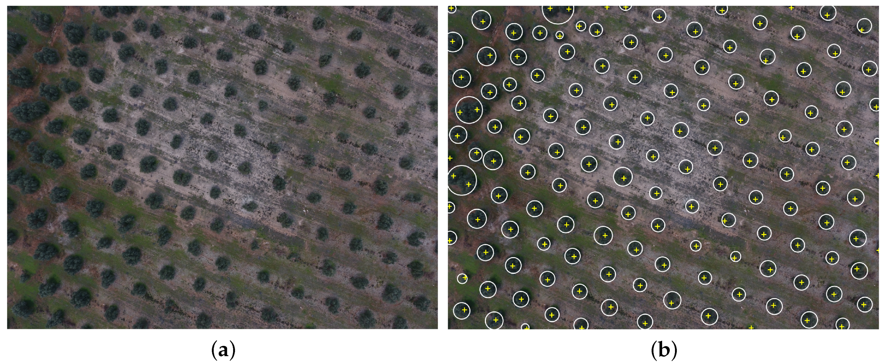
Figure 10.
Color-based segmentation results (white circles) vs. ground-truth reference (yellow crosses) for image DJI_0232 (worst case). (a) Original image. (b) Detected and annotated trees.
Figure 10.
Color-based segmentation results (white circles) vs. ground-truth reference (yellow crosses) for image DJI_0232 (worst case). (a) Original image. (b) Detected and annotated trees.

Figure 11.
Tree detection in a sequence of 10 images.

Figure 12.
User application interface on different devices.


Table 1.
Comparison of the number of olive trees counted by the color-based and the stereo vision-based segmentation algorithms. Results are compared with respect to the number of hand-annotated olive trees (GT: ground-truth, AE: absolute error, MAE: mean absolute error, RMSE: root mean squared error).
| Color-Based | Stereo Vision-Based | ||||||
|---|---|---|---|---|---|---|---|
| Image | GT | Count | AE | Image | GT | Count | AE |
| DJI_0225 | 107 | 106 | 1 | DJI_0225-DJI_0226 | 75 | 52 | 23 |
| DJI_0226 | 115 | 114 | 1 | DJI_0226-DJI_0227 | 79 | 56 | 23 |
| DJI_0227 | 117 | 115 | 2 | DJI_0227-DJI_0228 | 82 | 50 | 32 |
| DJI_0228 | 115 | 115 | 0 | DJI_0228-DJI_0229 | 82 | 58 | 24 |
| DJI_0229 | 119 | 117 | 2 | DJI_0229-DJI_0230 | 84 | 56 | 28 |
| DJI_0230 | 125 | 120 | 5 | DJI_0230-DJI_0231 | 86 | 57 | 29 |
| DJI_0231 | 130 | 125 | 5 | DJI_0231-DJI_0232 | 89 | 56 | 33 |
| DJI_0232 | 139 | 130 | 9 | DJI_0232-DJI_0233 | 95 | 60 | 35 |
| DJI_0233 | 141 | 138 | 3 | DJI_0233-DJI_0234 | 101 | 53 | 48 |
| DJI_0234 | 143 | 142 | 1 | DJI_0234-DJI_0235 | 97 | 57 | 40 |
| MAE: | 2.90 | MAE: | 31.50 | ||||
| RMSE: | 3.89 | RMSE: | 32.41 | ||||
Table 2.
Classification performance metrics for each image (GT: ground-truth, TP: true positive, FP: false positive, FN: false negative, (-b): excluding errors in the borderline).
Table 2.
Classification performance metrics for each image (GT: ground-truth, TP: true positive, FP: false positive, FN: false negative, (-b): excluding errors in the borderline).
| Image | GT | Count | TP | FP | FN (-b) | Precision | Recall (-b) | Score (-b) |
|---|---|---|---|---|---|---|---|---|
| DJI_0225 | 107 | 106 | 107 | 0 | 1 (0) | 100.00 | 99.07 (100.00) | 99.53 (100.00) |
| DJI_0226 | 115 | 114 | 114 | 0 | 1 (0) | 100.00 | 99.13 (100.00) | 99.56 (100.00) |
| DJI_0227 | 117 | 115 | 115 | 0 | 2 (0) | 100.00 | 98.29 (100.00) | 99.14 (100.00) |
| DJI_0228 | 115 | 115 | 114 | 1 | 1 (0) | 99.13 | 99.13 (100.00) | 99.13 (99.56) |
| DJI_0229 | 119 | 117 | 117 | 0 | 2 (1) | 100.00 | 98.32 (99.15) | 99.15 (99.57) |
| DJI_0230 | 125 | 120 | 120 | 0 | 5 (1) | 100.00 | 96.00 (99.17) | 97.96 (99.59) |
| DJI_0231 | 130 | 125 | 125 | 0 | 5 (2) | 100.00 | 96.15 (98.43) | 98.04 (99.21) |
| DJI_0232 | 139 | 130 | 130 | 0 | 9 (3) | 100.00 | 93.53 (97.74) | 96.65 (98.86) |
| DJI_0233 | 141 | 138 | 137 | 1 | 4 (2) | 99.28 | 97.16 (98.56) | 98.21 (98.92) |
| DJI_0234 | 143 | 142 | 142 | 0 | 1 (1) | 100.00 | 99.30 (99.30) | 99.65 (99.65) |
| Average | 125 | 122 | 122 | 0.2 | 3.1 (1) | 99.84 | 97.61 (99.24) | 98.70 (99.54) |
Table 3.
Classification performance metrics with different template sizes (d, s) for image DJI_0232 (d: diameter, s: side size, GT: ground-truth, TP: true positive, FP: false positive, FN: false negative, (-b): excluding errors in the borderline).
Table 3.
Classification performance metrics with different template sizes (d, s) for image DJI_0232 (d: diameter, s: side size, GT: ground-truth, TP: true positive, FP: false positive, FN: false negative, (-b): excluding errors in the borderline).
| Template | GT | Count | TP | FP | FN (-b) | Precision | Recall (-b) | Score (-b) | |
|---|---|---|---|---|---|---|---|---|---|
| d = 20 | s = 40 | 139 | 163 | 133 | 30 | 6 (3) | 81.60 | 95.68 (97.79) | 88.08 (88.96) |
| s = 60 | 139 | 141 | 133 | 8 | 6 (3) | 94.33 | 95.68 (97.79) | 95.00 (96.03) | |
| s = 80 | 139 | 134 | 132 | 2 | 7 (3) | 98.51 | 94.96 (97.78) | 96.70 (98.14) | |
| d = 30 | s = 60 | 139 | 139 | 133 | 6 | 6 (3) | 95.68 | 95.68 (97.79) | 95.68 (96.73) |
| s = 80 | 139 | 130 | 130 | 0 | 9 (3) | 100.00 | 93.53 (97.74) | 96.65 (98.86) | |
| s = 100 | 139 | 128 | 128 | 0 | 11 (3) | 100.00 | 92.09 (97.71) | 95.88 (98.84) | |
| d = 40 | s = 80 | 139 | 128 | 128 | 0 | 11 (5) | 100.00 | 92.09 (96.24) | 95.88 (98.08) |
| s = 100 | 139 | 126 | 126 | 0 | 13 (5) | 100.00 | 90.65 (96.18) | 95.09 (98.05) | |
| s = 120 | 139 | 124 | 124 | 0 | 15 (6) | 100.00 | 89.21 (95.38) | 94.30 (97.64) | |
Table 4.
Classification performance metrics for a sequence of 10 images (GT: ground-truth, TP: true positive, FP: false positive, FN: false negative, (-b): excluding errors in the borderline).
Table 4.
Classification performance metrics for a sequence of 10 images (GT: ground-truth, TP: true positive, FP: false positive, FN: false negative, (-b): excluding errors in the borderline).
| Images | GT | Count | TP | FP | FN (-b) | Precision | Recall (-b) | Score (-b) |
|---|---|---|---|---|---|---|---|---|
| DJI_0225-DJI_0234 | 332 | 330 | 328 | 2 | 4 (3) | 99.39 | 98.80 (99.09) | 99.09 (99.24) |
Table 5.
Execution time of the proposed algorithms on the RaspberryPi 3. Mean and standard deviation per image. Time is in seconds.
Table 5.
Execution time of the proposed algorithms on the RaspberryPi 3. Mean and standard deviation per image. Time is in seconds.
| Algorithm | Mean (s) | StdDev (s) |
|---|---|---|
| Color-based segmentation | 0.5840 | 0.0148 |
| Stereo vision-based segmentation | 205.2 | 27.1 |
| Registration and merging | 0.4505 | 0.0120 |
| Geolocation | 0.0010 | 0.0002 |
© 2019 by the authors. Licensee MDPI, Basel, Switzerland. This article is an open access article distributed under the terms and conditions of the Creative Commons Attribution (CC BY) license (http://creativecommons.org/licenses/by/4.0/).
Share and Cite
MDPI and ACS Style
Salamí, E.; Gallardo, A.; Skorobogatov, G.; Barrado, C. On-the-Fly Olive Tree Counting Using a UAS and Cloud Services. Remote Sens. 2019, 11, 316. https://doi.org/10.3390/rs11030316
AMA Style
Salamí E, Gallardo A, Skorobogatov G, Barrado C. On-the-Fly Olive Tree Counting Using a UAS and Cloud Services. Remote Sensing. 2019; 11(3):316. https://doi.org/10.3390/rs11030316
Chicago/Turabian StyleSalamí, Esther, Antonia Gallardo, Georgy Skorobogatov, and Cristina Barrado. 2019. "On-the-Fly Olive Tree Counting Using a UAS and Cloud Services" Remote Sensing 11, no. 3: 316. https://doi.org/10.3390/rs11030316
Note that from the first issue of 2016, this journal uses article numbers instead of page numbers. See further details here.