Predicting Taxi Demand Based on 3D Convolutional Neural Network and Multi-task Learning


1
School of Computer Science and Engineering, Central South University, Changsha 410075, China
2
School of Computer and Information Engineering, Shanghai Polytechnic University, Shanghai 201209, China
*
Author to whom correspondence should be addressed.
Remote Sens. 2019, 11(11), 1265; https://doi.org/10.3390/rs11111265
Submission received: 20 April 2019
/
Revised: 22 May 2019
/
Accepted: 25 May 2019
/
Published: 28 May 2019
(This article belongs to the Special Issue Advanced Communication and Networking Techniques for Remote Sensing)
Abstract
:Taxi demand can be divided into pick-up demand and drop-off demand, which are firmly related to human’s travel habits. Accurately predicting taxi demand is of great significance to passengers, drivers, ride-hailing platforms and urban managers. Most of the existing studies only forecast the taxi demand for pick-up and separate the interaction between spatial correlation and temporal correlation. In this paper, we first analyze the historical data and select three highly relevant parts for each time interval, namely closeness, period and trend. We then construct a multi-task learning component and extract the common spatiotemporal feature by treating the taxi pick-up prediction task and drop-off prediction task as two related tasks. With the aim of fusing spatiotemporal features of historical data, we conduct feature embedding by attention-based long short-term memory (LSTM) and capture the correlation between taxi pick-up and drop-off with 3D ResNet. Finally, we combine external factors to simultaneously predict the taxi demand for pick-up and drop-off in the next time interval. Experiments conducted on real datasets in Chengdu present the effectiveness of the proposed method and show better performance in comparison with state-of-the-art models.

1. Introduction
The transportation system is to the city as the blood tissue is to the human body, and it is the key to urban construction. In the future, it will play an essential role in the construction of smart cities. With the development of Didi Chuxing and Uber, online car-hailing has become a travel habit of people. Therefore, extensive data on taxi demand have been collected for research. Accurate taxi demand forecast can help passengers avoid hot spots reasonably and save waiting time. It also can help drivers choose hot spots rationally and make a better balance between benefits and efficiency. For the online car-hailing platform, they can plan better and pre-allocate resources to maximize the benefits. For city managers, it can provide reference suggestions for infrastructure construction and traffic planning. Therefore, how to accurately predict future taxi demand in various regions of the city based on historical data has become a hot area of research.
In literature, traffic data prediction problem has been widely studied in the past, including traffic volume, taxi demand and travel time. Time series prediction methods and machine learning methods are first applied to traffic data prediction; representative algorithms include autoregressive integrated moving average (ARIMA) and its variants [1,2,3], and support vector machine (SVM) and its variants, respectively. However, such methods ignore the spatial correlation of data. In recent years, deep learning, which has achieved great success in computer vision and natural language process [4], has been widely used to traffic prediction [5]. Convolution neural network (CNN) and recurrent neural network (RNN) are used to catch temporal correlation [6,7,8] and spatial correlation [9,10], respectively. Models combining CNN, RNN and their variants are also widely used in traffic data prediction [11,12,13]; such methods usually use CNN to extract spatial features first, then use RNN to extract temporal features and finally make predictions.
However, accurate traffic data prediction still faces three significant challenges:
- First of all, traffic data are affected by complex spatial–temporal correlation, and there is an apparent periodicity in traffic data. Traffic states between different regions will affect each other, and there may be interactions between regions that are far away. Although the models combining CNN, RNN and their variants have achieved good results, this kind of method separates the interaction between temporal correlation and spatial correlation.
- Secondly, there is little work in predicting taxi drop-off demand. If there is a high taxi demand for drop-off in a particular region at a certain time, the vacancy rate of taxis in this region will be high, and it will be required for reasonable evacuation. At the same time, the high traffic volume will be a test for the infrastructure and road conditions of the corresponding region. Therefore, predicting taxi demand for drop-off can provide advice to taxi drivers and city managers. Besides, taxi demand for pick-up and drop-off may affect each other, since empty cars may stimulate people’s desire to take a taxi and increase the number of taxi pick-ups in surrounding areas.
To tackle the above challenges, this paper proposes a method to predict taxi demand for pick-up and drop-off in various regions of the city based on multi-task learning (MTL) and 3D convolutional neural networks (3D CNN). In detail, to begin, we first selected highly relevant historical data at each time interval. Then we treated taxi pick-up demand prediction and taxi drop-off demand prediction as related tasks. We harnessed the power of MTL and 3D CNN to extract spatiotemporal features without separating the interaction between temporal correlation and spatial correlation. Secondly, for the purpose of fusing the extracted features of historical data, we embedded those feature representations into a tensor by attention-based long short-term memory (LSTM). Next, we regarded the tensor as a video consisting of frames that represented the demand status within half an hour, and we used 3D ResNet to capture the spatiotemporal correlation and the complex correlation between the taxi demand for pick-up and drop-off. Finally, we combined external factors to predict taxi demand for pick-up and drop-off at the same time. We conducted extensive experiments on a real-world dataset. Our contributions are summarized as follows:
- We propose to consider the prediction of taxi demand for pick-up and drop-off as related tasks, and we constructed a feature extraction component based on multi-task learning and 3D CNN to extract spatiotemporal features concurrently.
- We propose to deem the demand situation of the urban taxi as a video and use 3D CNN to capture the spatiotemporal correlation and the complex correlation between taxi demand for pick-up and drop-off.
- We combined external factors, such as weather, day of the week and public transport conditions, to simultaneously predict taxi demand for pick-up and drop-off.
- We conducted extensive theoretical analysis and experiments on a real-world dataset in Chengdu and achieved better performance and efficiency than other baselines.
The rest of the paper is organized as follows: Section 2 describes the related work of the traffic data prediction problem. Section 3 provides the problem definition. The method for predicting taxi demand for pick-up and drop-off is outlined in Section 4. Section 5 gives the experimental verification designs and results. Section 6 summarizes the whole paper.
2. Related Work
Machine learning has been widely used in various fields, such as recommendation system [14,15], service computing [16,17,18,19,20,21], prediction problem [22,23,24,25], edge computing [26,27], and so on. In recent years, deep learning has been widely used in many research fields with great success in the fields of computer vision and natural language processing [28,29,30]. Taking the speech recognition field as an example, according to Padmanabhan et al. [31], Hidden Markov Model (HMM), Gaussian Mixture Models (GMM), SVM, and Artificial neural network (ANN) have been applied in this field and achieved limited performance. Deep learning is also widely used in speech recognition [32,33], and by contrast, allows end-to-end learning and achieves better performance.
In addition, many areas use multi-task learning to improve the performance of the applications. Zhang et al. [34] proposed to classify multi-task supervised learning as two categories according to what to share. One is the feature-based MTL, where different tasks share a feature representation, and the other is the parameter-based MTL, where model parameters relate to different tasks. The former is further categorized into the feature transformation approach, the feature selection approach, and the deep-learning approach according to the approach of sharing features.
The traffic data prediction problem, comprised of traffic volume, traffic speed, travel time and taxi demand (our problem), has attracted the attention of many researchers; these approaches can be divided into two groups: traditional approaches and deep learning approaches.
2.1. Traditional Approach
Time series algorithms are first introduced into predicting traffic data in an ARIMA-like model. Hamed et al. [35] developed an ARIMA model to predict the traffic volume on urban arterials. From here on, to improve prediction performance, researchers applied many variants of ARIMA for traffic prediction [36,37].
On the other hand, machine learning algorithms are also widely used in this filed. Wu et al. [38] applied support vector regression for travel-time prediction, Zheng et al. [39] used a Bayesian model combined neural network for short-term freeway traffic flow prediction. Kuang et al. [40] proposed a two-level model, which combines a cost-sensitive Bayesian network and a weighted K-nearest neighbor model to predict the duration of traffic accidents. k-NN models are also widely applied in predicting traffic speeds and volume due to its simple nature [41,42].
These methods focus on the temporal correlation of traffic data, while neglecting its spatial correlation. However, the traffic conditions in the current region are affected not only by the adjacent region but also by regions farther away. For example, a traffic incident occurring in the intersection may render roads impassable, resulting in a dramatic increase in traffic volume at a remote transportation hub.
2.2. Deep Learning Approach
In recent years, deep learning methods have been widely used by many researchers in predicting traffic data. CNN has proved effective on extracting features from images. Thus, by treating the traffic condition of the entire city as an image, many researchers naturally started to employ CNN in traffic data prediction. Ma et al. [6] divided the city into many tiny grids, converting city traffic speed into images and use CNN for predicting traffic speed. Zhang et al. [7] employed CNN modeling temporal dependent (temporal closeness, period and seasonal trend) and spatial dependent for predicting traffic flow, rent/return of bikes and traffic flow. Later, Zhang et al. [8] used a residual neural network, a parametric-matrix-based fusion mechanism, and external information to improve the performance in predicting crowd flows. These studies focus more on the spatial correlation of traffic data. On the contrary, for modeling temporal correlation, they simply fusion features extracted by CNN through neural networks, which does not utilize temporal correlation sufficiently.
On the other hand, the success of RNN and its variants, that is, long short-term memory (LSTM) and gated recurrent units (GRU), in sequential learning tasks [43] has led many researchers to predict traffic data based on them. Zhao et al. [9] proposed using cascaded LSTM, where lateral dimension indicates the changes in the time domain and the vertical dimension indicates different observation points’ indexes, combined with an origin–destination correlation matrix to capture spatial–temporal correlation for predicting traffic flow. Xu et al. [10] applied LSTM and mixture density network to predict taxi demand in the city of New York. The model first predicts the entire probability distribution of taxi demands, then uses this probability distribution to decide taxi demand for each area. These studies focus more on capturing temporal correlation. However, they do not use spatial correlation sufficiently.
With the purpose of making full use of spatiotemporal correlation, many researchers combined CNN and RNN for predicting traffic data. Wu et al. [11] treated roads as a vector, which fed into 1D CNN to capture spatial correlation of traffic flow, and then used two LSTM to mine the short-term variability and periodicities of traffic flow. Yu et al. [12] proposed to apply deep CNN to extract spatial features which then fed to stacked LSTM for predicting large-scale transportation network traffic. Yao et al. [13] believed that applying CNN to the image of the entire city hurts prediction accuracy; for this reason, they utilized local CNN to capture spatial correlation and introduced a semantic view combined with LSTM to predict taxi demand. Although spatiotemporal correlation is taken into consideration in both instances, these studies separate the interaction between temporal correlation and spatial correlation.
In summary, previous studies separate the interaction between temporal correlation and spatial correlation, few studies predict taxi drop-off demand, and none of these studies take the interaction between taxi pick-up and taxi drop-off into consideration.
3. Preliminary
Definition 1 (Trip).
We defined a trip as a tuple (id,tpick,locationpick,tdrop,locationdrop), whereis the trip identification number,is the pick-up time,represents the pick-up location, tdrop is the drop-off time, locationdrop represents the drop-off location.
Definition 2 (Region Partition).
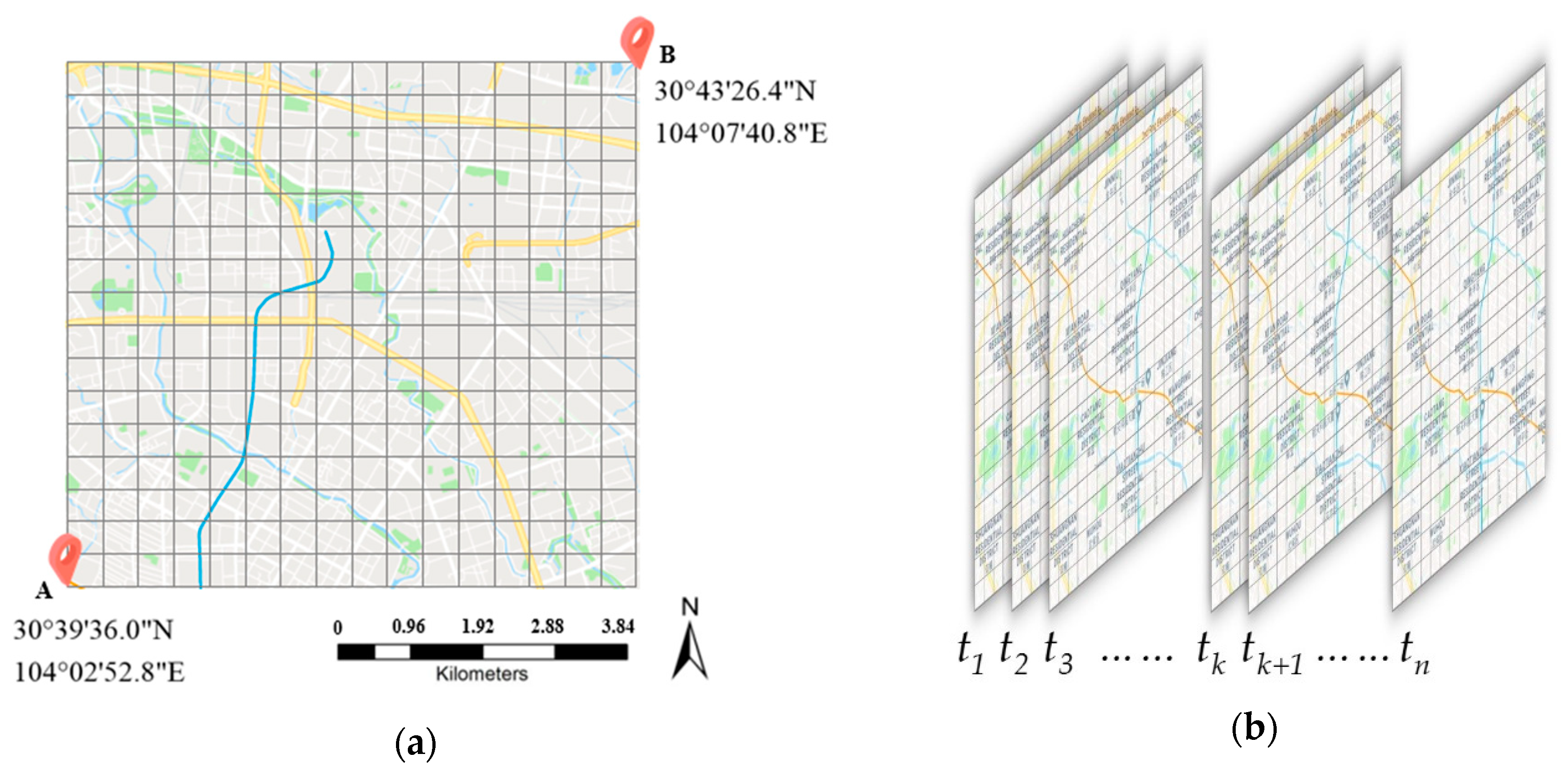
In the spatial view, we followed previous studies [44]. As shown in Figure 1a, let point A be the lowest left corner of the rectangle represented by the coordinates, and let point B be the top right corner of the rectangle represented by the coordinates. We partitioned the whole city intoequal grids. We usedandto represent the length of latitude and longitude of a grid, respectively. Where
we represented gridwhich lies as therow and thecolumn as
whereand.
Definition 3 (Pick-up/Drop-off Demand).
Following previous studies [8,44], for a certain, the taxi pick-up and taxi drop-off demand at the time intervalwere defined respectively as
At the time interval, demands in all regions were denoted as a tensorwhereand.
Problem 1:
Given , , and the historical demand tensors , predict .
4. Method
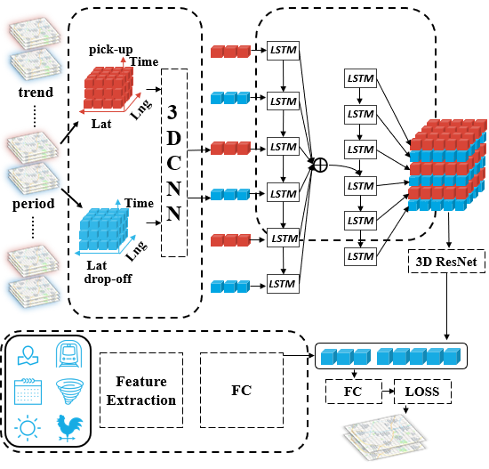
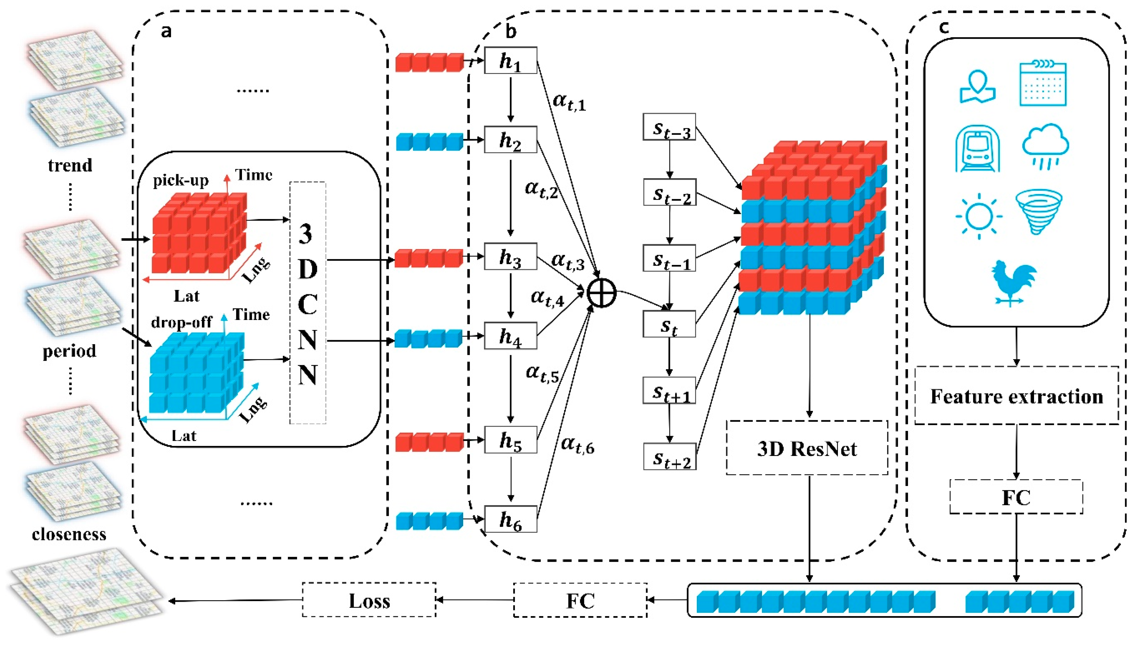
Figure 2 presents the framework of our proposed model Taxi3D. We first selected parts of historical data, which are highly relevant to the future demand situation. Secondly, we extracted common spatiotemporal features by MTL-based 3D CNN from two related tasks, that is, a taxi pick-up prediction task and a taxi drop-off prediction task. Later, we used attention-based LSTM embedding spatiotemporal features into a tensor which fed into the 3D ResNet and transformed into a vector. Meanwhile, external information, such as meteorological features, was also encoded into vectors. Finally, we concatenated the above two vectors and simultaneously predicted taxi demand for pick-up and drop-off in the next interval.
Accordingly, our model is composed of four major components, which as follows: (1) Multi-task spatiotemporal feature extraction component, in which we capture spatiotemporal correlations. (2) Feature embedding component. In this module, we fused spatiotemporal features into a tensor, then captured correlations between taxi pick-up and taxi drop-off and obtained the representation vector . (3) External factors component, where external information (e.g., weather condition, holidays, etc.) were encoded into representation . (4) Prediction component. We combined and to predict future demand.
In this section, we detailed our proposed method by a running example. The historical demand data inputted into our model are defined as a four-dimensional tensor:
- is the category of data, that is, for taxi pick-up data and taxi drop-off data.
- is the depth of data.
- is the number of grid columns.
- is the number of grid rows.
For example, at time interval , we may concatenate as the input tensor of the model.
4.1. Partition of Historical Data
As shown in Figure 3, the demand in different areas presents a repetitive pattern; for example, the demand pattern of Friday in Figure 3c is similar to that of Thursday and last Friday. With spatiotemporal domain knowledge, we can effectively select this higher-dependent timestamps to reduce input size. To the best of our knowledge, a time series always has one, or two, or all of the following temporal properties: (1) Temporal closeness; (2) period; (3) trend [7]. In view of the fact that taxi demand not only exhibits an evident periodicity but is also affected by an adjacent time interval, we separately divided previous taxi pick-up data and taxi drop-off data into three parts: closeness, period and trend, which represents the near past, the same time yesterday and the same time last week respectively.
For example, at each time interval , we split input tensor into 6 parts: , , , , and , where , and represents closeness, period and trend respectively, and .
4.2. Multi-Task Spatiotemporal Feature Extraction Component
Figure 3 shows the number of taxi demands in three distinct regions in Chengdu from 5 November 2016, to 18 November 2016. Analyzing this data indicates that taxi pick-up demands and taxi drop-off demands were basically positively correlation; that is, when the demand for taxi pick-up was high, the demand for drop-off was also high, and vice versa. To capture such regularities, we conducted MLT in extracting features from historical data. In short, by sharing representations between related tasks, MTL can enable our model to learn several tasks at the same time with better generalization performance.
To be specific, in this study, two related tasks, taxi pick-up demand prediction and taxi drop-off demand prediction, were trained together. Different from previous studies, at each time interval , we firstly extracted features from taxi pick-up data and then used the same network extracts features from taxi drop-off data . Therefore, we got shared information in the feature extraction stage.
Furthermore, taxi demand in adjacent areas will also affect each other. Hence, the problem of predicting future taxi demand based on historical demand has some common ground with the problem of video generation, in which every frame and some pixels will affect each other. Motivated by the success of 3D CNN in human action recognition [45] and video analysis [46], we conducted feature extraction by 3D CNN.
The hidden layers of a CNN typically contain a series of convolutional layers and pooling layers. LeCun et al. [4] argue that the role of the convolutional layer is to extract features from data at different levels. With the interactions between layers, high-level features are obtained in the higher layers by composing low-level ones extracted in the lower layers. Yosinski et al. [47] visualized an eight-layer CNN, and the results showed that the lower layers could detect edges, corners, etc., while the higher layers could detect faces, handles, bottles, etc. As for the pooling layer, its function is to reduce spatial dimensions of the feature map, reducing the amount of parameters and computation, and thus control overfitting.
In our study, we constructed a K-layers 3D CNN to obtain complex spatiotemporal features. Among them, in the first K-1 layers, we used zero-padding to input tensor in the convolution operation. Zero-padding, on the one hand, ensures that the edges of the tensor are covered many times in the convolution operation, and on the other hand keeps the size of the feature map unchanged in convolution operation to fully capture the interaction between each area in the whole city. Besides, two areas in a city far away from each other may be connected by metro, thus making the demand patterns of the two places relevant. Therefore, we introduced dilated convolution and increased the stride size of convolution in the last layer, which not only reduces the size of the feature map, but also captures the remote dependence.
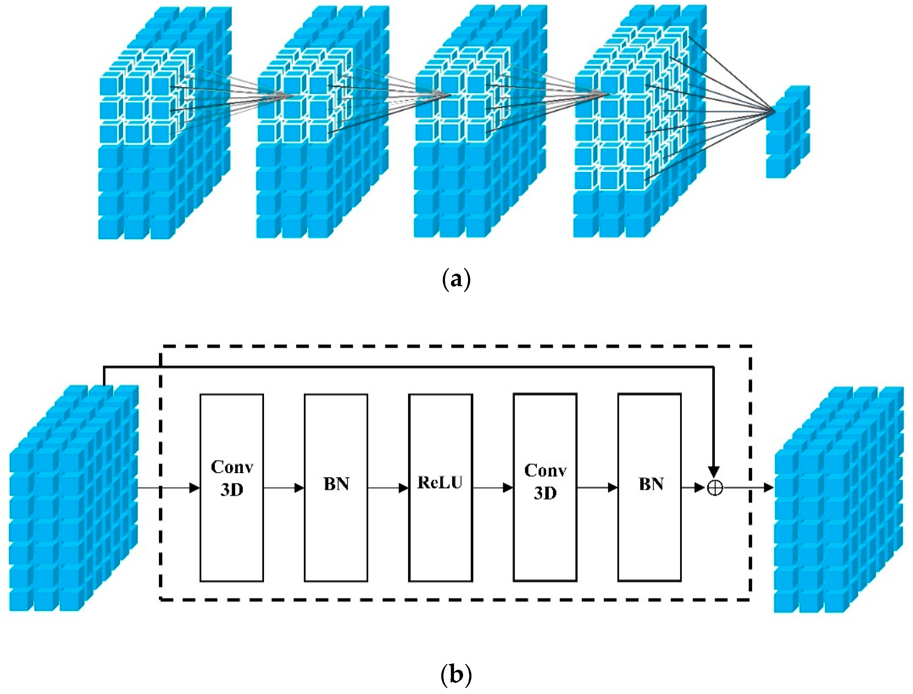
From a global perspective, we constructed three K-layers 3D CNN based on MTL to extract features from closeness, period and trend, respectively. Concretely, as illustrated in Figure 4a, we take trends as an example, in order to capture patterns in historical data. The constructed K-layers 3D CNN which successively took and as input tensors, and followed by convolution as:
where denotes the convolutional operation; is a batch normalization operation [48] followed by an activation function, that is, ; and are learnable parameters in layer ; and is or .
4.3. Feature Embedding Component
Based on the 3D CNN, we got six feature tensors which can be view as time series. To fusion the features of three parts of historical data, we proposed using long short-term memory (LSTM) based on attention mechanism to encoding feature tensors into another tensor. LSTM [49] is a type of recurrent neural network architecture, which is good at processing time series. It was proposed to address the problem of gradient vanishing or exploding of classic Recurrent Neural Network (RNN).
As shown in Figure 2, in each time interval , the output of 3D CNN was taken as the input of LSTM after flattening. The peculiar thing about LSTM is that it has a memory cell and three gates, that is, a forget gate, an input gate, and an output gate. Specifically, the function of the memory cell is to store information, the forget gate decides what information is going to throw from the cell, the input gate determines what information will be added to the cell, and the output gate controls what information is sent to next time interval. In detail, at time interval , the input and output vector at the previous interval are first sent into the forget gate to obtain the forget gate’s activation vector . Next, the input gate combines and to calculate its activation vector . Then we can update memory cell into according to the above all activation vectors and the memory cell state vector at previous time interval. Afterward, and are used to obtain the output gate’s activation vector Finally, we can get the output vector at this time interval through and . Formally, the updating equations for LSTM are provided below:
where is the Hadamard product, is hyperbolic tangent function, and is sigmoid function. Different kernel matrices and bias are parameters to be learned.
After the LSTM generated hidden states from the inputs , in order to capture the interaction between taxi pick-up and taxi drop-off at different time intervals, we decoded the six hidden states based on the attention mechanism and generated six new representation vectors. As illustrated in the dashed box in the middle of Figure 2 for each timestamp , we first calculated the extent of importance between each hidden state and the previous output of the decoder LSTM, then normalized it into , and finally calculated the weighted sum of and to get which sent into the next timestamp. The key formula for decoding the hidden state is as follows:
where is a one-dimensional convolutional network that is trained with all the other components of the proposed system.
We then aimed to capture the correlation between taxi demand for pick-up and drop. In order to address the issue that the deeper networks are difficult to train, He et al. [50] proposed a residual learning framework named ResNet. In this study, we captured the aforementioned correlation by 3D ResNet. Firstly, reshaped the six representation vectors that come from the attention-based LSTM into matrices, and then stacked them into a tensor . Secondly, we took as the input of stacked 3D residual units, as shown in Figure 4b, which is defined as follows:
where is the 3D residual units, is learnable parameter. Finally, we flattened the output of 3D ResNet into a final representation vector .
4.4. External Factors Component
Taxi demand can also be affected by many complex external factors, such as weather, date, region functions, and regional public transport conditions. Intuitively, taxi demand may be affected by the weather a lot, with people more inclined to take a taxi when it’s raining, and walking when it’s sunny. Similarly, the date and time will also affect taxi demand. We may have a fixed travel routes on weekdays and working hours while having various choices on weekends and holidays. Of equal importance, the public transportation system will influence travel habits of people due to its convenience and safety.
In this study, there are mainly three types of external data: (1) Numerical data, for example, wind speed, temperature or humidity; (2) categorical data, for example, day of the week, holiday, or weather; (3) graph data, for example, metro information. For numerical data, we directly normalized them and stacked them into a vector . For categorical data, we conducted one-hot coding for them and concatenated them into another vector .
As for graph data, we constructed an undirected graph , where the set of grids are nodes , is the edge set, and indicates the distance between every two nodes. In this study, we simply used Manhattan distance to measure the distance between two nodes. Note that if the two nodes could be directly reached by metro, we set to 1; if the two nodes could be reached through a transfer, we set to 2, and so on. Based on that, the distance between a metro station and the eight grids surrounding another metro station is set to . Thus, we ended up with a fully connected graph, and for all the nodes, the closer to other nodes, the more convenient the traffic will be. Afterward, we applied Large-scale Information Network Embedding (LINE) algorithm [51] embedding graph into a vector .
At last, we fused the above vectors into a new vector which then fed into a two-layers fully-connected neural network, and obtained the representation of external factors at time interval . More specifically, we defined
where is Hadamard product, denotes concatenation operator, is a two-layers fully-connected neural network, and , and are the learnable parameters.
4.5. Prediction Component
Based on feature encoding and external information encoding, then we aimed to predict the taxi demand in the next interval. We concatenated the output of feature encoding with the output of the external information:
where denotes concatenation operator, and . Then we fed to the fully connected network to get the final prediction value . Formally, the prediction function is provided as below:
where and are learnable parameters, and is the ReLU function.
Previous studies mostly take the loss as the loss function, yet the loss is sensitive to outliers; the gradient of loss is high for larger loss values and vice versa. On the contrary, the loss is robust to outliers, but its gradient is the same throughout even for small loss values; meanwhile, discontinuous derivatives would decrease efficiency in problem-solving. Despite taxi demands being generally stable, outliers still may occur due to various reasons; for example, a sudden rainstorm, concerts, or public events. Thus, we combined loss and loss to train Taxi3D by minimizing the Smooth L1 loss [52]. The loss function we used is defined as:
in which
where denotes all the learnable parameters, is the numbers of all predicted values.
5. Experiment and Discussion
5.1. Dataset
In this paper, we used a real dataset collected from Didi Chuxing [53]; it consists of five million taxi trips records in Chengdu from 1 October 2016 to 31 December 2016. The size of the area to be predicted was about . There were about 168,362 demands (including pick-up and drop-off) each day on average. Each row of the original data can be seen as a tuple (order ID, pick-up time, pick-up longitude, pick-up latitude, drop-off time, drop-off longitude, drop-off latitude), and we processed the original data with the method mentioned in Section 3 to obtain the final dataset.
The external factors including meteorological features (e.g., weather condition, wind speed), temporal features (e.g., day of the week, hour of the day, holiday) and spatial features (e.g., public transport conditions). Taking 10:00 a.m. on 7 October 2016 as an example, we selected the following features: Sunny, wind speed, temperature, probability of precipitation, humidity, Friday, the 21st time interval, holiday (Chinese National Day holiday), and metro information.
5.2. Experimental Settings
The data from 1 October 2016 to 18 November 2016 (49 days) was used for training, validation data was from 19 November 2016 to 23 November 2016 (5 days), and the remaining 7 days of data were used for testing. In our experiment, we firstly trained our model on training data, and validation data was used to early-stop our algorithm. Afterward, we continued training our model on the training data and validation data for a fixed number of epochs. For fair comparison, other methods were also trained like this.
In our experiment, we set time interval to 30 min, that is, . Limited by the dataset, we set and , thus, we got grids for which each grid is about . All these experiments were run on the server with NVIDIA Tesla K40M. We used Adam [54] for optimization. We used PyTorch [55] to implement our proposed model.
We set filters of size in all convolutional operation. For the length of closeness, period and trend, we searched , and . We searched (the number of layers of 3D CNN) and (the number of stacked 3D ResNet) from 2 to 6.
5.3. Baselines
To be fair, we present the best performance of each method. The proposed model and its variants were trained by multi-task learning. For other baselines, we used taxi pick-up data, taxi drop-off data and all data for training and prediction. Specifically, we compared our model with the following baselines:
- Historical average (HA): By simply averaging the values of previous taxi pick-up and taxi drop-off demands at the same location and the same time interval, we can get the predicted value.
- Autoregressive integrated moving average (ARIMA): ARIMA is a well-known model for predicting times series.
- XGBoost: XGBoost is a well-known powerful model and is widely used by data scientists to achieve state-of-the-art results on many machine learning challenges [56].
- Multiple layer perceptron (MLP): We compared our model with an MLP which consisted of 4 hidden layers. Each layer had 128, 128, 128, and 64 hidden units, respectively.
- Long Short-Term Memory: LSTM is a special kind of RNN, capable of learning long-term dependencies, and it is widely used in time series processing.
- ST-ResNet [8]: ST-ResNet is an end-to-end traffic prediction approach based on deep learning, which uses the residual network to capture the spatial and temporal characteristics of crowd traffic, and also combines with external factors.
For fair comparison, all the methods above were implemented with the same equipment and environment. We also compared the effects of different components of the proposed model.
- Taxi3D-single: To verify the effectiveness of MTL, in this variant, we designed two independent networks which extracted spatiotemporal features from taxi pick-up data and drop-off data respectively. We then stacked the outputs and fed them into the feature embedding component as Taxi3D does.
- Taxi3D-lstm: In this variant, we fed the output of the multi-task spatiotemporal feature extraction component into the LSTM for predicting.
- Taxi3D-na: Taxi3D without attention-based LSTM; we simply reshaped the output of Figure 2a and stacked them into tensor, which was taken as the input of 3D ResNet.
- Taxi3D-nr: We used a 4-layers 3D CNN instead of 3D ResNet in feature embedding component.
- Taxi3D-ne: This variant removes the external factors component.
5.4. Evaluation Metric
We evaluated our method by root mean square error (RMSE) as:
where is the predict value, is the real value, and is numbers of all predicted values.
5.5. Tuning Hyperparameters
Tuning closeness, period and trend. In this section, we verify the effect of the length of closeness, period and trend, that is, , and . Note that we fixed and . In the first place, we set and , and tuned . As shown in Figure 5, we saw RMSE first decrease, then reach the minimum value when , and finally increase. Thus, we set . In the second place, we fixed , and started to tune . Figure 5 illustrates the results, when started with 1, RMSE gradually decreased and reached the lowest point at 3, then started to gradually increase. Thus, we determined as 3. After fixing , , we aimed to tune . When , we got the minimum RMSE. From this, we saw that the time interval closest to the predicted time interval had the most significant influence on the result. Meanwhile, demand situations at the same time yesterday and last week were also slightly helpful to enhance performance. However, the less data, the faster the computation, and we needed to make a trade-off between efficiency and accuracy.
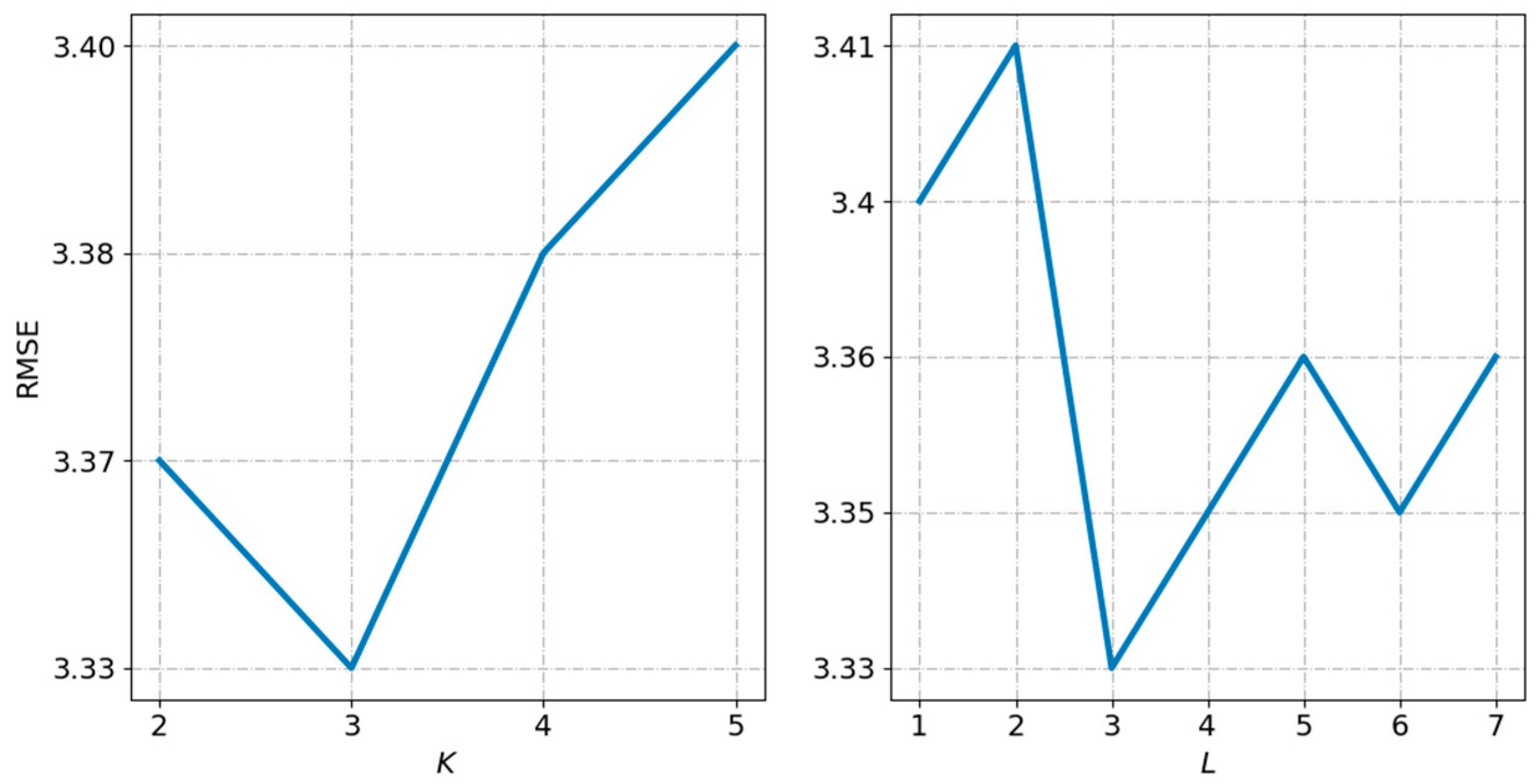
Tuning the number of layers of 3D CNN. The role of 3D CNN in the multi-task spatiotemporal feature extraction component is to capture spatiotemporal correlation. In this section, we compare the model effects of 3D CNN with different layers. As we can see from Figure 6, when was between 2 to 3, RMSE decreased. When , RMSE reached the minimum value, and then increased with the increase of . Thus, we set in this study.
Tuning the number of stacked 3D ResNet. We utilized 3D ResNet to capture the correlation between taxi pick-up and taxi drop-off. We here verify the impact of number of layers of 3D ResNet. As shown in Figure 6, we observed that when , the model showed the best performance. One possible reason is that, limited by the amount of data, it is not that the deeper the network, the more it learns. Our 3D ResNet does not require very deep networks.
5.6. Model Comparsion
First, we aimed to compare our model with the baselines from the perspective of RMSE. The results are shown in Table 1. We can see that our model achieved the lowest RMSE among all the models. To be specific, MLP performed poorly (i.e., RMSE was 4.81, 5.48, and 5.31, respectively), as the method did not take spatiotemporal correlations into account. HA, ARIMA, and LSTM considered temporal correlation and achieved better results. As a powerful boosting tree-based model, XGBoost presented good performance, but this method also does not deal with spatial correlation. The good performance of ST-ResNet shows the effectiveness of the method combined with spatiotemporal information. However, this method separates the correlation between temporal correlation and spatial correlation. In a nutshell, the RMSE of our model was 3.33, which achieves relatively 5.93% up to 37.29% lower RMSE than other baselines.
5.7. Variants Comparsion
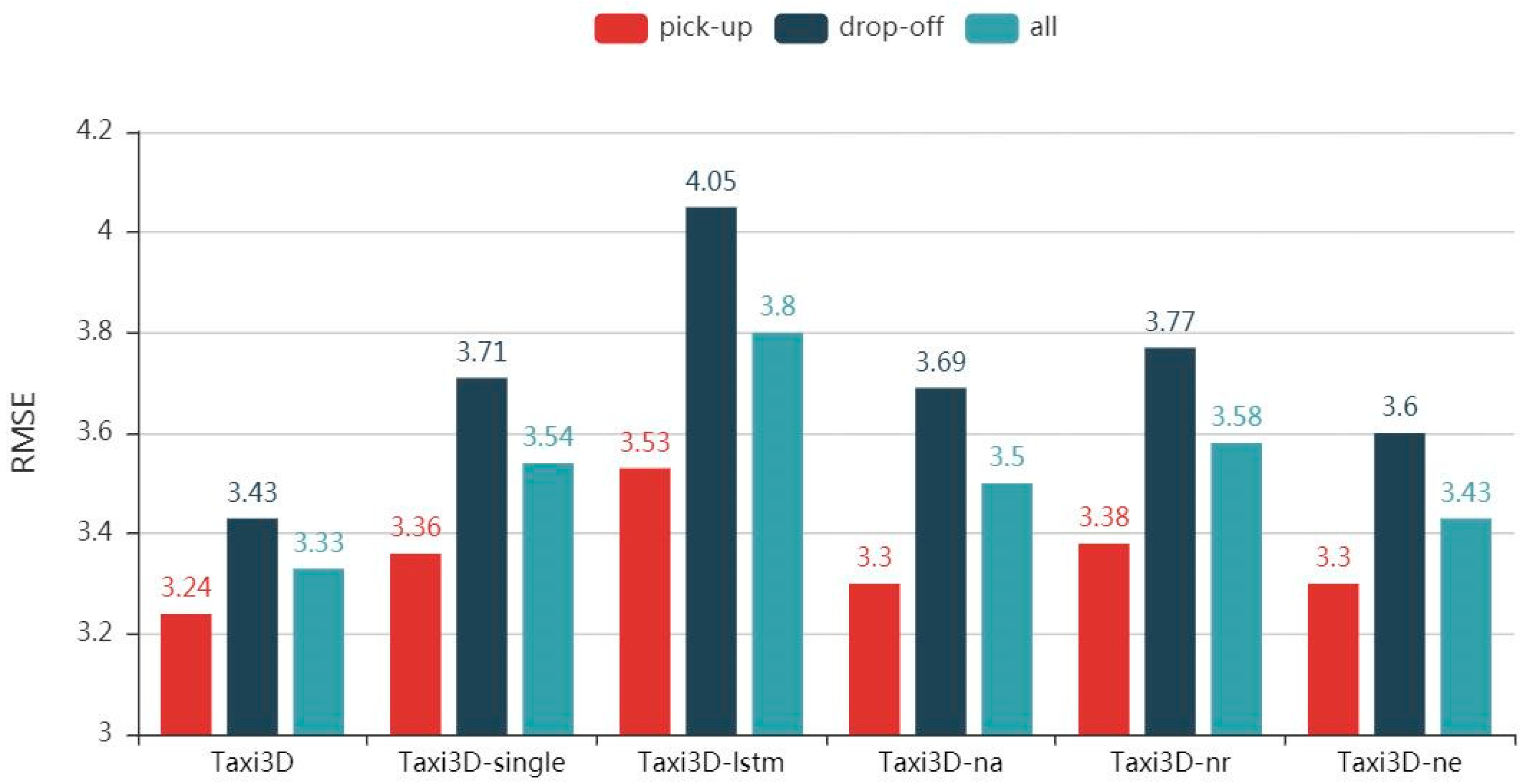
To evaluate the importance of each component of the proposed model, in this section, we decompose Taxi3D into various variants and conduct comparison experiments. The results are presented in Figure 7.
Effectiveness of MTL. Instead of extracting spatiotemporal features in the same network, we designed two identical but independent 3D CNN in Taxi3D-single, which means the increase in the number of parameters and the decrease of computational efficiency. We observed that multi-task learning accordingly improves model performance by 3.7%, 8.2%, and 5.9% in two related tasks and all data, compared with RMSE 3.36, 3.71 and 3.54 obtained by Taxi3D-single.
One potential reason is that the tasks of predicting taxi demand for pick-up and drop-off are related, and we can extract common spatiotemporal features from them by sharing information. In fact, deep learning models require millions of data points to train; limited by data and computing power, many applications cannot satisfy this requirement. Thus, we may take advantage of useful information from other related tasks to assist in the training of our model. In our study, the multi-task learning component is equivalent to increasing the amount of training data and sharing useful information at the same time. As a result, Taxi3D achieved better performance than Taxi3D-single.
Effectiveness of Feature Embedding Component. As previously mentioned, feature vectors extracted by the MTL component can be viewed as time series. Thus, we retained the MTL component and replaced other parts with LSTM, that is, Taxi3D-lstm. The results indicate that the performance of the model decreased significantly.
The role of the MTL component is to extract temporal and spatial features without separating temporal correlation and spatial correlation. The six vectors generated by the MTL component are the spatiotemporal features of taxi pick-up and taxi drop-off in the three time periods of closeness, period and trend, respectively. Despite treating these vectors as time series having limited effect, the information contained in the spatiotemporal features still needs to be further processed. Also, this variant does not capture the correlation between taxi demand for pick-up and drop-off, which may interact with each other.
Effectiveness of Attention-based LSTM. Due to the above reasons, we then used 3D ResNet to further process the spatiotemporal features; that is, adding 3D ResNet to the back of the MTL component instead of LSTM. The results showed that the performance improvement of Taxi3D-na is limited compared with Taxi3D-LSTM. Concretely, compare with the RMSE of 3.53, 4.05 and 3.8 obtained by Taxi3D-LSTM, Taxi3D-na accordingly improved performance by 6.5%, 8.9%, and 7.9% in two related tasks and all data.
The possible reason is that although Taxi3D-na captured correlation between pick-up and drop-off, the method which simply stacked spatiotemporal features may be questionable. Technically, the LSTM is a master of processing time series. The attention mechanism mimics the way people focus on critical information while ignoring the rest. Thus we combined LSTM and attention mechanism to fuse spatiotemporal features of historical demands, which is equivalent to feature embedding. Among them, the LSTM captures the temporal correlation, and the attention mechanism assigns weights to the six spatiotemporal features when generating the new representations of historical data.
Effectiveness of 3D ResNet. We then compared Taxi3D-nr with Taxi3D, in which the former replaces the 3D-ResNet with plain 3D CNN. Even though we used attention-based LSTM to fuse the spatiotemporal feature, plain 3D CNN may not capture spatial and temporal correlation well, and the RMSE of Taxi3D-nr was 4.1%, 5% and 7% than that of 3.24, 3.43 and 3.33 obtained by Taxi3D, respectively.
With the increase of the layers of neural networks, there may be obstacles, such as information loss, gradient vanishing, gradient exploding and so on when the transmitting information, which leads to difficulty in training deep networks. Therefore, we utilized ResNet to increase the network depth to capture the correlation between pick-up and drop-off.
Effectiveness of External Factors Component. As illustrated in Figure 7, Taxi3D achieved better performance than Taxi3D-ne. The results show that the addition of the external component boosts predictive performance. Intuitively, external factors will affect taxi demand, since human behavior has a lot to do with the environment. For example, the travel habits of people on weekends and holidays may be quite different from the working day, lousy weather increases taxi demands and good weather may make walking more enjoyable.
6. Conclusions and Future Work
In this paper, we studied the problem of predicting taxi demand for pick-up and drop-off, and we proposed a novel deep-learning based model. We evaluated our model on the real taxi demand data in Chengdu, and the results showed that RMSE of 3.33 obtained by our model achieved relatively 5.93% up to 37.29% lower RMSE than other baselines. The main contribution of this paper was to propose an innovative learning framework to predict taxi demand. In the first level, we deemed the demand situation of the urban taxi as a video and utilized 3D CNN combined with MTL to extract spatiotemporal features. In the second level, we used attention-based LSTM for feature embedding and combined with 3D ResNet to capture the correlation between pick-up and drop-off. Then we fused external factors and made the prediction.
The study concludes that, from the perspective of spatial correlation, the demand for taxis between adjacent regions will influence each other. From the standpoint of temporal correlation, taxi demand in adjacent periods may affect each other, and the demand at the same time interval is nearly similar. In terms of spatiotemporal correlation, they complement each other and should not be separated, and taxi pick-up and taxi drop-off will also affect each other. From the citizen’s point of view, the weather, holidays, and public transport conditions have an impact on taxi demand.
However, our study still has limitations. In the future, we will consider the following aspects to improve prediction accuracy: The first is to improve the predicting performance of hot spots with the help of time series anomaly detection algorithms. Hot spots are prone to outliers, which have a significant impact on model training and prediction performance. The second is to divide the city according to regional semantics, and then predict taxi demand by graph convolutional networks. In real life, the interior of a city will likely be irregular rather than square. Also, we will consider extending our model to multi-step prediction.
Author Contributions
Conceptualization, L.K., X.Y. (Xuejin Yan) and X.Y. (Xiaoxian Yang); funding acquisition, L.K.; methodology, L.K., X.Y. (Xuejin Yan) and X.Y. (Xiaoxian Yang); project administration, L.K.; resources, L.K.; software, X.Y. (Xuejin Yan) and X.T.; supervision, L.K. and X.Y. (Xiaoxian Yang); validation, L.K., X.T. and X.Y. (Xiaoxian Yang); visualization, S.L.; writing—original draft, X.Y. (Xuejin Yan) and S.L.; writing—review & editing, L.K., X.Y. (Xuejin Yan), X.T., S.L. and X.Y. (Xiaoxian Yang).
Funding
The research is supported by the National Natural Science Foundation of China (No.61772560), the National Key R&D Program of China (No.2018YFB1003800), and the Natural Science Foundation of Hunan Province (No. 2019JJ40388).
Acknowledgments
Data retrieved from Didi Chuxing.
Conflicts of Interest
The authors declare no conflict of interest.
References
- Williams, B.M.; Hoel, L.A. Modeling and forecasting vehicular traffic flow as a seasonal ARIMA process: Theoretical basis and empirical results. J. Transp. Eng. 2003, 129, 664–672. [Google Scholar] [CrossRef]
- Shekhar, S.; Williams, B. Adaptive seasonal time series models for forecasting short-term traffic flow. Transp. Res. Rec. J. Transp. Res. Board 2008, 2024, 116–125. [Google Scholar] [CrossRef]
- Moreira-Matias, L.; Gama, J.; Ferreira, M.; Mendes-Moreira, J.; Damas, L. Predicting taxi–passenger demand using streaming data. IEEE Trans. Intell. Transp. Syst. 2013, 14, 1393–1402. [Google Scholar] [CrossRef]
- LeCun, Y.; Bengio, Y.; Hinton, G. Deep learning. Nature 2015, 521, 436. [Google Scholar] [CrossRef]
- Lv, Y.; Duan, Y.; Kang, W.; Li, Z.; Wang, F.-Y. Traffic flow prediction with big data: A deep learning approach. IEEE Trans. Intell. Transp. Syst. 2015, 16, 865–873. [Google Scholar] [CrossRef]
- Ma, X.; Yu, H.; Wang, Y.; Wang, Y. Large-scale transportation network congestion evolution prediction using deep learning theory. PLoS ONE 2015, 10, e0119044. [Google Scholar] [CrossRef] [PubMed]
- Zhang, J.; Zheng, Y.; Qi, D.; Li, R.; Yi, X. DNN-based prediction model for spatio-temporal data. In Proceedings of the 24th ACM SIGSPATIAL International Conference on Advances in Geographic Information Systems, Burlingame, CA, USA, 31 October–3 Novembe 2016; p. 92. [Google Scholar]
- Zhang, J.; Zheng, Y.; Qi, D. Deep Spatio-Temporal Residual Networks for Citywide Crowd Flows Prediction. In Proceedings of the AAAI, San Francisco, CA, USA, 4–9 February 2017; pp. 1655–1661. [Google Scholar]
- Zhao, Z.; Chen, W.; Wu, X.; Chen, P.C.; Liu, J. LSTM network: A deep learning approach for short-term traffic forecast. IET Intell. Transp. Syst. 2017, 11, 68–75. [Google Scholar] [CrossRef]
- Xu, J.; Rahmatizadeh, R.; Bölöni, L.; Turgut, D. Real-time prediction of taxi demand using recurrent neural networks. IEEE Trans. Intell. Transp. Syst. 2018, 19, 2572–2581. [Google Scholar] [CrossRef]
- Wu, Y.; Tan, H. Short-Term Traffic Flow Forecasting with Spatial–Temporal Correlation in a Hybrid Deep Learning Framework. Available online: https://arxiv.org/pdf/1612.01022.pdf (accessed on 28 May 2019).
- Yu, H.; Wu, Z.; Wang, S.; Wang, Y.; Ma, X. Spatiotemporal recurrent convolutional networks for traffic prediction in transportation networks. Sensors 2017, 17, 1501. [Google Scholar] [CrossRef]
- Yao, H.; Wu, F.; Ke, J.; Tang, X.; Jia, Y.; Lu, S.; Gong, P.; Ye, J.; Li, Z. Deep multi-view spatial-temporal network for taxi demand prediction. In Proceedings of the Thirty-Second AAAI Conference on Artificial Intelligence, New Orleans, LA, USA, 2–7 February 2018. [Google Scholar]
- Yin, Y.; Chen, L.; Wan, J. Location-aware service recommendation with enhanced probabilistic matrix factorization. IEEE Access 2018, 6, 62815–62825. [Google Scholar] [CrossRef]
- Yin, Y.; Aihua, S.; Min, G.; Yueshen, X.; Shuoping, W. QoS prediction for web service recommendation with network location-aware neighbor selection. Inter. J. Softw. Eng. Knowl. Eng. 2016, 26, 611–632. [Google Scholar] [CrossRef]
- Yin, Y.; Xu, Y.; Xu, W.; Gao, M.; Yu, L.; Pei, Y. Collaborative service selection via ensemble learning in mixed mobile network environments. Entropy 2017, 19, 358. [Google Scholar] [CrossRef]
- Gao, H.; Miao, H.; Liu, L.; Kai, J.; Zhao, K. Automated quantitative verification for service-based system design: A visualization transform tool perspective. Inter. J. Softw. Eng. Knowl. Eng. 2018, 28, 1369–1397. [Google Scholar] [CrossRef]
- Gao, H.; Zhang, K.; Yang, J.; Wu, F.; Liu, H. Applying improved particle swarm optimization for dynamic service composition focusing on quality of service evaluations under hybrid networks. Inter. J. Distrib. Sensor Netw. 2018, 14, 1550147718761583. [Google Scholar] [CrossRef]
- Gao, H.; Mao, S.; Huang, W.; Yang, X. Applying Probabilistic Model Checking to Financial Production Risk Evaluation and Control: A Case Study of Alibaba’s Yu’e Bao. IEEE Trans. Comput. Soc. Syst. 2018, 5, 785–795. [Google Scholar] [CrossRef]
- Gao, H.; Chu, D.; Duan, Y.; Yin, Y. Probabilistic model checking-based service selection method for business process modeling. Inter. J. Softw. Eng. Knowl. Eng. 2017, 27, 897–923. [Google Scholar] [CrossRef]
- Gao, H.; Huang, W.; Yang, X.; Duan, Y.; Yin, Y. Toward service selection for workflow reconfiguration: An interface-based computing solution. Future Gener. Comput. Syst. 2018, 87, 298–311. [Google Scholar] [CrossRef]
- De, G.; Gao, W. Forecasting China’s Natural Gas Consumption Based on AdaBoost-Particle Swarm Optimization-Extreme Learning Machine Integrated Learning Method. Energies 2018, 11, 2938. [Google Scholar] [CrossRef]
- Li, C.; Zheng, X.; Yang, Z.; Kuang, L. Predicting Short-Term Electricity Demand by Combining the Advantages of Arma and Xgboost in Fog Computing Environment. Available online: https://www.hindawi.com/journals/wcmc/2018/5018053/ (accessed on 28 May 2019).
- Kuang, L.; Yu, L.; Huang, L.; Wang, Y.; Ma, P.; Li, C.; Zhu, Y. A personalized qos prediction approach for cps service recommendation based on reputation and location-aware collaborative filtering. Sensors 2018, 18, 1556. [Google Scholar] [CrossRef] [PubMed]
- Yin, Y.; Xu, W.; Xu, Y.; Li, H.; Yu, L. Collaborative QoS Prediction for Mobile Service with Data Filtering and SlopeOne Model. Available online: https://www.hindawi.com/journals/misy/2017/7356213/ (accessed on 28 May 2019).
- Deng, S.; Xiang, Z.; Yin, J.; Taheri, J.; Zomaya, A.Y. Composition-driven IoT service provisioning in distributed edges. IEEE Access 2018, 6, 54258–54269. [Google Scholar] [CrossRef]
- Chen, Y.; Deng, S.; Ma, H.; Yin, J. Deploying Data-Intensive Applications with Multiple Services Components on Edge. Available online: https://doi.org/10.1007/s11036-019-01245-3 (accessed on 28 May 2019).
- Deng, S.; Huang, L.; Xu, G.; Wu, X.; Wu, Z. On deep learning for trust-aware recommendations in social networks. IEEE Trans. Neural Netw. Learn. Syst. 2016, 28, 1164–1177. [Google Scholar] [CrossRef]
- Yin, Y.; Chen, L.; Xu, Y.; Wan, J.; Zhang, H.; Mai, Z. QoS Prediction for Service Recommendation with Deep Feature Learning in Edge Computing Environment. Available online: https://doi.org/10.1007/s11036-019-01241-7 (accessed on 28 May 2019).
- Gao, H.; Duan, Y.; Miao, H.; Yin, Y. An approach to data consistency checking for the dynamic replacement of service process. IEEE Access 2017, 5, 11700–11711. [Google Scholar] [CrossRef]
- Padmanabhan, J.; Johnson Premkumar, M.J. Machine learning in automatic speech recognition: A survey. IETE Tech. Rev. 2015, 32, 240–251. [Google Scholar] [CrossRef]
- Fei, H.; Tan, F. Bidirectional Grid Long Short-Term Memory (BiGridLSTM): A Method to Address Context-Sensitivity and Vanishing Gradient. Algorithms 2018, 11, 172. [Google Scholar] [CrossRef]
- Siniscalchi, S.M.; Salerno, V.M. Adaptation to new microphones using artificial neural networks with trainable activation functions. IEEE Trans. Neural Net. Learn. Syst. 2016, 28, 1959–1965. [Google Scholar] [CrossRef]
- Zhang, Y.; Yang, Q. An overview of multi-task learning. Natl. Sci. Rev. 2017, 5, 30–43. [Google Scholar] [CrossRef] [Green Version]
- Hamed, M.M.; Al-Masaeid, H.R.; Said, Z.M.B. Short-term prediction of traffic volume in urban arterials. J.Transp. Eng. 1995, 121, 249–254. [Google Scholar] [CrossRef]
- Van Der Voort, M.; Dougherty, M.; Watson, S. Combining Kohonen maps with ARIMA time series models to forecast traffic flow. Transp. Res. Part. C Emerg. Tech. 1996, 4, 307–318. [Google Scholar] [CrossRef]
- Williams, B. Multivariate vehicular traffic flow prediction: Evaluation of ARIMAX modeling. Transp. Res. Rec. J. Transp. Res. Board 2001, 1776, 194–200. [Google Scholar] [CrossRef]
- Wu, C.-H.; Ho, J.-M.; Lee, D.-T. Travel-time prediction with support vector regression. IEEE Trans. Intell. Transp. Syst. 2004, 5, 276–281. [Google Scholar] [CrossRef]
- Zheng, W.; Lee, D.-H.; Shi, Q. Short-term freeway traffic flow prediction: Bayesian combined neural network approach. J. Transp. Eng. 2006, 132, 114–121. [Google Scholar] [CrossRef]
- Kuang, L.; Yan, H.; Zhu, Y.; Tu, S.; Fan, X. Predicting duration of traffic accidents based on cost-sensitive Bayesian network and weighted K-nearest neighbor. J. Intell. Transp. Syst. 2019, 23, 161–174. [Google Scholar] [CrossRef]
- Chang, H.; Lee, Y.; Yoon, B.; Baek, S. Dynamic near-term traffic flow prediction: Systemoriented approach based on past experiences. IET Intell. Transp. Syst. 2012, 6, 292–305. [Google Scholar] [CrossRef]
- Xia, D.; Wang, B.; Li, H.; Li, Y.; Zhang, Z. A distributed spatial–temporal weighted model on MapReduce for short-term traffic flow forecasting. Neurocomputing 2016, 179, 246–263. [Google Scholar] [CrossRef]
- Sutskever, I.; Vinyals, O.; Le, Q.V. Sequence to sequence learning with neural networks. In Proceedings of the Advances in Neural Information Processing Systems, Montréal, QC, Canada, 8–13 December 2014; pp. 3104–3112. [Google Scholar]
- Zhou, X.; Shen, Y.; Zhu, Y.; Huang, L. Predicting multi-step citywide passenger demands using attention-based neural networks. In Proceedings of the Eleventh ACM International Conference on Web Search and Data Mining, Marina Del Rey, CA, USA, 5–9 February 2018; pp. 736–744. [Google Scholar]
- Ji, S.; Xu, W.; Yang, M.; Yu, K. 3D convolutional neural networks for human action recognition. IEEE Trans. Pattern Anal. Mach. Intell. 2013, 35, 221–231. [Google Scholar] [CrossRef]
- Tran, D.; Bourdev, L.; Fergus, R.; Torresani, L.; Paluri, M. Learning spatiotemporal features with 3d convolutional networks. In Proceedings of the IEEE International Conference on Computer Vision, Boston, MA, USA, 7–12 June 2015; pp. 4489–4497. [Google Scholar]
- Yosinski, J.; Clune, J.; Nguyen, A.; Fuchs, T.; Lipson, H. Understanding Neural Networks through Deep Visualization. Available online: https://arxiv.org/abs/1506.06579 (accessed on 28 May 2019).
- Ioffe, S.; Szegedy, C. Batch normalization: Accelerating deep network training by reducing internal covariate shift. In Proceedings of the 32nd International Conference on Machine Learning, Lille, France, 6 –11 July 2015; pp. 448–456. [Google Scholar]
- Hochreiter, S.; Schmidhuber, J. Long short-term memory. Neural Comput. 1997, 9, 1735–1780. [Google Scholar] [CrossRef]
- He, K.; Zhang, X.; Ren, S.; Sun, J. Deep residual learning for image recognition. In Proceedings of the IEEE Conference on Computer Vision and Pattern Recognition, Las Vegas, NV, USA, 27–30 June 2016; pp. 770–778. [Google Scholar]
- Tang, J.; Qu, M.; Wang, M.; Zhang, M.; Yan, J.; Mei, Q. Line: Large-scale information network embedding. In Proceedings of the 24th International Conference on World Wide Web, Florence, Italy, 18–22 May 2015; pp. 1067–1077. [Google Scholar]
- Girshick, R. Fast r-cnn. In Proceedings of the IEEE International Conference on Computer Vision, Santiago, Chile, 13–16 December 2015; pp. 1440–1448. [Google Scholar]
- Didi Chuxing. Available online: https://gaia.didichuxing.com (accessed on 16 December 2018).
- Kingma, D.P.; Ba, J. Adam: A method for stochastic optimization. In Proceedings of the 3rd International Conference for Learning Representations, San Diego, CA, USA, 7–9 May 2015. [Google Scholar]
- Paszke, A.; Gross, S.; Chintala, S.; Chanan, G.; Yang, E.; DeVito, Z.; Lin, Z.; Desmaison, A.; Antiga, L.; Lerer, A. Automatic differentiation in pytorch. In Proceedings of the Future of Gradient-Based Machine Learning Software and Techniques (Autodiff) in Thetwenty-Ninth Annual Conference on Neural Information Processingsystems (NIPS), Long Beach, CA, USA, 4–9 December 2017. [Google Scholar]
- Chen, T.; Guestrin, C. Xgboost: A scalable tree boosting system. In Proceedings of the 22nd ACM Sigkdd International Conference on Knowledge Discovery and Data Mining, San Francisco, CA, USA, 13–17 August 2016; pp. 785–794. [Google Scholar]
Figure 1.
Regions in Chengdu: (a) Partition in spatial view; (b) partition in temporal view.

Figure 2.
Architecture of the proposed model Taxi3D.

Figure 3.
The demand in three distinct areas of Chengdu. All data has been normalized: (a) Grid (1, 2) is near schools, residential; (b) grid (11,3) is near a university and shopping malls; (c) grid (3, 2) is near office buildings, shopping malls.
Figure 3.
The demand in three distinct areas of Chengdu. All data has been normalized: (a) Grid (1, 2) is near schools, residential; (b) grid (11,3) is near a university and shopping malls; (c) grid (3, 2) is near office buildings, shopping malls.


Figure 4.
3D convolution and 3D Residual Unit: (a) 3D convolution; (b) 3D Residual Unit.

Figure 5.
Tuning the length of closeness, period and trend.

Figure 6.
Tuning the number of layers.

Figure 7.
Performance comparison among different variants.


Table 1.
Performance comparison among different methods.
| Method | RMSE | ||
|---|---|---|---|
| Pick-up | Drop-off | All | |
| MLP | 4.81 | 5.48 | 5.31 |
| HA | 3.88 | 4.32 | 4.11 |
| ARIMA | 4.09 | 4.15 | 4.13 |
| XGBoost | 3.58 | 3.85 | 3.84 |
| LSTM | 3.76 | 4.19 | 4.00 |
| ST-ResNet | 3.54 | 3.72 | 3.54 |
| Taxi3D | 3.24 | 3.43 | 3.33 |
| Taxi3D-single | 3.36 | 3.71 | 3.54 |
| Taxi3D-lstm | 3.53 | 4.05 | 3.80 |
| Taxi3D-na | 3.30 | 3.69 | 3.50 |
| Taxi3D-nr | 3.38 | 3.77 | 3.58 |
| Taxi3D-ne | 3.30 | 3.60 | 3.45 |
© 2019 by the authors. Licensee MDPI, Basel, Switzerland. This article is an open access article distributed under the terms and conditions of the Creative Commons Attribution (CC BY) license (http://creativecommons.org/licenses/by/4.0/).
Share and Cite
MDPI and ACS Style
Kuang, L.; Yan, X.; Tan, X.; Li, S.; Yang, X. Predicting Taxi Demand Based on 3D Convolutional Neural Network and Multi-task Learning. Remote Sens. 2019, 11, 1265. https://doi.org/10.3390/rs11111265
AMA Style
Kuang L, Yan X, Tan X, Li S, Yang X. Predicting Taxi Demand Based on 3D Convolutional Neural Network and Multi-task Learning. Remote Sensing. 2019; 11(11):1265. https://doi.org/10.3390/rs11111265
Chicago/Turabian StyleKuang, Li, Xuejin Yan, Xianhan Tan, Shuqi Li, and Xiaoxian Yang. 2019. "Predicting Taxi Demand Based on 3D Convolutional Neural Network and Multi-task Learning" Remote Sensing 11, no. 11: 1265. https://doi.org/10.3390/rs11111265
Note that from the first issue of 2016, this journal uses article numbers instead of page numbers. See further details here.