Dual Learning-Based Siamese Framework for Change Detection Using Bi-Temporal VHR Optical Remote Sensing Images

Abstract

As a fundamental and profound task in remote sensing, change detection from very-high-resolution (VHR) images plays a vital role in a wide range of applications and attracts considerable attention. Current methods generally focus on the research of simultaneously modeling and discriminating the changed and unchanged features. In practice, for bi-temporal VHR optical remote sensing images, the temporal spectral variability tends to exist in all bands throughout the entire paired images, making it difficult to distinguish none-changes and changes with a single model. In this paper, motivated by this observation, we propose a novel hybrid end-to-end framework named dual learning-based Siamese framework (DLSF) for change detection. The framework comprises two parallel streams which are dual learning-based domain transfer and Siamese-based change decision. The former stream is aimed at reducing the domain differences of two paired images and retaining the intrinsic information by translating them into each other’s domain. While the latter stream is aimed at learning a decision strategy to decide the changes in two domains, respectively. By training our proposed framework with certain change map references, this method learns a cross-domain translation in order to suppress the differences of unchanged regions and highlight the differences of changed regions in two domains, respectively, then focus on the detection of changed regions. To the best of our knowledge, the idea of incorporating dual learning framework and Siamese network for change detection is novel. The experimental results on two datasets and the comparison with other state-of-the-art methods verify the efficiency and superiority of our proposed DLSF.

1. Introduction

Change detection, one of the most important tasks in remote sensing, mainly concerns the process of comparing remote sensing images that are acquired over the same geographic area but at different times, and then identifying the changed regions [1,2,3]. It is widely used in a large number of applications, for example, land cover change mapping [4,5], resource and environment monitoring [6,7,8], disaster monitoring [9], vegetation studying [10], and urban planning [11,12]. Along with the development of imaging sensors, the spatial resolution and spectral space of acquired images have significantly improved. As one of the most common and accessible remote sensing types of data, current very-high-resolution (VHR) optical remote sensing images provide considerable detailed information due to their high resolution and image quality, however, they bring more redundancy and noise. Therefore, change detection using VHR optical remote sensing images is of fundamental and challenging significance [13].

Technically speaking, current change detection methods have evolved by considering voluminous information in order to selectively extract positive and meaningful information from paired images. These change methods generally comprise two major parts which are feature extraction and decision making. The former aims to pursue positive and meaningful features such as color distribution, texture characteristics, and contextual information. The latter aims to analyze the above features to identify the changed regions in bi-temporal remote sensing images with certain technical algorithms.

Conventional change detection methods mainly take paired pixels or their simple differences and ratios [14,15] as input features, and detect changes by determining the threshold such as done by Otsu [16] and Kullback-Lerbler (KL) [17]. Wu et al. (2014) [18] transformed paired images into a new feature space retaining the invariant components and analyzed the slow feature (SFA) to detect changes. References [19,20,21] produced pixel-level change vectors and performed an analysis (CVA) on them for change detection. These types of methods are advantageous due to their simplicity and directness. Nevertheless, the individual changes of paired pixels mostly do not clearly reflect whether the region has actually changed or not. With the development of machine learning, considerable strategies are proposed and applied to extract region- and object-based features from registered bi-temporal images. Along with these strategies, certain advanced decision making algorithms have been proposed to analyze the features and detect the changes. Nielsen et al. (1998) [22] first made an orthogonal transformation, namely multivariate alteration detection transformation (MAD), on paired images and then analyzed them for the canonical correlation (CCA). By integrating the expectation-maximization (EM) algorithm with CCA, Nielsen et al. (2007) [23] proposed an iteratively reweighted MAD (IRMAD) to improve MAD. References [24,25] took image saliency and object-based segments as input features and detected the changes using the random forest algorithm (RF). References [26,27] made wavelet transformation on paired images and then detected the changed regions using Markov random field (MRF). Volpi et al. (2013) [28] proposed including contextual information through local textural statistics and mathematical morphology in order to extract features, and adopted the support vector machine (SVM) to determine the changed regions. References [29,30,31], first, made a principal component analysis and segment images into object-based superpixels or regions, respectively, then, selected multiple classifiers to decide the changes and produce the final predicting change map using weighted voting. These types of methods are able to take into consideration the relationship of neighboring pixels and make complex nonlinear decisions for change detection, which will effectively improve the detection accuracy and resist negative influences from redundant information and noises. Most of the time, human involvement is still required to facilitate the machine learning models.

Recently, the development of deep learning technology has provided new ideas and progress has improved remarkably due to its high efficiency and outstanding performance. In comparison to machine learning-based methods, deep learning-based methods exploit considerably more implicit features from optical images. Although, most of the features of a deep neural network seem to not have visual significance, such ones may practically benefit change detection. Lyu et al. (2016) [32] applied an end-to-end recurrent neural network (RNN) with long short-term memory (LSTM) to learn a transferable change rule for land cover change detection. Gong et al. (2016) [33] trained a deep belief network to classify changed and unchanged regions in synthetic aperture radar (SAR) images. Wang et al. (2019) [34] proposed an end-to-end two-dimensional convolutional neural network (CNN) framework for hyperspectral image change detection. References [35,36,37] applied a generative adversarial network (GAN) to detect changes in multispectral and other heterogeneous images respectively. Zhan et al. (2017) [38] proposed a deep Siamese convolutional network (DSCN), derived from the Siamese network, to detect changed regions with contrastive loss. Liu et al. (2018) [39] expanded the DSCN by proposing a symmetric convolutional coupling network (SCCN) to detect changes between optical and SAR images. These types of methods are able to learn considerable decision rules for identifying changes without any manual intervention, and the primary barrier of deep learning-based methods is the lack of sufficient labeled change map samples and open benchmarks for training models [40]. In this paper, all the aforementioned feature extractors and decision makers are summarized in

Table 1. Feature extraction methods and decision making algorithms for change detection.

Category	Feature Extraction	Decision Making
Conventional	Image differences [14], ratios [15] Image transformation Pixel vectors	Otsu [16], KL [17] SFA [18] CVA [19,20,21]
Machine learning based	MAD [22], IRMAD [23] Image saliency Wavelet transform Contexts PCA, Segments	CCA, EM RF [24,25] MRF [26,27] SVM [28] Multiple classification [29,30,31]
Deep learning based	LSTM [32] CNN [34], GAN [35,36,37] DSCN [38], SCCN [39]	Regression Softmax loss Contrastive loss

.

For registered bi-temporal VHR optical remote sensing images, in an ideal situation, the features of these two images in unchanged regions remain theoretically invariant, and distinctive discrepancies exist among the features of the paired images in real changed regions. Nevertheless, in reality, the spectral and spatial context features of image domains in unchanged regions may be tremendously different, which are mainly caused by imaging times, illumination and atmospheric conditions, and imaging sensors, etc. Therefore, simultaneous modeling of distinctive features for the changed and unchanged regions is usually not feasible. Regarding this problem, it is quite meaningful to perform alternate feature modeling of unchanged and changed regions, in other words, to iteratively make the unchanged regions as similar as possible and the regions that have changed as different as possible. With this method it is essential to design a model which can translate paired images to each other’s domain to eliminate the domain differences but retain intrinsic information. In this model, the original features of the unchanged regions in one temporal image are able to act as a reliable reference for those in the other temporal image. This internal relationship is taken as an auxiliary for following decision makers, and therefore improves the detection accuracy and effectiveness.

According to the above analyses, in this paper, we propose a novel hybrid end-to-end method named dual learning-based Siamese framework (DLSF) specifically for change detection using bi-temporal VHR optical remote sensing images. This framework is an integration of one conditional dual learning framework (CDLF) and two fully convolutional Siamese networks (FCSN). The CDLF is aimed at generating cross-domain images in order to suppress the differences between the paired unchanged regions and separate the changed regions, while the two FCSNs are aimed at determining the changes in two domains, respectively. The primary contributions of our research are summarized as follows:

• We propose a novel hybrid end-to-end framework integrating strategies of dual learning and Siamese network to directly achieve supervised change detection using bi-temporal VHR optical remote sensing images without any pre- or post-processing.
• To the best of our knowledge, it is the first time applying the idea of dual learning in change detection to achieve a cross-domain translation between bi-temporal images.
• The CDLF with two conditional discriminators is designed to ensure the complete translations of paired images from the source domain to the target domain specifically in the unchanged regions.
• We adopt a weight shared strategy on discriminators and detectors to improve the training velocity and efficiency.
• We design a new loss function comprise of adversarial, cross-consistency, self-consistency, and contrastive losses as the decision maker to better train the DLSF for change detection.

The remainder of this paper is organized as follows. The related works about DLF and FCSN are briefly described in Section 2. The theory and implementation of our proposed DLSF are introduced in detail in Section 3. The results of experiments on two different datasets are presented in Section 4. Certain relative analyses to verify the effectiveness and robustness of our models are provided in Section 5. Finally, the conclusion is summarized in Section 6.

2. Background

2.1. Dual Learning Framework

The dual learning framework (DLF) involves making a loop translation between two types of data by setting primal task $f:x\to y$ and dual task $g:y\to x$. With these two models, the original signals are mapped forward $y=f\left(x\right)$ and backward $x^{\prime }=g\left(y\right)$, and then the feedback signals are reconstructed. With the deviation of the original and feedback signals $x-g\left(f\left(x\right)\right)$, the primal and dual models will be improved together to achieve better translations via a policy gradient algorithm as shown in Equation (1).

$$\{\begin{array}{c}f=f+\eta \Delta f,g=g+\eta \Delta g\hspace{1em}\hspace{1em}if x-g\left(f\left(x\right)\right)>T\\ f=f-\eta \Delta f,g=g-\eta \Delta g\hspace{1em}\hspace{1em}if x-g\left(f\left(x\right)\right)<T\end{array}$$

(1)

where, $\eta$ is the training rate and $T$ is the preset threshold. $\Delta f$ and $\Delta g$ are the gradients of two models $f$ and $g$.

This mechanism is applied to natural language processing [41] for the first time. The DLF conducts reinforcement learning and represents a primal-dual pair to simultaneously train two “opposite” language translators by minimizing the reconstruction loss in a closed loop. Notably, the reconstruction loss measured over monolingual words generates information feedback to train a bilingual translator. Similar to image processing, the DLF is often used in paired images style transfer and unpaired image-to-image translation like DualGAN [42], DiscoGAN [43], and CycleGAN [44].

2.2. Fully Convolutional Siamese Network

The Siamese network is a similarity measurement strategy rather than a specific network. When the number of categories is large the number of samples for certain categories is small, the Siamese network is used to achieve identification and classification without predicting all the categories of samples in advance. Derived from the Siamese network, FCSN mainly focuses on pixel-level identification and classification, and thus replaces the CNN and the distance measurement with a fully convolutional network (FCN) and a pixel-wise distance measurement. Specifically, the FCN retains the dimension of the input image and eliminate discontinuities on pixel outlines, and thus it achieves high synchronism and accuracy in pixel-level feature extraction. The pixel-wise distance measurement aims to measure the similarities of paired pixels of the entire two paired images. Therefore, pixel-wise Euclidean distance $D$ is expressed as shown in Equation (2).

$$D_{i,j}=\Vert f{\left(x_1\right)}_{i,j}-f{\left(x_2\right)}_{i,j}{\Vert }_2$$

(2)

Considering that certain pixels belong to the same category and that others belong to different categories for certain tasks, the contrastive loss function is designed to improve the model $f$ and thereby adapt the preset rules as shown in Equation (3).

$$\mathcal{L}=\frac{1}{2}mean\left(\left(1-L\right)\cdot D^2+L\cdot max{\left(0,m-D\right)}^2\right)$$

(3)

where, $L$ is the preset binary labeled map where the pixel values equal to 0 indicate that these paired pixels are similar, and the ones equal to 1 indicate that these paired pixels are dissimilar. $m$ is the distance margin for dissimilar pixel pairs.

FCSN was first proposed for object tracking [45]. It is used to determine whether the paired pixels belong to the same category in order to train the FCN by minimizing the contrastive loss. On the basis of this mechanism, the FCSN is used for change detection in remote sensing [46,47].

3. Methodology

In this section, the problem formulation for change detection on registered bi-temporal VHR optical remote sensing images is first presented and described in detail, and then this is followed by an overview of the proposed framework architecture. Thereafter, we interpret our new loss functions. Finally, additional implementations regarding the training and predicting processes are depicted.

3.1. Problem Formulation

The primary goal of change detection is to identify the changes between registered bi-temporal VHR optical remote sensing images $I^{\left(T_1\right)}$ and $I^{\left(T_2\right)}$, which are acquired over the same geographic area but at different times $T_1$ and $T_2$. As a result of the different times, illumination and atmospheric conditions, and imaging sensors, the bi-temporal images are regarded as paired images in two different domains with varying appearances. To ensure the consistency of the representations of the unchanged regions in these paired images, we introduced two models, $G_{1to2}$ and $G_{2to1}$, to simulate the mapping procedures between two domains, $I^{\left(T_1\right)}$ to $I^{\left(T_2\right)}$, and $I^{\left(T_2\right)}$ to $I^{\left(T_1\right)}$, respectively. Logically, with the two models, the unchanged regions of the original image and translated image have to be completely the same. Therefore, the relationship of paired images is formulated as expressed in Equations (4) and (5).

$$\left(1-C\right)\otimes I^{\left(T_1\right)}=\left(1-C\right)\otimes G_{2to1}\left(I^{\left(T_2\right)}\right)$$

(4)

$$\left(1-C\right)\otimes I^{\left(T_2\right)}=\left(1-C\right)\otimes G_{1to2}\left(I^{\left(T_1\right)}\right)$$

(5)

where, $C$ is the binary change map of the same width and height with $I^{\left(T_1\right)}$ and $I^{\left(T_2\right)}$ but with only one channel, where the value 1 means that the pixel is part of a changed region and the value 0 means it is part of an unchanged region. The operation $\otimes$ interprets element-wise multiplication.

For learning the mapping models, $G_{1to2}$ and $G_{2to1}$, with ground reference data, we propose two conditional adversarial discriminators, $D_1$ and $D_2$, to evaluate the domain consistency of paired real and fake images. As expressed in Equations (6) and (7), the discriminator $D_1$ aims to distinguish between two images, $I^{\left(T_1\right)}$ and $G_{2to1}\left(I^{\left(T_2\right)}\right)$, in the unchanged regions in domain $T_1$, while the discriminator $D_2$ aims to distinguish between two images, $I^{\left(T_2\right)}$ and $G_{1to2}\left(I^{\left(T_1\right)}\right)$, in the same unchanged region in domain $T_2$.

$$\{\begin{array}{c}{D}_1\left(I^{\left(T_1\right)}\right)=TRU{E}_{sizeof\left(I^{\left(T_1\right)}\right)}\\ D_1\left(G_{2to1}\left(I^{\left(T_2\right)}\right)\right)=\left(1-C\right)\otimes FALS{E}_{sizeof\left(I^{\left(T_1\right)}\right)}+C\otimes RANDO{M}_{sizeof\left(I^{\left(T_1\right)}\right)}\end{array}$$

(6)

$$\{\begin{array}{c}{D}_2\left(I^{\left(T_2\right)}\right)=TRU{E}_{sizeof\left(I^{\left(T_2\right)}\right)}\\ D_2\left(G_{1to2}\left(I^{\left(T_1\right)}\right)\right)=\left(1-C\right)\otimes FALS{E}_{sizeof\left(I^{\left(T_2\right)}\right)}+C\otimes RANDO{M}_{sizeof\left(I^{\left(T_2\right)}\right)}\end{array}$$

(7)

where, $TRUE$ and $FALSE$ are matrices with Boolean values 1 and 0 respectively which denote real image pixels and fake image pixels judged by the discriminators, and $RANDOM$ is a matrix with random values between 0 and 1. Unlike the traditional adversarial discriminator, the conditional adversarial discriminator restricts the distance between the original image and the translated image only in the unchanged regions.

After the training process, the original and translated images are difficult to separate by the discriminators in the unchanged regions, which indicates that the generation models are able to realize the domain transfer of bi-temporal images between domains, $T_1$ and $T_2$. Finally, to make the decision for changed regions, we introduce two Siamese detectors, $S_1$ and $S_2$, to perform a pixel-level comparison on original images and translated ones in two domains, respectively, as expressed in Equations (8) and (9).

$$P_1\left(i,j\right)=min\left(M,\Vert S_1{\left(G_{2to1}\left(I^{\left(T_2\right)}\right)\right)}_{i,j}-S_1{\left(I^{\left(T_1\right)}\right)}_{i,j}{\Vert }_2\right)$$

(8)

$$P_2\left(i,j\right)=min\left(M,\Vert S_2{\left(G_{1to2}\left(I^{\left(T_1\right)}\right)\right)}_{i,j}-S_2{\left(I^{\left(T_2\right)}\right)}_{i,j}{\Vert }_2\right)$$

(9)

where, $P\left(i,j\right)$ is the change probability of the pixel located at $\left(i,j\right)$, if it is close to $M$ means the pixel is part of a changed region while close to 0 means it is part of an unchanged region. $M$ is the change threshold, which is set to 1 here. $\Vert \cdot {\Vert }_2$ is the L2 distance loss.

3.2. Framework Architecture

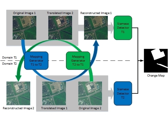
Activated by the problem formulation, the framework architecture is designed as shown in Figure 1. Our framework contains three main parts, namely, mapping generation, conditional discrimination, and Siamese detection. There are two mapping generators, two conditional discriminators, and two Siamese detectors. These six neural networks make up two paralleled streams: dual learning-based domain transfer and Siamese-based change decision. The two streams are discussed in detail in the following.

3.2.1. Domain Transfer Stream

Domain transfer for bi-temporal VHR optical remote sensing images is aimed at eliminating the domain differences including color distribution, texture characteristics, and contextual information between paired bi-temporal images, which are mainly caused by different times, illumination and atmospheric conditions, and imaging sensors. Concatenating Figure 1b to Figure 1a, domain transfer stream is achieved by two mapping generators and two conditional discriminators as illustrated in Figure 2.

It is noted that the two generators translate images from one domain to the other and together make up a closed loop, while the two discriminators distinguish translated images from original images in the unchanged regions in two domains, respectively. This adversarial learning will continuously improve the generators and the discriminators, and thereby boost the performance of the domain transfer stream.

Although the DLF is first designed for unpaired image-to-image translation, being applied to paired image-to-image domain transfer provides the correct direction of gradient descent when training models, thus, stabilizing and shortening the training process. In practice, the CDLF doubles the number of training datasets, but further enhances stability and increases the fault tolerance of this method for change detection.

3.2.2. Change Decision Stream

Change detection on paired images in the same domain is more accurate and efficient than that performed in two different domains. Concatenating Figure 1c to Figure 1a, change decision stream is achieved by two mapping generators and two Siamese detectors. Taking one pair of the original image and the translated image in the same domain as an example, the dataflow of the Siamese detector is illustrated in Figure 3.

Paired images are used as input of the same FCN, and two multichannel feature maps serve as the output. Thereafter, we compute the pixel-wise Euclidean distance between two feature maps and produce a change map that has the same width and height as the input images but has only one channel. By comparing the change map with the corresponding reference map, the FCN will be updated guided by the contrastive loss, and therefore boost the performance of the change decision stream.

3.3. Loss Function

We propose a new loss function comprised of four types of terms: (1) adversarial loss to match the information distribution between fake images and real ones in two domains respectively; (2) cross-consistency loss to represent the distance from translated images to original ones in two domains, respectively; (3) self-consistency loss to prevent two mapping generators from contradicting each other; (4) contrastive loss to bring similar pixels closer and push dissimilar pixels apart.

3.3.1. Adversarial Loss

As the basic loss function in GAN, adversarial loss is first proposed by Goodfellow et al. [48] and is set to fool conditional discriminators that do not distinguish translated images from original images. In this research, we apply two adversarial losses in two domains, respectively to facilitate transforming image domains but retaining intrinsic features as expressed in Equations (10) and (11).

$$\begin{array}{ll}{\mathcal{L}}_{GAN}\left(G_{1to2},D_2,T_1,T_2\right)& ={\mathbb{E}}_{I^{\left(T_2\right)}~pai{r}^{\left(T_2\right)}}\left[\log D_2\left(I^{\left(T_2\right)}\right)\right]\\ & +{\mathbb{E}}_{I^{\left(T_1\right)}~pai{r}^{\left(T_1\right)}}\left[\log \left(1-D_2\left(G_{1to2}\left(I^{\left(T_1\right)}\right)\right)\right)\right]\end{array}$$

(10)

$$\begin{array}{ll}{\mathcal{L}}_{GAN}\left(G_{2to1},D_1,T_2,T_1\right)& ={\mathbb{E}}_{I^{\left(T_1\right)}~pai{r}^{\left(T_1\right)}}\left[\log D_1\left(I^{\left(T_1\right)}\right)\right]\\ & +{\mathbb{E}}_{I^{\left(T_2\right)}~pai{r}^{\left(T_2\right)}}\left[\log \left(1-D_1\left(G_{2to1}\left(I^{\left(T_2\right)}\right)\right)\right)\right]\end{array}$$

(11)

where, $G_{1to2}$ and $G_{2to1}$ try to map the images to the other domain and make them appear similar to the real images in the other domain, while $D_1$ and $D_2$ try to distinguish between fake and real images in domain $T_1$ and $T_2$, respectively. Therefore, the generators aim to minimize these losses against the discriminators that aim to maximize them such as in $\underset{G_{1to2}}{\min }\underset{D_2}{\max }{\mathcal{L}}_{GAN}\left(G_{1to2},D_2,T_1,T_2\right)$ and $\underset{G_{2to1}}{\min }\underset{D_1}{\max }{\mathcal{L}}_{GAN}\left(G_{2to1},D_1,T_2,T_1\right)$.

3.3.2. Cross-Consistency Loss

Cross-consistency loss is derived from the LogSoftmax function in [49], which is a special type of cross entropy loss often used in semantic labeling with CNN or FCN. As interpreted in Section 3.1, in the unchanged regions, the paired real image is the reference map of the paired fake image. Therefore, we set two cross-consistency losses here to facilitate training two mapping generators with the L1 distance losses as expressed in Equations (12) and (13).

$${\mathcal{L}}_{cross}\left(G_{2to1},T_1\right)={\mathbb{E}}_{I^{\left(T_1\right)}~pai{r}^{\left(T_1\right)},I^{\left(T_2\right)}~pai{r}^{\left(T_2\right)}}[\Vert \left(1-C\right)\otimes \left(G_{2to1}\left(I^{\left(T_2\right)}\right)-I^{\left(T_1\right)}\right){\Vert }_1]$$

(12)

$${\mathcal{L}}_{cross}\left(G_{1to2},T_2\right)={\mathbb{E}}_{I^{\left(T_2\right)}~pai{r}^{\left(T_2\right)},I^{\left(T_1\right)}~pai{r}^{\left(T_1\right)}}[\Vert \left(1-C\right)\otimes \left(G_{1to2}\left(I^{\left(T_1\right)}\right)-I^{\left(T_2\right)}\right){\Vert }_1]$$

(13)

where, $\Vert ·{\Vert }_1$ is the L1 distance loss to strictly represent distance. Minimizing these losses makes the generators achieve good mapping between two domains.

3.3.3. Self-Consistency Loss

As a result of the powerful expression capacity of deep neural networks, the mappings between two domains are generally stochastic and not unique. To facilitate the adversarial losses and reduce the randomness of the mapping generators, here the self-consistency losses are set to guarantee that the mappings should bring images back to the original images as illustrated in Figure 2. Similar to the cycle-consistency losses in CycleGAN [44], the self-consistency losses in two domains are expressed in Equations (14) and (15).

$${\mathcal{L}}_{self}\left(G_{1to2},G_{2to1},T_1\right)={\mathbb{E}}_{I^{\left(T_1\right)}~pai{r}^{\left(T_1\right)}}[\Vert G_{2to1}\left(G_{1to2}\left(I^{\left(T_1\right)}\right)\right)-I^{\left(T_1\right)}{\Vert }_1]$$

(14)

$${\mathcal{L}}_{self}\left(G_{2to1},G_{1to2},T_2\right)={\mathbb{E}}_{I^{\left(T_2\right)}~pai{r}^{\left(T_2\right)}}[\Vert G_{1to2}\left(G_{2to1}\left(I^{\left(T_2\right)}\right)\right)-I^{\left(T_2\right)}{\Vert }_1]$$

(15)

where, $\Vert \cdot {\Vert }_1$ is the L1 distance loss. By minimizing these losses, it reduces the randomness of generators and provides a positive direction for the convergence procedure.

3.3.4. Contrastive Loss

FCSN plays an important role in ensuring effective decision making. It aims to make the feature points of unchanged pixel pairs closer to each other, and make the ones of changed pixel pairs considerably more distant in the output change map. In order to process the relationship between paired data in Siamese-based networks, Hadsell et al. [50] introduced a contrastive loss. In our proposed DLSF, the contrastive loses are set to evaluate whether the FCSN is trained well as expressed in Equations (16) and (17).

$${\mathcal{L}}_{con}\left(S_1,T_1\right)=mean\left({\mu }_U\left(1-C\right)\cdot p{D}^2\left(T_1\right)+{\mu }_{C}C\cdot max{\left(0,m-pD\left(T_1\right)\right)}^2\right)$$

(16)

$${\mathcal{L}}_{con}\left(S_2,T_2\right)=mean\left({\mu }_U\left(1-C\right)\cdot p{D}^2\left(T_2\right)+{\mu }_{C}C\cdot max{\left(0,m-pD\left(T_2\right)\right)}^2\right)$$

(17)

where, $m$ is a distance threshold which is set to be 2 here. ${\mu }_U$ and ${\mu }_C$ denote the relative importance for unchanged and changed pixel distribution, respectively, which are designed with global average frequency balancing, as shown in Equations (18) and (19).

$${\mu }_U=\frac{N\times W\times H}{{{\displaystyle \sum }}_{n=1}^{N}sum\left(1-C^{\left(n\right)}\right)}$$

(18)

$${\mu }_C=\frac{N\times W\times H}{{{\displaystyle \sum }}_{n=1}^{N}sum\left(C^{\left(n\right)}\right)}$$

(19)

where, $N$ is the total number of training sample pairs. $W$ and $H$ are the width and height of one image patch, respectively. $pD(\cdot )$ denotes the evaluation of pairwise Euclidean distance between two feature maps without changing the shape of the input image patches. As Equations (20) and (21) show, $pD\left(T_1\right)$ denotes the pixel-wise distance of two paired images in domain $T_1$, while $pD\left(T_2\right)$ denotes the distance of that in domain $T_2$.

$$pD{\left(T_1\right)}_{i,j}={\mathbb{E}}_{I^{\left(T_1\right)}~pai{r}^{\left(T_1\right)},I^{\left(T_2\right)}~pai{r}^{\left(T_2\right)}}[\Vert S_1{\left(G_{2to1}\left(I^{\left(T_2\right)}\right)\right)}_{i,j}-S_1{\left(I^{\left(T_1\right)}\right)}_{i,j}{\Vert }_2]$$

(20)

$$pD{\left(T_2\right)}_{i,j}={\mathbb{E}}_{I^{\left(T_2\right)}~pai{r}^{\left(T_2\right)},I^{\left(T_1\right)}~pai{r}^{\left(T_1\right)}}[\Vert S_2{\left(G_{1to2}\left(I^{\left(T_1\right)}\right)\right)}_{i,j}-S_2{\left(I^{\left(T_2\right)}\right)}_{i,j}{\Vert }_2]$$

(21)

where, $\Vert \cdot {\Vert }_2$ is the L2 distance loss. Specific to pixel-level, the contrastive losses are expressed as Equations (22) and (23).

$${\mathcal{L}}_{con}\left(S_1,T_1\right)=\frac{1}{W\times H}{\displaystyle \sum }_{i=1}^W{\displaystyle \sum }_{j=1}^H{\mu }_U\left(1-C_{i,j}\right)\cdot p{D}^2{\left(T_1\right)}_{i,j}+{\mu }_C{C}_{i,j}\cdot max{\left(0,m-pD{\left(T_1\right)}_{i,j}\right)}^2$$

(22)

$${\mathcal{L}}_{con}\left(S_2,T_2\right)=\frac{1}{W\times H}{\displaystyle \sum }_{i=1}^W{\displaystyle \sum }_{j=1}^H{\mu }_U\left(1-C_{i,j}\right)\cdot p{D}^2{\left(T_2\right)}_{i,j}+{\mu }_C{C}_{i,j}\cdot max{\left(0,m-pD{\left(T_2\right)}_{i,j}\right)}^2$$

(23)

In general, our full objective is an integration of the aforementioned loss functions, as expressed in Equation (24).

$$\begin{array}{ll}\mathcal{L}\left(G_{1to2},G_{2to1},D_1,D_2,S_1,S_2\right)& ={\lambda }_{GAN}\cdot \left[{\mathcal{L}}_{GAN}\left(G_{1to2},D_2,T_1,T_2\right)+{\mathcal{L}}_{GAN}\left(G_{2to1},D_1,T_2,T_1\right)\right]\\ & +{\lambda }_{cross}\cdot \left[{\mathcal{L}}_{cross}\left(G_{2to1},T_1\right)+{\mathcal{L}}_{cross}\left(G_{1to2},T_2\right)\right]\\ & +{\lambda }_{self}\cdot \left[{\mathcal{L}}_{self}\left(G_{1to2},G_{2to1},T_1\right)+{\mathcal{L}}_{self}\left(G_{2to1},G_{1to2},T_2\right)\right]\\ & +{\lambda }_{con}\cdot \left[{\mathcal{L}}_{con}\left(S_1,T_1\right)+{\mathcal{L}}_{con}\left(S_2,T_2\right)\right]\end{array}$$

(24)

where, $\lambda$ denotes the relative importance for each of these four loss functions. Therefore, our main solutions are expressed as Equations (25) and (26).

$$G_{1to2}^{*},G_{2to1}^{*},S_1^{*},S_2^{*}=arg\underset{G_{1to2},G_{2to1},S_1,S_2}{\min }\mathcal{L}\left(G_{1to2},G_{2to1},D_1,D_2,S_1,S_2\right)$$

(25)

$$D_1^{*},D_2^{*}=arg\underset{D_1,D_2}{\max }\mathcal{L}\left(G_{1to2},G_{2to1},D_1,D_2,S_1,S_2\right)$$

(26)

Guided by certain supervised references, we train all the networks on the same timeline. When predicting, however, only two trained mapping generators and two trained Siamese detectors are used for change detection.

3.4. Implementation

Since bi-temporal VHR optical remote sensing images are of large scale, in this paper, we make global normalizations in their own domains, respectively, and then crop them to small patches sized $256\times 256$ for later training and predicting. The training dataset is produced by randomly cutting from the original training areas. Certain overlapped and rotated samples enhance the training effect. When predicting, we first make predictions on all small patches and then splice them together into the entire prediction image.

3.4.1. Network Architecture

As illustrated in Figure 4, our two mapping generators are deep FCNs, and each one consists of two down-sampling convolutional blocks, nine residual blocks, and two up-sampling transposed convolutional blocks, which are followed by a convolutional layer and a linear activation function TanH. Unlike in the generators, only one down-sampling and up-sampling convolutional block is present in the conditional discriminators and Siamese detectors. The conditional discriminators comprise four convolutional blocks, followed by a discriminant transposed convolutional layer. The Siamese detectors compose seven convolutional blocks, followed by a transposed convolutional layer and a TanH activation.

Here, setting down-sampling and up-sampling blocks facilitates the networks learning of high-level features and enhances the generalization of mapping models in domain transfer. In order to prevent losing image information, no pooling layer is set in our neural networks. Instead, the down-sampling and up-sampling convolutional layers consist of convolution kernels sized $3\times 3$ with reflection padding 1 and stride 2, while the common convolutional layers consist of convolution kernels sized $3\times 3$ with reflection padding 1 and stride 1. The activation function in the blocks of generators is Rectified Linear Unit (ReLU), while the one in the blocks of discriminators and detectors is Leaky Rectified Linear Unit (Leaky ReLU) with a negative slope of 0.2. Instance normalization is used in all the blocks of these six networks. Remarkably, the first four convolutional blocks of the discriminator and the detector in the same domain share the same weights. In general, the memory occupations of these three types of neural networks are 11.378M, 0.964M and 1.973M, respectively.

3.4.2. Training Procedure

With our proposed DLSF, bi-temporal VHR remote sensing images are the direct inputs for the map generation without any pre- or post-processing. The two sets of translated images that serve as the outputs are recombined with the original images according to the domain. These sets of images are then regarded as the inputs of the conditional discriminations and Siamese detections. For forward propagation, we carry out generation, discrimination, and detection in sequence. Whereas, for backward propagation we update detectors, discriminators, and generators in the opposite order.

For all the experiments, we aim to obtain well trained models through the training procedure that mainly pursues to minimize the full objective $\mathcal{L}\left(G_{1to2},G_{2to1},D_1,D_2,S_1,S_2\right)$. According to the implementations in CycleGAN [44] and conditional pixel-to-pixel GAN [51], we set both ${\lambda }_{GAN}$ and ${\lambda }_{con}$ to be ${10}^{-2}$, set ${\lambda }_{self}$ to be ${10}^{-1}$, and set ${\lambda }_{cross}$ to be 1 in Equation (24). In order to stabilize the training procedures, we choose the least-squares loss specifically for ${\mathcal{L}}_{GAN}$ instead of the negative log likelihood loss in traditional GAN. For the six neural networks, all the weights and biases of the layers are first initialized with random values from zero-mean Gaussian distribution with a standard deviation of 0.1, and then optimized using Adaptive Moment Estimation (Adam) [52] solver when training.

Given the complexity of this framework, our optimization is designed to train all the networks in the same process. The detailed procedures of forward and backward propagations in one epoch are presented in

Table 2. The overview of the optimization sequence in one epoch.

Inputs:	Paired images in domain $T_1$: $I^{\left(T_1\right)}~pai{r}^{\left(T_1\right)}$ Paired images in domain $T_2$: $I^{\left(T_2\right)}~pai{r}^{\left(T_2\right)}$ Corresponding binary change map references: $C$
$for i\leftarrow 1 to N$
Forwards:	$I_i^{\left(T_1\right)}\to G_{1to2}\Rightarrow translated{I}_i^{\left(T_1\right)}\to G_{2to1}\Rightarrow reconstructed{I}_i^{\left(T_1\right)}$ $I_i^{\left(T_2\right)}\to G_{2to1}\Rightarrow translated{I}_i^{\left(T_2\right)}\to G_{1to2}\Rightarrow reconstructed{I}_i^{\left(T_2\right)}$ $I_i^{\left(T_1\right)},translated{I}_i^{\left(T_2\right)},C_i\to D_1$ $I_i^{\left(T_2\right)},translated{I}_i^{\left(T_1\right)},C_i\to D_2$ $I_i^{\left(T_1\right)},translated{I}_i^{\left(T_2\right)},C_i\to S_1$ $I_i^{\left(T_2\right)},translated{I}_i^{\left(T_1\right)},C_i\to S_2$
Backwards:	Update $S_1$ and $S_2$ with ${\mathcal{L}}_{con}\left(T_1\right)$ and ${\mathcal{L}}_{con}\left(T_2\right)$ Update $D_1$ and $D_2$ with ${\mathcal{L}}_{GAN}\left(G_{1to2},D_2,T_1,T_2\right)$ and ${\mathcal{L}}_{GAN}\left(G_{2to1},D_1,T_2,T_1\right)$ Update $G_{1to2}$ and $G_{2to1}$ with $\mathcal{L}\left(G_{1to2},G_{2to1},D_1,D_2,S_1,S_2\right)$
$end$
Outputs:	Well trained mapping generators: $G_{1to2}^{*}$ and $G_{2to1}^{*}$ Well trained Siamese detectors: $S_1^{*}$ and $S_2^{*}$

.

3.4.3. Predicting Detail

Although our proposed DLSF produces six well trained models after training, only two mapping generators and two Siamese detectors are used in predicting the test dataset. Similar to the training procedure, the generators, $G_{1to2}^{*}$ and $G_{2to1}^{*}$, are responsible for the transformation of the representations of paired images between two domains and production of two sets of patches as the inputs of the detectors afterward. Then Siamese detectors, $S_1^{*}$ and $S_2^{*}$, are mainly responsible for detecting the changed regions in two domains respectively, and they will produce two change probability maps in which the pixel values are between 0 and 1. At last, the final prediction result is achieved by the binarization of the mean value of these two change probability maps at the middle threshold of 0.5.

4. Experiments

4.1. Datasets Description

SZTAKI airchange benchmark: This benchmark dataset contains 12 bi-temporal VHR optical remote sensing image pairs and 12 corresponding change map references [26,53]. With over five years of differences, the image pairs are acquired at MTA SZTAKI, Budapest, Hungary. All the image sizes are $952\times 640$ with a resolution of 1.5 meter per pixel. The corresponding ground reference data are binary change maps drawn by hand for the following types of changes: (1) new built-up regions, (2) building operations, (3) planting of large group of trees, (4) fresh plough land, and (5) groundwork before building cover. Certain typical sample image pairs are illustrated in Figure 5. We take nine of the image pairs as the training samples, and the remaining three pairs as the testing samples. Therefore, the corresponding nine reference change maps were used for training procedure, while the corresponding three reference change maps were used for assessment.

Shenzhen dataset: This dataset contains two registered large scale bi-temporal VHR remote sensing images that cover approximately 182 square kilometers with the size of $5233\times 8677$ and $10466\times 17354$, respectively, which were acquired in the same district of Shenzhen, Guangzhou Province, China, but at different times. As shown in Figure 6, the image captured by SPOT 6 in 2014 has a resolution of 2 meter per pixel, while the image captured by GeoEye-1 in 2015 has a resolution of 1 meter per pixel. We classify the land cover of this dataset into the following six primary categories: (1) building group, (2) road and highway, (3) tree and vegetation, (4) cultivated land, (5) barren land, and (6) others. According to the classification rules above, we give the binary ground reference change maps by whether the regions at the same geographic location belong to different categories or not. We take three quarters of the area in paired images as the training areas, which leaves one quarter of the area as the testing areas. As compared with the SZTAKI dataset, the Shenzhen dataset covers a larger area of land surface and has more types of ground targets with a complex distribution.

4.2. Methods Comparison

In this research, the performance of the proposed DLSF is compared with that of several state-of-the-art conventional, machine learning-based and deep learning-based methods as follows:

• CVA [19]: Derived from the simple difference algorithm, CVA is a classic method for unsupervised change detection in remote sensing. By using a magnitude of difference vectors, CVA is able to achieve pixel-level change detection. In this competitive method, we use pixel-level change vectors to calculate the threshold by K-means clustering to achieve change detection.
• SVM [28]: As the most typical case of machine learning, SVM aims to make a generalized linear classification on dataset, and then find the decision boundary in high dimensional space. It is used for both supervised and unsupervised change detection. In this competitive method, we perform the experiments using a Gaussian radial basis function (RBF) kernel. And the SVM hyper-parameters are selected by a three-fold cross-validation.
• CNN [34]: This network is not only used for image classification, but also is applied to extract positive and meaningful features. By purposefully designing the network architecture and loss function, the features from the CNN process provide guidance for the supervised change detection.
• GAN [35]: With basic CNN network, GAN adds a discriminator for adversarial learning. In many image processing tasks, as compared with CNN, GAN has better generalization ability, and displays almost the same performance of CNN with fewer input training samples.
• DSCN [38]: Derived from the Siamese network, DSCN aims to extract robust features from two paired images with one CNN, which has no down- or up-sampling layers. With the convergence of contrastive loss, the model is able to detect the changed regions by calculating the pairwise Euclidean distance.
• SCCN [39]: As an extension of the Siamese network, SCCN is specifically designed for supervised change detection on heterogeneous remote sensing images. It maps two input images into the same feature space with a deep neural network comprised of one convolutional layer and several coupling layers, then it detects the changed regions by calculating the distance of paired images in the target feature space.

4.3. Evaluation Metrics

In order to prove the validity and effectiveness of our proposed DLSF for change detection, the following three indices are used to evaluate the accuracy of the final results.

Overall Accuracy (OA): The total accuracy is often used to assess the overall capacity of the change detection method, as expressed in Equation (27).

$$OA=\frac{TP+TN}{TP+TN+FP+FN}$$

(27)

where, $TP$ is the number of changed pixels correctly detected, $TN$ is the number of unchanged pixels correctly detected, $FP$ is the number of unchanged pixels incorrectly detected as changed, $FN$ is the number of changed pixels incorrectly detected as unchanged.

Kappa Coefficient (KC): This index is a statistical measure that reflects the consistency between experimental result and reference, as expressed in Equation (28).

$$\kappa =\frac{p_0-p_e}{1-p_e}$$

(28)

where, $p_0$ indicates the true consistency equaling $OA$ here and $p_e$ indicates the theoretical consistency, as expressed in Equation (29).

$$p_e=\frac{\left(TP+FP\right)\left(TP+FN\right)+\left(FN+TN\right)\left(FP+TN\right)}{{\left(TP+TN+FP+FN\right)}^2}$$

(29)

F1 Score (F1): This statistical magnitude is often used to evaluate neural network models and is calculated by precision rate and recall rate, as expressed in Equation (30).

$$F1=\frac{2\times \frac{TP}{TP+FP}\times \frac{TP}{TP+FN}}{\frac{TP}{TP+FP}+\frac{TP}{TP+FN}}=\frac{2TP}{2TP+FP+FN}$$

(30)

For the three evaluation indices, as the values of OA, KC, and F1 become larger, the change detection method is better.

4.4. Experimental Setup

We conduct two experiments on the aforementioned two datasets to verify the accuracy and efficiency of this method using certain training paired samples and testing paired samples with the ratio of approximately 3:1 as interpreted in Section 4.1. The size of all the paired samples and corresponding references is $256\times 256$, except for channel 3 and 1 respectively.

For the optimization procedure, we set 200 epochs to make the models converge and apply Adam solver with the batch size of 1. All the networks are trained from scratch with the learning rate of $2\times {10}^{-4}$. For the first 100 epochs, the learning rate is kept the same and is then linearly decayed to 0 for the next 100 epochs. The decay rates for the moment estimates are 0.9 and 0.999, respectively, and the epsilon is ${10}^{-8}$.

In the present research, the proposed DLSF are implemented in a PyTorch environment, which offers an effective programming interface written in Python. The experiments are performed on a computer with Intel Core i7, 16GB RAM and NVIDIA GTX1080 GPU. The time for one forward propagation and backward propagation on one sample patch pair is approximately 0.8 second, and the times for training one epoch on two datasets are approximately 495 and 790 seconds, respectively, for two datasets. With 200 epochs, the entire times for training the DLSF on SZTAKI benchmark and Shenzhen dataset are approximately 27 and 44 hours, respectively. On testing datasets, the time for one sample patch pair of size $256\times 256$ is just 0.25 second.

4.5. Results Presentation

The predicted binary change maps of our proposed DLSF and all the competitors on SZTAKI airchange benchmark and Shenzhen dataset are depicted in Figure 7 and Figure 8, respectively, where the black and white regions indicate the unchanged and changed regions.

As can be seen, since optical images have only three bands, the detection result of CVA contains numerous errors and noises. Specifically, substantial numbers of unchanged pixels are predicted as changed ones, while many changed regions are not detected or are detected as a couple of discrete regions. This result confirms that pixel-based methods does not consider the relationship of neighbor pixels, hence the prediction result will be not ideal. The SVM-based method gives better detection result than CVA does, as it incorporates contextual information as auxiliary data. Nevertheless, due to the weak generalization ability of the SVM model, the result of SVM is still unsatisfactory. With the embedding of deep learning technology, CNN learns certain implicit features and give better detection result as shown in Figure 7c and Figure 8c. With the same quantity of training samples, the convergence effect of GAN is not as good as that of CNN, but its prediction result on testing samples are better than those of CNN, as presented in Figure 7d and Figure 8d, which indicates that the GAN model is better for generalization in change detection. Notably, the results of DSCN and SCCN are largely free from noise, since they are designed specifically for change detection with consideration of the correlation of paired images and the contextual information of paired pixels. The outstanding performance of DSCN and SCCN indicates that the Siamese network-based methods are effective and robust for change detection tasks. As Figure 7g and Figure 8g show, our proposed DLSF, which integrates CDLF and FCSN, achieves the best detection result. As compared with the results of DSCN and SCCN, the contours of predicted changed regions by DLSF are more accurate and smoother, and there is hardly any negative influence from image noises.

With the change detection results of our proposed DLSF and other comparative methods, the evaluation metrics OA, KC, and F1 values for two datasets are computed and summarized in

Table 3. Overall accuracy, Kappa coefficients and F1 score over state-of-the-art methods on SZTAKI and Shenzhen datasets, and the size and processing rate of their models. The best values are in bold.

Dataset	Metric	CVA	SVM	CNN	GAN	DSCN	SCCN	Ours
SZTAKI	OA KC F1	0.6223 0.2705 0.4406	0.7569 0.4617 0.5830	0.8239 0.6501 0.6942	0.7914 0.6568 0.6935	0.8127 0.7516 0.7692	0.8396 0.7751 0.7970	0.8672 0.7905 0.8061
Shenzhen	OA KC F1	0.5109 0.2367 0.4054	0.7982 0.4855 0.5901	0.8350 0.6743 0.7214	0.8407 0.7356 0.7591	0.8263 0.7250 0.7394	0.8537 0.7541 0.7805	0.8986 0.7712 0.8149
Model size (megabyte) Rate (second/patch)		- 0.17	- 1.14	102.564 0.70	57.189 0.56	21.042 0.19	43.898 0.21	28.630 0.25

. As compared to CVA, SVM, CNN, GAN, DSCN, and SCCN, our proposed DLSF achieves the highest OA, KC, and F1 values of 0.8672, 0.7905, and 0.8066 on the SZTAKI benchmark, and of 0.8986, 0.7716, and 0.8149 on the Shenzhen dataset.

5. Discussion

Among the methods based on deep learning technology, we believe that the decisive factors are mainly the model architecture and the loss function. Therefore, in this section, discussion of these two factors will verify the uniqueness of our design.

5.1. Effect of Model Architectures

Deep neural networks have considerably diverse structures for different image processing tasks. The large and complex structures of the network have strong ability on feature representation and extraction, but they may induce data overfitting to some extent. On the contrary, small and simple network structures improve the generalization and efficiency of the models, but their limited expression may reduce the utilization of image information. Therefore, optimal model architectures best represent final performance. With regard to change detection in VHR optical remote sensing images, we design the models specifically adapting the training samples and goals using quantitative experiments. In this subsection, certain analyses on the three main parts of the DLSF are discussed.

5.1.1. Mapping Generator

With residual network as the baseline, we design this mapping generator that comprises two down-sampling layers, two up-sampling layers, and several residual blocks. On VHR optical remote sensing images, clear image details provide tremendous information and complicate change detection. Here the down- and up-sampling processes not only facilitate the networks learning high level features, but also reduce the negative impact from tiny ground targets in domain transfer, for example, layout of cars, seasonal variations in crown size, and minor landslides. We made several comparative experiments with diverse mapping generators and the same conditional discriminators and Siamese detectors. The generators are different at the times of down- and up-sampling processes and the number of residual blocks. The detection results on a typical paired sample are illustrated in Figure 9.

As Figure 9 shows, the mapping generators comprised of more residual blocks give better performances of change detection. With the same number of residual blocks, for the VHR remote sensing images with resolutions of 1 to 2 meters per pixel, two down- and up-sampling processes are able to filter out most tiny objects and noises. It is noteworthy that the mapping generators comprised of more than two down- and up-sampling processes will induce certain detection errors.

5.1.2. Conditional Discriminator

In conventional GAN, both global and patch-based discriminators pursue the same goal of processing real patches as binary maps with all pixel values of 1, and fake patches as binary maps with all pixel values of 0. The backward propagation for these types of discriminators activate generators to translate all the patch information from fake presentations to real ones. This process will transform the domain and revise the information of the original image, and then mislead the Siamese detector afterward. We conducted several experiments with diverse patch-based, global, and our conditional discriminators, and the results are illustrated in Figure 10.

It is noted that the global $256\times 256$ discriminator facilitates the generator producing far more realistic images than the $32\times 32$ patch-based discriminator. Nevertheless, all the conventional discriminators revised the original features and suppressed the differences of paired images simultaneously in the unchanged and changed regions, which induced pool detection results. Our proposed conditional discriminator is able to activate the generators to only translate the unchanged regions from fake presentation to a real one, without preserving the changed areas. As has been demonstrated, the adversarial learning with our proposed conditional discriminator is the most effective.

5.1.3. Siamese Detector

In terms of working mechanisms, FCSN has inputs, outputs, and architectures that are similar to the conditional discriminator, but requires additional network layers to recognize change regions. In an ideal situation, perfect discriminators in CDLF will process the unchanged regions of paired patches into the same value of 1, and therefore the pairwise Euclidean distances of paired pixels are close to 0. In contrast, the changed regions of paired patches will process to different random values, and therefore the pairwise Euclidean distances of paired pixels are greater than 0. At this point, we suggest that the weights of the conditional discriminator provide guidance to be shared in the first several layers of the Siamese detector. We conducted two experiments with two frameworks on Shenzhen dataset. The former framework separately trains discriminators and detectors, while the latter framework trains the weights shared discriminators and detectors. The change detection results are illustrated in Figure 11.

As Figure 11 shows, the third row gives the change detection results for training of the discriminators and detectors separately, while the fourth row gives the ones for the weights shared training of the discriminators and detectors. Both performances are almost the same, but the consumed times are different. For SZTAKI benchmark and Shenzhen dataset, the times for separate training are approximately 638 and 935 seconds per epoch, respectively, while that for weights shared training are approximately 495 and 790 seconds per epoch, respectively. It is noteworthy that the latter training way has earned nearly 145 seconds as compared with the former in every epoch.

5.2. Effect of Loss Functions

As the representative of training goal, loss function is the guidance for the convergence procedure of models. In order to verify the effectiveness and uniqueness of our loss functions, we conducted several comparative experiments on the SZTAKI and Shenzhen datasets with different losses. The training and testing OA with five different losses are computed and summarized in

Table 4. Training and testing overall accuracy on SZTAKI and Shenzhen dataset for different losses.

Dataset	SZTAKI		Shenzhen
OA	Training	Testing	Training	Testing
con GAN+con GAN+self+con GAN+cross+con GAN+cross+self+con	0.9536 0.9815 0.9673 0.9208 0.9140	0.8127 0.8256 0.8381 0.8605 0.8672	0.9650 0.9903 0.9724 0.9409 0.9377	0.8263 0.8421 0.8517 0.8850 0.8986

. In the following, we respectively make certain detailed interpretations on the effects of adversarial, cross-consistency, and self-consistency losses.

As can be seen, when the loss function becomes more complex, the training OAs on two datasets are gradually declining while the testing OAs are continuously growing. It is confirmed that complex loss functions have weaker fitting ability on training samples but have stronger generalization ability on testing samples.

Without adversarial loss, the feature extractor and decision maker are regarded as a simple Siamese network and a contrastive loss. As shown in the first and second rows in Table 4, with the addition of GAN, the training and testing OAs have significantly increased, which indicates that using one model to simultaneously detect unchanged and changed regions is difficult

For cross-consistency loss, we considered a rigorous study on the working mechanism of GAN. The goal of adversarial learning between generator and discriminator is to pursue the Nash equilibrium of these two networks. The convergence of objective in this adversarial learning indicates that the models have reached a mutually stable stage, but not the best ones. It is noteworthy that certain conventional deep learning models such as CNN and FCN perform the best classification and feature extraction due to the participation of references. Therefore, we set cross-consistency loss here to be a direct guidance facilitating adversarial loss to learn the best models. As shown in the third and fifth rows in Table 4, the overall accuracy of change detection on two datasets has prominently increased with the addition of cross-consistency.

As a technical trick, the self-consistency aims to reduce the randomness of mapping generators when training the DLSF. Without self-consistency loss, the CDLF is regarded as two “opposite” image-to-image translation models based on conditional pixel-to-pixel GAN [51]. As shown in the fourth and fifth rows in Figure 4, the addition of self-consistency has slightly improved the training and testing OAs on two datasets. Meanwhile during the training procedure, self-consistency enables the DLSF to rapidly achieve convergence.

6. Conclusions

In this paper, we propose a DLSF for change detection using bi-temporal VHR optical remote sensing images. With the proposed CDLF, we successfully reduced the domain differences between paired images, then suppressed the differences of unchanged regions and highlight the differences of changed regions. Meanwhile the proposed FCSN successfully detected the changes on bi-temporal images and achieved better detection results as compared with other state-of-the-art methods. Massive experiments on SZTAKI benchmark and Shenzhen dataset confirmed that our proposed method is advantageous with regard to fast processing velocity, small model size, and high accuracy.

Nevertheless, the proposed DLSF involves two major limitations. First, with the complex DLSF process, the training speed is slow, and the convergence curves are full of oscillations (see Appendix Figure A1 for more details). Second, in the early period of training, the updates on the two Siamese detectors are useless, because the CDLF has no ability to achieve the cross-domain translations at that time. In future studies, on the premise of ensuring detection accuracy, we plan to simplify the full objective and try to design an intelligent optimization strategy for training the models.

References

- Singh, A. Review article digital change detection techniques using remotely-sensed data. Int. J. Remote Sens. 1989, 10, 989–1003. [Google Scholar] [CrossRef]
- Lu, D.; Mausel, P.; Brondizio, E.; Moran, E. Change detection techniques. Int. J. Remote Sens. 2004, 25, 2365–2401. [Google Scholar] [CrossRef]
- Radke, R.J.; Andra, S.; Al-Kofahi, O.; Roysam, B. Image change detection algorithms: A systematic survey. IEEE Trans. Image Process. 2005, 14, 294–307. [Google Scholar] [CrossRef] [PubMed]
- Demir, B.; Bovolo, F.; Bruzzone, L. Updating land-cover maps by classification of image time series: A novel change-detection-driven transfer learning approach. IEEE Trans. Geosci. Remote Sens. 2013, 51, 300–312. [Google Scholar] [CrossRef]
- Jin, S.; Yang, L.; Danielson, P.; Homer, C.; Fry, J.; Xian, G. A comprehensive change detection method for updating the national land cover database to circa 2011. Remote Sens. Environ. 2014, 29, 78–92. [Google Scholar] [CrossRef]
- Kennedy, R.E.; Townsend, P.A.; Gross, J.E.; Cohen, W.B.; Bolstad, P.; Wang, Y.Q.; Adams, P.; Gross, J.E.; Goetz, S.J.; Cihlar, J. Remote sensing change detection tools for natural resource managers: Understanding concepts and tradeoffs in the design of landscape monitoring projects. Remote Sens. Environ. 2009, 113, 1382–1396. [Google Scholar] [CrossRef]
- Rokni, K.; Ahmad, A.; Selamat, A.; Hazini, S. Water feature extraction and change detection using multitemporal landsat imagery. Remote Sens. 2016, 6, 4173–4189. [Google Scholar] [CrossRef]
- Awad, M. Sea water chlorophyll a estimation using hyperspectral images and supervised artificial neural network. Ecol. Inform. 2014, 24, 60–68. [Google Scholar] [CrossRef]
- Singh, D.; Chamundeeswari, V.V.; Singh, K.; Wiesbeck, W. Monitoring and Change Detection of Natural Disaster (like Subsidence) Using Synthetic Aperture Radar (SAR) Data. In Proceedings of the International Conference on Recent Advances in Microwave Theory and Applications, Jaipur, India, 21–24 November 2008; pp. 419–421. [Google Scholar]
- Hu, T.; Huang, X.; Li, J.; Zhang, L. A novel co-training approach for urban land cover mapping with unclear landsat time series imagery. Remote Sens. Environ. 2018, 217, 144–157. [Google Scholar] [CrossRef]
- Ridd, M.K.; Liu, J. A comparison of four algorithms for change detection in an urban environment. Remote Sens. Environ. 1998, 63, 95–100. [Google Scholar] [CrossRef]
- Malmir, M.; Zarkesh, M.M.K.; Monavari, S.M.; Jozi, S.A.; Sharifi, E. Urban development change detection based on multi-temporal satellite images as a fast tracking approach-A case study of Ahwaz county, southwestern Iran. Environ. Monit. Assess. 2015, 187, 4295. [Google Scholar] [CrossRef]
- Bruzzone, L.; Bovolo, F. A novel framework for design of change-detection systems for very-high-resolution remote sensing images. Proc. IEEE 2013, 101, 609–630. [Google Scholar] [CrossRef]
- Bovolo, F.; Bruzzone, L. A detail-preserving scale-driven approach to change detection in multitemporal SAR images. IEEE Trans. Geosci. Remote Sens. 2005, 43, 2963–2972. [Google Scholar] [CrossRef]
- Inglada, J.; Mercier, G. A new statistical similarity measure for change detection in multitemporal SAR images and its extension to multiscale change analysis. IEEE Trans. Geosci. Remote Sens. 2007, 45, 1432–1445. [Google Scholar] [CrossRef]
- Kittler, J.; Illingworth, J. Minimum error thresholding. Pattern Recognit. 1986, 19, 41–47. [Google Scholar] [CrossRef]
- Yang, W.; Yang, X.; Yan, T.; Song, H.; Xia, G.S. Region-based change detection for polarimetric SAR images using Wishart mixture models. IEEE Trans. Geosci. Remote Sens. 2016, 54, 6746–6756. [Google Scholar] [CrossRef]
- Wu, C.; Du, B.; Zhang, L. Slow feature analysis for change detection in multispectral imagery. IEEE Trans. Geosci. Remote Sens. 2014, 52, 2858–2874. [Google Scholar] [CrossRef]
- Malila, W.A. Change Vector Analysis: An Approach for Detecting Forest Changes with Landsat. LARS Symposia 1980, 385. [Google Scholar]
- Bovolo, F.; Bruzzone, L. A theoretical framework for unsupervised change detection based on change vector analysis in the polar domain. IEEE Trans. Geosci. Remote Sens. 2007, 45, 218–236. [Google Scholar] [CrossRef]
- Liu, S.; Bruzzone, L.; Bovolo, F.; Du, P. A Novel Sequential spectral Change Vector Analysis for Representing and detecting Multiple Changes in Hyperspectral Images. In Proceedings of the IEEE Geoscience and Remote Sensing Symposium, Quebec City, QC, Canada, 13–18 July 2014; pp. 4656–4659. [Google Scholar]
- Nielsen, A.A.; Conradsen, K.; Simpson, J.J. Multivariate alteration detection (MAD) and MAF postprocessing in multispectral, bitemporal image data: New approaches to change detection studies. Remote Sens. Environ. 1998, 64, 1–19. [Google Scholar] [CrossRef]
- Nielsen, A.A. The regularized iteratively reweighted MAD method for change detection in multi-and hyperspectral data. IEEE Trans. Image Process. 2007, 16, 463–478. [Google Scholar] [CrossRef]
- Feng, W.; Sui, H.; Tu, J.; Huang, W.; Sun, K. A novel change detection approach based on visual saliency and random forest from multi-temporal high-resolution remote-sensing images. Int. J. Remote Sens. 2018, 39, 7998–8021. [Google Scholar] [CrossRef]
- Bueno, I.T.; Junior, F.W.A.; Silveira, E.M.O.; Mello, J.M.; Carvalho, L.M.T.; Gomide, L.R.; Withey, K.; Scolforo, J.R.S. Object-based change detection in the Cerrado biome using landsat time series. Remote Sens. 2019, 11, 570. [Google Scholar] [CrossRef]
- Benedek, C.; Sziranyi, T. Change detection in optical aerial images by a multilayer conditional mixed Markov model. IEEE Trans. Geosci. Remote Sens. 2009, 47, 3416–3430. [Google Scholar] [CrossRef]
- Moser, G.; Angiati, E.; Serpico, S.B. Multiscale unsupervised change detection by Markov random fields and wavelet transforms. IEEE Geosci. Remote Sens. Lett. 2011, 8, 725–729. [Google Scholar] [CrossRef]
- Volpi, M.; Tuia, D.; Bovolo, F.; Kanevski, M.; Bruzzone, L. Supervised change detection in VHR images using contextual information and support vector machines. Int. J. Appl. Earth Obs. Geoinform. 2013, 20, 70–85. [Google Scholar] [CrossRef]
- Deng, J.; Wang, K.; Deng, Y.; Qi, G. PCA-based land-use change detection and analysis using multitemporal and multisensor satellite data. Int. J. Remote Sens. 2008, 29, 4823–4838. [Google Scholar] [CrossRef]
- Wang, X.; Liu, S.; Du, P.; Liang, H.; Xia, J.; Li, Y. Object-based change detection in urban areas from high spatial resolution images based on multiple features and ensemble learning. Remote Sens. 2018, 10, 276. [Google Scholar] [CrossRef]
- Tan, K.; Zhang, Y.; Wang, X.; Chen, Y. Object-based change detection using multiple classifiers and multi-scale uncertainty analysis. Remote Sens. 2019, 11, 359. [Google Scholar] [CrossRef]
- Lyu, H.; Lu, H.; Mou, L. Learning a transferable change rule from a recurrent neural network for land cover change detection. Remote Sens. 2016, 8, 506. [Google Scholar] [CrossRef]
- Gong, M.; Zhao, J.; Liu, J.; Miao, Q.; Jiao, L. Change detection in synthetic aperture radar images based on deep belief networks. IEEE Trans. Neural Netw. Learn. Syst. 2016, 27, 125–138. [Google Scholar] [CrossRef] [PubMed]
- Wang, Q.; Yuan, Z.; Du, Q.; Li, X. GETNET: A general end-to-end 2-D CNN framework for hyperspectral image change detection. IEEE Trans. Geosci. Remote Sens. 2019, 57, 3–13. [Google Scholar] [CrossRef]
- Gong, M.; Niu, X.; Zhang, P.; Li, Z. Generative adversarial networks for change detection in multispectral imagery. IEEE Geosci. Remote Sens. Lett. 2017, 14, 2310–2314. [Google Scholar] [CrossRef]
- Gong, M.; Yang, Y.; Zhan, T.; Niu, X.; Li, S. A generative discriminatory classified network for change detection in multispectral imagery. IEEE J. Sel. Top. Appl. Earth Observ. Remote Sens. 2019, 12, 321–333. [Google Scholar] [CrossRef]
- Niu, X.; Gong, M.; Zhan, T.; Yang, Y. A conditional adversarial network for change detection in heterogeneous images. IEEE Geosci. Remote Sens. Lett. 2019, 16, 45–49. [Google Scholar] [CrossRef]
- Zhan, Y.; Fu, K.; Yan, M.; Sun, X.; Wang, H.; Qiu, X. Change detection based on deep Siamese convolutional network for optical aerial images. IEEE Geosci. Remote Sens. Lett. 2017, 14, 1845–1849. [Google Scholar] [CrossRef]
- Liu, J.; Gong, M.; Qin, K.; Zhang, P. A deep convolutional coupling network for change detection based on heterogeneous optical and radar images. IEEE Trans. Neural Netw. Learn. Syst. 2018, 29, 545–559. [Google Scholar] [CrossRef]
- Yu, L.; Xie, J.; Chen, S.; Zhu, L. Generating labeled samples for hyperspectral image classification using correlation of spectral bands. Front. Comput. Sci. 2016, 10, 292–301. [Google Scholar] [CrossRef]
- Xia, Y.; He, D.; Qin, T.; Wang, L.; Yu, N.; Liu, T.; Ma, W. Dual Learning for Machine Translation. arXiv 2016, arXiv:1611.00179. [Google Scholar]
- Yi, Z.; Zhang, H.; Tan, P.; Gong, M. DualGAN: Unsupervised Dual Learning for Image-to-Image Translation. In Proceedings of the IEEE International Conference on Computer Vision (ICCV), Venice, Italy, 22–29 October 2017; pp. 2849–2857. [Google Scholar]
- Kim, T.; Cha, M.; Kim, H.; Lee, J.; Kim, J. Learning to Discover Cross-Domain Relations with Generative Adversarial Networks. In Proceedings of the 34th International Conference on Machine Learn. (ICML), Sydney, Australia, 6–11 August 2017; pp. 1857–1865. [Google Scholar]
- Zhu, J.; Park, T.; Isola, P.; Efros, A. Unpaired Image-to-Image Translation Using Cycle-Consistent Adversarial Networks. In Proceedings of the IEEE International Conference on Computer Vision (ICCV), Venice, Italy, 22–29 October 2017; pp. 2223–2232. [Google Scholar]
- Bertinetto, L.; Valmadre, J.; Henriques, J.; Vedaldi, A.; Torr, P. Fully-Convolutional Siamese Networks for Object Tracking. In Proceedings of the European Conference on Computer Vision (ECCV). Amsterdam, The Netherlands, 8–16 October 2016; pp. 850–865. [Google Scholar]
- Daudt, R.C.; Saux, B.L.; Buolch, A.; Gousseau, Y. Urban change Detection for Multispectral Earth Observation Using Convolutional Neural Networks. In Proceedings of the IEEE International Geoscience and Remote Sensing Symposium, Valencia, Spain, 22–27 July 2018; pp. 22–27. [Google Scholar]
- Daudt, R.C.; Saux, B.L.; Buolch, A. Fully Convolutional Siamese Network for Change Detection. arXiv 2018, arXiv:1810.08462. [Google Scholar]
- Goodfellow, I.J.; Pouget-Abadie, J.; Mirza, M.; Xu, B.; Warde-Farley, D.; Ozair, S.; Courville, A.; Bengio, Y. Generative Adversarial Nets. In Proceedings of the International Conference Neural Information Processing Systems (NIPS), Montreal, QC, Canada, 8–13 December 2014. [Google Scholar]
- Long, J.; Shelhamer, E.; Darrell, T. Fully Convolutional Network for Semantic Segmentation. IEEE Trans. Pattern Anal. Mach. Intell. 2017, 39, 640–651. [Google Scholar]
- Hadsell, R.; Chopra, S.; LeCun, Y. Dimensionality Reduction by Learning an Invariant Mapping. In Proceedings of the IEEE Computer Society Conference on Computer Vision and Pattern Recognition (CVPR), New York, NY, USA, 17–22 June 2006; 100. [Google Scholar]
- Isola, P.; Zhu, J.; Zhou, T.; Efros, A.A. Image-to-Image Translation with Conditional Adversarial Networks. In Proceedings of the Computer Vision and Pattern Recognition (CVPR), Honolulu, HI, USA, 21–26 July 2017; p. 632. [Google Scholar]
- Kimgma, D.P.; Ba, J.L. Adam: A Method for Stochastic Optimization. In Proceedings of the International Conference on Learning Representations, San Diego, CA, USA, 7–9 May 2015; pp. 1–13. [Google Scholar]
- Benedek, C.; Sziranyi, T. A mixed Markov model for change detection in aerial photos with large time differences. Int. Conf. Pattern Recognit. 2008, 12, 8–11. [Google Scholar]
Figure 1.
Framework of the proposed method for change detection using bi-temporal very-high-resolution (VHR) optical remote sensing images: (a) mapping generation, (b) conditional discrimination, (c) Siamese detection, (a)+(b) domain transfer stream, (a)+(c) change decision stream.
Figure 2.
Dataflow of the domain transfer stream. The values of white and black pixels are 1 and 0, and the values of gray pixels are random between 0 and 1.
Figure 3.
Dataflow of the Siamese detector. The changed pixels are white, while the unchanged pixels are black.
Figure 4.
Architectures of mapping generator, conditional discriminator, and Siamese detector.
Figure 5.
Sample image pairs and the corresponding change map references of SZTAKI benchmark: (a) images acquired at time , (b) Images acquired at time , (c) reference map.
Figure 6.
The overview of Shenzhen dataset and the corresponding change map reference: (a) image acquired at time , (b) image acquired at time , (c) reference map.
Figure 7.
The change detection results of comparative methods for the 3 test image pairs of the SZTAKI benchmark shown in Figure 5: (a) CVA, (b) SVM, (c) CNN, (d) GAN, (e) DSCN, (f) SCCN, (g) our DLSF, (h) reference map.
Figure 8.
The change detection results of comparative methods on the test area of Shenzhen dataset: (a) CVA, (b) SVM, (c) CNN, (d) GAN, (e) DSCN, (f) SCCN, (g) our DLSF, (h) reference map.
Figure 9.
The representative change detection results affected by generators with diverse structures: (a) one down- and up-sampling layer, (b) two down- and up-sampling layers, (c) three down- and up-sampling layers.
Figure 10.
The representative domain transfer results affected by diverse discriminators: (a) the fake image translated from domain to , (b) the fake image translated from domain to , (c) change detection results.
Figure 11.
The representative change detection results affected by diverse detectors: (a) image 1, (b) image 2, (c) the changes detected by separate training, (d) the changes detected by weights shared training, (e) reference map.