Establishment of a Real-Time Local Tropospheric Fusion Model

Abstract

The tropospheric delay is one major error source affecting the precise positioning provided by the global navigation satellite system (GNSS). This error occurs because the GNSS signals are refracted while travelling through the troposphere layer. Nowadays, various types of model can produce the tropospheric delay. Among them, the globally distributed GNSS permanent stations can resolve the tropospheric delay with the highest accuracy and the best continuity. Meteorological models, such as the Saastamoinen model, provide formulae to calculate temperature, pressure, water vapor pressure and subsequently the tropospheric delay. Some grid-based empirical tropospheric delay models directly provide tropospheric parameters at a global scale and in real time without any auxiliary information. However, the spatial resolution of the GNSS tropospheric delay is not sufficient, and the accuracy of the meteorological and empirical models is relatively poor. With the rapid development of satellite navigation systems around the globe, the demand for real-time high-precision GNSS positioning services has been growing dramatically, requiring real-time and high-accuracy troposphere models as a critical prerequisite. Therefore, this paper proposes a multi-source real-time local tropospheric delay model that uses polynomial fitting of ground-based GNSS observations, meteorological data, and empirical GPT2w models. The results show that the accuracy in the zenith tropospheric delay (ZTD) of the proposed tropospheric delay model has been verified with a RMS (root mean square) of 1.48 cm in active troposphere conditions, and 1.45 cm in stable troposphere conditions, which is significantly better than the conventional tropospheric GPT2w and Saastamoinen models.

1. Introduction

The troposphere is an important part of the Earth’s space environment and exerts an important control to the functioning of the global navigation satellite system (GNSS) technology. Tropospheric delay is one of the main error sources in GNSS precise positioning, as the GNSS signal is refracted while travelling through the troposphere. Generally, the tropospheric delay is estimated as a parameter during GNSS data processing. With the increasing demand for GNSS real-time applications, high-precision tropospheric delay augmentation information is essential to enhance convergence speed and precision of positioning [1].

At present, troposphere models are often used for tropospheric corrections in the GNSS, including the interferometric synthetic aperture radar (InSAR), and Very long baseline interferometry (VLBI). Local tropospheric models also significantly affect the performance of the differential global positioning system (DGPS), and the real time kinematic (RTK) and network RTK positioning systems [2,3,4]. With the increasing number of GNSS users, high-precision and stable positioning services in real time are expected. Meanwhile, the requirements in terms of accuracy for real-time troposphere models are also increasing. In order to address the issue, three types of real-time model of the troposphere are commonly used: the first type comprises empirical models of tropospheric key parameters, by which the tropospheric delay can be calculated without any additional information; the second type includes the traditional models based on meteorological data observed from the ground; the third type comprises the models established by the GNSS CORS (continuous operational reference system) networks.

The empirical model of tropospheric key parameters is used to derive the tropospheric delay directly by using only the model parameters, i.e., without any auxiliary information. Initially, the UNB (University of New Brunswick) series model was first established by Collins and Langley [5,6] for application to the US-wide area augmented navigation system. In North America, the UNB-estimated zenith tropospheric delay (ZTD) has a mean error of approximately 2 cm. The EGNOS (European Geostationary Navigation Overlay Service) model [7], simplified from the UNB3 model, has been used in European and Japanese satellite navigation augmentation systems [8,9]. Boehm established a global pressure and temperature (GPT) model using the Numerical Weather Model (NWM) product ERA-40 provided by the European Center for Medium-Range Weather Forecast (ECMWF) [10], which has been widely used in practice [11,12]. Lu C et al. developed an NWM-constrained Precise Point Positioning (PPP) processing system, in which tropospheric delay parameters derived from the ECMWF analysis were applied to multi-GNSS precise positioning [13]. Within this experiment, the convergence time was shortened, and the positioning accuracy also benefited from the NWM-constrained PPP solution. Lagler et al. improved and optimized some of the deficiencies of the GPT model and built a new empirical model (GPT2) [14]. Based on the GPT2 model, Boehm et al. extended the parameters to establish the Global Pressure and Temperature 2 wet (GPT2w) model [15]. The average accuracy of the estimated zenith wet delay (ZWD) from the GPT2w model is approximately 3.6 cm.

The second type of model, which estimates the tropospheric delay based on observed meteorological parameters, includes traditional models such as the Hopfield model [16], the Saastamoinen model [17], and the Black model [18]. These models estimate the tropospheric delay using meteorological data recorded by meteorological stations on the ground. The accuracy of the ZTD correction is usually in the decimeter range for these models, but can improve down to the centimeter range when the conditions are good. The accuracy of the correction obtained through the Hopfield model is related to the elevation. When the station is located at high elevation, the accuracy of the correction is noticeably decreased. On the other hand, the accuracy of the Saastamoinen model is less affected by elevation [19].

The third type of tropospheric delay models is GNSS-based, as the ZTD is calculated using GNSS observation data, based on which the model is built. Tao estimated the tropospheric ZWD using JPL (Jet Propulsion Laboratory) real-time orbital information, clock products, and PPP techniques, reaching an accuracy as low as 13 mm [20]. Ye et al. pointed out the feasibility of using PPP techniques to estimate accurate tropospheric delay [21]. Wang et al. estimated the tropospheric delay using CNES (Center National d’Etudes Spatiales)’s real-time corrections in near-real-time PPP, with a 6.5 mm deviation from the post-processing results, and with an RMS of 13 mm [22]. Shi et al. introduced a strategy entailing the modeling of ZWD estimates inside a real-time GNSS reference network with the aid of optimal fitting coefficients (OFCS) [23]. Dousa et al. exploited the PPP method using Kalman filtering and backward smoothing and developed a new strategy for a synchronous generation of real-time (RT) and near real-time (NRT) tropospheric products [24]. The strategy can be optimized for the latency or accuracy of NRT production. Dousa et al. developed a new concept for providing tropospheric augmentation corrections, by which a two-stage correction model is used to combine data from a Numerical Weather Model (NWM) and precise ZTDs estimated from GNSS permanent stations in regional networks [25]. In this way, the accuracy of ZTD estimates is improved by a factor of 2.5 or higher.

Moving from the first to the second and third model types, the modeling cost (time, manpower, and material resources) gradually increases, but the accuracy of the tropospheric delay model also increases.

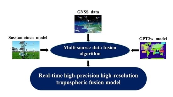
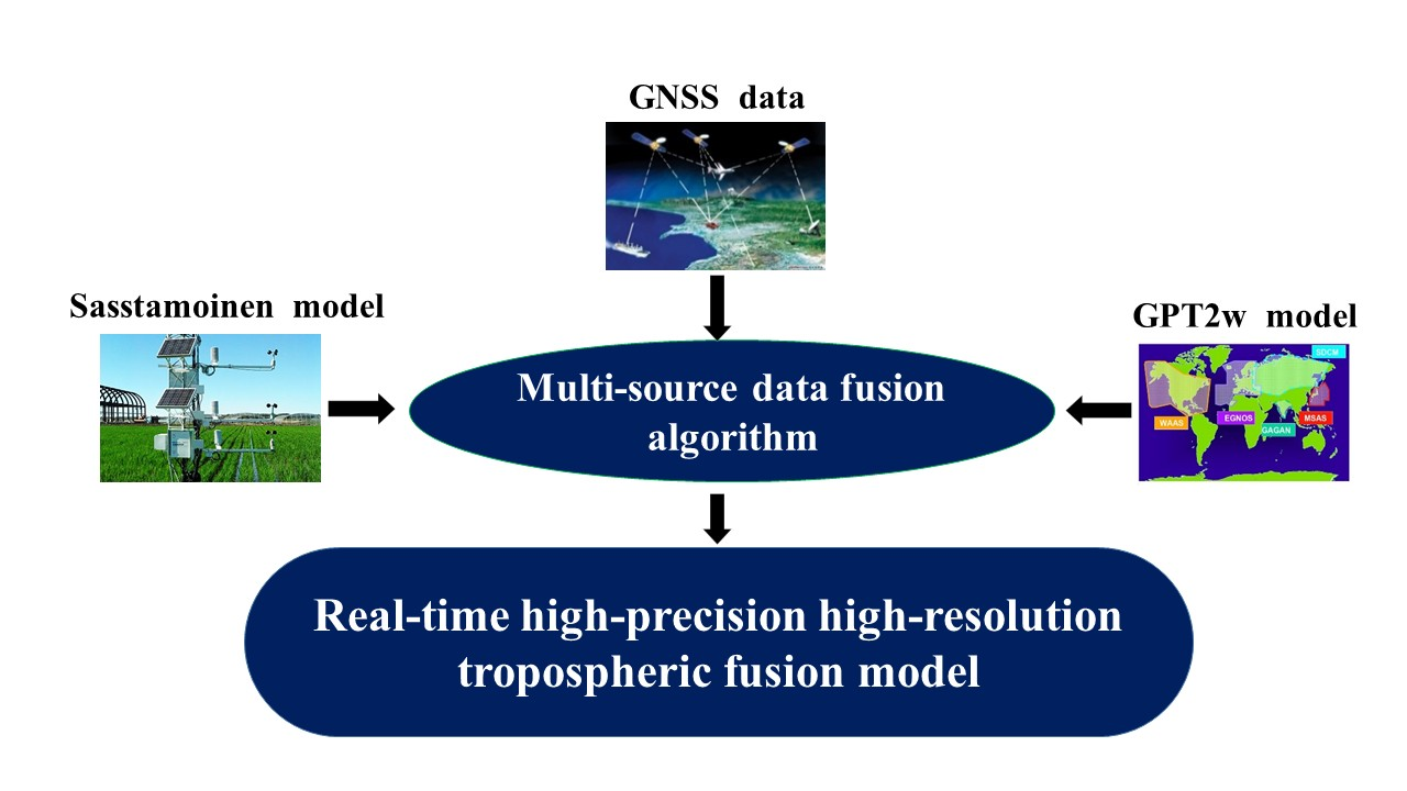
At present, GNSS CORS networks have been established in many regions of the world. In addition, meteorological observation networks are available in most areas. It is necessary to make full use of all the available observations to establish a better tropospheric fusion model. Therefore, this paper generates a real-time tropospheric fusion model using GNSS observation data, meteorological data, and a GPT2w empirical model, and validates it taking Hong Kong as a case study. The differences in terms of accuracy, and the systematic bias of different types of data are also discussed, and the Helmert variance component estimation is used to determine the precise weights of different observations. The systematic bias between different models was seen to be constant in each model epoch, and was quantified by least squares. The results of ZTDs estimates from multi-source data are compared with those obtained by GNSS processing.

Subsequently, we describe the overall strategy employed and the data used. The assessment and outcomes of the strategies adopted are then discussed, while considerations are presented in the conclusion.

2. Materials and Methods

2.1. Multisource Tropospheric Data

2.1.1. Zenith Tropospheric Delay Obtained by GNSS Processing

Currently, a large number of GNSS CORS networks have been established in China and around the world. High-precision tropospheric delay models can be obtained taking advantage of the real-time observation data of the GNSS CORS network. The methods for estimating the tropospheric delay using GNSS observations can be classified into two main types: the zero-difference mode and the double-difference mode.

In the zero-difference mode: the absolute tropospheric delay parameters are obtained using precision point positioning (PPP) techniques. The equation defining the error is as follows:

$$v_p^j(i)=\rho (i)+c\cdot \delta t(i)+c\cdot \delta t(j)+\delta {\rho }_{zd}(i)\cdot M({\theta }^i(i))-P^j(i)+{\epsilon }_p$$

(1)

$$v_{\mathsf{\Phi }}^j(i)=\rho (i)+c\cdot \delta t(i)+c\cdot \delta t(j)+\delta {\rho }_{zd}(i)\cdot M({\theta }^i(i))-\lambda \cdot N^j(i)-\lambda \cdot {\mathsf{\Phi }}^j(i)+{\epsilon }_{\mathsf{\Phi }}$$

(2)

where v is the observation correction, $j$ is the satellite number, $i$ is the corresponding observation epoch, c is the speed of light in the vacuum, $\delta t(i)$ is the receiver clock correction, $\delta t(j)$ is the satellite clock correction, $\delta {\rho }_{\mathrm{zd}}(i)$, $\mathrm{M}({\theta }^i(i))$ are the zenith troposphere delay and the corresponding projection function, ${\theta }^j(i)$ is the elevation angle of the satellite j, ${\epsilon }_p,{\epsilon }_{\mathsf{\Phi }}$ quantify the multipath, observation noise, and other unmodeled errors, $P_{(i)}^j,{\mathsf{\Phi }}_{(i)}^j$ are the corresponding combined observations with the ionospheric effects eliminated, $\lambda$ is the wave length, $\rho (i)$ is the geometric distance between the satellite and the receiver, and $N_{(i)}^j$ are the ambiguity parameters with ionospheric effects eliminated. Based on Equations (1) and (2), the total zenith troposphere delay of the station can be obtained by means of the Kalman filter.

Previous GNSS real-time applications have been implemented using the double-differential method. However, in order to obtain a stable tropospheric estimate, a new participating station needs to be introduced from 500 km away [26], which is not a convenient choice when the regional GNSS continuous operation reference network is utilized. Furthermore, zero-differential algorithms can provide accurate tropospheric estimates by taking advantage of the PPP technology without introducing stations located outside the network. The server receives the real-time orbital clock correction products from the IGS RTS (International GNSS Service Real Time Service) and calculates the tropospheric delay (GNSS-ZTD) for each GNSS station in real time in combination with the GNSS observations from the regional crustal movement observation network and the CORS stations. Using CORS observations, Shi et al. introduced a strategy for presenting regional atmospheric augmentation results with local troposphere corrections [23].

2.1.2. Zenith Tropospheric Delay Obtained by the Saastamoinen Model

Tropospheric delay models based on observed meteorological parameters such as the Hopfield model, the Saastamoinen model, the Ifadis model [27], and the AN model [28] can provide the zenith troposphere delay for the fusion model.

In the meteorological tropospheric models, the ZTD is obtained using meteorological parameters. The ZHD and ZWD are usually calculated separately. Saastamoinen proposed a tropospheric delay model based on meteorological parameters so that the ZTD can be calculated using the station latitude, altitude, temperature, pressure, and water vapor pressure [17]. The formula for the Saastamoinen model is as follows:

$$ZTD=ZHD+ZWD=\frac{0.0022768}{1-0.00266\cos (2\phi )-0.00000028H}(P+(\frac{1255}{T}+0.05)e)$$

(3)

where P (hPa) is the pressure, T (K) is the absolute temperature, e (hPa) is the water vapor pressure, ψ is the latitude, and H is the elevation of the station.

At present, there is a sufficient number of surface meteorological stations around the world to obtain real-time surface meteorological parameters (i.e., temperature, pressure, and water vapor pressure). Moreover, these devices are inexpensive. It is of great significance to correct tropospheric errors by taking full advantage of the surface meteorological parameters.

2.1.3. Zenith Tropospheric Delay Obtained by the GPT2w Model

The empirical models of tropospheric key parameters, such as the UNB series model, the EGNOS model, the TropGrid model and the GPT series models can also provide the zenith troposphere delay for the fusion model.

The aim of an empirical tropospheric delay model is to solve the problem of obtaining high-precision tropospheric delay without any auxiliary information. The GPT2w model is an advanced empirical troposphere model that uses meteorological data from the European Center for Medium Range Weather Forecast (ECMWF), whose published parameters include temperature, pressure, temperature lapse rate, water vapor pressure, mapping function coefficient, atmospheric weighted average temperature, and water vapor decrease factor decline rate. The model considers the annual and semiannual periods of the tropospheric parameters, and its governing expression is reported as Equation (4) below. The GPT2w parameters are expressed in global grids with a spatial resolution of 5 ° × 5 ° and 1 ° × 1 °. The globe is divided according to the grid, and the coefficient at each grid point is calculated. The parameter estimation of four grid points around the target station is calculated and then interpolated to the target position using a bilinear interpolation. The Saastamoinen model is used for the calculation of the ZHD in the GPT2w model using Equation (3), while the AN model (Askne and Nordius, 1987) is utilized to calculate the ZWD. The equations for the calculations are reported in Equations (5) and (6). The GPT2w model, thanks to its empirical nature, can provide empirical values of ZTD at any time and location, which are thus available as background fields for data fusion studies.

$$a=a_0+A_1\cos (\frac{doy}{365.25}2\pi )+B_1\sin (\frac{doy}{365.25}2\pi )+A_2\cos (\frac{doy}{365.25}4\pi )+B_2\sin (\frac{doy}{365.25}4\pi )$$

(4)

$$ZWD={10}^{-6}(k_2^{\prime }+\frac{k_3}{T_m})\frac{R}{(\beta +1)g_m}{e}_s$$

(5)

$$\frac{e}{e_0}={(\frac{P}{P_0})}^{\beta +1}$$

(6)

In Equation (4), a is the tropospheric key parameter to be sought, a₀ is the mean value, A₁ and B₁ are the annual cycle amplitudes, A₂ and B₂ are the semi-annual cycle amplitudes, doy is the day of the year. In Equation (5), $k_2^{\prime }$ and k₃ are the atmospheric refractive index constants provided by Thayer [29], where $k_2^{\prime }$= 16.529 k·mb⁻¹ and k₃ = 3.776 × 10⁵ k·mb⁻¹. Furthermore, T_m is the atmospheric weighted average temperature, g_m is the gravity acceleration, R_d is the gas ratio of dry air constant values 287.058 J·kg⁻¹·K⁻¹, e_s is the vapor pressure, β is calculated by Equation (6). The β parameter is one of the weather parameters provided by GPT2w, whose solution requires the fitting of meteorological profile data at the station.

2.2. Methods for Establishing the Local Tropospheric Fusion Model

2.2.1. Tropospheric Fusion Modeling

By fitting the ZTD values obtained by different means of observation using the appropriate model, a real-time local tropospheric fusion model can be developed. This paper proposes a method for determining the fitting coefficients for local troposphere modeling. The general form of the second-order fitting model consists of the following error equations:

ZTD_i,j,k are the ZTD observations at the station. The parameters to be solved are the ten fitting model coefficients, the Saastamoinen systematic bias, and the GPT2w systematic bias. The usual practice is to consider the systematic biases as model unknowns, and to estimate them together with the tropospheric fusion model coefficients using a least squares approach.

$$\left[\begin{array}{c}{v}^{GNSSi}\\ v^{SAASj}\\ v^{GPT2wk}\end{array}\right]=\left[\begin{array}{cccccccccccc}1& B_i& L_i& h_i& B_i{L}_i& B_i{h}_i& L_i{h}_i& B_i^2& L_i^2& h_i^2& 0& 0\\ 1& B_j& L_j& h_j& B_j{L}_j& B_j{h}_j& L_j{h}_j& B_j^2& L_j^2& h_j^2& 1& 0\\ 1& B_k& L_k& h_k& B_k{L}_k& B_k{h}_k& L_k{h}_k& B_k^2& L_k^2& h_k^2& 0& 1\end{array}\right]\left[\begin{array}{c}{a}_0\\ a_1\\ a_2\\ a_3\\ a_4\\ a_5\\ a_6\\ a_7\\ a_8\\ a_9\\ {\delta }_S\\ {\delta }_G\end{array}\right]+\left[\begin{array}{c}{\epsilon }_{GNSS}\\ {\epsilon }_{SAAS}\\ {\epsilon }_{GPT2w}\end{array}\right],Q_{ZTD}$$

(7)

$$v=ZT{D}_{fusion}-ZT{D}_{i,j,k}-ZT{D}_0$$

(8)

where the subscripts i,j,k denote the indexes of the reference GNSS stations, meteorological stations, and grid points, respectively, (B, L) are the latitude and longitude of the observation station, and h is the ellipsoid height. The ten fitting coefficients are represented by a₀, a₁,……a₉; δ_S is the systematic bias between the Saastamoinen model and the fusion model, and δ_G is the systematic bias between the GPT2w model and the fusion model. We assume that there is no systematic bias between the GNSS-based model and the fusion model.

The form of the tropospheric delay model is not fixed. For alternative forms, the reader can refer to the adaptive model proposed by Shi [23]. In this paper, the adaptive model has been tested, and it has been found suitable for the research. If an even better precision is needed, the adaptive model can be adopted.

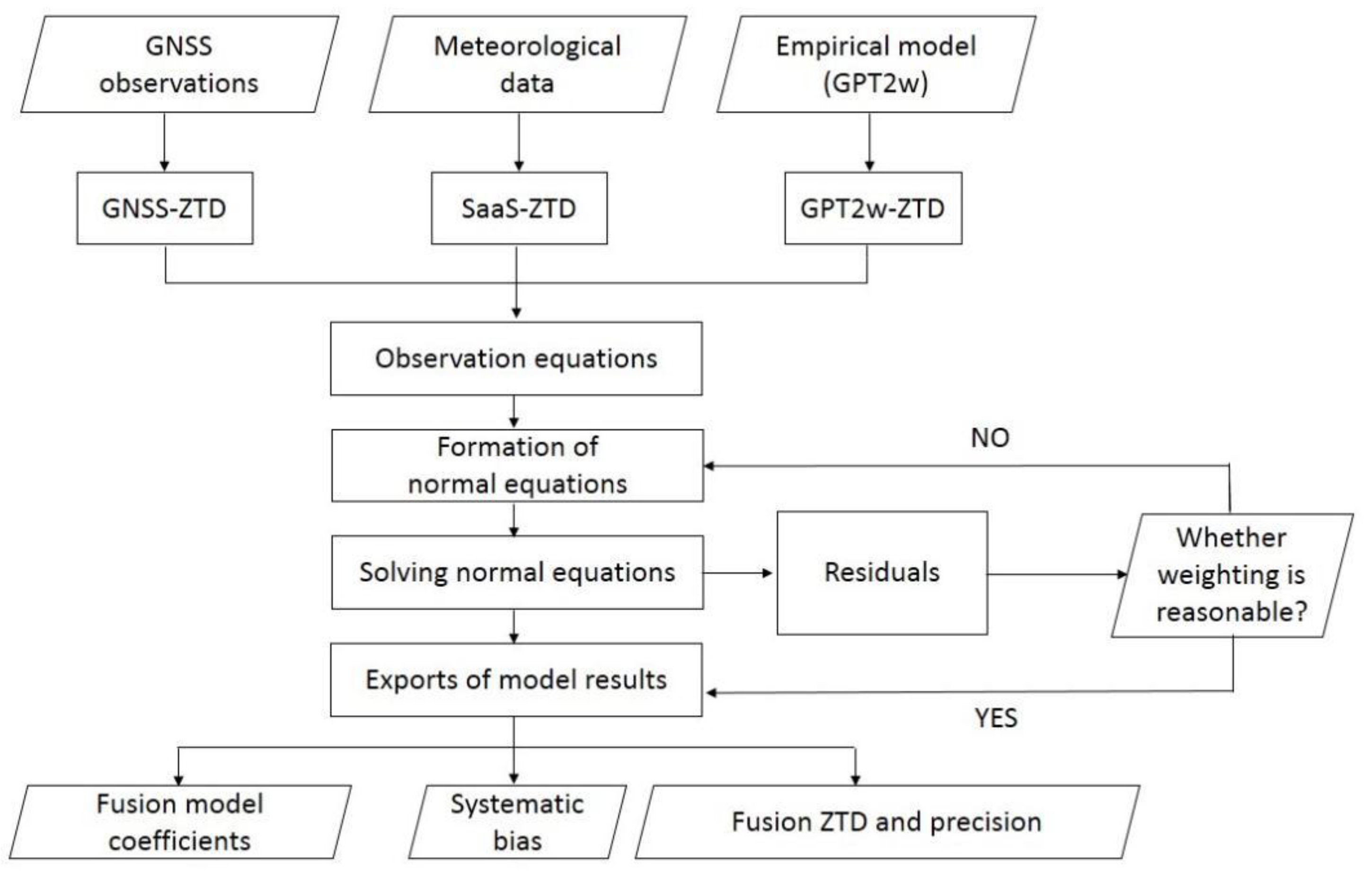
The main inputs, as well as the strategy used to accomplish the troposphere fusion modeling, are presented in the flowchart in Figure 1, in which GNSS-ZTD represents Zenith Tropospheric Delay obtained by GNSS Processing, SaaS-ZTD represents Zenith Tropospheric Delay obtained by the Saastamoinen Model, GPT2w-ZTD represents Zenith Tropospheric Delay obtained by the GPT2w Model.

2.2.2. Precise Weights Determination

The accuracy of the GNSS-based ZTD, the Saastamoinen ZTD, and the GPT2w ZTD are not consistent. During multisource data fusion, the weights of the tropospheric data from different systems need to be considered. In order to reasonably determine the weights of the types of observations, we use the following two methods:

• Helmert variance component estimation

We use this method to estimate the variance factor of various observations from a set of initial a priori variance factors, then we obtain the final weights according to this variance factor, and we conduct a final adjustment [30]. The Helmert variance component estimation formula can be written as:

$$S\hat{\theta }=W_{\theta }$$

(9)

where the specific forms of $S,\hat{\theta }$, and $W_{\theta }$, as well as the iterative calculation process, can be found in [31,32]. As the formula for the Helmert variance component estimation is very complex, matrix inversion is needed after a continuous matrix multiplication. For this reason, either of the following approximate formulas are often used in the actual calculation:

$${\hat{\sigma }}_{0_i}^2=\frac{V_i^T{P}_i{V}_i}{n_i}$$

(10)

$${\hat{\sigma }}_{0_i}^2=\frac{V_i^T{P}_i{V}_i}{n_i-tr(N^{-1}{N}_i)}$$

(11)

The iterative calculation process of the Helmert variance component estimation is as follows.

• The prior weights of the different observed values, i.e., the initial values of the weight of each type of observation (P₁, P₂, …), are assigned.
• A first adjustment is made, to obtain the values of $V_i^T{P}_i{V}_i$.
• In accordance with Equations (10) or (11) for the first-time variance component estimation, the first value of the unit weight variance ${\hat{\sigma }}_{0_i}^2$ of various observations is obtained, and then the weights are determined according to the following formula:

  $${\hat{P}}_i=\frac{c}{{\hat{\sigma }}_{0_i}^2{P}_i^{-1}}$$

  (12)

  where c is a constant. Generally, one of the ${\hat{\sigma }}_{0_i}^2$ values is selected.

The second and third steps are repeated until the unit weight variances of various observations are equal.

The three types of observations are grouped to determine the variance components in this method.

• Comprehensive weighting method

On the basis of references [19,33,34] on various troposphere models assessments, it can be concluded that the precision of the ZTD obtained from the empirical GPT2w model is the lowest (in generally ~4 cm), because the model does not consider the day cycle and the multi-peak multi-valley characteristics of the ZTD daily variation. Compared with the empirical tropospheric delay models, the precision of the Saastamoinen model is nearly the same, with normal values around 3.5 cm, however it includes information on measured meteorological parameters. The ZTD estimation of the GNSS-based model is the most accurate, with values as low as 1.5 cm, which are lower than those obtained with the other two types of troposphere models.

Considering the possibility that the Helmert variance component estimation does not take the high precision of the GNSS ZTD into account, an integrated method is proposed, which defines the initial weights according to the a priori precision. The Helmert variance component estimation is then conducted to adjust the weights with the constraint that the weight of the GNSS-derived ZTD cannot be reduced.

2.3. Data Description and Processing Strategy

Figure 2 shows on a map the locations of the continuously operating reference stations (CORS) in Hong Kong. The multisource data utilized in the troposphere fusion are listed in

Table 1. Multisource Data for the troposphere fusion model.

Data source	Period	CORS Station	Weather Station	GPT2w
				Grid Points
Hong Kong	20 July 2015~26 July 2015 1 August 2015~7 August 2015	15	14	4 (1°×1°) 21.5°~22.5° 113.5°~114.5°

.

The Hong Kong Satellite Positioning Reference Station (SatRef) CORS network consists of 15 continuously operating reference stations equipped with Leica GNSS receivers and antennas (Germany) (Figure 1). Each station (except T430) is equipped with an automatic meteorological device to record temperature, pressure and relative humidity. With these data, the hydrostatic parts of the tropospheric delay can be accurately removed. The mean horizontal distance between neighboring stations is approximately 10 km, and the ellipsoidal heights of the 15 stations are within 350 m.

Fourteen days of GNSS observation data from the CORS network were processed by the precise point positioning (PPP) module in PASSION software (China). PASSION is an after-the-fact multi-system (GPS/GLONASS/BDS/GALILEO) precise single-point positioning processing software developed by our team based in Visual Studio 2012. The international GNSS Service (IGS) RTS IGS03 orbit and clock products were used in data processing. The antenna phase center offsets and variations, phase wind-up, Earth tides, Earth rotation, ocean tides, and relativistic effects were corrected by conventional methods [35]. Differential code biases were corrected by products from the Center for Orbit Determination in Europe. The ionospheric delay was corrected to the first order by using the ionosphere-free combination of dual-frequency phase observations. The higher-order ionospheric error was neglected.

Additionally, the temperature, pressure, and relative humidity recorded by meteorological devices in 14 tracking stations were used to calculate the ZTD with the Saastamoinen model. The ZTDs in four grid points during the experimental period were provided by the GPT2w model. This paper used a total of 15 stations, of which 14 stations were recording both GPS and meteorological data. All tracking station observations had a sample rate of 30 s. The addition of the tropospheric data obtained from climatological data and the empirical model helped to improve the accuracy and reliability of the estimation. In this paper, we consider two different situations with quiet and active troposphere conditions on the day of year (DOY) 2015 201~207 and 213~219, respectively. The weather conditions on DOY 201~207 were relatively active compared with those on the preceding and following days. Several severe rainfall events occurred on these days, with the largest daily rainfall (~190 mm) of 2015 occurring on DOY 203, indicating an accumulating phase of the troposphere ZWD. However, the following days, DOY 213~219, happened to be all sunny days. For each case, we first determined the ZTD fitting coefficients, and subsequently we assessed the performance of the ZTD fusion model.

The troposphere ZTD values were chosen at an interval of 1 h between UTC 00:00 and 23:00, so that 24 samples were available for each day. As shown in Figure 2, the distribution of the CORS tracking stations is rather dense. At each sampling epoch, we used five GNSS-solved ZTD values along with the GPT2w and the Saastamoinen ZTD to determine the troposphere fitting coefficients, out of consideration of the cost of the fusion model, with the GNSS-solved ZTD from rest stations as the standard reference for evaluating the accuracies of the fusion ZTD model.

To verify the contributions of the meteorological-driven model and of the empirical model, the determination of the ZTD fitting coefficients was also conducted by using only the ZTD values obtained from 11 CORS tracking stations. This has been defined as the PPP troposphere model, the performance of which has been compared with the troposphere fusion model. In addition, the GPT2w and Saastamoinen models were used to calculate the ZTD of the CORS station. Similarly, the GNSS-derived ZTDs from CORS stations were utilized to evaluate the accuracies of the PPP troposphere model, the GPT2w model, and the Saastamoinen model along with the estimated ZTD. The optimum criterion is then defined as:

$$\begin{array}{l}bias=\frac{1}{N}{\displaystyle \sum _{i=1}^N\left(ZT{D}_i^{estimated}-ZT{D}_i^{GNSS-derived}\right)},\\ RMS=\sqrt{\frac{1}{n}{\displaystyle \sum _{i=1}^n{\left(ZT{D}_i^{estimated}-ZT{D}_i^{GNSS-derived}\right)}^2}}\end{array}$$

(13)

where $ZT{D}_i^{estimated}$ is the tropospheric delay estimated by different troposphere models, and $ZT{D}_i^{GNSS-derived}$ is the tropospheric delay obtained by GNSS processing. Two methods for determining the weights were compared by evaluating the accuracies of the fusion models with five GNSS-solved ZTD values along with the GPT2w and the Saastamoinen ZTD. In other words, we estimated the ZTD of the stations not involved in modeling with the tropospheric fitting coefficients derived from two different weights strategies, followed by an assessment of the precision of the estimated ZTD with respect to the ZTD obtained from GNSS data processing. The statistic results relative to the daily mean error are summarized in

Table 2. Comparison of fusion model accuracy with two weighting methods.

DOY	Helmert		Comprehensive
	Bias (cm)	RMS (cm)	Bias (cm)	RMS (cm)
201.00	0.00	1.33	0.04	1.28
202.00	0.35	1.84	0.22	1.73
203.00	−0.40	1.10	−0.28	1.13
204.00	−0.23	1.05	−0.06	1.05
205.00	−0.06	1.58	0.22	1.59
206.00	0.58	1.98	0.53	1.93
207.00	0.82	2.02	0.70	1.55
213.00	0.97	2.86	0.60	2.19
214.00	0.55	1.82	0.50	1.53
215.00	−0.11	1.31	0.13	1.21
216.00	−0.28	1.30	0.15	1.30
217.00	-0.62	1.97	-0.16	1.41
218.00	-0.23	1.40	-0.06	1.10
219.00	-0.12	2.71	-0.18	1.38
Mean	0.0871	1.7336	0.1679	1.4557

.

As illustrated in Table 2, the mean bias and the RMS of the comprehensive fusion model are 0.1679 cm and 1.4557 cm, respectively. The precision of this model is higher than that achieved by other methods. In contrast, the Helmert variance component estimation alone is an unreliable weighting strategy. Overall, we chose to set initial the weights according to the prior precision of the various observations. Afterwards, we determined the precise weights by the Helmert variance component estimation, keeping high values for the GNSS weights in the subsequent calculations.

3. Results and Discussion

3.1. Verification of the Systematic Bias Estimation

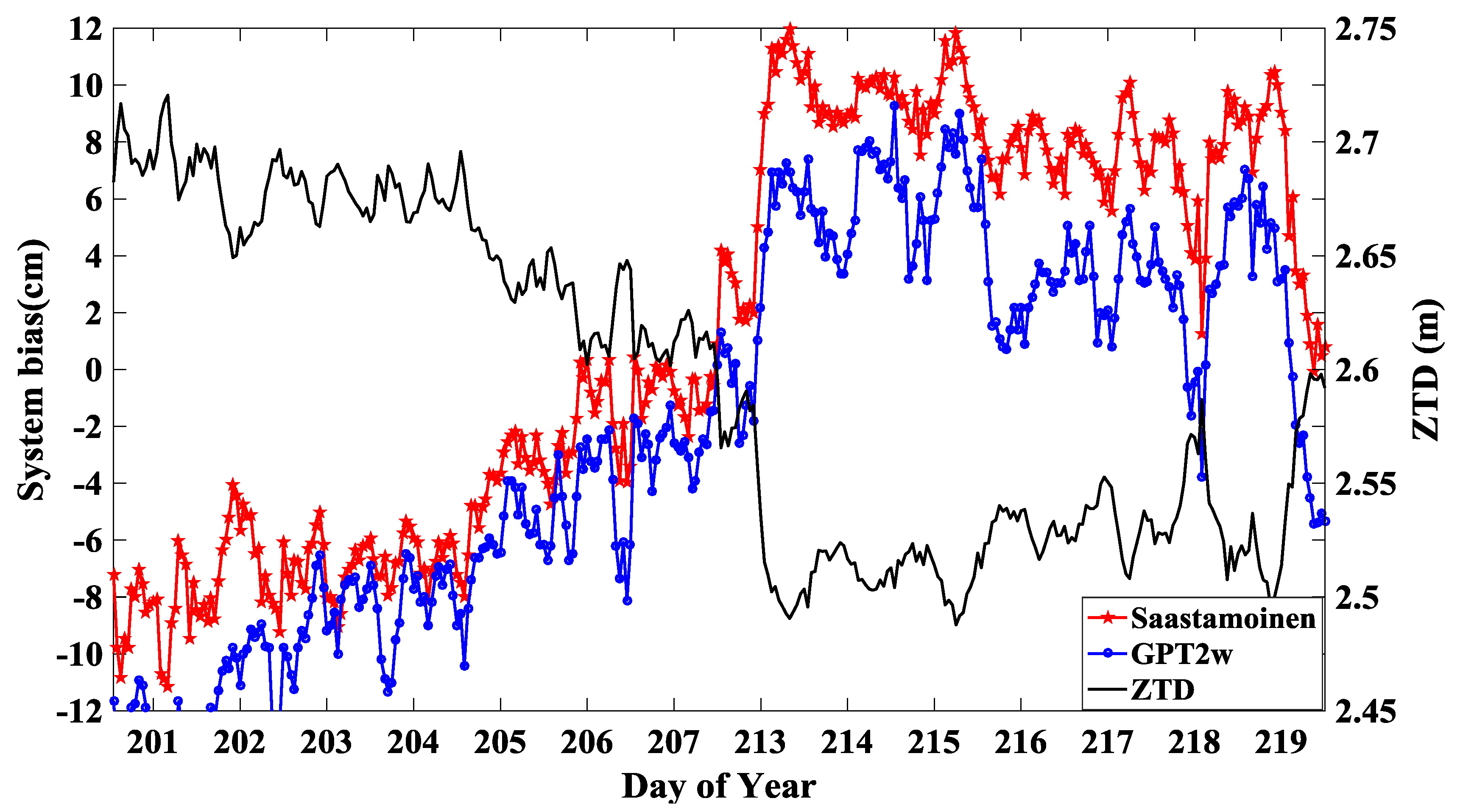
The local troposphere fusion modeling was performed hourly during the 14 days of observation in July and August. Figure 3 shows the variation of the estimated Saastamoinen and GPT2w systematic biases, and the average ZTD of the Hong Kong CORS network versus the day of the year during the July and August study periods. As seen in Figure 3, the variation of the systematic bias is related to the variation of the temporal ZTD value. During DOY 201~207, when the troposphere was experiencing continuous rainfall, an overall negative feature was identified for the systematic bias time series of the Saastamoinen and GPT2w models. This indicates that the ZTDs calculated by these models are less than the actual values in the rainy season. However, the systematic biases of the Saastamoinen and GPT2w models demonstrated a generally positive feature during DOY 213~219, indicating that the ZTD was overestimated in fair weather. In addition, the correlation coefficient between the systematic bias of the GPT2w model and the ZTD value is –0.9781 cm, while it reaches -0.9974 cm for the Saastamoinen model, showing that systematic biases are significantly affected by tropospheric conditions. In general, the systematic bias is larger when the troposphere delays are extremely large in rainfall events, or relatively smaller in the sunny days August. Furthermore, the systematic bias of the GPT2w model is larger than that in the Saastamoinen model in the active troposphere period, but smaller than that in the Saastamoinen model in quiet tropospheric conditions. However, there also exist some sudden changes, the cause of which deserves further research. So far, this paper has only concerned the systematic bias variation within a short period. However, the systematic deviation trend of each model requires long-term historical data, to be verified in future studies.

3.2. Verification of the Zenith Tropospheric Delay

3.2.1. Active Troposphere Condition

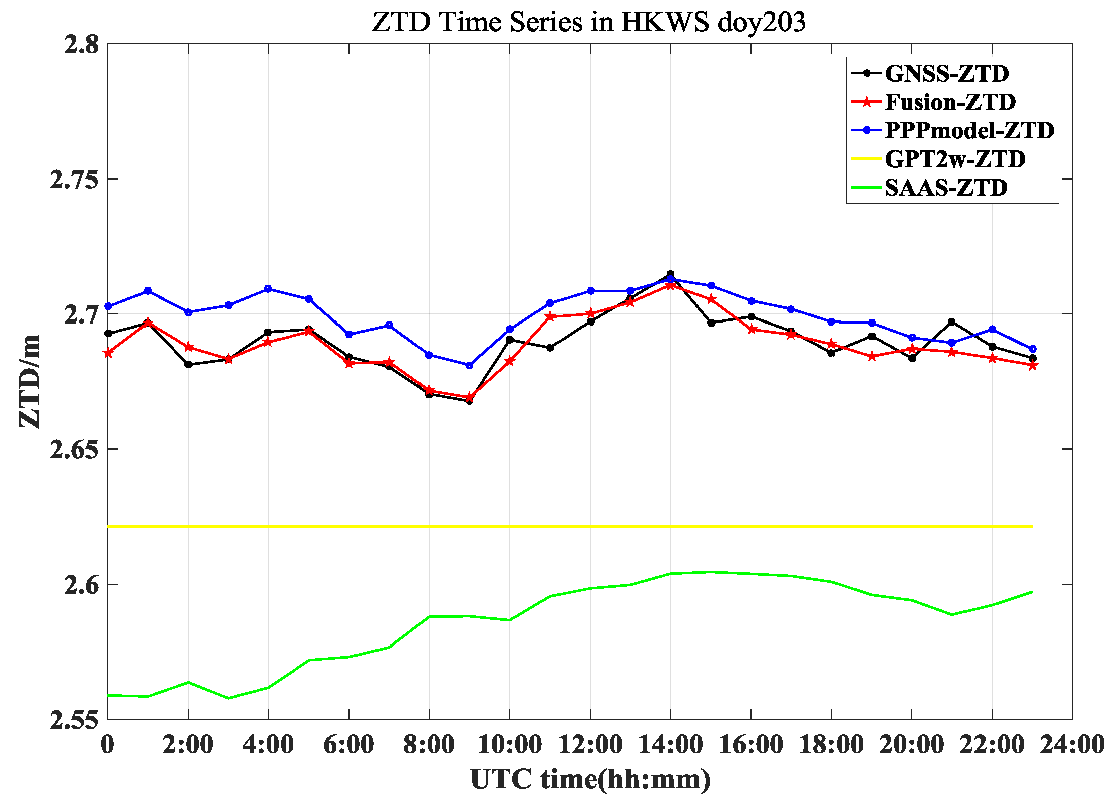
The local troposphere fusion modeling was performed every hour during the 7-day period in July. As an independent reference, the ZTD values derived from GNSS data processing of CORS stations that were not involved in modeling were used to assess the tropospheric fusion model. The GNSS-solved ZTD series at station HKWS are shown as an example in Figure 4. For the purpose of comparison, the ZTD values estimated by the fusion model, by the PPP model, and by other models at HKWS station on DOY 203 are also illustrated. As shown in Figure 4, the GNSS-based ZTD values match the fusion estimated ZTD values quite well, with a maximum discrepancy of approximately 1 cm.

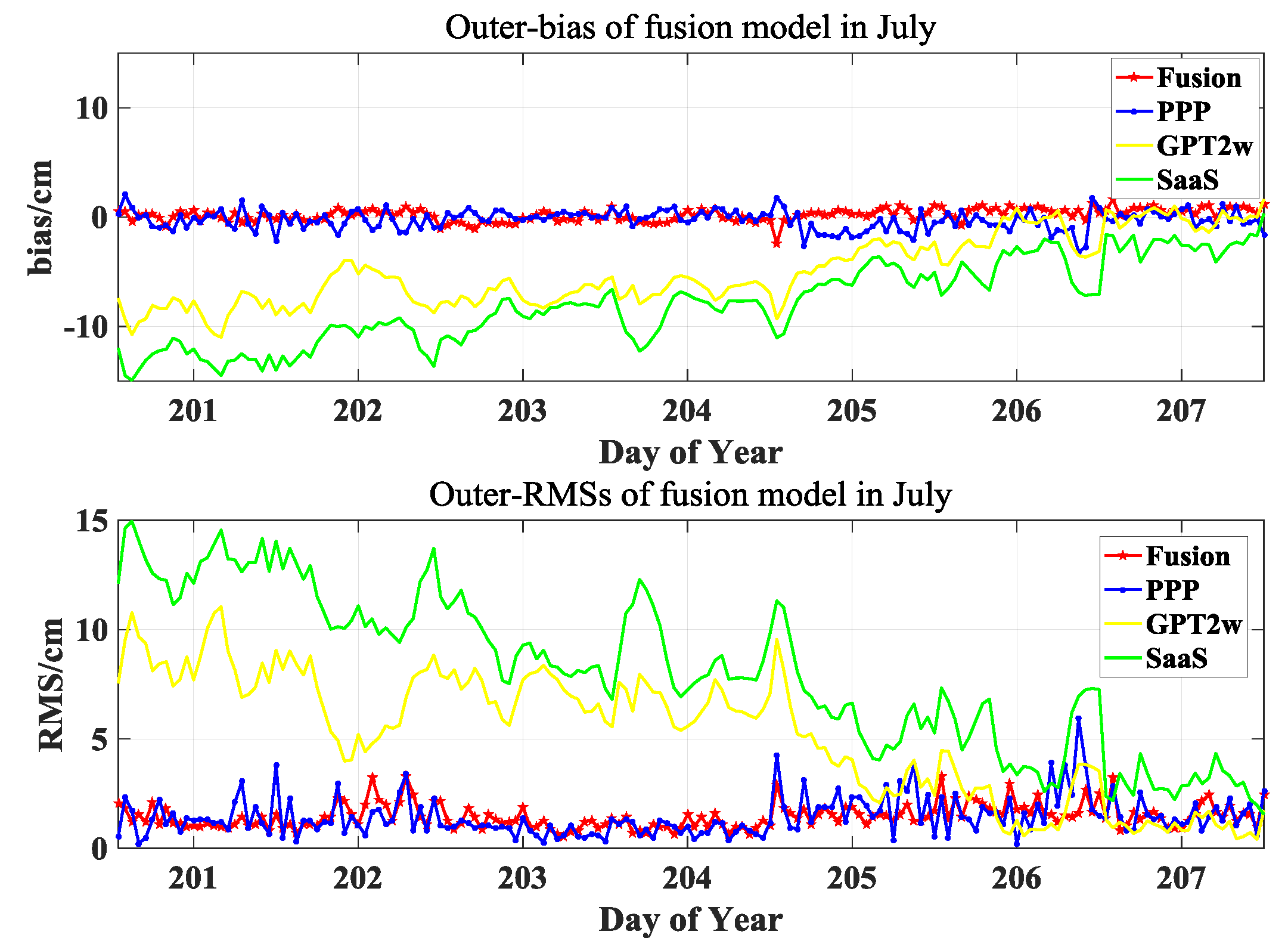
For the active troposphere period assessed, time series of the mean differences and of the corresponding standard deviations over the network are presented in Figure 5 for different troposphere models.

During DOY 201~207, the bias of SAAS-ZTD fluctuated from -14.92 cm to 0.31 cm, while the RMS ranged from 1.56 cm to 14.96 cm, pointing out that the ZTD values are particularly unreliable during heavy rainfall. The reason for the poor accuracy is related to the imprecise Saastamoinen ZTD calculation formula itself. Moreover, the weather parameters in the Saastamoinen formula are not instantly updated, making the meteorological model relatively inaccurate, especially in active troposphere conditions.

The bias of the GPT2w-ZTD estimation is −10.99~1.63 cm, while the RMS is 0.41~11.05 cm. As in the Saastamoinen model, the error is much larger during major rainfalls. Since the GPT2w model is an empirical model and does not take the ZTD daily variation into consideration, the provided ZTD value remains unchanged within one day. Therefore, the GPT2w model accuracy is especially poor in the active tropospheric condition.

Unlike empirical and meteorological models, the precision of the PPP model is considerably reliable. The bias value is –3.22~1.60 cm while the RMS is within 0.18~3.32 cm. These values are comparable with those of the deviation of the fusion model, which exhibit the highest precision. The bias of the ZTD derived from the fusion model fluctuates between –2.41 cm and 1.60 cm, and the minimum RMS is 0.52 cm, while the maximum RMS is 3.32 cm. As shown in Figure 5, the fusion model maintains high precision and stability in active tropospheric conditions.

According to the optimum criterion (13), the ZTD precision for each day has been determined and is listed in

Table 3. Daily mean precision (cm) of troposphere models in July.

DOY	Fusion-Model		PPP-Model		GPT2w		SAAS
	bias	RMS	bias	RMS	bias	RMS	bias	RMS
201	0.04	1.28	−0.19	1.43	−8.59	8.66	−13.02	13.10
202	0.27	1.82	−0.44	1.43	−6.55	6.59	−11.08	11.22
203	−0.29	1.15	0.14	0.81	−7.12	7.17	−8.90	9.04
204	−0.06	1.04	0.20	0.89	−6.52	6.57	−8.67	8.78
205	0.22	1.60	−0.93	2.03	−3.99	4.11	−6.10	6.41
206	0.52	1.91	−0.55	2.01	−1.83	2.27	−4.75	5.11
207	0.70	1.56	−0.05	1.51	−0.01	1.03	−2.37	2.90
mean	0.20	1.48	−0.26	1.44	−4.94	5.20	−7.84	8.08

. The deviations between the estimated ZTD from different models and the GNSS-derived ZTD are calculated as well.

In general, the accuracy of the ZTD model that combines three data sources is significantly better than that of the GPT2w model and the SAAS model. Compared to the PPP model, the fusion model reaches an equivalent accuracy and requires less CORS stations. Clearly, the troposphere fusion model reduces the modeling cost significantly and improves the spatial resolution of the PPP-ZTD.

3.2.2. Quiet Troposphere Condition

The second case study describes a stable troposphere period during a seven-day period in August, when the daily sunshine time reached 5.7~11.4 h.

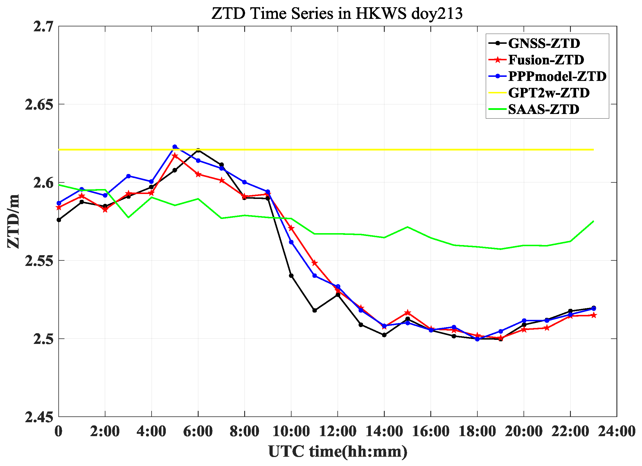
As in the processing and strategies used in the first case study, the series derived from GNSS processing and the ZTD values estimated by various models at station HKWS on DOY 213 are again taken as an example in Figure 6. The figure demonstrates a descending pattern for the tropospheric delay in sunny days. The ZTD oscillates around a constant value during sunny days, whereas it remains at a high value during rainfalls. Compared with GNSS-solved ZTD values, the values estimated from the fusion model show a maximum discrepancy of approximately 3 cm, and an average discrepancy of 0.29 cm.

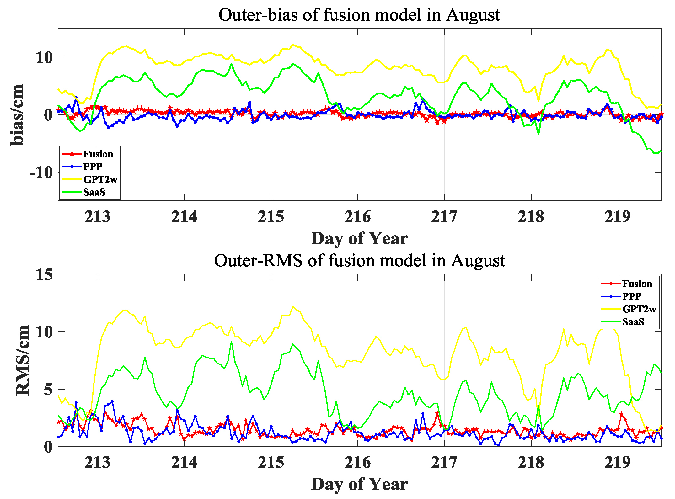
In Figure 7, the time series of the mean difference are shown, as well as the corresponding standard deviations over the network for the fusion model, the PPP model, and other models for the quiet troposphere period.

Unlike the relatively negative pattern seen in the bias time series on DOY 201~207, an overall positive trend has been identified for the bias time series of the GPT2w and Saastamoinen models during DOY 213~219, which indicates that the empirical and meteorological troposphere delay are overestimated in fair weather. The biases of the SAAS-ZTD values are between -6.76 cm and 8.83 cm, the minimum RMS is 1.41 cm, and the maximum is 9.16 cm. The accuracy of the Saastamoinen tropospheric delay model during the steady troposphere condition is higher than that during the active period.

As for the ZTD obtained from the GPT2w model, the bias fluctuates in the range 1.14~12.17 cm, and the RMS values vary from 1.29 cm to 12.19 cm. Among the various models, these values indicate that the GPT2w model has the worst accuracy during the steady period.

The accuracy of the PPP model, in which modeling is carried out with GNSS-derived ZTD values alone, is much better than that of the GPT2w model. The bias fluctuated from -2.18 to 2.97 cm, and the RMS values varied from 0.14 to 3.92 cm. Introducing empirical and meteorological tropospheric data into GNSS data has a stabilizing effect on the deviation of the fusion model, with the bias of the estimated ZTD varying from -1.35 cm to 1.41 cm. In addition, the RMS values remained between 0.54 cm and 3.16 cm. As a result, the accuracy of the fusion model is comparable to the accurate PPP model during the calm troposphere condition.

In

Table 4. Daily mean precision (cm) of troposphere models in August.

DOY	Fusion-Model		PPP-Model		GPT2w		SAAS
	bias	RMS	bias	RMS	bias	RMS	bias	RMS
213	0.61	2.20	−0.26	2.01	7.37	7.47	2.79	4.44
214	0.49	1.49	−0.56	1.49	9.72	9.75	5.68	5.88
215	0.14	1.20	−0.15	1.03	10.15	10.18	6.34	6.57
216	0.16	1.32	0.15	1.15	8.07	8.11	2.64	3.27
217	−0.16	1.41	0.24	1.12	7.75	7.87	2.98	3.87
218	−0.04	1.08	−0.09	0.90	7.09	7.16	2.04	3.49
219	−0.24	1.42	−0.16	0.86	6.34	6.40	0.08	4.87
mean	0.14	1.45	−0.12	1.22	8.07	8.13	3.22	4.63

, the mean precision values over the monitoring station network for each day are listed. The deviations between various troposphere models and the ZTD calculated by GNSS processing are reported as well.

Similar to the first case study, the best performance is provided by the fusion model. The mean RMS of the fusion model is 1.45 cm, which is significantly lower than that of the GPT2w model (8.13 cm) and the SAAS model (4.63 cm). The accuracy of the ZTD model using multisource data substantially exceeds that of the GPT2w model and the SAAS model. In addition, the accuracy of the model is comparable to that of the PPP model, which uses data from 11 CORS stations. Fortunately, the construction costs and the usage of related human and material resources are reduced by introducing experiential and meteorological data into the model.

3.3. Impact of the dDstribution of Modeling Station Elevations on Model Precision

To analyze the spatial distribution characteristic of the fusion model precision, the daily mean and standard deviation differences are calculated for each station, with the elevation of five modeling sites and the precision at certain high stations given in

Table 5. Precision of the local troposphere fusion model for each station.

DOY	Site Involved in Modeling					HKNP		HKST
						bias	RMS	bias	RMS
201	HKKS(44.69 m)	HKKT(34.54 m)	HKLM(8.53 m)	HKLT(125.90 m)	HKMW(194.94 m)	2.10	2.75	1.29	1.64
202	HKKS(44.69 m)	HKKT(34.54 m)	HKLM(8.53 m)	HKLT(125.89 m)	HKMW(194.94 m)	3.91	4.68	2.34	2.75
203	HKKS(44.69 m)	HKKT(34.54 m)	HKLT(125.89 m)	HKMW(194.94 m)	HKNP(350.67 m)	0.27	0.37	0.85	1.43
204	HKKS(44.69 m)	HKKT(34.54 m)	HKLM(8.53 m)	HKLT(125.89 m)	HKNP(350.67 m)	0.41	0.44	1.44	2.11
205	HKKS(44.69 m)	HKKT(34.54 m)	HKLM(8.53 m)	HKLT(125.89 m)	HKMW(194.94 m)	2.83	3.04	2.17	2.40
206	HKKS(44.69 m)	HKKT(34.54 m)	HKLM(8.53 m)	HKLT(125.89 m)	HKMW(194.94 m)	3.91	4.71	2.60	2.90
207	HKKS(44.69 m)	HKKT(34.54 m)	HKLM(8.53 m)	HKLT(125.89 m)	HKMW(194.94 m)	1.89	3.44	2.60	2.82
213	HKKS(44.69 m)	HKKT(34.54 m)	HKLM(8.53 m)	HKLT(125.89 m)	HKMW(194.94 m)	3.74	5.61	3.26	3.49
214	HKKS(44.69 m)	HKKT(34.54 m)	HKLM(8.53 m)	HKLT(125.89 m)	HKMW(194.94 m)	3.36	3.94	2.44	2.73
215	HKKS(44.69 m)	HKKT(34.54 m)	HKLM(8.53 m)	HKLT(125.89 m)	HKNP(350.67 m)	0.03	0.04	2.20	2.73
216	HKKS(44.69 m)	HKKT(34.54 m)	HKLM(8.53 m)	HKLT(125.89 m)	HKNP(350.67 m)	0.04	0.06	2.09	2.69
217	HKKS(44.69 m)	HKKT(34.54 m)	HKLM(8.53 m)	HKLT(125.89 m)	HKNP(350.67 m)	0.01	0.04	1.23	2.47
218	HKKS(44.69 m)	HKKT(34.54 m)	HKLM(8.53 m)	HKLT(125.89 m)	HKNP(350.67 m)	0.00	0.03	1.21	1.96
219	HKKS(44.69 m)	HKKT(34.54 m)	HKLM(8.53 m)	HKLT(125.89 m)	HKNP(350.67 m)	0.01	0.02	-1.43	2.95

. According to the statistical results, the troposphere ZTD fitting precisions are optimal on DOY 203 because of the uniformly distributed network configurations. The bias and the RMS are less than 1 mm in most stations, as shown in

Table 6. Precision of the local troposphere fusion model for each station on DOY203.

Station	Height (m)	DOY203
		bias	RMS
HKKS	44.692	0.13	0.40
HKKT	34.538	−0.59	0.73
HKLT	125.89	0.02	0.42
HKMW	194.936	0.17	0.29
HKNP	350.666	0.27	0.37
HKOH	166.375	0.69	1.48
HKPC	18.083	−1.03	1.50
HKSC	20.204	−0.56	1.17
HKSL	95.266	0.42	0.56
HKSS	38.684	−0.66	0.89
HKST	258.687	0.85	1.43
HKTK	22.497	−1.09	1.35
HKWS	63.762	−0.08	0.52
T430	41.29	-1.10	1.20

. On the other hand, the estimated ZTDs at stations at high elevation such as HKNP and HKST are less accurate when the elevations of the modeling stations are uneven. The largest RMS reaches 5.61 cm, while it is 3.49 cm on DOY 213, when all observation stations were below 200 m.

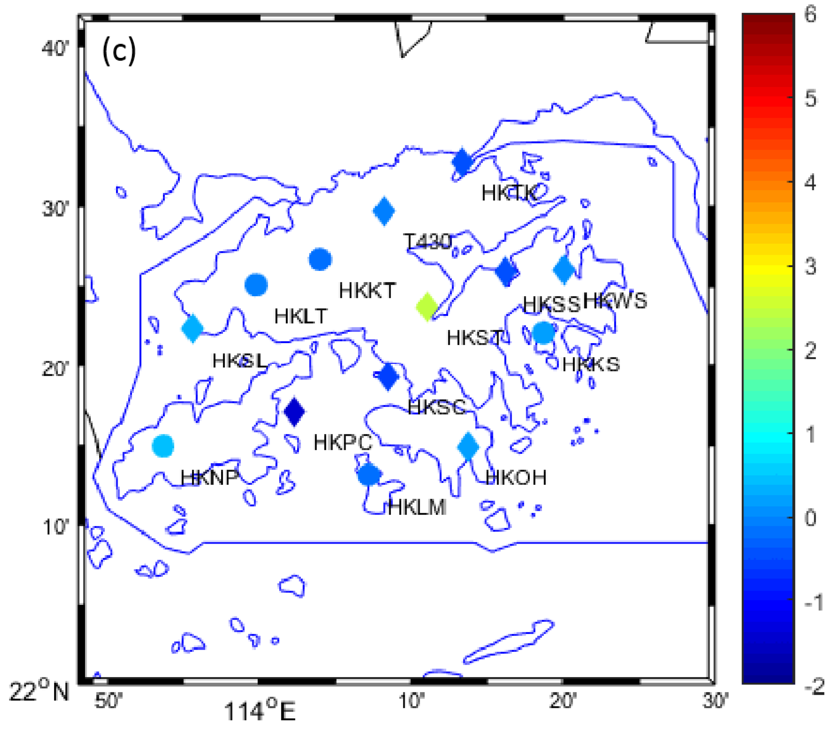
Typical ZTD differences between the fusion model and the GNSS-derived ZTD at CORS station locations on UTC 12:00 from DOY 202 to 204 are presented in Figure 8. This example shows that the ZTDs derived from the fusion model are consistent with those obtained by GNSS. However, the spatial distribution of the fusion model accuracy is different due to the specific CORS station configurations involved in modeling at different time periods. The results on DOY 202 present a maximum difference of 5.14 cm, versus 1.65 cm on DOY 203, and 2.50 cm on DOY 204. In this example, the bias values at HKNP and HKST stations on DOY 202 are obviously larger than those at other stations. It can be noticed that the elevations of HKNP and HKST stations are significantly higher than those of the other stations, while the elevation of the five stations involved in modeling is generally below 200 m. This relatively low-elevation network configuration accounts for the inaccurate reduction in elevation of the fusion models at high-elevation sites. In contrast, the stations participating in modeling on DOY 203, having uniformly-distributed elevations, make the fusion model have high accuracy across the whole Hong Kong CORS network, in which the minimum daily average RMS reached 0.52 cm at HKWS station. Although the elevation of the modeling stations on DOY 204 varied from 8.53 m to 350.66 m, the uneven elevation intervals led to a relatively large deviation at HKST station. Therefore, the elevation distribution should be taken into consideration for establishing the most accurate fusion model.

4. Conclusions

The GNSS data processing can provide values of zenith troposphere delay with high accuracy on a global scale. However, the development of models of the troposphere is still limited by the uneven distribution and high cost of CORS stations. In order to reduce the modeling expense but at the same time guarantee the accuracy of tropospheric delay estimations, this paper proposes a local troposphere fusion method to improve the accuracy and reliability of the regional tropospheric delay model in GNSS tracking station missing areas. A real-time local troposphere fitting model is proposed in this paper. By adding ZTD data obtained from the meteorological Saastamoinen model and the empirical GPT2w model, a troposphere fusion model with high spatial-temporal resolution and low cost is established. Taking into account the different accuracy of various tropospheric data, the Helmert variance component estimation method and prior precision knowledge are used to determine the precise weight for all types of observational data. Furthermore, the systematic biases of the Saastamoinen and GPT2w models with respect to GNSS observations are taken into consideration, and are estimated together with the tropospheric delay model fitting parameters by least squares.

The proposed method has been evaluated using a Hong Kong SatRef CORS network under active and quiet troposphere conditions on DOY 2015 201~207 and 213~219, respectively. As an external reference and partial data source for modeling, 14 days of GNSS observation data from the SatRef Network are processed by the precise point positioning (PPP) module in PASSION software to assess the performance of the tropospheric fusion model. In addition, the comparison of the accuracies is also conducted with respect to the PPP model relying only on GNSS observations. The fusion-modeled ZTDs present an accuracy of approximately 1.48 cm in the active troposphere condition, and 1.45 cm in the stable troposphere condition when compared to the GNSS-derived ZTDs. This performance is significantly better than that of the conventional tropospheric GPT2w and Saastamoinen models (i.e., 5.20 cm and 8.08 cm in July, respectively, and 8.13 cm and 4.63 cm in August, respectively). Similar performances to that of the fusion model are achieved by the PPP model (i.e., 1.44 cm and 1.22 cm in July and August, respectively). However, compared with the PPP model which includes data from 11 CORS stations, the fusion model only relies on GNSS stations yet it remains stable and reliable also during the active tropospheric condition.

The accuracy and spatial resolution of the troposphere model in a sparse CORS network has improved to some extent after introducing meteorological and empirical data, particularly in remote areas. If the elevations of the stations are evenly distributed, the quality of the tropospheric fusion model will be improved further.

This paper only concerned the scale of the urban CORS network with a small coverage. More efforts will be made in order to produce a ZTD fitting model the determination of provincial or national level CORS networks, i.e., with larger coverage, in the future.

References

- Yao, Y.; Xu, X.; Xu, C.; Peng, W.; Wan, Y. GGOS tropospheric delay forecast product performance evaluation and its application in real-time PPP. J. Atmos. Sol.-Terr. Phys. 2018, 175, 1–17. [Google Scholar] [CrossRef]
- Kim, J.; Song, J.; No, H.; Han, D.; Kim, D.; Park, B.; Kee, C. Accuracy Improvement of DGPS for Low-Cost Single-Frequency Receiver Using Modified Flächen Korrektur Parameter Correction. ISPRS Int. J. Geo-Inf. 2017, 6, 222. [Google Scholar] [CrossRef]
- Ahn, Y.W.; Kim, D.; Dare, P. Local tropospheric anomaly effects on GPS RTK performance. Proc. ION GNSS 2006, 2006, 1925–1935. [Google Scholar]
- Song, J.; Park, B.; Kee, C. Comparative Analysis of Height-Related Multiple Correction Interpolation Methods with Constraints for Network RTK in Mountainous Areas. J. Navig. 2016, 69, 991–1010. [Google Scholar] [CrossRef] [Green Version]
- Collins, J.P.; Langley, R. The residual tropospheric propagation delay: How bad can it get? In Proceedings of Ion gps. Inst. Navig. 1998, 11, 729–738. [Google Scholar]
- Collins, J.P.; Langley, R.B. A Tropospheric Delay Model for the User of the Wide Area Augmentation System; Department of Geodesy and Geomatics Engineering, University of New Brunswick: Fredericton, NB, USA, 1997. [Google Scholar]
- MOPS, W. Minimum Operational Performance Standards for Global Positioning System/Wide Area Augmentation System Airborne Equipment; RTCA Inc.: Washington, DC, USA, 1999; Documentation No. RTCA/DO-229B, 6. [Google Scholar]
- Penna, N.; Dodson, A.; Chen, W. Assessment of EGNOS Tropospheric Correction Model. J. Navig. 2001, 54, 37–55. [Google Scholar] [CrossRef] [Green Version]
- Ueno, M.; Hoshinoo, K.; Matsunaga, K.; Kawai, M.; Nakao, H.; Langley, R.B.; Bisnath, S.B. Assessment of atmospheric delay correction models for the Japanese MSAS. In Proceedings of the 14th International Technical Meeting of the Satellite Division of The Institute of Navigation (ION GPS 2001), Salt Lake City, UT, USA, 11–14 September 2001; pp. 2341–2350. [Google Scholar]
- Boehm, J.; Heinkelmann, R.; Schuh, H.; Böhm, J. Short Note: A global model of pressure and temperature for geodetic applications. J. Geod. 2007, 81, 679–683. [Google Scholar] [CrossRef]
- Kouba, J. Testing of global pressure/temperature (GPT) model and global mapping function (GMF) in GPS analyses. J. Geod. 2009, 83, 199–208. [Google Scholar] [CrossRef]
- Petit, G.; Luzum, B. IERS conventions 2010, IERS Technical Note; IERS Conventions Centre: Paris, France, 2010. [Google Scholar]
- Lu, C.; Zus, F.; Ge, M.; Heinkelmann, R.; Dick, G.; Wickert, J.; Schuh, H. Tropospheric delay parameters from numerical weather models for multi-GNSS precise positioning. Atmos. Meas. Techn. 2016, 9, 5965–5973. [Google Scholar] [CrossRef] [Green Version]
- Lagler, K.; Schindelegger, M.; Böhm, J.; Krásná, H.; Nilsson, T. GPT2: Empirical slant delay model for radio space geodetic techniques. Geophys. Lett. 2013, 40, 1069–1073. [Google Scholar] [CrossRef] [Green Version]
- Böhm, J.; Möller, G.; Schindelegger, M.; Pain, G.; Weber, R. Development of an improved empirical model for slant delays in the troposphere (GPT2w). GPS Solut. 2014, 19, 433–441. [Google Scholar] [CrossRef] [Green Version]
- Hopfield, H.S. Two-quartic Tropospheric Refractivity Profile for Correcting Satellite Data. J. Geophys. Res. 1969, 74, 4487–4499. [Google Scholar] [CrossRef]
- Saastamoinen, J. Atmospheric Correction for Troposphere and Stratosphere in Radio Ranging of Satellites. Use Artif. Satell. Geod. 1972, 15, 247–251. [Google Scholar]
- Black, H.D. An easily implemented algorithm for the tropospheric range correction. J. Geophy. Res. Solid Earth 1978, 83, 1825–1828. [Google Scholar] [CrossRef]
- Qu, W.; Zhu, W.; Song, S.; Ping, J. Three kinds of tropospheric delay correction model accuracy evaluation. J. Astron. 2008, 49, 113–122. [Google Scholar]
- Tao, W. Near real-time GPS PPP-inferred water vapor system development and evaluation. Master’s Thesis, Department of Geomatics Engineering, University of Calgary, Calgary, AB, Canada, 2008. [Google Scholar]
- Ye, S.; Zhang, S.; Liu, J. Precision single point positioning method is used to estimate the accuracy of tropospheric delay. J. Wuhan Univ. (Inf. Sci. Ed.) 2008, 33, 788–791. [Google Scholar]
- Wang, M.; Chai, H.; Xie, K.; Chen, Y. PWV inversion based on CNES realtime orbits and clocks. J. Geod. Geodyn. 2013, 33, 137–140. [Google Scholar]
- Shi, J.; Xu, C.; Guo, J.; Gao, Y. Local troposphere augmentation for real-time precise point positioning. Earth Planets Space 2014, 66, 1–13. [Google Scholar] [CrossRef]
- Douša, J.; Václavovic, P.; Zhao, L.; Kačmařík, M. New adaptable all-in-one strategy for estimating advanced tropospheric parameters and using real-time orbits and clocks. Remote Sens. 2018, 10, 232. [Google Scholar] [CrossRef]
- Douša, J.; Eliaš, M.; Václavovic, P.; Eben, K.; Krč, P. A two-stage tropospheric correction model combining data from GNSS and numerical weather model. GPS Solut. 2018, 22, 77. [Google Scholar] [CrossRef]
- Rocken, C.; Ware, R.; Hove, T.V.; Solheim, F.; Alber, C.; Johnson, J.; Bevis, M.; Businger, S. Sensing atmospheric water vapor with the global positioning system. Geophys. Res. Lett. 2013, 20, 2631–2634. [Google Scholar] [CrossRef]
- Ifadis, I.I. The Atmospheric Delay of Radio Waves: Modeling the Elevation Dependence on a Global Scale; Technical Report No. 38L; Chalmers, U. of Technology: Goteburg, Sweden, 1986. [Google Scholar]
- Askne, J.; Nordius, H. Estimation of Tropospheric Delay for Mircowaves from Surface Weather Data. Radio Sci. 1987, 22, 379–386. [Google Scholar] [CrossRef]
- Thayer, G.D. An improved equation for the radio refractive index of air. Radio Sci. 1974, 9, 803–807. [Google Scholar] [CrossRef]
- Teunissen, P.J.G.; Amiri-Simkooei, A.R. Least-squares variance component estimation. J. Geod. 2008, 82, 65–82. [Google Scholar] [CrossRef]
- Grafarend, E.; Kleusberg, A.; Schaffrin, B. An introduction to the variance-covariance component estimation of Helmert type. Zeitschrift für Vermessungswesen 1980, 105, 161–180. [Google Scholar]
- Cui, X.Z.; Yu, Z.C.; Tao, B.Z.; Liu, D.J. Generalized Surveying Adjustment (New Edition); Wuhan University Press: Wuhan, China, 2005. [Google Scholar]
- Chen, Q.; Song, S.; Heise, S.; Liou, Y.; Zhu, W.; Zhao, J. Assessment of ZTD derived from ECMWF/NCEP data with GPS ZTD over China. GPS Solut. 2011, 15, 415–425. [Google Scholar] [CrossRef]
- Hua, Z.; Liu, L.; Liang, X. An Assessment of GPT2w Model and Fusion of a Troposphere Model with in Situ Data; Geomatics & Information Science of Wuhan University: Wuhan, China, 2017. [Google Scholar]
- Kouba, J.; Héroux, P. Precise Point Positioning Using IGS Orbit and Clock Products. GPS Solut. 2001, 5, 12–28. [Google Scholar] [CrossRef]
Figure 1.
Flowchart of troposphere fusion modeling.
Figure 2.
The Continuously Operating Reference Stations in Hong Kong.
Figure 3.
Time series of daily average ZTD in Hong Kong and Systematic bias of Saastamoinen and GPT2w model in two cases.
Figure 4.
GNSS-derived and estimated ZTD by kinds of models at station HKWS on DOY203.
Figure 5.
Bias and RMS of each troposphere model in July.
Figure 6.
GNSS-derived and estimated ZTD by the kinds of models at station HKWS on DOY213.
Figure 7.
Bias and RMS of each troposphere model in August.
Figure 8.
(a–c) Differences (cm) between ZTDs provided by the fusion model and GNSS processing on the day 202/203/204 UTC 12:00.