Global Mean Sea Surface Height Estimated from Spaceborne Cyclone-GNSS Reflectometry

Abstract

Mean sea surface height (MSSH) is an important parameter, which plays an important role in the analysis of the geoid gap and the prediction of ocean dynamics. Traditional measurement methods, such as the buoy and ship survey, have a small cover area, sparse data, and high cost. Recently, the Global Navigation Satellite System-Reflectometry (GNSS-R) and the spaceborne Cyclone Global Navigation Satellite System (CYGNSS) mission, which were launched on 15 December 2016, have provided a new opportunity to estimate MSSH with all-weather, global coverage, high spatial-temporal resolution, rich signal sources, and strong concealability. In this paper, the global MSSH was estimated by using the relationship between the waveform characteristics of the delay waveform (DM) obtained by the delay Doppler map (DDM) of CYGNSS data, which was validated by satellite altimetry. Compared with the altimetry CNES_CLS2015 product provided by AVISO, the mean absolute error was 1.33 m, the root mean square error was 2.26 m, and the correlation coefficient was 0.97. Compared with the sea surface height model DTU10, the mean absolute error was 1.20 m, the root mean square error was 2.15 m, and the correlation coefficient was 0.97. Furthermore, the sea surface height obtained from CYGNSS was consistent with Jason-2′s results by the average absolute error of 2.63 m, a root mean square error ($\mathrm{RMSE}$) of 3.56 m and, a correlation coefficient ($R$) of 0.95.

1. Introduction

About three-quarters of the Earth’s surface is covered by the sea, and the rise of sea level affects the survival of the land and tropical coastal areas. These changes will bring huge economic losses and human casualties [1]. Meanwhile, the mean sea surface height (MSSH) is one of the concerns of marine science and environmental science, which is widely used by geodesists and geophysicists to analyze the geoid gap, Earth’s internal dynamic mechanism, and the prediction of ocean dynamics. Oceanographers use the mean sea surface as a reference to study sea surface height, ocean circulation and other issues [2,3]. Traditional ocean observation methods, such as ship survey, buoy and coastal monitoring station, have high cost, sparse data and poor repeatability, while altimetry satellites only measure subsatellite points with low spatial and temporal resolution, and cannot obtain ocean information with large spatial scale in a short time range [4]. As early as 1968, Barrick et al. (1968) studied and obtained the scattering characteristics of rough surfaces [5].

In 1988, Hall and Cordey proposed the use of Global Positioning System (GPS) reflected signals to detect the state of the sea. Subsequently, Martin-Neira first proposed the use of GPS reflected signal for marine altimetry, which was also the first application of Global Navigation Satellite System-Reflectometry (GNSS-R) [4]. Furthermore, more and more researches have advanced the analysis of reflections of a physical mechanism, observation instruments, the physical geometric parameter inversion method, and their performances, which has explored the advantages of passive multi-base static GNSS-R over active single-base static spatial altimetry [6,7,8]. Pia Addabbo et al. [9] designed a flexible and extensible simulator, which is useful for understanding the results of real delay Doppler maps (DDMs). Specifically, they identified reductions in airborne energy requirements, system complexity, and cost of passive GNSS reflectance measurement receivers and increased coverage by simultaneously tracking reflected signals from multiple GNSS satellites [10]. Meanwhile, the past GNSS-R experiments mainly focused on receiver experiments on land and coast, which demonstrated new applications of GNSS reflection measurement, such as altimetry, tide monitoring, soil moisture, sea surface roughness [11], and wind speed measurement [12]. Space-based experiments have been carried out with some demonstrations, e.g., TechDemoSat-1 (TDS-1) missions [13,14].

The spaceborne Cyclone Global Navigation Satellite System (CYGNSS) mission was launched on 15 December 2016. The CYGNSS mission with eight satellites is increasingly interesting, measuring ocean height from space using reflected GNSS signals, which provide a new opportunity to estimate MSSH in all weathers, with global fast coverage, high spatial–temporal resolution, rich signal sources, and strong concealability. The CYGNSS has higher antenna gain (14.5 dB) and more channels. Li et al. [15] used the data of CYGNSS to assesses the ocean altimetry performance and showed the precision of SSH up to 2.5 m. In this paper, the global mean sea surface height is the first time estimated from space-borne CYGNSS DDM data. The accuracy and reliability of MSSH estimation are analyzed and validated. In Section 2, CYGNSS observations and data processing are presented. Section 3 presents the results and analysis. Finally, conclusions are given in Section 4.

2. Observations and Data Processing

2.1. CYGNSS

The CYGNSS was jointly developed by National Aeronautics and Space Administration (NASA), the University of Michigan, and the Southwest Research Institute of the United States. The CYGNSS consists of eight identical tiny satellites, which were launched into orbit on 15 December 2016 by Alliant Techsystems Ins (ATK), an l-1011 aircraft, using an air-launched Pegasus rocket XL. Compared with the previous TDS-1 satellite, the CYGNSS is specially used for GNSS reflection measurement. It is only equipped with a Space GPS Receiver Remote Sensing Instrument (SGR-ReSI) and has no other redundant payloads. The CYGNSS with eight small satellites improves the observation data of space and time resolution, with each satellite weighing at 24 kg, an orbital inclination of 35°, and altitude of 510 km, and 37-watt power for each satellite, and every tiny satellite has pointed to the zenith and nadir antenna. The zenith GNSS antenna is mainly used to receive the direct signal from the GNSS satellites, and nadir antenna is reflective of high-gain antenna to receive signals from surface reflection or the sea [16]. CYGNSS data mainly include Level 4 products, which are Levels 1, 2, 3, and 4 respectively. The top three products are open to the public and are currently available on NASA’s Physical Oceanography Distributed Active Archive Center (PO. DAAC) website in the form of network Common Data Form (netCDF).

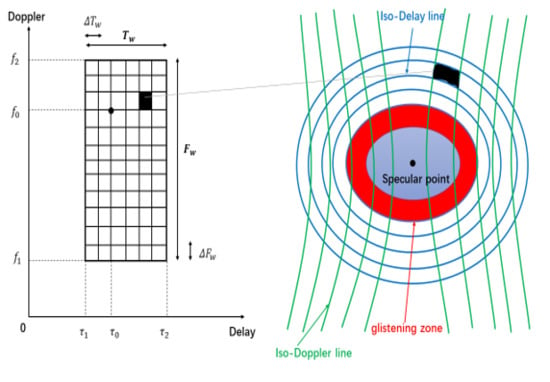
Due to the roughness of the land or sea surface, the signal received by the receiver is the energy reflected from the effective scattering area, including the scattering points. The scattering point is in the luminous region, and its size is related to sea surface roughness, receiver height, and elevation angle. In a light-emitting area, due to GNSS satellites and because the location of the receiver is constantly changing, each scattering point corresponds to a different Doppler frequency shift and Delay, respectively, to connect the same Delay and Doppler point from the Delay line (iso-Delay, nearly elliptic) and Doppler line (iso-Doppler, close to hyperbolic), and maps the light areas of each point to Doppler and Delay space and can get a Delay Doppler Map. GNSS signal is a kind of direct sequence spread spectrum signal, the satellite signal distribution within a wide frequency band, and, as a result of the limitation of the satellite launch power the space of long-distance transmission caused by the free space attenuation, and the existence of reflection, scattering the signal will leave high gain buried in noise, only through correlation processing to complete after capturing and tracking the measurement, as shown in Figure 1. Due to the reflection surface roughness, the reflection signals show the signal amplitude attenuation and different time Delay and Doppler signal superposition. The different delay and Doppler are opposite to the different reflection units of the reflection surface.

The reflection signal correlation value, therefore, needs, from two aspects of time delay and the Doppler frequency shift, the delay-Doppler correlation function ${\mathrm{Y}}_{R-Delay-Dop}\left(t_0,\tau ,f\right)$, see formula (1), and it reflects that the reflex zones at each time delay line and Doppler wire cross-area reflected signal correlation value are the most comprehensive description of the reflected signal.

$${\mathrm{Y}}_{R-Delay-Dop}\left(t_0,\tau ,f\right)={{\displaystyle \int }}_0^{T_i}{u}_R\left(t_0+t^{\prime }+\tau \right)a\left(t_0+t^{\prime }\right)exp\left[2\pi j\left(f_L+{\hat{f}}_R+f\right)\left(t_0+t^{\prime }\right)\right]d{t}^{\prime },$$

(1)

where, $T_i$ is the integration time, $u_R$ is the output signal receiving antenna, $a$ is the local pseudo random noise (PRN) code copy code, $f_L$ is the center of the received signal frequency, ${\hat{f}}_R$ is the reference point estimate Doppler. Each CYGNSS satellite had four DDMIs to observe four different highlights, so ideally CYGNSS could obtain 32 DDMs per second. The development of CYGNSS provided us with the first opportunity to estimate the global mean sea surface height (MSSH) based on the DDM obtained from the CYGNSS.

2.2. Specular Reflection Point Computation

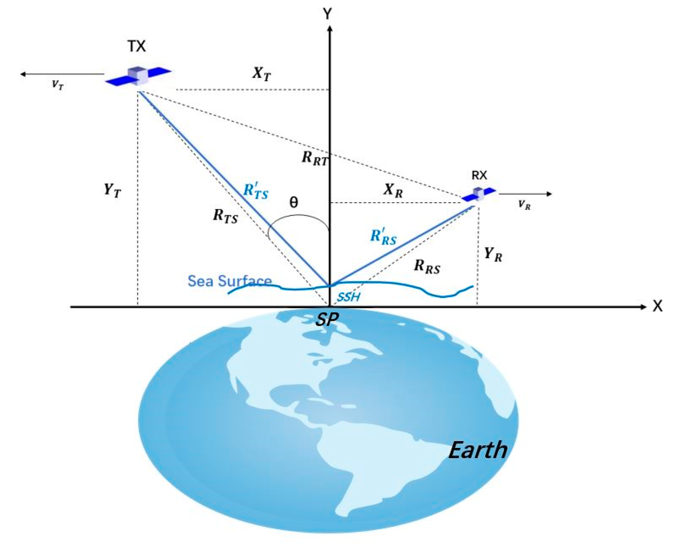
Sea surface height (SSH) is the height from sea level to the WGS84 ellipsoidal surface. As shown in Figure 2, the CYGNSS needs to find its reference point on the WGS84 ellipsoidal surface after receiving signals from the effective reflection area to further obtain the average sea surface height of the effective reflection area. In Figure 2, $RX$ is the receiver and $TX$ is the GNSS satellites, point $SP$ is the mirror reflection point, point $O$ is the center of the Earth, and $r$ is the radius of the Earth. The specular reflection point is on the Earth’s surface. Of all the points on the Earth’s surface, the distance from the transmitter to the point and then to the receiver is the shortest. The specular reflection point satisfies three conditions: (1) the specular reflection point is on the Earth’s surface; (2) the shortest path between the transmitter, receiver, and specular reflection point; (3) the incident angle at the specular reflection point is equal to the reflected angle. According to these conditions, the mirror reflection point position can be roughly estimated, and then based on the angle bisector variable step length correction of specular reflection point position, through iterative calculation of the precise positioning of the specular reflection, compared to Gleason’s [17] and Wu’s [18] method, it can be the results of high precision by the faster iteration [19].

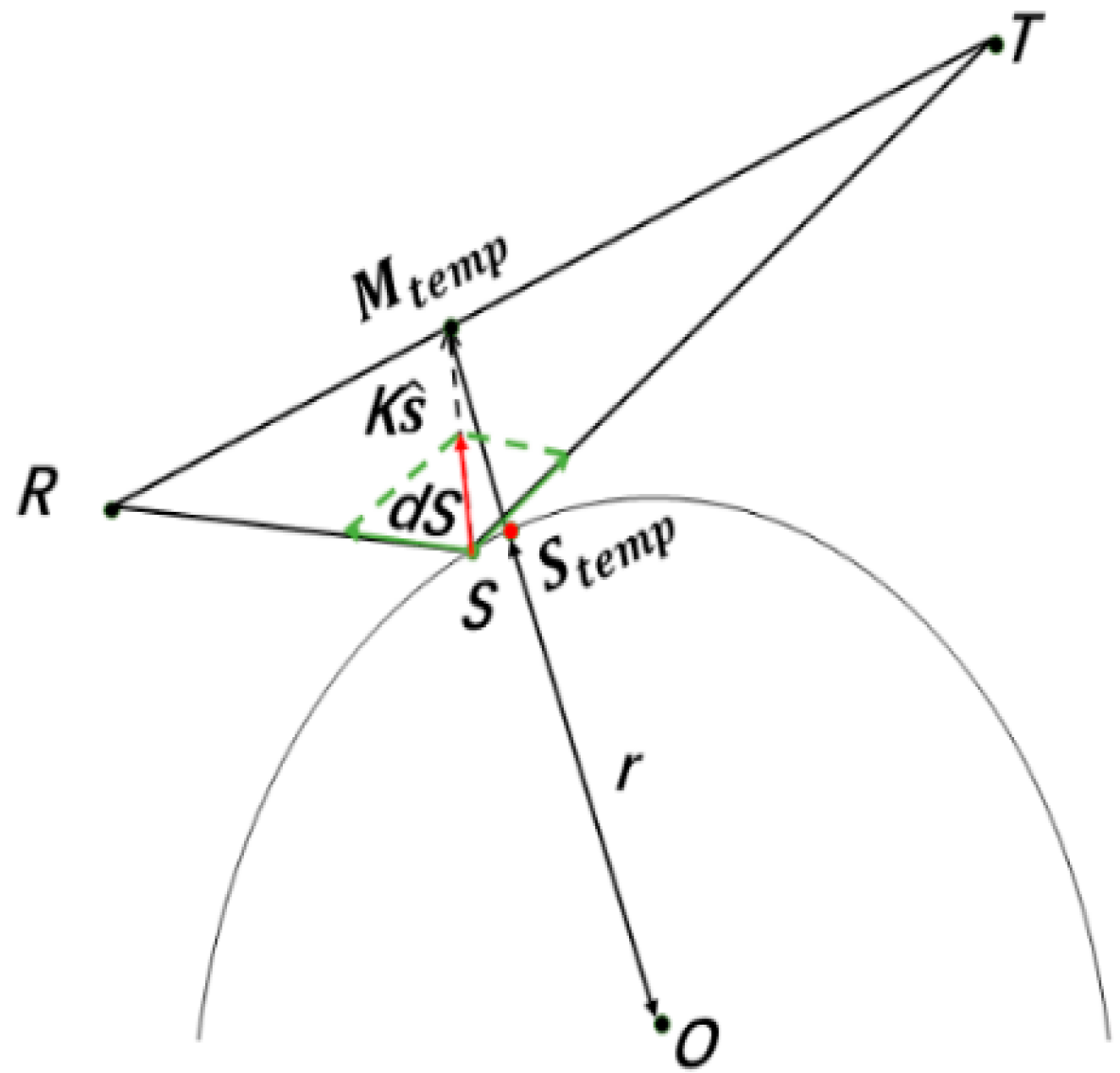
As shown in Figure 3, $R$ is the receiver, $T$ is the GNSS, point $S$ is the initial position of the specular reflection point, point $O$ is the center of the Earth, $r$ is the Earth’s radius, $\hat{s}$ is the correct direction, $K$ is correction step, $S_{temp}$ is a new mirror point location, based on the geometric relation in the diagram. We calculated the specular reflection point $S$ steps, which are as follows:

(1)

Enter the location of the receiver and transmitter obtained from the navigation information.

(2)

Using the formulas (2–5) roughly use $S$ as the initial position.

$$\overrightarrow{M} \approx \overrightarrow{R}+\frac{H_R}{H_R+H_T}\overrightarrow{RT},$$

(2)

$$\lambda ={\sin }^{-1} \frac{M_z}{\left|\overrightarrow{M}\right|},$$

(3)

$$r=a_{WGS84}\sqrt{\frac{1-e_{WGS84}^2}{1-\left(e_{WGS84}^2{\cos }^2\lambda \right)}},$$

(4)

$$\overrightarrow{S}=\frac{\overrightarrow{M}}{\left|\overrightarrow{M}\right|}r,$$

(5)

where, $H_R$ and $H_T$ are the heights of receiver and GNSS satellite, respectively. In the WGS84 coordinate system, the long radius $a_{WGS84}$ is 6,378,137 m and the eccentricity $e_{WGS84}$ is 0.081819190 84264.

(3)

Correct direction $\hat{s}$ calculated using Formulas (6) and (7).

$$d\overrightarrow{S}=\frac{\overrightarrow{ST}}{\left|\overrightarrow{TS}\right|}+\frac{\overrightarrow{SR}}{\left|\overrightarrow{RS}\right|},$$

(6)

$$\hat{s}=\frac{d\overrightarrow{S}}{\left|d\overrightarrow{S}\right|},$$

(7)

(4)

Correction step $K$ is calculated using Formula (8).

$$K=\sqrt{\left|TS\right|\left|RS\right|-\frac{{\left|TR\right|}^2\left|TS\right|\left|RS\right|}{{\left(\left|TS\right|+\left|RS\right|\right)}^2}},$$

(8)

(5)

Formulas (9) and (10) are used to calculate the new mirror point position $S_{temp}$.

$${\overrightarrow{M}}_{temp}=\overrightarrow{S}+K\hat{s},$$

(9)

$${\overrightarrow{S}}_{temp}=\frac{{\overrightarrow{M}}_{temp}}{\left|{\overrightarrow{M}}_{temp}\right|}r,$$

(10)

(6)

If conditions $\left|{\overrightarrow{S}}_{temp}-\overrightarrow{S}\right|<\epsilon$ is set up, then $\overrightarrow{S}$ is the final mirror reflection point, otherwise, let $\overrightarrow{S}={\overrightarrow{\mathrm{S}}}_{temp}$ and then go back to Step (3) to continue to iteration.

After calculating the position of the specular reflection point on the WGS84 ellipsoid, the time delay and Doppler frequency shift of the point can be calculated, which is the first step to calculate the mean sea surface height (MSSH).

2.3. Tracking Point Delay Estimation Method

The previous section introduced the estimation method of the WGS84 specular reflection point. In the actual measurement, to obtain the delay difference, it is necessary to estimate the delay of the actual reflection, which is the delay of the shortest path reflected to the sea surface. Cardellach et al. proposed three methods to obtain the actual delay [20], all of which were obtained based on the delay-related waveform, as follows:

(1)  First derivative spectrophotometry

This estimation method is to put the actual delay ${\tau }_{spec}$ as the solution of Equation (11).

$$\frac{d^{2}W}{d{\tau }^2}\left({\tau }_{spec}\right)=0,$$

(11)

In the equation, $W$ is delay relative waveforms (DM), which can be caused by the time delay Doppler figure (DDM). We can know that this point from the formula delays is the peaks of the wave’s first derivative.

(2)  Rule of Maximum Area

Another tracking point delay estimation method is based on the GNSS navigation time delay estimation method. In GNSS navigation, the time delay of the peak power is treated as the time delay of the navigation signal. When the surface is smooth, the algorithm only involves mirror delay, in which case, the tiny surface roughness does not affect the shape of the waveform. However, in Marine GNSS reflection measurement, the power waveform and peak are essentially determined by the roughness. Therefore, this method can be used in Global Navigation Satellite System-Reflectometry (GNSS-R) altimetry if the surface is smooth enough [21].

(3)  Half Peak Method

This algorithm is a simplified version of the algorithm used in single base radar altimetry. At the front edge of the waveform, the time delay corresponding to a part of the peak power is regarded as the actual time delay. In the altimetry measurement of the radar, the coefficient is very close to 0.5, which is the reason why the algorithm is named. In GNSS-R, this coefficient is generally selected as 0.75 because its result is very close to that of the first-order derivative method. It is important to note that when the coefficient is very close to 1, like the peak itself, it is strongly affected by the roughness of the ocean surface.

In order to reduce the inversion error of the actual Delay, the method by Mashburn et al. can be used to perform preliminary processing to improve the results. In other words, the interpolation processing of the DM can be performed using the Whitker–Shannon theorem [22], as shown in Formula (12).

$$X\left(\delta \right)={\displaystyle \sum }_{n=-\infty }^{\infty }x\left[n\right]\cdot sinc\left(\frac{\delta -nd}{d}\right),$$

(12)

where the $x\left[n\right]$ is related to the power sequence of the original time delay, $\delta$ is the extended time delay sequence, and $d$ is the sampling period. By comparing the three methods of actual time delay estimation, the influence of different inversion methods on the measurement accuracy is analyzed, and finally the first method is selected for the subsequent sea surface height calculation.

2.4. Sea Surface Height Calculation

After calculating the delay of the WGS84 specular reflection point and the actual delay, according to the geometric relationship in Figure 2, the sea surface height (SSH) of the effective reflection area can be calculated, according to Formulas (13–16) [23] proposed by Clarizia et al.

$$L=R_{TS}+R_{RS}-c\cdot \Delta \tau ,$$

(13)

$$\alpha =\frac{Y_R-Y_T}{L},$$

(14)

$$\beta =\frac{R_{TS}^2-R_{RS}^2+L^2}{2L},$$

(15)

$$SSH=\frac{-\left(\alpha \cdot \beta +Y_T\right)+\sqrt{{\left(\alpha \cdot \beta +Y_T\right)}^2-\left({\alpha }^2-1\right)\cdot \left({\beta }^2-R_{TS}^2\right)}}{{\alpha }^2-1},$$

(16)

Because the effective scattering area is very small, the sea level change in this very small area is also very small. This inversion method takes advantage of this feature and assumes that the longitude and latitude of the tracking points are the same as those of the WGS84 specular reflection points, thus reducing unknown variables to sea surface height (SSH) and achieving the goal of inversion sea surface height.

3. Results and Analysis

3.1. MSSH from CYGNSS

The mean sea surface height (MSSH) is the focus of current Earth science and environmental science. Compared with the reference ellipsoid, it contains the information of geoid and sea surface topography, so it is widely used to study geoids, instantaneous sea surface height, crustal deformation, ocean circulation, sea level change, and other issues. The global mean sea surface height model is obtained by using abundant satellite altimetry-measuring data (ERS-1, ERS-2, Jason series, etc.) and corresponding data processing. Generally, the model is based on grid data, which can be interpolated to obtain the sea surface height of a certain location in the world. The global mean sea surface height (MSSH) models used in this paper are CNES_CLS2015, provided by AVISO and DTU-10 models.

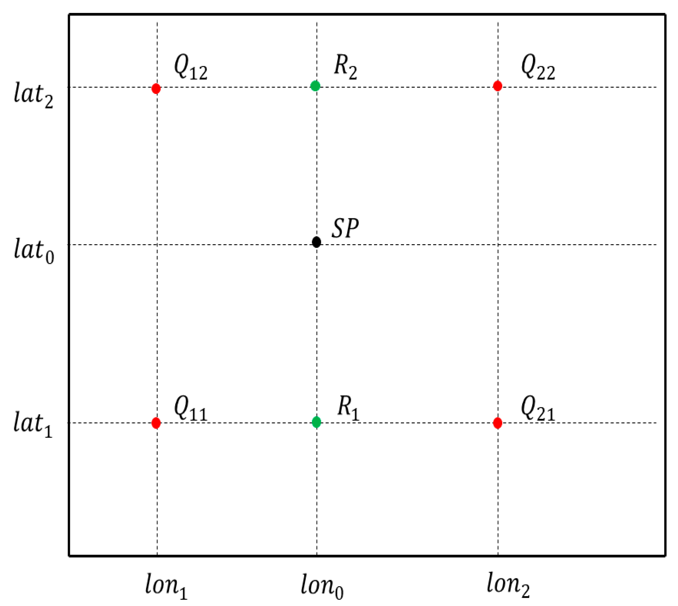
Since the resolution of the MSSH model is different from that of CYGNSS inversion, data matching is required for comparison. The bilinear interpolation method can be used to match two points. The $lo{n}_0$ and $la{t}_0$ are latitude and longitude, respectively, and the inversion results are $H_{measured}$. The position of this point on the MSSH grid is shown in Figure 4. According to Formulas (17–19), the $H_{measured}$ of the sea surface height of the $SP$ point in the MSSH grid can be calculated.

$$H_{R_1}=\frac{lo{n}_2-lo{n}_0}{lo{n}_2-lo{n}_1}{H}_{Q_{11}}+\frac{lo{n}_0-lo{n}_1}{lo{n}_2-lo{n}_1}{H}_{Q_{21}},$$

(17)

$$H_{R_2}=\frac{lo{n}_2-lo{n}_0}{lo{n}_2-lo{n}_1}{H}_{Q_{12}}+\frac{lo{n}_0-lo{n}_1}{lo{n}_2-lo{n}_1}{H}_{Q_{22}},$$

(18)

$$H_{model}=\frac{la{t}_2-la{t}_0}{la{t}_2-la{t}_1}{H}_{R_1}+\frac{la{t}_0-la{t}_1}{la{t}_2-la{t}_1}{H}_{R_2},$$

(19)

Among them, $H_{Q_{11}}$, $H_{Q_{21}},H_{Q_{12}},\mathrm{and}{H}_{Q_{22}}$ can be found in the MSSH model grid, according to $lo{n}_1,lo{n}_2,la{t}_1,\mathrm{and}la{t}_2$. After matching, a series of corresponding $lo{n}_0,la{t}_0$, $H_{measured}$, and $H_{model}$ can be evaluated. In this paper, the bias average absolute error (MAE), root mean square error (RMSE), and correlation coefficient (R) are calculated by using Formulas (20–23).

$$bias=H_{measured}^i-H_{model}^i,$$

(20)

$$MAE=\frac{1}{N}{{\displaystyle \sum }}_{i=1}^N\left|H_{measured}^i-H_{model}^i\right|,$$

(21)

$$RMSE=\sqrt{\frac{1}{N}{{\displaystyle \sum }}_{i=1}^N{\left(H_{measured}^i-H_{model}^i\right)}^2},$$

(22)

$$R=\frac{{{\displaystyle \sum }}_{i=1}^N\left(H_{measured}^i-{\overline{H}}_{measured}\right)\left(H_{model}^i-{\overline{H}}_{model}\right)}{\sqrt{{{\displaystyle \sum }}_{i=1}^N{\left(H_{measured}^i-{\overline{H}}_{measured}\right)}^2{{\displaystyle \sum }}_{i=1}^N{\left(H_{model}^i-{\overline{H}}_{model}\right)}^2}},$$

(23)

where, the ${\overline{H}}_{measured}$ is the average of $H_{measured}$, and the ${\overline{H}}_{model}$ is the average of $H_{model}$.

3.2. Comparison with AVISO

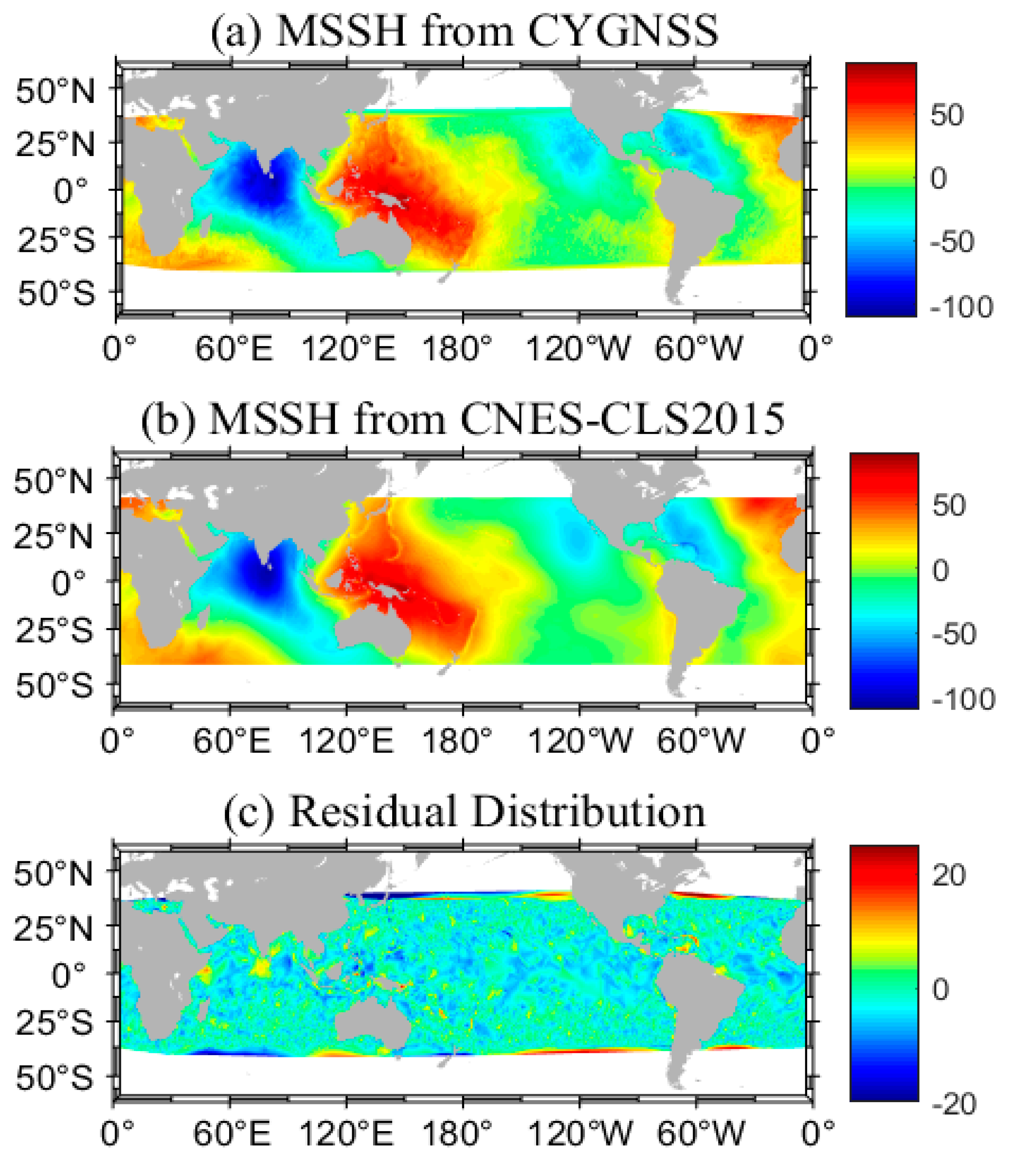
The first global mean sea surface height model used in this paper is CNES_CLS2015, provided by AVISO. The model uses 20 years (1993–2012) of altimetry data, mainly including Topex/Poseidon, ERS-2, GFO, Jason-1, Jason-2, Envisat, ERS-1, Jason-1, and Cryosat-2. The model currently offers a 1 min resolution global grid product available on the AVISO website. In addition to CNES_CLS2015, AVISO has previously released several related products, including CLS_SHOM98.2, CNES_CLS01, CNES_CLS10, and CNES_CLS2011. In this study, CYGNSS L1 was used in August 2017 to obtain the global mean sea surface height distribution, mainly including bistatic radar cross section (BRCS) data, spacecraft position, specular point position, GPS spacecraft position, and the incidence angle using the method in Section 2. We firstly used the position data named ‘tx_pos’ and ‘sc_pos’ to compute the position of the specular point on WGS84, according to the method in Section 2.2, and then we used the data named ‘sp_pos’, ‘sp_lat’, and ‘sp_lon’ to check our results. After the tested position was computed, we got the specular delay simply. In this experience, the spatial resolution was 0.1° $\times$ 0.1°, and each grid had about 30 measurements. The sea surface high monitoring area was the maximum range that the CYGNSS constellation could reach, including the full longitude range, and the latitude range was about 40° N~40° S. The average sea surface height distribution of the monitored sea areas obtained by the CNES_CLS2015 model is shown in Figure 5.

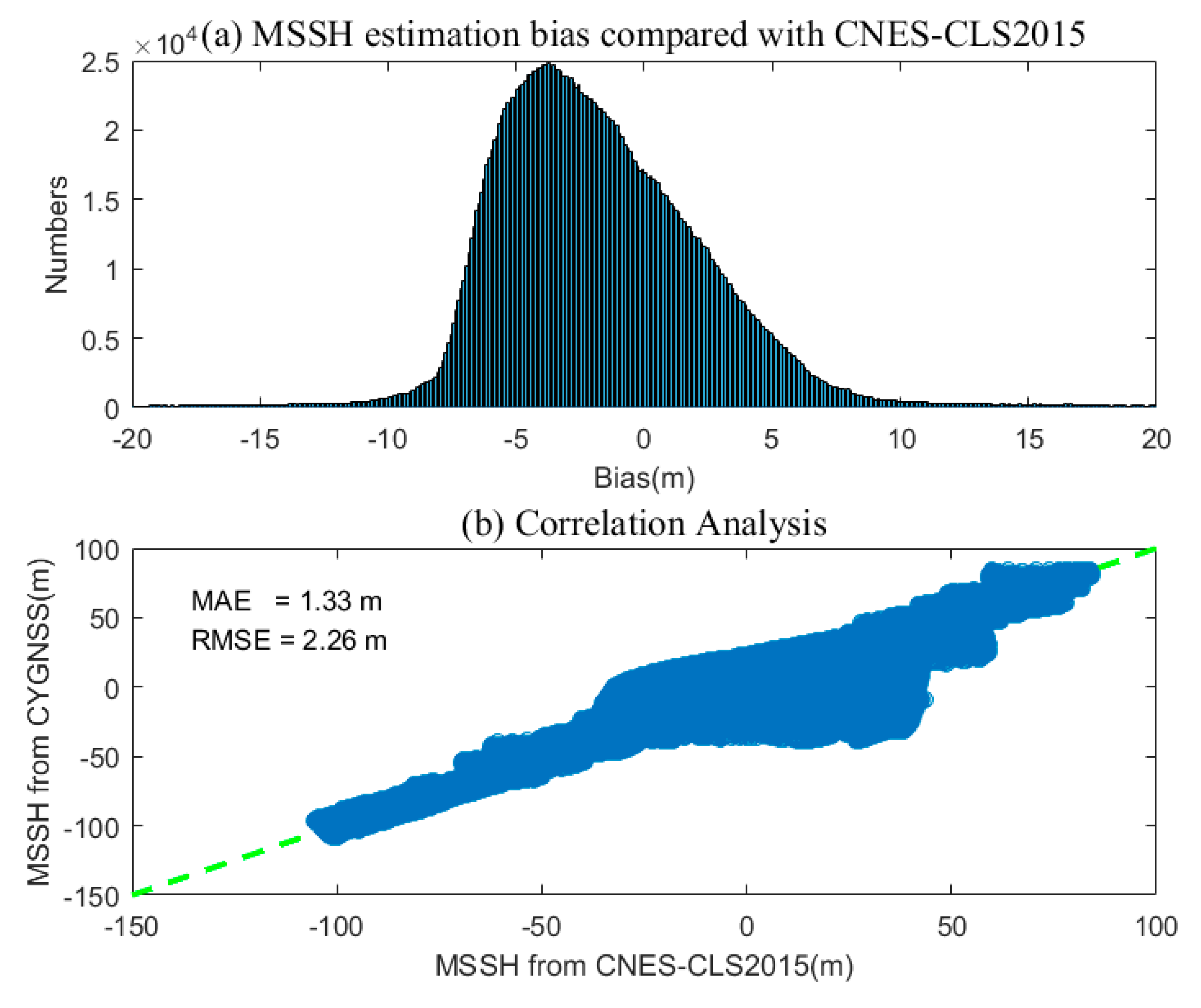
The inversion results were generally consistent with the CNES_CLS2015 model. The average sea surface height in the western Pacific is high and positive, which means that the average sea surface height here was higher than the WGS84 ellipsoid, and the average sea surface height in the Northern Indian Ocean is low and negative, which means that the average sea surface here was lower than the WGS84 ellipsoid. Considering Section 3.2, about the comparison of evaluation methods, as shown in Figure 6, you can see CYGNSS estimation results and CNES_CLS2015 model mainly concentrated in the deviation plus or minus 10 m and a small amount of distribution in the plus or minus 10 to 20 m. The graphics are very close to a Gaussian probability density distribution, and, at the same time, two set of values of the average absolute error was 1.33 m, root mean square error ($\mathrm{RMSE}$) was 2.26 m, and the correlation coefficient ($\mathrm{R}$) was 0.97, which is very similar in both groups. The results of the inversion results within a certain precision are credible.

3.3. Comparison with DTU-10

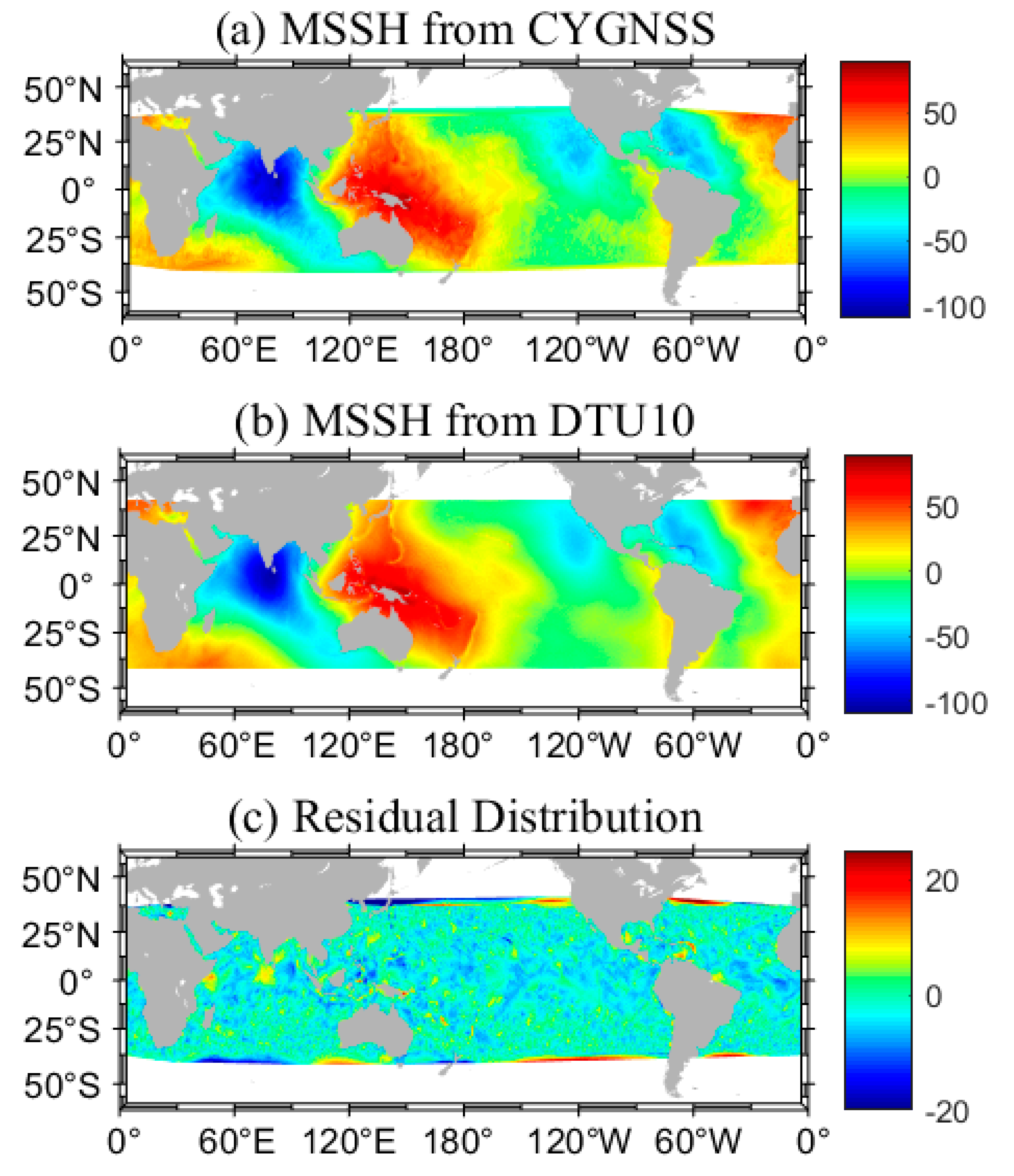
Another global mean sea surface height model used in this paper is DTU-10, which is the global mean sea surface height model proposed by Andersen et al., from Denmark Technical University in 2010, which is based on the DNSC08 model and improved. The DNSC08 model was also proposed by Andersen et al., which mainly used nine altimetry satellites, including Jason-1, T/P, T/P interleaved mission, ERS-1 GM, ERS-2 Exact Repeat Mission (ERM), Geosat GM, Geosat follow-on (GFO)-ERM, Envisat ERM, and ICESat, and 12 years of observation data were averaged. Compared with DNSC08, DTU-10 extended data coverage, averaged 17 years of data, and took ENVISAT data from ERS-2 and ENVISAT again. Dtu-10 data mainly include 1 min and 2 min resolution global grid products, and the specific products can be obtained from the official website of the DTU-10 server.

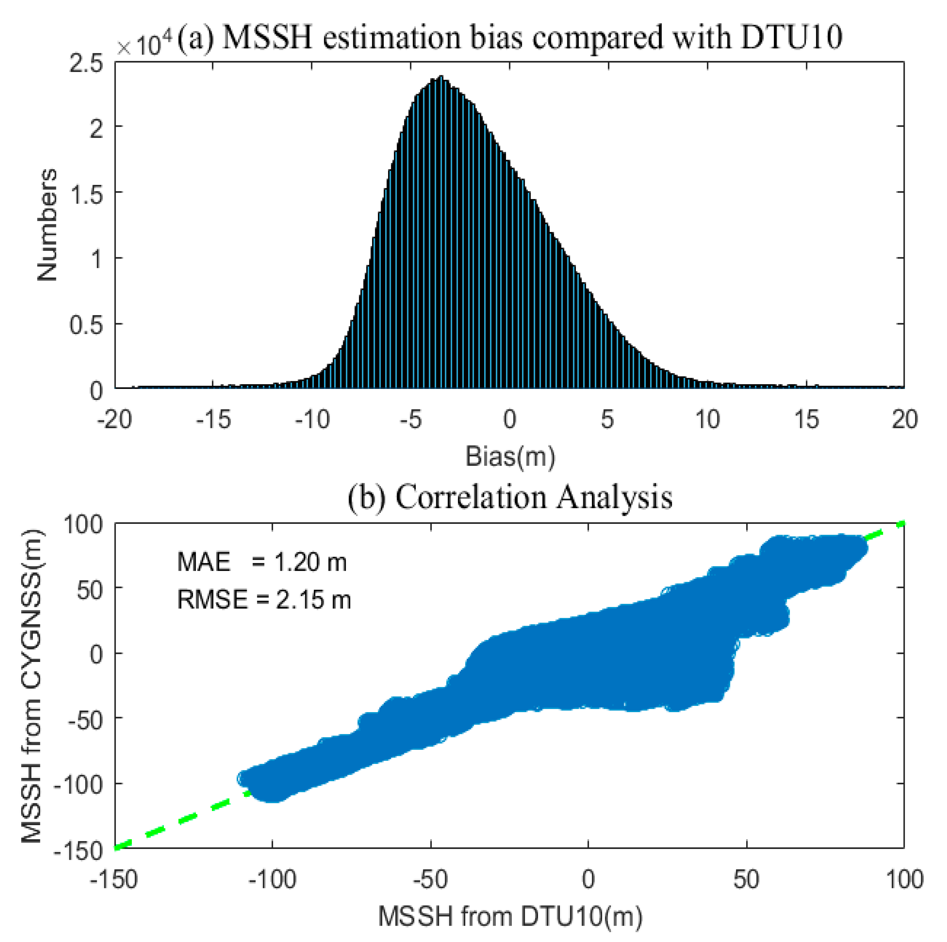
Similar to Section 3.2, Figure 7 and Figure 8 can be obtained. The sea surface height obtained through CYGNSS inversion is consistent with the value of the DTU10 model, because DTU10 model and CNSE_CLS2015 model have strong consistencies. It can be seen that the differences between CYGNSS results and the DTU10 model are mainly concentrated within 10 m and the distributions are very close to a Gaussian probability density distribution. The average absolute error was 1.20 m, the root mean square error ($\mathrm{RMSE}$) was 2.15 m, and the correlation coefficient ($\mathrm{R}$) was 0.97.

3.4. Comparison with Jason-2

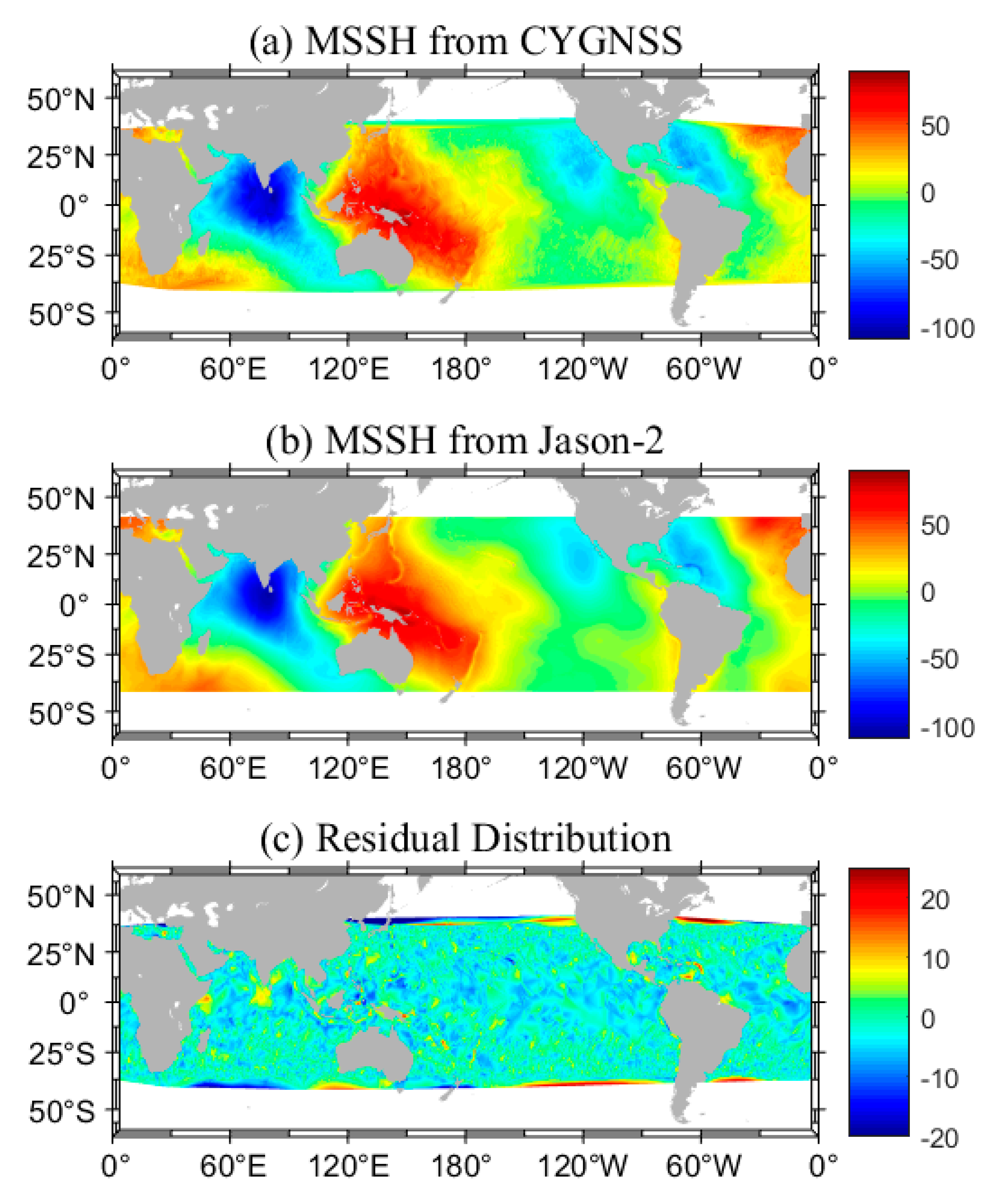
Jason-2/Ocean Surface Topography Mission (OSTM) took over and continued Topex/Poseidon and Jason-1 missions in 2008, in the frame of a cooperation between Center National d’Etudes Spatiales (CNES), Eumetsat, NASA and National Oceanic and Atmospheric Administration (NOAA). It carried two predecessors for a high-accuracy altimetry mission: a Poseidon-class altimeter, a radiometer, and three location systems. Its orbital inclination was 66° and the altitude was 1336 km. From 2008 to October 2016, Jason-2 was located on its nominal orbit. From October 2016 (at the end of cycle 303 and until cycle 327), after more than 8 years of service on this nominal ground track, Jason-2 swifted to the interleaved orbit. From July 2017 (beginning cycle 500), Jason-2 operated on a new long-repeat orbit (LRO) at roughly 1309.5 km altitude. From July 2018 (beginning cycle 600), Jason-2 operated on an interleaved long repeat orbit (i-LRO) for the second geodetic cycle, on a ground track in the middle of the grid defined by the first geodetic cycle. The sea surface height anomalies (SSHA) data can be download from AVISO, including the information of mean sea surface. The reference of Jason-2 is CLS01 MSS. Using Formula (24), SSH data can be calculated.

$$SSH=\overline{SSH}+SSHA,$$

(24)

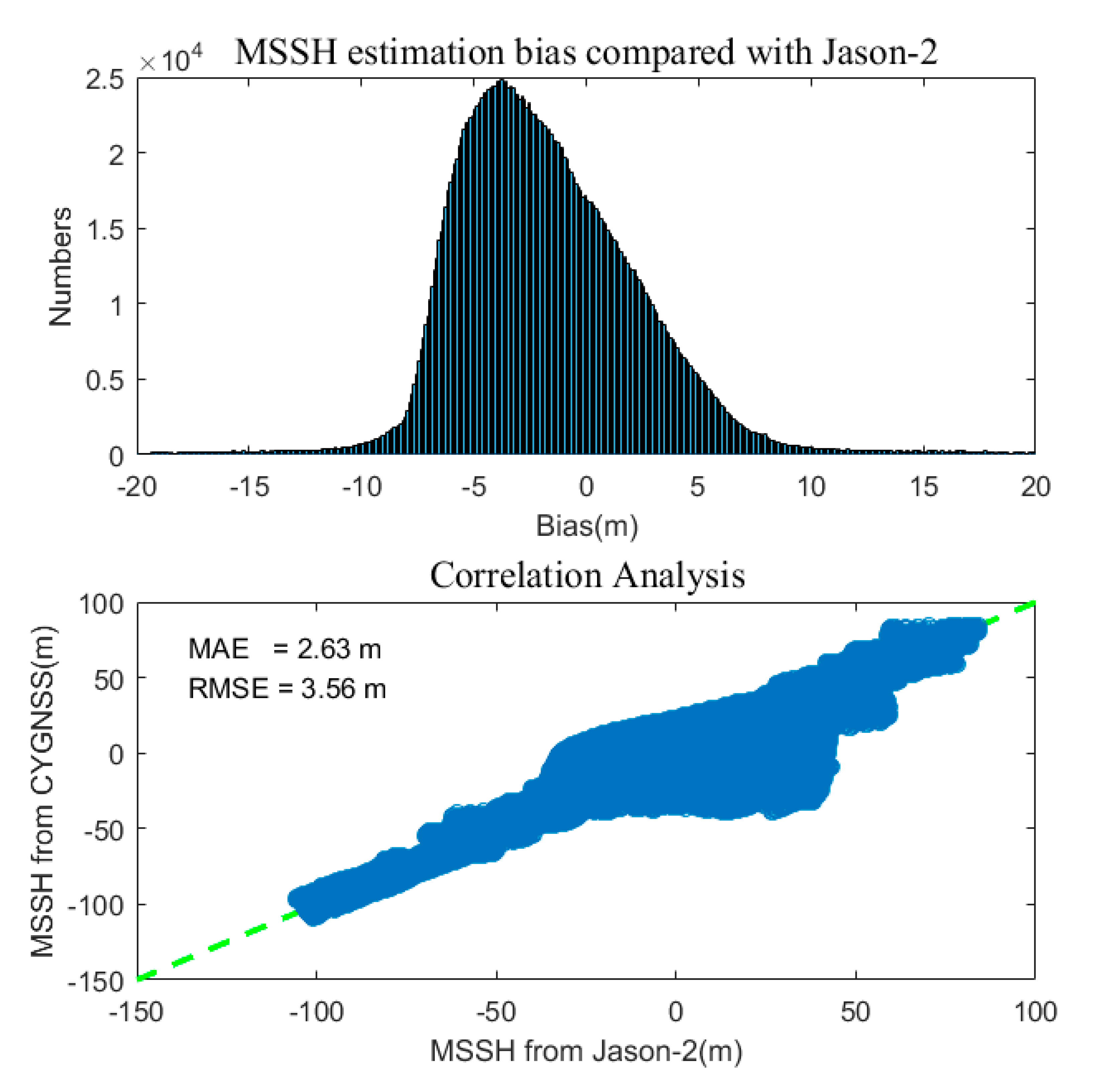
where, $\overline{SSH}$ is the reference that can be got from the data. Data for August 2017 were collected to calculate the mean sea surface and then compared with the CYGNSS result. Similar to Section 3.2 and Section 3.3, Figure 9 and Figure 10 can be obtained. The sea surface height obtained through CYGNSS inversion is consistent with the value of Jason-2′s results. It can be seen that the deviation of CYGNSS estimation results and Jason-2′s results were mainly concentrated in the plus or minus 10 m and a small amount of distribution in the plus or minus 10 to 20 m. The graphics were very close to a Gaussian probability density distribution, and, at the same time, two set of values of the average absolute error were 2.63 m, the root mean square error ($\mathrm{RMSE}$) was 3.56 m, the correlation coefficient ($\mathrm{R}$) was 0.95, that value was very similar in both groups. The results of inversion results within a certain precision are credible.

3.5. Errors Discussion

In the whole sea surface height inversion process, the biggest error comes from the inversion accuracy of the actual time delay, as shown in Figure 4. Formula (25) can be obtained from the geometric relationship.

$$c\cdot {\tau }_{spec}=R_{TS}^{\prime }+R_{RS}^{\prime }=\sqrt{{\left(R_{TS}\times \sin \theta \right)}^2+{\left(SSH-R_{TS}\times \cos \theta \right)}^2}+\sqrt{{\left(R_{RS}\times \sin \theta \right)}^2+{\left(SSH-R_{RS}\times \cos \theta \right)}^2},$$

(25)

Take the partial derivative and get Formula (26).

$$\frac{c\cdot d{\tau }_{spec}}{dSSH}=\frac{SSH-R_{TS}\times \cos \theta }{R_{TS}^{\prime }}+\frac{SSH-R_{RS}\times \cos \theta }{R_{RS}^{\prime }},$$

(26)

Due to $\mathrm{SSH}\ll R_{TS}^{\prime },R_{RS}^{\prime }$, $R_{TS}^{\prime }$≈$R_{TS}$, and $R_{RS}^{\prime }$≈ $R_{RS}$, Equation (26) can be simplified to Equation (27). The error of actual measurement delay directly affects the inversion of mean sea level height.

$$dSSH\approx -\frac{c\cdot d{\tau }_{spec}}{2\cos \theta },$$

(27)

Due to the delay of the CYGNSS resolution, which was about 0.255/1023000 s, according to Formula (27), it can be calculated for the lowest height inversion effect, which was about 37 m. When the incident angle was small, the time Delay error of height error was bigger, based on one dimensional time delay waveform figure (delay map) inversion when actual Delay. In order to reduce the actual inversion error of time delay, the Whitaker–Shannon theorem of DM interpolation processing can improve the result.

Except for the time delay estimation error and the receiver position, the GNSS position error was also bigger, because the location precision of the CYGNSS providing for level meters. This will bring the ideal mirror reflection point estimation error and can eventually bring the mean sea level height inversion error, which was about 3 m. Using the precise ephemeris and using appropriate methods to remove the ionosphere, troposphere, tidal, and pressure on the influence of orbit determination, this error was greatly reduced. Finally, the inherent errors of the instrument should also be considered. The noise of the instrument also affected the time delay, orbit determination, and ultimately the inversion of the mean sea level. With improvement of GNSS-R receivers and more spaceborne GNSS-R missions in the future, precise ocean environmental remote sensing will be expected from spaceborne GNSS-R observations [24,25,26,27,28].

4. Conclusions

In this paper, DDM data, provided by CYGNSS space-borne GNSS-R observations was used to invert the time delay of reflected signals according to the relation between peak position, half-peak position, and first-order derivative peak position of DM and the propagation time of reflected signals. In August 2017, the MSSH was obtained from CYGNSS data, which are validated by satellite altimetry CNES_CLS2015, DTU10 and Janson-2 results. The mean absolute error between the MSSH from the CYGNSS and the MSSH from the CNES_CLS2015 model was 1.33 m, the root mean square error was 2.26 m, and the correlation coefficient was 0.97. Compared with the DTU10 sea surface height model, the mean absolute error was 1.20 m, the root mean square error was 2.15 m, and the correlation coefficient was 0.97. Compared with Jason-2 results in August 2017, the mean absolute error was 2.63 m, the root mean square error was 3.56 m, and the correlation coefficient was 0.95. Therefore, the MSSH estimation from the CYGNSS can provide important support for marine shipping development, marine environmental protection, marine disaster warnings, and forecasting, etc. Here, the precision was global, and the performance in each grid will be further investigated in the future.

The CYGNSS MSSH estimation method requires high spatial resolution, and the time required for the grid to produce high-precision data is also long, so the time resolution of the obtained estimation value is low. Furthermore, the influence of other satellite parameters, such as the satellite orbital error, should be analyzed in the future in order to reduce these effects. Due to the covering limitation of the CYGNSS observation area, the CYGNSS can only estimate the MSSH of the area within 40 degrees north and south latitude. In addition, the estimation of MSSH based on the CYGNSS just considered one single parameter. In the future, multi-parameters, such as sea surface wind speed and significant wave height, are brought into the MSSH estimation, which may improve the accuracy of the MSSH estimation.

References

- Dong, X.; Huang, C. Monitoring Global Mean Sea Level Variation with TOPEX/Poseidon Altimetry. Acta Geod. Cartogr. Sin. 2000, 29, 266–272. [Google Scholar]
- Jin, T.; Li, J.; Jiang, W. The global mean sea surface model WHU2013. Geod. Geodyn. 2016, 7, 202–209. [Google Scholar] [CrossRef] [Green Version]
- Jin, S.G.; Qian, X.D.; Wu, X. Sea level change from BeiDou Navigation Satellite System-Reflectometry (BDS-R): First results and evaluation. Glob. Planet. Chang. 2017, 149, 20–25. [Google Scholar] [CrossRef]
- Martineira, M. A passive reflectometry and interferometry system (PARIS): Application to ocean altimetry. ESA J. 1993, 17, 331–355. [Google Scholar]
- Barrick, D.E. Rough Surface Scattering Based on the Specular Point Theory. IEEE Trans. Antennas Propag. 1968, 16, 449. [Google Scholar] [CrossRef]
- Garrison, J.L.; Katzberg, S.J. The application of reflected GPS signals to ocean remote sensing. Remote Sens. Environ. 2000, 73, 175–187. [Google Scholar] [CrossRef]
- Elfouhaily, T.; Thompson, D.R.; Linstrom, L. Delay-Doppler analysis of bistatically reflected signals from the ocean surface: Theory and application. IEEE Trans. Geosci. Remote Sens. 2002, 40, 560–573. [Google Scholar] [CrossRef]
- Rius, A.; Aparicio, J.M.; Cardellach, E.; Martin-Neira, M.; Chapron, B. Sea surface state measured using GPS reflected signals. Geophys. Res. Lett. 2002, 29, 37. [Google Scholar] [CrossRef] [Green Version]
- Addabbo, P.; Giangregorio, G.; Galdi, C.; Di Bisceglie, M. Simulation of TechDemoSat-1 delay-Doppler maps for GPS ocean reflectometry. IEEE J. Sel. Top. Appl. Earth Obs. Remote Sens. 2017, 10, 4256–4268. [Google Scholar] [CrossRef]
- Yang, D.K.; Zhang, Q.S.; Zhang, Y.Q.; Hu, R.L. Design and realization of Delay Mapping Receiver based on GPS for sea surface wind measurement. In 2006 1st IEEE Conference on Industrial Electronics and Applications; IEEE: New York, NY, USA, 2006; Volume 1–3, p. 149. [Google Scholar]
- Li, W.Q.; Cardellach, E.; Fabra, F.; Rius, A.; Ribo, S.; Martin-Neira, M. First spaceborne phase altimetry over sea ice using TechDemoSat-1 GNSS-R signals. Geophys. Res. Lett. 2017, 44, 8369–8376. [Google Scholar] [CrossRef]
- Foti, G.; Gommenginger, C.; Jales, P.; Unwin, M.; Shaw, A.; Robertson, C.; Rosello, J. Spaceborne GNSS reflectometry for ocean winds: First results from the UK TechDemoSat-1 mission. Geophys. Res. Lett. 2015, 42, 5435–5441. [Google Scholar] [CrossRef] [Green Version]
- Soulat, F.; Caparrini, M.; Germain, O.; Lopez-Dekker, P.; Taani, M.; Ruffini, G. Sea state monitoring using coastal GNSS-R. Geophys. Res. Lett. 2004, 31, 4. [Google Scholar] [CrossRef] [Green Version]
- Awada, A.; Khenchaf, A.; Coatanhay, A. Bistatic radar scattering from an ocean surface at L-band. In Proceedings of the 2006 IEEE Radar Conference, Verona, NY, USA, 24–27 April 2006; Volume 1–2, p. 200. [Google Scholar]
- Li, W.; Cardellach, E.; Fabra, F.; Ribó, S.; Rius, A. Assessment of Spaceborne GNSS-R Ocean Altimetry Performance Using CYGNSS Mission Raw Data. IEEE Trans. Geosci. Remote Sens. 2019, 58, 238–250. [Google Scholar] [CrossRef]
- Zuffada, C.; Li, Z.J.; Nghiem, S.V.; Lowe, S.; Shah, R.; Clarizia, M.P.; Cardellach, E. The Rise of Gnss Reflectometry for Earth Remote Sensing. In Proceedings of the 2015 IEEE International Geoscience and Remote Sensing Symposium, Milan, Italy, 26–31 July 2015; pp. 5111–5114. [Google Scholar]
- Gleason, S.T.; Hodgart, S.; Sun, Y.; Gommenginger, C.; Mackin, S.; Adjrad, M.; Unwin, M. Detection and Processing of bistatically reflected GPS signals from low Earth orbit for the purpose of ocean remote sensing. IEEE Trans. Geosci. Remote Sens. 2005, 43, 1229–1241. [Google Scholar] [CrossRef] [Green Version]
- Wu, S.C.; Meehan, T.; Young, L. The potential use of GPS signals as ocean altimetry observables. In Proceedings of the National Technical Meeting—Navigation and Positioning in the Information Age, Santa Monica, CA, USA, 14 January 1997; pp. 543–550. [Google Scholar]
- Yuan, H.U.; Wang, Y.J.; Liu, W.; Zi-Heng, Y.U. Specular Reflection Point Estimation for Global Navigation Satellite System Reflectometry Remote Sensing. Sci. Technol. Eng. 2018, 18, 108–113. [Google Scholar]
- Cardellach, E.; Rius, A.; Martin-Neira, M.; Fabra, F.; Nogues-Correig, O.; Ribo, S.; Kainulainen, J.; Camps, A.; D’Addio, S. Consolidating the Precision of Interferometric GNSS-R Ocean Altimetry Using Airborne Experimental Data. IEEE Trans. Geosci. Remote Sens. 2014, 52, 4992–5004. [Google Scholar] [CrossRef]
- Li, W.Q.; Cardellach, E.; Fabra, F.; Ribo, S.; Rius, A. Lake Level and Surface Topography Measured With Spaceborne GNSS-Reflectometry from CYGNSS Mission: Example for the Lake Qinghai. Geophys. Res. Lett. 2018, 45, 13332–13341. [Google Scholar] [CrossRef]
- Mashburn, J.; Axelrad, P.; Lowe, S.T.; Larson, K.M. Global Ocean Altimetry with GNSS Reflections from TechDemoSat-1. IEEE Trans. Geosci. Remote Sens. 2018, 56, 4088–4097. [Google Scholar] [CrossRef]
- Clarizia, M.P.; Ruf, C.; Cipollini, P.; Zuffada, C. First spaceborne observation of sea surface height using GPS-Reflectometry. Geophys. Res. Lett. 2016, 43, 767–774. [Google Scholar] [CrossRef] [Green Version]
- JIn, S.G.; Zhang, Q.; Zhang, X. New Progress and Application Prospects of Global Navigation Satellite System Reflectometry (GNSS + R). Acta Geod. Cartogr. Sin. 2017, 46, 1389–1398. [Google Scholar] [CrossRef]
- Peng, Q.; Jin, S.G. Significant Wave Height Estimation from Space-Borne Cyclone-GNSS Reflectometry. Remote Sens. 2019, 11, 584. [Google Scholar] [CrossRef] [Green Version]
- Jin, S.; Feng, G.P.; Gleason, S. Remote sensing using GNSS signals: Current status and future directions. Adv. Space Res. 2011, 47, 1645–1653. [Google Scholar] [CrossRef]
- Dong, Z.; Jin, S. Evaluation of Spaceborne GNSS-R Retrieved Ocean Surface Wind Speed with Multiple Datasets. Remote Sens. 2019, 11, 2747. [Google Scholar] [CrossRef] [Green Version]
- Jin, S.G.; Cardellach, E.; Xie, F. GNSS Remote Sensing: Theory, Methods and Applications; Springer: Amsterdam, The Netherlands, 2014; p. 276. [Google Scholar]
Figure 1.
The relationship between the delay-Doppler unit and the reflector unit.
Figure 2.
Reflectometry altimetry geometry.
Figure 3.
Specular reflection point search based on angular bisector.
Figure 4.
Bilinear interpolation schematic.
Figure 5.
(a) Global mean sea surface elevation map estimated by the Cyclone Global Navigation Satellite System (CYGNSS); (b) using the CNES_CLS2015 model to obtain the average sea surface height distribution of monitored sea areas; (c) the distribution of residual between (a,b).
Figure 6.
(a) Statistical chart of deviation between CYGNSS results and CNES-CLS2015 model values; (b) correlation analysis diagram of the CNES_CLS2015 model value and CYGNSS results.
Figure 7.
(a) Global mean sea surface height estimated by CYGNSS; (b) global mean sea surface height obtained by DTU10 model; (c) the residual between CYGNSS and DTU10.
Figure 8.
(a) The distribution of mean sea surface height (MSSH) differences between CYGNSS and the DTU10 model; (b) correlation and RMSE of the DTU10 model and CYGNSS results.
Figure 9.
(a) Global mean sea surface height estimated by CYGNSS; (b) global mean sea surface height obtained by the DTU10 model; (c) the residual between CYGNSS and DTU10.
Figure 10.
(a) The distribution of MSSH differences between CYGNSS and Jason-2; (b) correlation and RMSE of the DTU10 model and CYGNSS results.
© 2020 by the authors. Licensee MDPI, Basel, Switzerland. This article is an open access article distributed under the terms and conditions of the Creative Commons Attribution (CC BY) license (http://creativecommons.org/licenses/by/4.0/).
Share and Cite
MDPI and ACS Style
Qiu, H.; Jin, S. Global Mean Sea Surface Height Estimated from Spaceborne Cyclone-GNSS Reflectometry. Remote Sens. 2020, 12, 356. https://doi.org/10.3390/rs12030356
AMA Style
Qiu H, Jin S. Global Mean Sea Surface Height Estimated from Spaceborne Cyclone-GNSS Reflectometry. Remote Sensing. 2020; 12(3):356. https://doi.org/10.3390/rs12030356
Chicago/Turabian StyleQiu, Hui, and Shuanggen Jin. 2020. "Global Mean Sea Surface Height Estimated from Spaceborne Cyclone-GNSS Reflectometry" Remote Sensing 12, no. 3: 356. https://doi.org/10.3390/rs12030356
Note that from the first issue of 2016, this journal uses article numbers instead of page numbers. See further details here.