Improved SRGAN for Remote Sensing Image Super-Resolution Across Locations and Sensors

Abstract

Detailed and accurate information on the spatial variation of land cover and land use is a critical component of local ecology and environmental research. For these tasks, high spatial resolution images are required. Considering the trade-off between high spatial and high temporal resolution in remote sensing images, many learning-based models (e.g., Convolutional neural network, sparse coding, Bayesian network) have been established to improve the spatial resolution of coarse images in both the computer vision and remote sensing fields. However, data for training and testing in these learning-based methods are usually limited to a certain location and specific sensor, resulting in the limited ability to generalize the model across locations and sensors. Recently, generative adversarial nets (GANs), a new learning model from the deep learning field, show many advantages for capturing high-dimensional nonlinear features over large samples. In this study, we test whether the GAN method can improve the generalization ability across locations and sensors with some modification to accomplish the idea “training once, apply to everywhere and different sensors” for remote sensing images. This work is based on super-resolution generative adversarial nets (SRGANs), where we modify the loss function and the structure of the network of SRGANs and propose the improved SRGAN (ISRGAN), which makes model training more stable and enhances the generalization ability across locations and sensors. In the experiment, the training and testing data were collected from two sensors (Landsat 8 OLI and Chinese GF 1) from different locations (Guangdong and Xinjiang in China). For the cross-location test, the model was trained in Guangdong with the Chinese GF 1 (8 m) data to be tested with the GF 1 data in Xinjiang. For the cross-sensor test, the same model training in Guangdong with GF 1 was tested in Landsat 8 OLI images in Xinjiang. The proposed method was compared with the neighbor-embedding (NE) method, the sparse representation method (SCSR), and the SRGAN. The peak signal-to-noise ratio (PSNR) and structural similarity (SSIM) were chosen for the quantitive assessment. The results showed that the ISRGAN is superior to the NE (PSNR: 30.999, SSIM: 0.944) and SCSR (PSNR: 29.423, SSIM: 0.876) methods, and the SRGAN (PSNR: 31.378, SSIM: 0.952), with the PSNR = 35.816 and SSIM = 0.988 in the cross-location test. A similar result was seen in the cross-sensor test. The ISRGAN had the best result (PSNR: 38.092, SSIM: 0.988) compared to the NE (PSNR: 35.000, SSIM: 0.982) and SCSR (PSNR: 33.639, SSIM: 0.965) methods, and the SRGAN (PSNR: 32.820, SSIM: 0.949). Meanwhile, we also tested the accuracy improvement for land cover classification before and after super-resolution by the ISRGAN. The results show that the accuracy of land cover classification after super-resolution was significantly improved, in particular, the impervious surface class (the road and buildings with high-resolution texture) improved by 15%.

1. Introduction

Detailed and accurate information on the spatial variation of land cover and land use is a critical component of local ecology and environmental research. For these tasks, high spatial resolution images are required to capture the temporal and spatial dynamics of the earth’s surface processes [1]. Considering the trade-off between high spatial and high temporal resolution in remote sensing images, at present, there are two main methods for obtaining high spatio-temporal resolution images: 1) the multi-source image fusion models [2,3] and 2) the image super-resolution models [4,5].

Compared to the image fusion models, the methods in the super-resolution field do not require auxiliary high spatial resolution data with the same location and a similar observation date to predict the detailed spatial texture, which makes these methods more approachable for different scenarios in both the computer vision and remote sensing fields.

The basic assumption of the image super-resolution model is that missing details in a low spatial resolution image can be either reconstructed or learned from other high spatial resolution images if these images follow the same resampling process as was used to create the low spatial resolution image. Based on this assumption, in the last decade, efforts have been made to focus on accurately predicting the point spread function (PSF), which represents the mixture process that forms the low-resolution pixels. There are mainly three groups of methods: 1) interpolation-based methods, 2) refactoring-based methods, and 3) learning-based methods (

Table 1. The comparison of super-resolution methods.

Types of Method	Basic Hypothesis	Representative Models	Advantages	Disadvantage
Interpolation-based methods	The value of the current pixel can be represented by the nearby pixels	The nearest neighbor interpolation [6]	low complexity and high efficiency	No image texture detail can be predicted and usually makes the image smoother looking
		The bilinear interpolation [7]
		The bicubic interpolation [8]
Refactoring-based methods	The physical properties and features can be recovered by image reconstruction (RE) technology, and these rules of the point spread function (PSF) can be further applying for the detail recovering	Joint MAP registration [9]	The different information on the same scene is fused to obtain high-quality reconstruction results	Requires pre-registration and a large amount of calculation
		Sparse regression and natural image prior [11]
		Kernel regression
		PSF deconvolution [23]
Learning-based methods	The point spread function can be created by learning from a large number of image samples [24]	Neighbor-embedding (NE) [21]	Getting better performance when training samples are more like the target image, and can achieve a higher PSNR when a large number of samples are involved	Highly time consuming, requiring big training datasets and usually limited model generalization ability across datasets
		Convolutional neural network (SRCNN) [25]
		Bayesian networks [26]
		Kernel-based methods [27]
		SVM-based methods [28]
		Sparse representation (SCSR) [22]
		Super-resolution GAN(SRGAN) [29]

).

Firstly, the interpolation-based methods [6,7,8] are based on a certain mathematical strategy to calculate the pixel value of the target point to be restored from the relevant points, which is of low complexity and high efficiency. However, the edge effect in the resulting image is obvious, and the image details cannot be recovered since there is no new information produced in the interpolation process.

Secondly, the refactoring-based methods [9,10,11] model the imaging process and integrate different information from the same scene to obtain high-quality reconstruction results. Usually, these methods trade time differences for spatial resolution improvement, which usually requires pre-registration and a large amount of calculation.

Thirdly, the learning-based methods [12,13,14,15,16,17,18,19,20] overcome the limitation of the difficulty by determining the resolution improvement multiple of the reconstruction method and can be oriented towards a single image, which is the main development direction of the current super-resolution reconstruction. In this category, commonly used methods include the neighbor-embedding method (NE) [21], the sparse representation method (SCSR) [22] and the deep learning method.

The learning-based method usually requires the high representative of the training samples to cover the data variation of the whole population. In practice, a large number of training samples from different sources are usually collected to achieve this goal. However, in the remote sensing field, it is almost impossible to prepare such a training sample set because the variation of remote sensing data not only depends on the variation of the object but also on the different locations and different satellite sensors. Due to this limitation, many learning-based methods are limited to a certain location and specific sensor, resulting in the limited generalization ability of the model across locations and sensors. This limitation remains a challenge for producing one super-resolution model for different locations and different satellite sensors.

In recent years, with the rapid development of artificial intelligence, especially neural network-based deep learning methods, deep learning has been widely applied in the field of computer vision, due to its obvious advantages for nonlinear process fittings of large samples. One benefit of these models is their ability to handle large sample sets while retaining a good generalization ability. In the field of image super-resolution, the super-resolution CNN model (SRCNN) was first presented by Dong [25] in 2014. Compared with traditional image super-resolution, this method achieves a higher peak signal-to-noise ratio, but when the image on the sampling ratio is high, the reconstructed image will be too smooth, and details will be lost. To overcome this shortage, a super-resolution generative adversarial network model (SRGAN) was presented by replacing the original CNN structure with the generative adversarial network (GAN) [29]. As the newest learning model from the deep learning field, the SRGAN shows many advantages for capturing high-dimensional nonlinear features over large samples. However, the generalization ability of the SRGAN model in remote sensing images across different locations and sensors remains unknown.

In this study, we test whether the GAN-based method can improve the generalization ability across locations and sensors by making some modifications so that we can train once and apply the results everywhere and with different sensors. Our work is based on the SRGAN model by modifying the loss function and the structure of the network of the SRGAN. The major contributions of this study are as follows:

• We propose the improved SRGAN (ISRGAN), which stabilizes the model training and enhances the generalization ability across locations and sensors;
• We test the performance of the ISRGAN from two sensors (Landsat 8 OLI and Chinese GF 1) at different locations (Guangdong and Xinjiang in China). Specifically, for the cross-location test, the model training in Guangdong with the Chinese GF 1 data was tested with the GF 1 data in Xinjiang. For the cross-sensor test, the same model training in Guangdong with GF 1 was tested with the Landsat 8 OLI data in Xinjiang;
• The proposed method is compared to the neighbor-embedding (NE), sparse representation (SCSR), and the original SRGAN methods, and the results show that the ISRGAN achieved the best performance;
• The model provided in this study shows a good generalization ability across locations and sensors. This model can be further applied to other satellite sensors and different locations for image super-resolution to achieve the goal of “training once, apply to everywhere and different sensors.”

The structure of this paper is as follows: The overall workflow (Section 2.1), the review of the original SRGAN (Section 2.2), the problem of the original SRGAN and the corresponding improvement (Section 2.3) are described in the Methods section (Section 2). The study area, dataset and assessment method in this study are explained in the Experiments section (Section 3). Section 4 describes the main results and findings in our study. In Section 5, we discuss the advantages and possible further works followed by the Conclusion section (Section 6).

2. Methods

2.1. Workflow

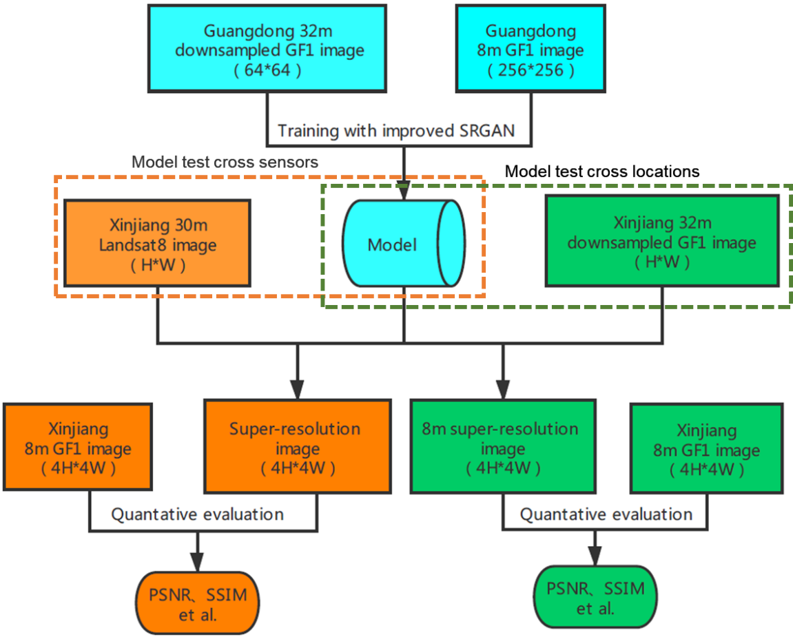
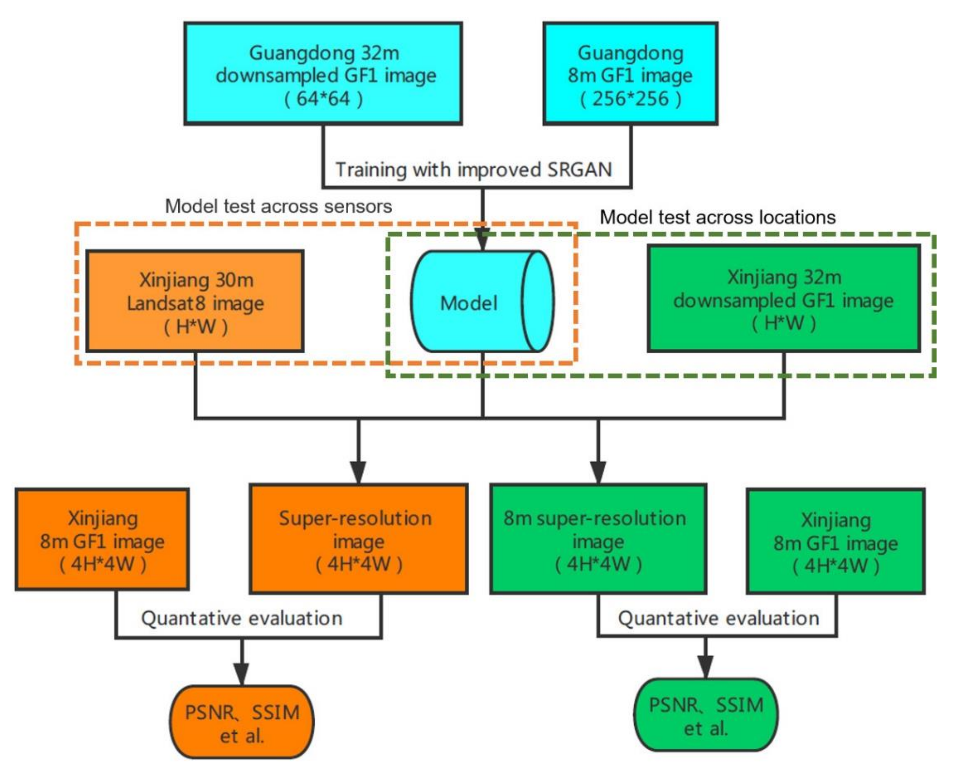
In this paper, the experiment on whether the super-resolution model has generalization capability across locations and sensors is mainly divided into three parts, as presented in Figure 1. The blue part represents the model training part, which used the GF 1 data in Guangdong. The green part indicates that the model was tested for generalization ability across regions, using the GF 1 data in Xinjiang. The orange part indicates that the model was tested for whether there was generalization ability across sensors, mainly using the Landsat 8 data in Xinjiang.

First, we used the ISRGAN to train the Guangdong GF 1 data and obtained the super-resolution model. At the same time, we divided the test set into three parts, namely test dataset 1 (GF 1 data in Guangdong province), test dataset 2 (GF 1 data in Xinjiang province) and test dataset 3 (Landsat 8 data in Xinjiang province).

For the test of whether the model had generalization ability across locations in the green part, we tested dataset 1 and dataset 2 and obtained the PSNR and SSIM, respectively, in order to conduct a t-test to determine whether the model had generalization ability across locations. For the test of whether the model had generalization ability across sensors in the orange part, we tested dataset 2 and dataset 3 and obtained the PSNR and SSIM, respectively, in order to conduct a t-test to determine whether the model had generalization ability across sensors.

2.2. SRGAN Review

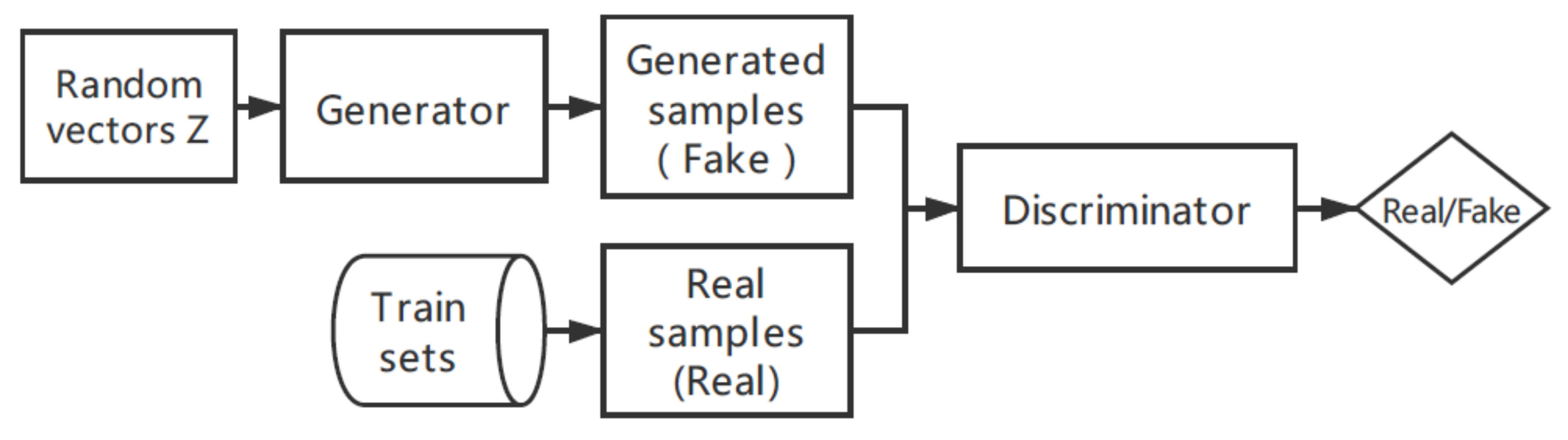
The GAN is a deep learning model proposed by Goodfellow et al. [30] in 2014. The structure of the GAN is inspired by the two-person zero-sum game in game theory. The framework consists of a generator (G) and a discriminator (D), where the generator (G) learns the distribution of real sample data and generates new sample data, and the discriminator (D) is a binary classifier used to distinguish whether the data is from real samples or generated samples. The structure diagram of the GAN is shown in Figure 2. The optimization process of the GAN is a minimax problem. When the generator and discriminator reach the Nash equilibrium, the optimization process is completed.

In machine learning, GANs have become a hot research direction. At present, the field of computer vision has become the most widely studied and applied field of GANs, which have broad applications.

The SRGAN is a super-resolution network structure proposed by Christian Ledig [29] in a paper published at the 2017 CVPR conference, which brings the effect of super-resolution to a new height. The SRGAN is trained based on the GAN network, which consists of a generator and a discriminator. The generators use a ResNet structure [31], the former part of the network is connected with several residual blocks, each containing two 3 × 3 convolution layers, which is followed by the batch normalization layer, which is activated with the ReLu function. In the latter part, two subpixel network modules are added to increase the size so that the generator can learn high-resolution image details in the front layer during the training process and improve the image resolution later, so as to achieve the purpose of reducing computing resources. The discriminator adopts the vgg-19 network structure [32], including eight convolution layers, where the LeakyReLu function is used as the activation function for the hidden layer, and finally, the probability of the predicted image coming from the real high-resolution and generated high-resolution image is obtained by using the full connection layer and sigmoid activation function.

The main innovation of the SRGAN is to propose an optimization algorithm of perceived loss based on a neural network, which is to replace the mean square error (MSE) content loss with the loss calculated based on the vgg-19 network feature map. The original pixel-level MSE loss calculation ($L_{mse}^{SR}$) and the characteristic loss calculation ($L_{VGG/i,j}^{SR}$) based on the vgg-19 network are shown in Equations (1) and (2), respectively

$$L_{mse}^{SR}=\frac{1}{r^{2}WH}{\displaystyle \sum }_{x=1}^{rW}{\displaystyle \sum }_{y=1}^{rH}{(I_{x,y}^{HR}-G_{\theta G}{(I^{LR})}_{x,y})}^2$$

(1)

$$L_{VGG/i,j}^{SR}=\frac{1}{W_{i,j}{H}_{i,j}}{\displaystyle \sum }_{x=1}^{W_{i,j}}{\displaystyle \sum }_{y=1}^{H_{i,j}}{({\varnothing }_{i,j}{(I^{HR})}_{x,y}-{\varnothing }_{i,j}{(G_{\theta G}(I^{LR}))}_{x,y})}^2$$

(2)

where represents the ratio between the spatial resolution of a high- and low-resolution image, W and H respectively represent the pixel numbers of the width and height of the low-resolution image, $W_{i,j}$ and $H_{i,j}$ represent the dimension of the corresponding feature map in the vgg-19 network, ${\varnothing }_{i,j}$ represents the feature map obtained before the $j^{th}$ convolution before the $i^{th}$ max-pooling layer within the vgg-19 network, $I{ }_{x,y}$ represents the gray value of the layer map at the point (x, y), and $G_{\theta G}$ represents the reconstructed image.

2.3. The Improved SRGAN

2.3.1. Problems in SRGAN

Due to the phenomena of gradient disappearance and mode collapse in the SRGAN training process, the model does not have a good generalization ability for remote sensing image super-resolution across locations and sensors. Next, we analyze the nature of this phenomenon.

The first phenomenon, gradient disappearance, can be explained as follows:

In the training process of the SRGAN, we want the discriminator to be strong enough to distinguish the samples well, and we want to give a result of 1 for the real high-resolution sample image and a result of 0 for the generated high-resolution sample image. Therefore, the discriminator loss function of the original SRGAN is shown in Equation (3):

$$maxV\left(G,D\right)=E_{x~P_r}\left[logD\left(HR\right)\right]+E_{x~P_g}\left[log\left(1-D\left(G\left(LR\right)\right)\right)\right]$$

(3)

where $V\left(G,D\right)$ represents the difference between the ground true high-resolution (HR) image and the model-generated image, HR and LR represent high-resolution images and low-resolution images, respectively, G and D represent the generator and discriminator, respectively, $P_r$ and $P_g$ represent the distribution of the real HR image and the generated super-resolution (SR) image, and E represents the expectation.

The generator hopes that the image generated by itself can be marked as 1 by the discriminator, so the adversarial loss function of the generator is:

$$minV\left(G,D\right)=E_{x~P_g}\left[log\left(1-D\left(G\left(LR\right)\right)\right)\right]$$

(4)

Therefore, the loss function of the SRGAN is shown in Equation (5):

$${}_G{}^{min} {}_D{}^{max}V\left(G,D\right)=E_{x~P_r}\left[logD\left(HR\right)\right]+E_{x~P_g}\left[log\left(1-D\left(G\left(LR\right)\right)\right)\right]$$

(5)

The training process of the SRGAN is divided into two steps. The first step is to fix the generator and train the discriminator. For Equation (3):

$$\begin{array}{cc}V\left(G,D\right)\hfill & =E_{x~P_r}\left[logD\left(HR\right)\right]+E_{x~P_g}\left[log\left(1-D\left(G\left(LR\right)\right)\right)\right]\hfill \\ \hfill & ={{\displaystyle \int }}_{HR}^{}{P}_{r}log\left(D\left(HR\right)\right)d\left(HR\right)+{{\displaystyle \int }}_{LR}^{}{P}_{g}log(1-D\left(G\left(LR\right)\right))d\left(LR\right)\hfill \\ \hfill & ={{\displaystyle \int }}_{HR}^{}(P_r\log \left(D\left(HR\right)\right)+P_{g}log(1\hfill \\ \hfill & -D\left(HR\right)))d\left(HR\right)\hfill \end{array}$$

(6)

In order to optimize the discriminator’s ability to distinguish data sources, Equation (6) is maximized as follows

$$D_G^{*}=\frac{P_r}{P_r+P_g}$$

(7)

where $D_G^{*}$ is the optimal discriminator.

The second step is to fix the discriminator trained in the first step to optimize the generator. For Equation (5), we substitute Equation (7) into it. The new form of $V\left(G,D\right)$ as shown in Equation (8):

$$\begin{array}{cc}V\left(G,D\right)\hfill & =E_{x~P_r}\left[log{D}_G^{*}\left(HR\right)\right]+E_{x~P_g}\left[log\left(1-D_G^{*}\left(G\left(LR\right)\right)\right)\right]\hfill \\ \hfill & =E_{x~P_r}\left[log\frac{P_r}{P_r+P_g}\right]+E_{x~P_g}\left[log\frac{P_g}{P_r+P_g}\right]\hfill \\ \hfill & ={{\displaystyle \int }}_{HR}^{}{P}_{r}log\frac{P_r}{P_r+P_g}d\left(HR\right)+{{\displaystyle \int }}_{LR}^{}{P}_{g}log\frac{P_g}{P_r+P_g}d\left(LR\right)\hfill \\ \hfill & =-2log2+{{\displaystyle \int }}_{HR}^{}{P}_{r}log\frac{P_r}{\frac{P_r+P_g}{2}}d\left(HR\right)+{{\displaystyle \int }}_{LR}^{}{P}_{g}log\frac{P_g}{\frac{P_r+P_g}{2}}d\left(LR\right)\hfill \end{array}$$

(8)

In addition, the Kullback-Leibler (KL) divergence and Jensen-Shannon Divergence (JSD) can be expressed as Equations (9) and (10)

$$KL(P_1||P_2)=E_{x~P_1}log\frac{P_1}{P_2}=\int P_{1}log\frac{P_1}{P_2}dx$$

(9)

$$JSD(P_1||P_2)=\frac{1}{2}(KL(P_1||\frac{P_1+P_2}{2})+KL(P_1||\frac{P_1+P_2}{2}))$$

(10)

where $P_1$ and $P_2$ represent the two probability distributions.

By substituting Equations (9) and (10) into Equation (8), we can get the final form of $V\left(G,D\right)$

$$\begin{gathered} V\left(G,D\right)=-2log2+KL(P_r||\frac{P_r+P_g}{2})+KL(P_g||\frac{P_r+P_g}{2}) \\ =-2log2+2JSD(P_r||P_g) \end{gathered}$$

(11)

where $JSD(P_r||P_g)$ represents the JSD divergence of the $P_r$ and $P_g$.

As can be seen from Equation (11), only if $P_r=P_g$, V(G, D) reaches the minimum value is the generation effect the best. In practice, the generated distribution can only be infinitely close to the real distribution, but the two can never overlap completely. According to Equation (11), only when the real distribution and the generated distribution overlap completely is the $V\left(G,D\right)$ equal to $-2log2$, otherwise, it always equals 0. Therefore, when using the gradient descent method, the generator cannot get any gradient information, which means it faces the problem of gradient disappearance.

The second phenomenon, mode collapse, can be explained as follows:

The generator loss function can also be written as:

$$E_{x~P_g}\left[-\log \left(D\left(G\left(LR\right)\right)\right)\right]$$

(12)

Due to the KL divergence, $P_r$ and $P_g$ can be transformed into the form containing D*:

$$\begin{gathered} KL(P_g||P_r)=E_{x~P_g}\left[log\frac{P_g}{P_r}\right]=E_{x~P_g}\left[log\frac{\frac{P_g}{P_g+P_r}}{\frac{P_r}{P_g+P_r}}\right]=E_{x~P_g}\left[log\frac{1-D_G^{*}}{D_G^{*}}\right] \\ =E_{x~P_g}\log \left[1-D_G^{*}\right]-E_{x~P_g}log{D}_G^{*} \end{gathered}$$

(13)

From Equations (12) and (13), it can be concluded that the loss function is equivalent to:

$$\begin{gathered} E_{x~P_g}\left[-\log \left(D_G^{*}\left(G\left(LR\right)\right)\right)\right]=KL(P_g||P_r)-E_{x~P_g}\log \left[1-D_G^{*}\left(G\left(LR\right)\right)\right] \\ =KL(P_g||P_r)-2JS(P_r||P_r)+2log2+E_{x~P_r}log{D}_G^{*}\left(HR\right) \end{gathered}$$

(14)

Since only the first two terms depend on the generator (G), the final loss function of the generator is equivalent to minimizing the following function:

$$F=KL(P_r||P_g)-2JS(P_r||P_g)$$

(15)

According to Equation (15), in the process of training the discriminator, the KL divergence should be reduced while the JS divergence should be increased, resulting in unstable training. At the same time, due to the asymmetry of the KL divergence, the following phenomenon occurs: the generator generates an unreal image, and the punishment is relatively high, so the generator generates an image similar to the real image, with a lower penalty. The result of this phenomenon is that the generator tends to produce similar images, which is called the mode collapse problem.

The two problems stated above led to the unstable performance of the SRGAN in the training process, which led to a poor generalization ability for remote sensing image super-resolution across locations and sensors.

2.3.2. Improved SRGAN

Inspired by the idea of WGANs [33], we modified the loss function and the partial structure of the network in view of the weak generalization ability caused by the instability of the SRGAN in the training process and proposed the ISRGAN. In this paper, the Wasserstein distance is used to replace the KL divergence and JS divergence. The calculation of the Wasserstein distance is shown in Equation (16)

$$V\left(G,D\right)=W\left(P_r,P_g\right)=\begin{array}{c}inf\\ \gamma ~\prod (P_r,P_g)\end{array}{E}_{\left(x,y\right)~\gamma }\left[\left|\left|x-y\right|\right|\right]$$

(16)

where $W\left(P_r,P_g\right)$ represents the Wasserstein distance of the $P_r$ and $P_g$, $\gamma$ represents the joint distribution of the real HR image and the generated image, $\prod (P_r,P_g)$ represents the set of all possible joint probability distributions of the $P_r$ and $P_g$, $\left|\left|x-y\right|\right|$ represents the distance between a pair of samples x and y, $\left(x,y\right)~\gamma$ represents how much “mass” must be transported from x to y in order to transform the distributions of the $P_r$ into the distribution of the $P_g$, and the marginal distributions of x and y are the $P_r$ and $P_g$, respectively, and inf represents the lower bound that we can take on the expectation of all possible joint distributions.

However, when learning the image distribution, the random variable has thousands of dimensions, and it is difficult to solve directly by solving the linear programming problem. Therefore, we convert it into the dual form

$$V\left(G,D\right)=W\left(P_r,P_g\right)=\frac{1}{K}\begin{array}{c}sup\\ |\left|f\right|{|}_L\le K\end{array}{E}_{x~P_r}\left[f\left(x\right)\right]-E_{x~P_g}\left[f\left(x\right)\right]$$

(17)

where $|\left|f\right|{|}_L\le K$ means that f is a K-Lipschitz function, the K-Lipschitz function is defined as, for K >0, $\left|\left|f\left(x_1\right)-f\left(x_2\right)\right|\left|\le K\right|\left|x_1-x_2\right|\right|$ and K is the Lipschitz constant of $f$, and sup represents the upper bound of the expectation. Therefore, based on the SRGAN structure and the ideal of the WGAN, this paper modifies the network structure, and the loss function during training can be summarized as follows:

(1)

Sigmoid was removed from the last layer of the discriminator to transform the classification problem into a regression problem;

(2)

The loss functions of the generator and discriminator were not logarithmic;

(3)

During the training process, after updating the discriminator parameters, its absolute value was truncated to no more than a fixed constant;

(4)

The convolution kernel of the last layer of the generator was changed from 1 × 1 to 9 × 9.

3. Experiments

3.1. Study Area

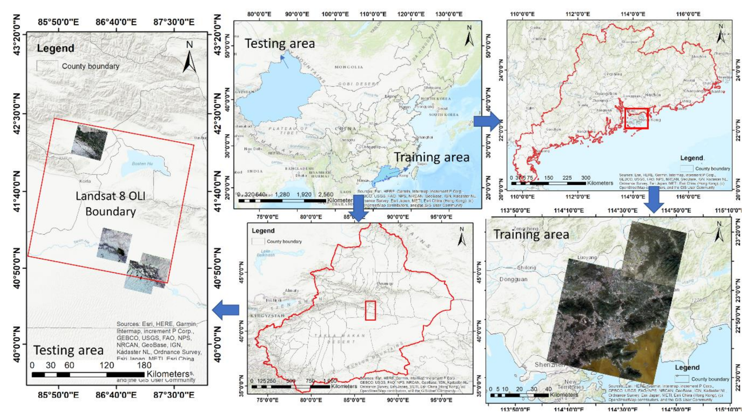
The study area selected included some areas of the Guangdong–Hong Kong–Macao greater bay area and Yuli county, Xinjiang. The Guangdong–Hong Kong-–Macao greater bay area is located in the pearl river delta of Guangdong, which is the fourth largest bay area in the world after the New York bay area, the San Francisco bay area, and the Tokyo bay area. The economic foundation of this region is solid, the development potential is huge, and it has a pivotal status; Yuli county, located in the middle of Xinjiang, is an important transportation hub in Xinjiang. The area is particularly rich in mineral resources and tourist resources and is known as the “back garden” of Korla. The two research areas are representative of the study of the super-resolution of remote sensing images and subsequent ground-object extraction. Figure 3 shows the image coverage of GF 1 in the study area.

3.2. Data and Datasets

The experimental data included the GF 1 satellite data (Land observation satellite data service platform: http://218.247.138.119:7777/DSSPlatform/index.html) and the Landsat 8 satellite data (the USGS Earth Explorer: https://earthexplorer.usgs.gov/). The GF 1 satellite was successfully launched from the Jiuquan Satellite Launch Center on April 26, 2013, and is the first satellite from a major Chinese project using a high-resolution earth observation system. The GF 1 satellite is equipped with two 2-m panchromatic resolution cameras, two 8-m resolution multispectral cameras, and four 16-m resolution multispectral wide-width cameras, among which PMS sensor multispectral cameras contain four bands: blue, green, red, and near-infrared. Landsat 8 was launched by NASA on February 11, 2013, and is equipped with two sensors: the Operational Land Imager (OLI) and the Thermal Infrared Sensor (TIRS) thermal infrared sensor, among which the OLI sensor multispectral cameras contain nine bands: coastal, blue (B), green (G), red (R), near-infrared (NIR), short wave infrared 1 (SWIR1), and short wave infrared 2 (SWIR2). The details are shown in

Table 2. The parameters of GF 1.

Parameters	2m-PAN Sensor/8m-MS Sensor		16m-MS Sensor
Spectral range	Panchromatic	0.45-0.90um
	Multispectral	0.45-0.52um	0.45-0.52um
		0.52-0.59um	0.52-0.59um
		0.63-0.69um	0.63-0.69um
		0.77-0.89um	0.77-0.89um
Spatial resolution	Panchromatic	2m	16m
	Multispectral	8m
Scale range	60km (2 cameras)		800km (4 cameras)
Revisit cycle (side swing)	4 days
Revisit cycle (non-side swing)	41 days		4 days

and

Table 3. The parameters of Landsat 8.

Sensor	Band	Spectral Range/um	Spatial Resolution/m
OLI	1-COASTAL	0.43-0.45	30
	2-Blue	0.45-0.51	30
	3-Green	0.53-0.59	30
	4-Red	0.64-0.67	30
	5-NIR	0.85-0.88	30
	6-SWIR1	1.57-1.65	30
	7-SWIR2	2.11-2.29	30
	8-PAN	0.50-0.68	15
	9-Cirrus	1.36-1.38	30
TIRS	10-TIR	10.60-11.19	100
	11-TIR	11.50-12.51	100

.

Table 4. The information of used data.

Location	Sensor	Latitude and Longitude	Time	Filename
Guangdong	GF1-PMS1	E114.2, N22.7	20171211	GF1_PMS1_E114.2_N22.7_20171211_L1A0002840075
Guangdong	GF1-PMS1	E114.3, N23.0	20171211	GF1_PMS1_E114.3_N23.0_20171211_L1A0002840076
Guangdong	GF1-PMS2	E114.6, N22.7	20171211	GF1_PMS2_E114.6_N22.7_20171211_L1A0002840310
Guangdong	GF1-PMS2	E114.6, N22.9	20171211	GF1_PMS2_E114.6_N22.9_20171211_L1A0002840309
Guangdong	GF1-PMS2	E114.7, N23.2	20171211	GF1_PMS2_E114.7_N23.2_20171211_L1A0002840307
Xinjiang	GF1-PMS1	E86.3, N42.2	20180901	GF1_PMS1_E86.3_N42.2_20180901_L1A0003427463
Xinjiang	GF1-PMS1	E86.6, N41.1	20171028	GF1_PMS1_E86.6_N41.1_20171028_L1A0002715402
Xinjiang	GF1-PMS1	E87.2, N40.8	20171130	GF1_PMS1_E87.2_N40.8_20171130_L1A0002807153
Xinjiang	GF1-PMS2	E87.0, N40.7	20170917	GF1_PMS2_E87.0_N40.7_20170917_L1A0002605364
Xinjiang	Landsat-8 OLI	E86.2, N41.7	20171229	LC08_L1TP_143031_20171229_20180103_01_T1

shows the data details used in this paper. Considering the difference in the spectral range between the two kinds of satellite data in each channel, the experimental data selected in this paper only includes three RGB bands.

When doing the experiment, we need to make sure that the same ratio of the high-resolution image and low-resolution image pixel must be strictly 1:4, while the GF 1 PMS sensor data and Landsat satellite’s OLI sensor data is not a strict 1:4 relation. In order to guarantee the feasibility of the experiment, we used the GF1 data and cut it into images of 256 × 256 size, while obtaining images of 64 × 64 size through cubic subsampling. Finally, we selected 3200 images of 256 × 256 size and their subsamples for training as high-resolution and low-resolution images, respectively.

3.3. Network Parameter Setting and Training

The proportion factor of the high-resolution image (HR) and low-resolution image (LR) used in the experiment was × 4, among which the LR images were obtained by sampling the HR image four times, using the nearest-neighbor method in Python. During training, the batch size was set to 16, and the training process was divided into two steps. In the first step, the ResNet [31] was trained to obtain the mean square error (MSE) between the generated high-resolution image and the real high-resolution image, namely the traditional pixel-based loss, and the learning rate was initialized to 10^-4, training 100 epochs in total. In the second step, we used the model trained in the first step as the initialization of the generator. Using pretreatment based on pixel losses can make the method based on the GAN achieve a better effect. The reason for this can be summarized as follows: 1) The high-resolution image generated by preprocessing is a relatively good image for the discriminator, so it pays more attention to texture details in the following training process. 2) It is better to avoid the generator reaching the local optimization. The initialization learning rate of the generator training was 10^-4, and it was reduced to 1/2 in each 250 iterations, training 500 epochs in total.

We used the RMSProp optimization algorithm to update the generator and discriminator alternately until the model converged. The model was implemented using the Tensorflow framework (Google Inc. https://www.tensorflow.org) and was trained on four NVIDIA GeForce GTX TITAN X GPUs. The code is modified based on the SRGAN code, which can be freely downloaded from the GitHub website (https://github.com/tensorlayer/srgan).

3.4. Assessment

In this paper, we adopted the peak signal-to-noise ratio (PSNR) [34] and structural similarity index measurement (SSIM) [35] as the evaluation indexes for the experimental results. Usually, after an image is compressed, the image spectrum will change, so the output image will be somewhat different from the original image. In order to measure the quality of the processed image, the PSNR is usually used to measure whether a processor meets the expected requirements and is calculated as follows

$$PSNR=10\times lo{g}_{10}\left(\frac{MA{X}^2}{MSE}\right)$$

(18)

where the MSE is calculated as shown in Equation (19)

$$MSE=\frac{{{\displaystyle \sum }}_{n=1}^N\left(I^n-P^n\right)}{N}$$

(19)

where $I^n$ refers to the gray value of the $n^{th}$ pixel of the original image, and $P^n$ refers to the gray value of the $n^{th}$ pixel after processing. The unit of the peak signal-to-noise ratio (PSNR) is dB, and the higher the value, the better the image quality.

SSIM is a method used to measure the subjective experience quality of television, film, or other digital images and video. This method was first proposed by the image and video engineering laboratory of the University of Texas at Austin and then developed in cooperation with New York University. The SSIM algorithm is used to test the similarity of two images, and its measurement or prediction of image quality is based on uncompressed or undistorted images as a reference. The model measures image similarity in brightness, contrast, and structure. Its calculation is shown in Equation (20)

$$SSIM\left(X,Y\right)=\frac{\left(2u_X{u}_Y+C_1\right)\left(2{\sigma }_{XY}+C_2\right)}{\left(u_X^2+u_Y^2+C_1\right)\left({\delta }_X^2+{\delta }_Y^2+C_2\right)}$$

(20)

where $u_X$ and $u_Y$ represent the means of the gray values of image X and image Y, respectively, and ${\delta }_X^2$, ${\delta }_Y^2$ and ${\sigma }_{XY}$ represent the variances of the gray values of image X and image Y, respectively.

Generally, $C_1={(K_1*L)}^2,C_2={(K_2*L)}^2,K_1=0.01,K_2=0.03$ and L is the maximum image value. The range of SSIM is (0,1); the larger its value, the less image distortion there is.

4. Results

4.1. High Spatial Resolution Image of ISRGAN across Locations and Sensors

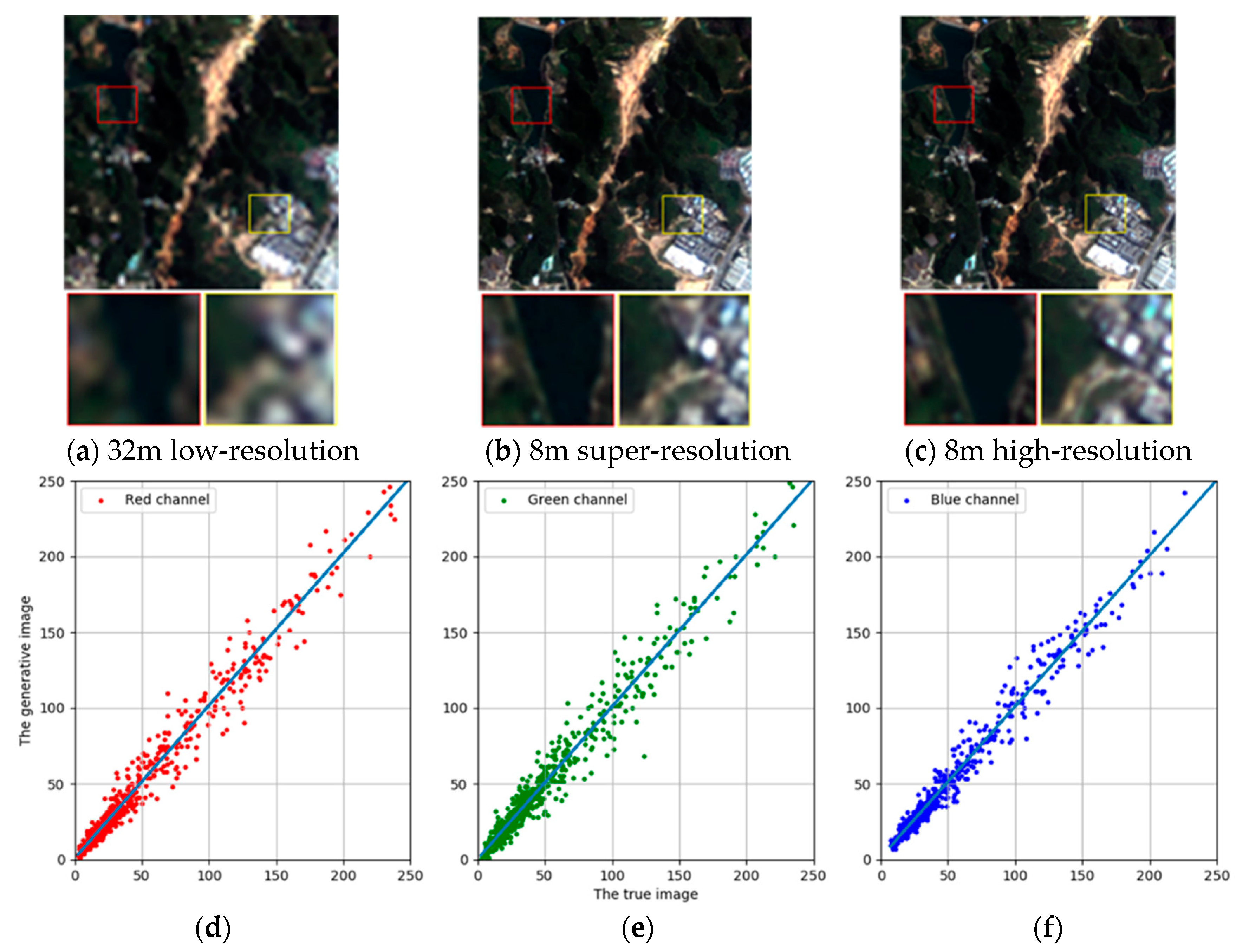
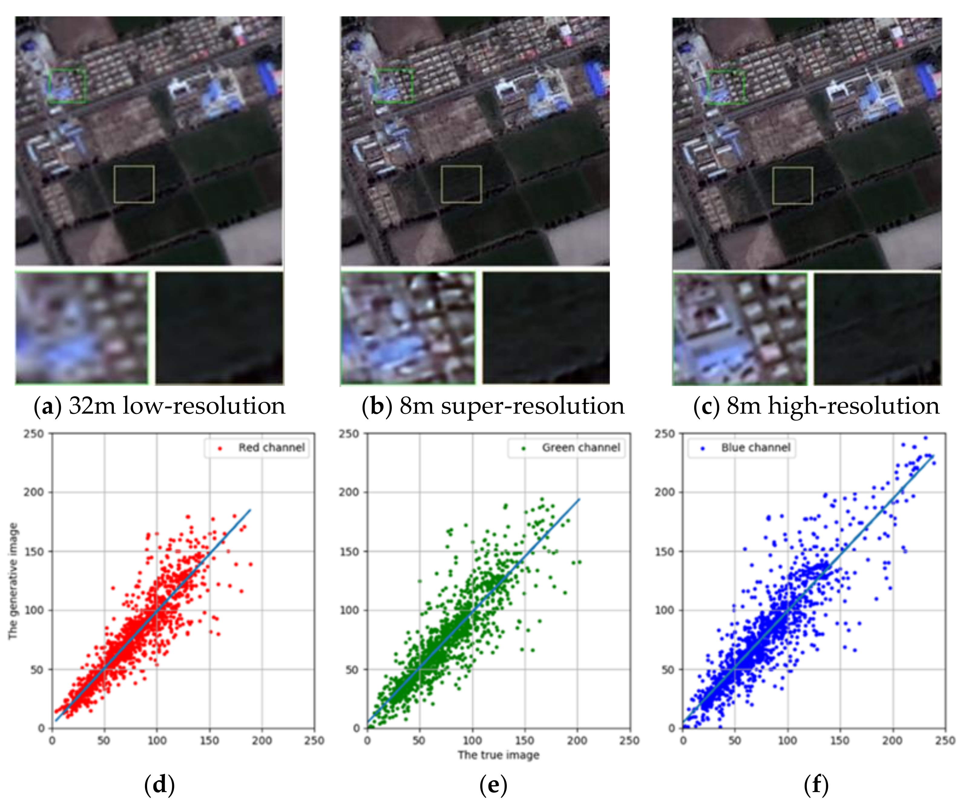
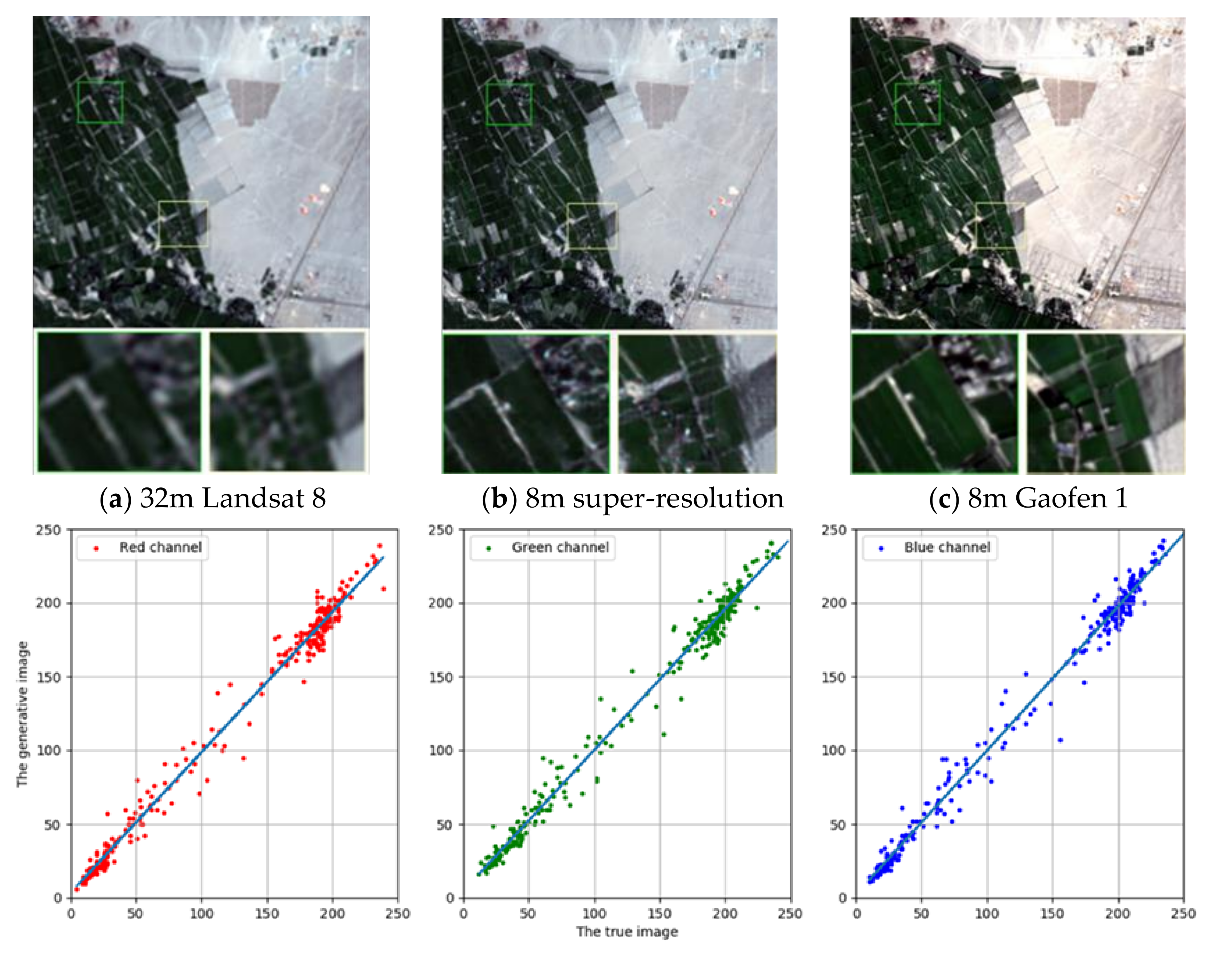
Based on the ISRGAN super-resolution training model, we tested the ISRGAN on a GF 1 dataset from Guangdong, a GF 1 dataset in Xinjiang, and a Landsat 8 dataset in Xinjiang. Some test results are shown in Figure 4, Figure 5 and Figure 6.

As can be seen from the examples, the slope of the statistical pictures of the image after super-resolution and the real image in the gray value of the three bands is close to 1, so this model maintains the spectral information of the original image.

In addition, in order to verify the generalization ability of the super-resolution model across locations and sensors, we defined the following: if the evaluation indexes on two data sets follow a normal distribution and the mean value is not significantly different, then the model is approximately considered to have the same property on two datasets. Therefore, when verifying the generalization ability of the model across locations, we conducted t-tests on the evaluation indexes of the Guangdong (GF 1) dataset and the Xinjiang (GF 1) dataset. When verifying the generalization ability of the model across sensors, we also conducted a t-test on the evaluation indexes of the Xinjiang (GF 1) dataset and the Xinjiang (Landsat) dataset by using the R software with the “car” package (https://www.rdocumentation.org/packages/car/versions/3.0-3), for which the confidence was 95%. The test results are shown in

Table 5. T-Test of the model across locations.

		Levene Test of Variance	T-Test of the Mean
		Sig	Sig(2-tailed)
SSIM	Variances are equal	0.510	1.000
	Variances are not equal		1.000
PSNR	Variances are equal	0.033	0.621
	Variances are not equal		0.625

and

Table 6. T-Test of the model across sensors.

		Levene Test of Variance	T-Test of the Mean
		Sig	Sig(2-tailed)
SSIM	Variances are equal	0.011	0.824
	Variances are not equal		0.826
PSNR	Variances are equal	0.197	0.000
	Variances are not equal		0.000

, respectively.

In Table 5 and Table 6, first, we judge whether there is a significant difference between the two groups of data, which is the Levene test of the variance equation. If the Sig parameter values are greater than 0.05, there is no significant difference in variance. After judging the variance, a t-test was performed on the mean value. Similarly, if the Sig (2-tailed) index value is greater than 0.05, there is no significant difference in the mean value of the two groups of data, which means that there is no significant difference between the two groups of data. As can be seen from Table 5, there is no significant difference in the mean values of the two groups of data in the PSNR and SSIM. Therefore, the model has generalization ability across locations. As can be seen from Table 6, there is no significant difference between the two groups of data in the SSIM, while there is a significant difference between the two groups of data in the PSNR. Since the PSNR only considers the gray value of pixels between the two groups of images, while the SSIM comprehensively considers the brightness, contrast, structure, and other information between the two groups of images, the SSIM has generalization ability across sensors.

4.2. Compare ISRGAN with NE, SCSR, and SRGAN

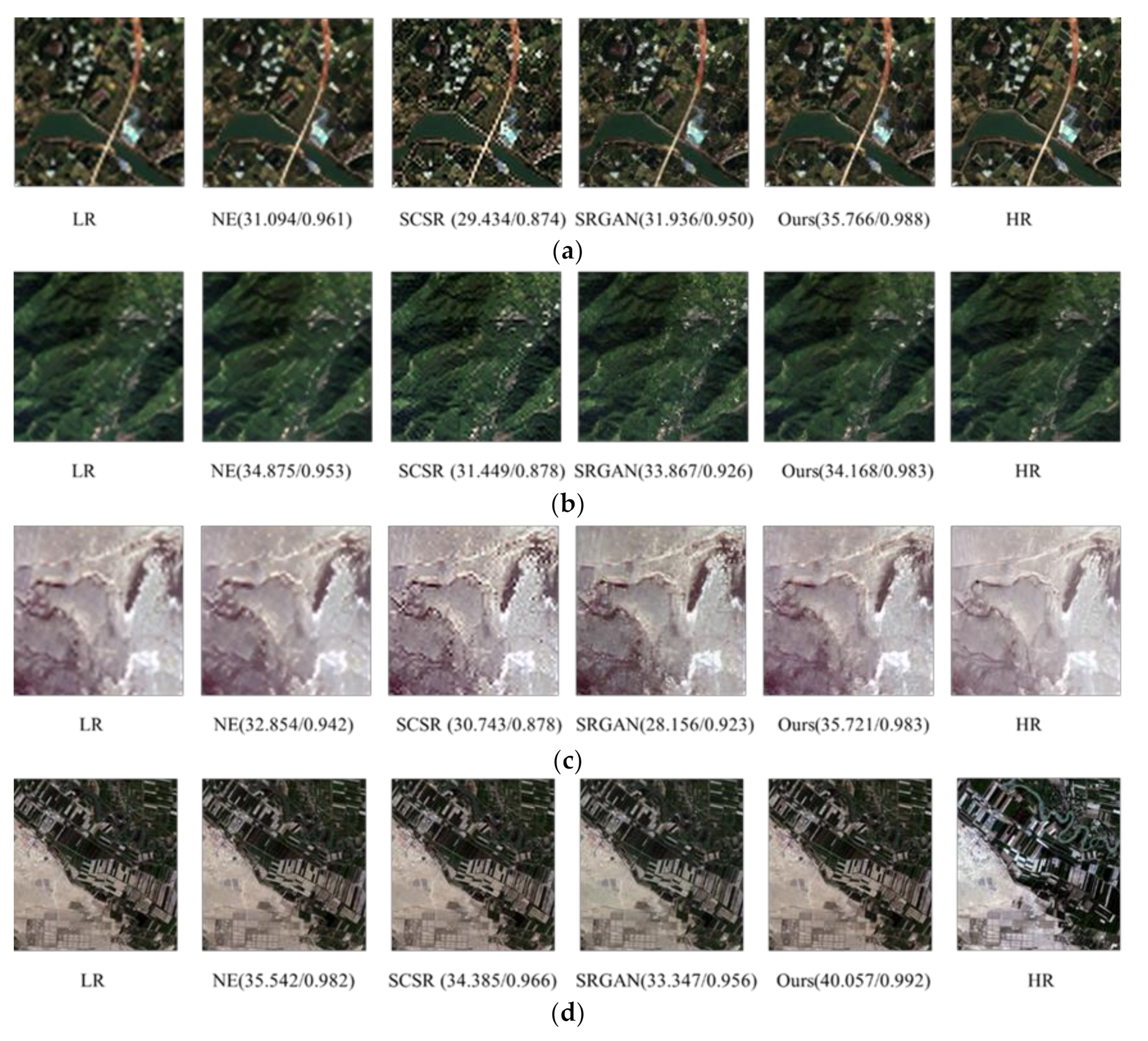
In this paper, the super-resolution methods we compared include the NE and SCSR methods, and the SRGAN. According to the super-resolution results, we calculated the evaluation indexes between them and the original images. In this paper, it was difficult to obtain the Landsat 8 satellite data and GF 1 satellite data at the same time and in the same scene, and the corresponding number of pixels was not consistent, considering the subsequent consistency of the computational criteria in validating whether the model has generalization ability across locations and sensors. Therefore, all the reference images of the quantitative calculation in this paper were the original images before super-resolution. The calculation method was to reduce the sampling of the image after super-resolution and then calculate the quantification index between the image after super-resolution and the original image. Figure 7 shows the partial comparison results of this paper based on the NE and SCSR methods, the SRGAN, and the ISRGAN in the three test sets.

We counted the evaluation indexes of the test data on the three test sets with three super-resolution algorithms and calculated their means. The results are shown in

Table 7. Image quality comparison of different super-resolution algorithms.

Data Sets	Index	NE	Super-Resolution Algorithms
			SCSR	SRGAN	Ours
Guangdong (GF 1)	PSNR	33.6349	31.1207	32.1658	36.3744
	SSIM	0.9600	0.8854	0.9375	0.9884
Xinjiang (GF 1)	PSNR	32.0343	30.1631	31.3782	35.8160
	SSIM	0.9608	0.9001	0.9524	0.9885
Xinjiang (Landsat 8)	PSNR	35.0010	33.639	32.8203	38.0922
	SSIM	0.9818	0.9654	0.9488	0.9879

:

As can be seen from Table 7, in the horizontal comparison of the three super-resolution algorithms, the ISRGAN algorithm in this paper is significantly superior to the other three methods in the PSNR and SSIM, so it has certain advantages.

4.3. The Improvement of Land Cover Classification after ISRGAN Super-Resolution

The purpose of image super-resolution is to make better use of the advantages of high spatial resolution images and improve the accuracy of target recognition [36], classification [37], and change detection [38,39]. Taking the land cover classification and ground feature extraction as examples, the changes in the land use classification and ground feature extraction in the Landsat images before and after super-resolution were compared and analyzed.

The classification area selected was in the area at the border of Guangzhou and Shenzhen, where the feature categories are rich and densely distributed. It is beneficial to fully take advantage of high spatial resolution images in the land use classification and feature extraction. As shown in Figure 8, the original Landsat 8 image of the super-resolution application sample area was obtained on February 7, 2016.

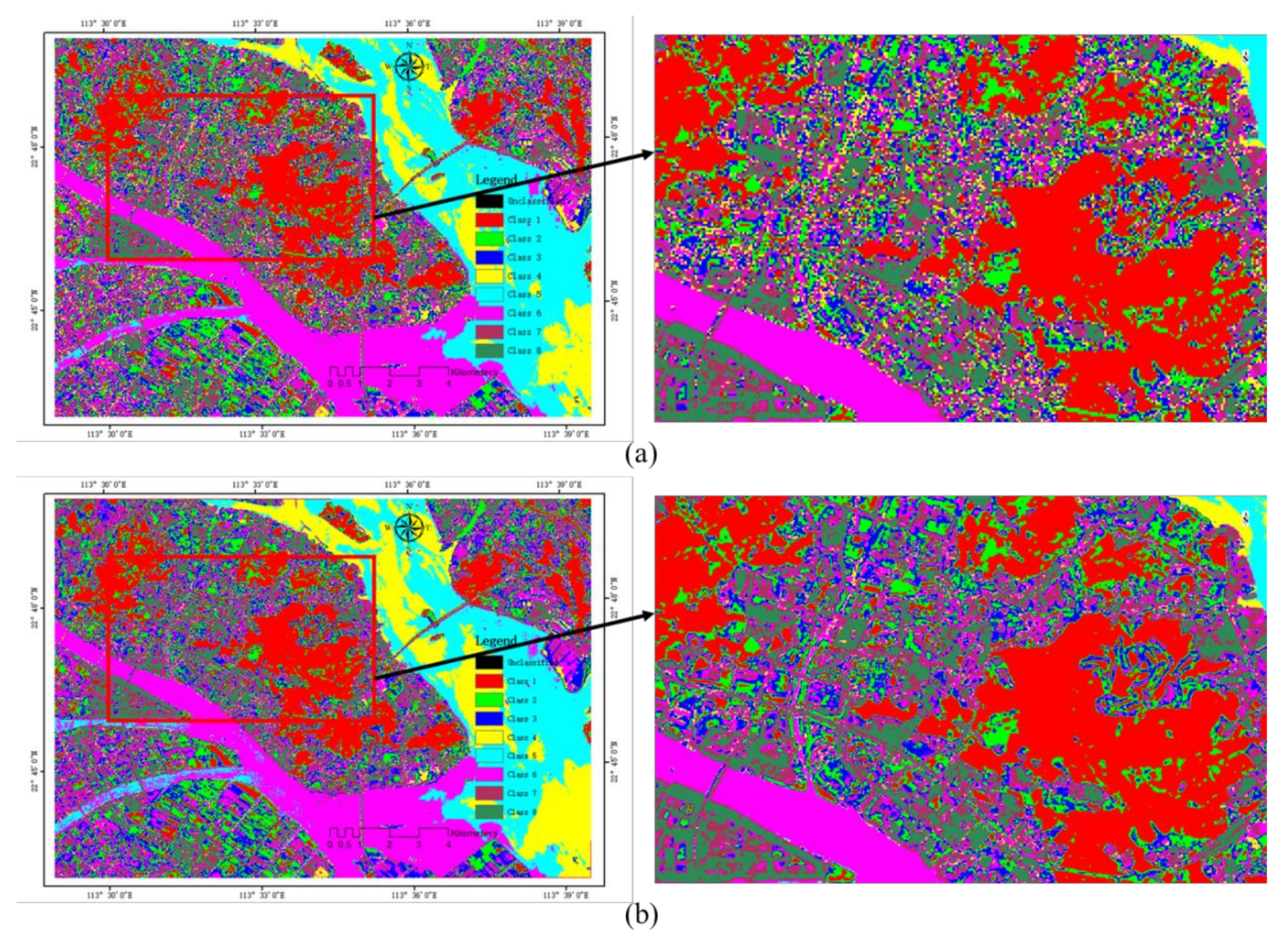
For the classification of features, in order to avoid the interference of human factors on the classification results, we used the K-means algorithm to classify the before and after images of super-resolution, and the classification results are shown in Figure 9.

By comparing the classification results before and after the super-resolution images, we can see that the extraction effect of the image after super-resolution is better than that before super-resolution in the areas where the features are densely distributed and texture details are not obvious, such as roads and impervious surfaces. From the overall extraction effect, the result of the image after the super-resolution classification is better than that of the former in boundary and separability. Therefore, the image after super-resolution is broadly applicable in the classification of remote sensing images.

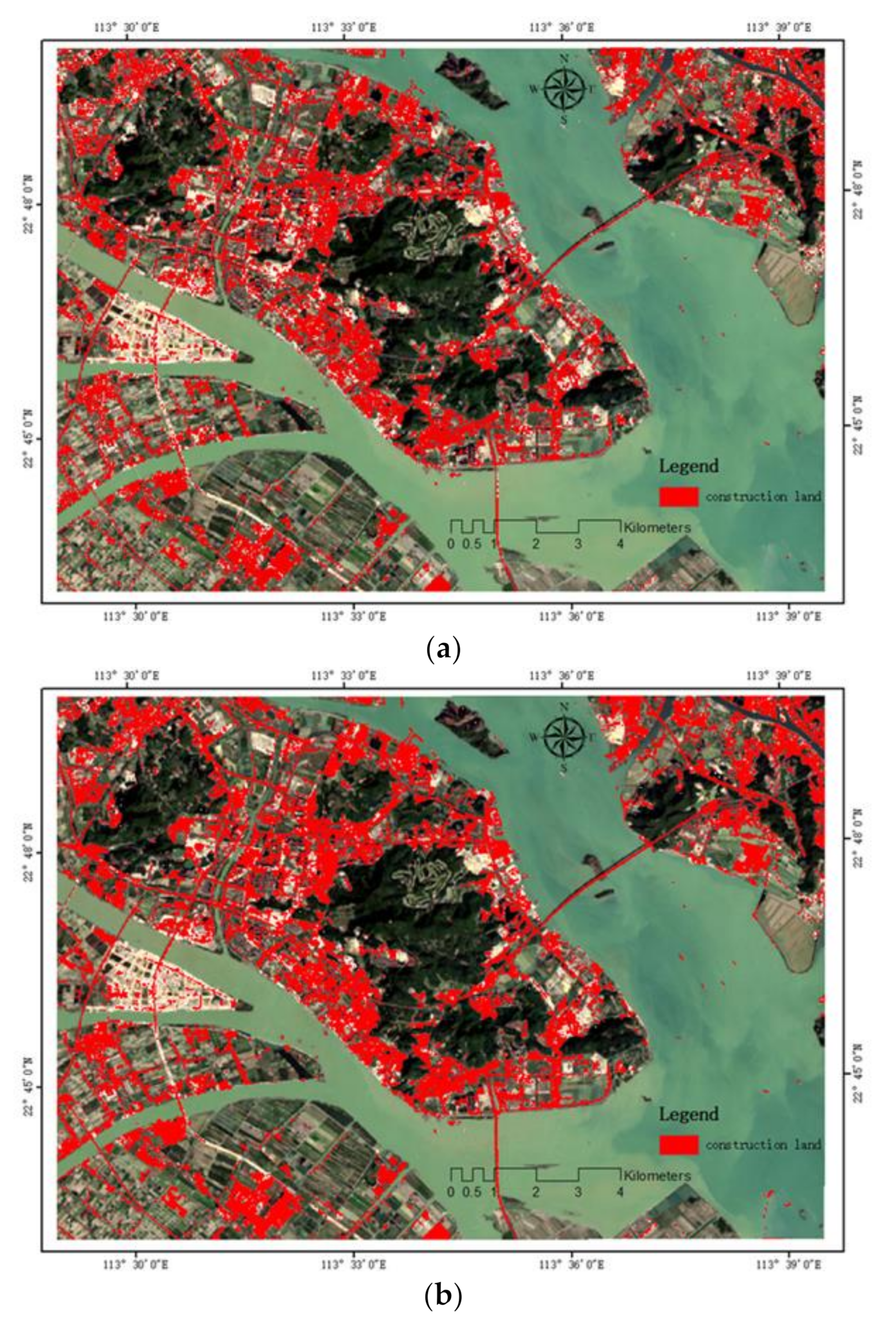
In addition, in order to better reflect the superiority of the image after super-resolution on the extraction of impervious surfaces, we used the Support Vector Machine (SVM) algorithm to extract impervious surfaces based on images before and after super-resolution. Similarly, in order to minimize the influence of human factors on the extraction results, we randomly selected the same set of training samples and test samples on Google Earth, converted them into the area of interest at the corresponding resolution, and then classified and extracted them. The extraction results of the impervious surfaces before and after super-resolution are shown in Figure 10.

In order to quantitatively verify the improvement of the extraction accuracy of impervious surfaces based on the image after super-resolution, we tested the same set of test samples selected above, which included 122 impervious surface sample points and 71 non-impervious surface sample points. The confusion matrix of the impervious surface extraction before and after super-resolution is shown in

Table 8. Confusion matrix of construction on the image before super-resolution.

Class	Impervious Surface	Others
Impervious Surface	61.48%	15.28%
Others	38.52%	84.71%

and

Table 9. Confusion matrix of construction on the image after super-resolution.

Class	Impervious Surface	Others
Impervious Surface	79.51%	2.78%
Others	20.49%	97.22%

. The overall accuracy of the impervious surface extraction before super-resolution was 70.1%, and the Kappa coefficient was 0.419. After super-resolution, the overall extraction accuracy of impervious surfaces was 86.1%, and the Kappa coefficient was 0.720. The quantitative results show that the extraction accuracy after super-resolution was nearly 15% higher than that before super-resolution.

5. Discussion

In comparison with the NE method, SCSR method, and the SRGAN, the ISRGAN shows better performance of generalization in the cross-location and -sensor tests. However, like many other super-resolution algorithms, the pseudo-textures can still be seen in the output after super-resolution, and the bell effect near the edges still needs to be improved. The edge enhancement algorithms can be further applied to recover the edge details, especially in the high spatial variation area.

Meanwhile, the scale ratio can lead to a dramatic change in the visual satisfaction of the model output. For most super-resolution algorithms, the perfect scale ratio is about 2:4. This means you can get a satisfying prediction when you down-scale an image with 30-m resolution down to 8-m rather than to 1-m. By increasing this ratio, the output of the image texture could show more random pseudo-textures and lead to a more serious bell effect. The fundamental reason for this is that the learning-based super-resolution algorithms try to recover the nonlinear point spread function (PSF) from a large number of available samples. However, when the ratio increases, the image details lost when crossing the different scales could be more and more complex and harder to capture by one universal PSF based on limited samples. The process of recovering the image details by the super-resolution algorithms is ill-posed, since the number of pixels needed to be predicted always needs to be larger than the number of known low spatial resolution pixels. Other than the large-scale ratio, the other possible way to recover the image details is by using image fusion technology, such as the spatial and temporal adaptive reflectance fusion model (STARFM) [40], enhanced STARFM (ESTARFM) [41] and the U-STFM model [42], which is basically “borrowing” the detailed image texture from the high spatial resolution reference image rather than predicting it. However, the consequences are when the discrepancy between the reference image and the input image goes large or the land cover changes rapidly, and thus the fusion-based method can fail to predict these changes.

In addition, due to the fact that GANs have two networks, which are named the generator and discriminator networks, more parameters than a convolutional neural network need to be optimized during training, so a long training time is needed. Currently, Muyang Li [43] has proposed the GAN compression method, which greatly shortens the training time. Through a large number of experiments, the computations in pix2pix [44], CycleGAN [45], and GauGAN [46] with this method were reduced from 1/9 to 1/21 without losing the fidelity of the generated image in the meantime. Therefore, the GAN compression method can be applied to the super-resolution network to effectively reduce the training time of the model.

6. Conclusions

Based on the super-resolution algorithm of the generated adversarial network in the computer vision field, this paper aimed to solve the problems of gradient disappearance and mode collapse that exist in the training of the generated adversarial network itself. Combined with the method of minimizing the Wasserstein distance proposed in the WGAN, we modified the original super-resolution network (SRGAN) and proposed the ISRGAN. Then we applied it to the super-resolution of remote sensing influence and drew the following conclusions:

(1)

The ISRGAN super-resolution network proposed in this paper is applied to the super-resolution of remote sensing images, and the results obtained are better than other super-resolution methods, such as the neighbor-embedding method, the sparse representation method, and the SRGAN;

(2)

In order to realize the one-time training and repeated use of the super-resolution model, we directly applied the model trained with the Guangdong GF 1 image data to the Xinjiang GF 1 image data and conducted a t-test on the evaluation indexes of the super-resolution results of the two datasets, which verified the generalization ability of the super-resolution model across locations;

(3)

In order to combine the advantages of the domestic GF 1 image data and the Landsat 8 data, the super-resolution model trained on the GF 1 data was directly applied to the Landsat 8 data, and a t-test was performed on the evaluation indexes of the super-resolution results, verifying the generalization ability of the super-resolution model across sensors;

(4)

Taking the land use classification and ground-object extraction as examples, we compared the classification and extraction accuracy of the images before and after super-resolution. The K-means clustering algorithm was adopted for the land use classification, and the SVM algorithm was used for the ground-object extraction. The results show that the visual effect and accuracy of the images after super-resolution are improved in the classification and ground-object extraction, indicating that the super-resolution of remote sensing images is of great application value in resource development, environmental monitoring, disaster research, and global change analysis.

References

- Lim, H.S.; MatJafri, M.Z.; Abdullah, K. High spatial resolution land cover mapping using remotely sensed image. Modern Appl. Sci. 2009, 3, 82–91. [Google Scholar] [CrossRef] [Green Version]
- Mou, L.; Zhu, X.; Vakalopoulou, M.; Karantzalos, K.; Paragios, N.; Le Saux, B.; Moser, G.; Tuia, D. Multitemporal Very High Resolution From Space: Outcome of the 2016 IEEE GRSS Data Fusion Contest. IEEE J. Sel. Top. Appl. Earth Obs. Remote Sens. 2017, 10, 3435–3447. [Google Scholar] [CrossRef] [Green Version]
- Schmitt, M.; Zhu, X.X. Data Fusion and Remote Sensing: An ever-growing relationship. IEEE Geosci. Remote Sens. Mag. 2016, 4, 6–23. [Google Scholar] [CrossRef]
- Yang, D.Q.; Li, Z.M.; Xia, Y.T.; Chen, Z.Z. Remote Sensing Image Super-resolution: Challenges and Approaches. In Proceedings of the 2015 IEEE International Conference on Digital Signal Processing (DSP), Singapore, 21–24 July 2015; pp. 196–200. [Google Scholar]
- Luo, Q.; Shao, X.; Peng, L.; Wang, Y.; Wang, L. Super-resolution imaging in remote sensing. Satell. Data Compress. Commun. Process. XI 2015, 9501, 950108. [Google Scholar]
- Zhang, X.G. A new kind of super-resolution reconstruction algorithm based on the ICM and the nearest neighbor interpolation. Adv. Sci. Through Comput. 2008, 344–346. [Google Scholar]
- Zhang, X.G. A New Kind of Super-Resolution Reconstruction Algorithm Based on the ICM and the Bilinear Interpolation. In Proceedings of the 2008 International Seminar on Future BioMedical Information Engineering, Wuhan, China, 18 December 2008; pp. 183–186. [Google Scholar]
- Zhang, X.G. A New Kind of Super-Resolution Reconstruction Algorithm Based on the ICM and the Bicubic Interpolation. In Proceedings of the 2008 International Symposium on Intelligent Information Technology Application Workshops, Shanghai, China, 21–22 December 2008; pp. 817–820. [Google Scholar]
- Hardie, R.C.; Barnard, K.J.; Armstrong, E.E. Joint MAP registration and high-resolution image estimation using a sequence of undersampled images. IEEE Trans. Image Process. 1997, 6, 1621–1633. [Google Scholar] [CrossRef] [Green Version]
- Tian, J.; Ma, K.K. Stochastic super-resolution image reconstruction. J. Vis. Commun. Image Represent. 2010, 21, 232–244. [Google Scholar] [CrossRef]
- Kim, K.I.; Kwon, Y. Single-image super-resolution using sparse regression and natural image prior. IEEE Trans. Pattern Anal. Mach. Intell. 2010, 32, 1127–1133. [Google Scholar]
- Kursun, O.; Favorov, O. Super-resolution by unsupervised learning of high level features in natural images. In Proceedings of the 6th World Multi-Conference on Systemics, Cybernetics and Informatics (SCI 2002)/8th International Conference on Information Systems Analysis and Synthesis (ISAS 2002), Orlando, FL, USA, 14–18 July 2002; pp. 178–183. [Google Scholar]
- Begin, I.; Ferrie, F.P. Blind super-resolution using a learning-based approach. In Proceedings of the 17th International Conference on Pattern Recognition, Cambridge, UK, 23–26 August 2004; Volume 2, pp. 85–89. [Google Scholar]
- Joshi, M.V.; Chaudhuri, S.; Panuganti, R. A learning-based method for image super-resolution from zoomed observations. IEEE Trans. Syst. Man Cybern. Part B Cybern. 2005, 35, 527–537. [Google Scholar] [CrossRef]
- Chan, T.M.; Zhang, J.P. An improved super-resolution with manifold learning and histogram matching. In International Conference on Biometrics; Springer: Berlin/Heidelberg, Germany, 2006; pp. 756–762. [Google Scholar]
- Rajaram, S.; Das Gupta, M.; Petrovic, N.; Huang, T.S. Learning-based nonparametric image super-resolution. EURASIP J. Appl. Signal Process. 2006, 51306. [Google Scholar] [CrossRef] [Green Version]
- Kim, C.; Choi, K.; Ra, J.B. Improvement on Learning-Based Super-Resolution by Adopting Residual Information and Patch Reliability. In Proceedings of the 2009 16th IEEE International Conference on Image Processing, Cairo, Egypt, 7–10 November 2009; pp. 1197–1200. [Google Scholar]
- Yang, M.C.; Chu, C.T.; Wang, Y.C.F. Learning Sparse Image Representation with Support Vector Regression for Single-Image Super-Resolution. In Proceedings of the 2010 IEEE International Conference on Image Processing, Hong Kong, China, 26–29 September 2010; pp. 1973–1976. [Google Scholar]
- Zhang, J.; Zhao, C.; Xiong, R.Q.; Ma, S.W.; Zhao, D.B. Image Super-Resolution Via Dual-Dictionary Learning and Sparse Representation. In Proceedings of the 2012 IEEE International Symposium on Circuits and Systems (ISCAS), Seoul, Korea, 20–23 May 2012; pp. 1688–1691. [Google Scholar]
- Dong, C.; Loy CC, G.; He, K.M.; Tang, X.O. Learning a Deep Convolutional Network for Image Super-Resolution. In European Conference on Computer Vision; Springer: Cham, Switzerland, 2014; pp. 184–199. [Google Scholar]
- Chang, H.; Yeung, D.Y.; Xiong, Y. Super-resolution through neighbor embedding. In Proceedings of the 2004 IEEE Computer Society Conference on Computer Vision and Pattern Recognition, Washington, DC, USA, 27 June–2 July 2004; Volume 1, pp. 275–282. [Google Scholar]
- Yang, J.; Wright, J.; Huang, T.S.; Ma, Y. Image super-resolution via sparse representation. IEEE Trans. Image Process. 2010, 19, 2861–2873. [Google Scholar] [CrossRef] [PubMed]
- Miskin, J.; MacKay, D.C. Ensemble Learning for Blind Image Separation and Deconvolution. In Advances in Independent Component Analysis; Springer: London, UK, 2000; pp. 123–141. [Google Scholar]
- Guo, S.; Sun, B.; Zhang, H.K.; Liu, J.; Chen, J.; Wang, J.; Jiang, X.; Yang, Y. MODIS ocean color product downscaling via spatio-temporal fusion and regression: The case of chlorophyll-a in coastal waters. Int. J. Appl. Earth Obs. Geoinf. 2018, 73, 340–361. [Google Scholar] [CrossRef]
- Dong, C.; Loy, C.C.; He, K. Image Super-Resolution Using Deep Convolutional Networks. IEEE Trans. Pattern Anal. Mach. Intell. 2016, 38, 295–307. [Google Scholar] [CrossRef] [PubMed] [Green Version]
- Lu, Y.; Qin, X.S. A coupled K-nearest neighbour and Bayesian neural network model for daily rainfall downscaling. Int. J. Climatol. 2014, 34, 3221–3236. [Google Scholar] [CrossRef]
- Takeda, H.; Farsiu, S.; Milanfar, P. Kernel regression for image processing and reconstruction. IEEE Trans. Image Process. 2007, 16, 349–366. [Google Scholar] [CrossRef] [PubMed] [Green Version]
- Zhang, H.; Huang, B. Support vector regression-based downscaling for intercalibration of multiresolution satellite images. IEEE Trans. Geosci. Remote Sens. 2013, 51, 1114–1123. [Google Scholar] [CrossRef]
- Ledig, C.; Theis, L.; Huszar, F.; Caballero, J.; Cunningham, A.; Acosta, A.; Aitken, A.; Tejani, A.; Totz, J.; Wang, Z.H.; et al. Photo-Realistic Single Image Super-Resolution Using a Generative Adversarial Network. In Proceedings of the IEEE Conference on Computer Vision and Pattern Recognition, Honolulu, HI, USA, 21–26 July 2017; pp. 105–114. [Google Scholar]
- Goodfellow, I.J.; Pouget-Abadie, J.; Mirza, M.; Xu, B.; Warde-Farley, D.; Ozair, S.; Courville, A.; Bengio, Y. Generative Adversarial Nets. In Proceedings of the NIPS’14: 27th International Conference on Neural Information Processing Systems; MIT Press: Cambridge, MA, USA, 2014; pp. 2672–2680. [Google Scholar]
- He, K.; Zhang, X.; Ren, S.; Sun, J. Deep residual learning for image recognition. In Proceedings of the 2016 IEEE Conference on Computer Vision and Pattern Recognition (CVPR), Las Vegas, NV, USA, 26 June–1 July 2016; pp. 770–778. [Google Scholar]
- Simonyan, K.; Zisserman, A. Very Deep Convolutional Networks for Large-Scale Image Recognition. arXiv 2014, arXiv:1409.1556. [Google Scholar]
- Arjovsky, M.; Chintala, S.; Bottou, L. Wasserstein GAN. arXiv 2017, arXiv:1701.07875. [Google Scholar]
- Steele, R. Peak Signal-to-Noise Ratio Formulas for Multistage Delta Modulation with Rc-Shaped Gaussian Input Signals. Bell Syst. Tech. J. 1982, 61, 347–362. [Google Scholar] [CrossRef]
- Wang, Z.; Bovik, A.C.; Sheikh, H.R.; Simoncelli, E.P. Image quality assessment: From error visibility to structural similarity. IEEE Trans. Image Process. 2004, 13, 600–612. [Google Scholar] [CrossRef] [Green Version]
- Coulter, L.L.; Stow, D.A. Monitoring habitat preserves in southern California using high spatial resolution multispectral imagery. Environ. Monit. Assess. 2009, 152, 343–356. [Google Scholar] [CrossRef] [PubMed]
- Chang, C.W.; Shi, C.H.; Liew, S.C.; Kwoh, L.K. Land Cover Classification of Very High Spatial Resolution Satelite Imagery. In Proceedings of the 2013 IEEE International Geoscience and Remote Sensing Symposium—IGARSS, Melbourne, Australia, 21–26 July 2013; pp. 2685–2687. [Google Scholar]
- Lu, D.; Hetrick, S.; Moran, E.; Li, G. Detection of urban expansion in an urban-rural landscape with multitemporal QuickBird images. J. Appl. Remote Sens. 2010, 4, 041880. [Google Scholar] [CrossRef] [PubMed] [Green Version]
- Coppin, P.; Jonckheere, I.; Nackaerts, K.; Muys, B.; Lambin, E. Digital change detection methods in ecosystem monitoring: A review. Int. J. Remote Sens. 2004, 25, 1565–1596. [Google Scholar] [CrossRef]
- Gao, F.; Masek, J.; Schwaller, M.; Hall, F. On the Blending of the Landsat and MODIS Surface Reflectance: Predicting Daily Landsat Surface Reflectance. IEEE Trans. Geosci. Remote Sens. 2006, 44, 2207–2218. [Google Scholar]
- Zhu, X.; Chen, J.; Gao, F.; Chen, X.; Masek, J.G. An enhanced spatial and temporal adaptive reflectance fusion model for complex heterogeneous regions. Remote Sens. Environ. 2010, 114, 2610–2623. [Google Scholar] [CrossRef]
- Huang, B.; Zhang, H. Spatio-temporal reflectance fusion via unmixing: Accounting for both phenological and land-cover changes. Int. J. Remote Sens. 2014, 35, 6213–6233. [Google Scholar] [CrossRef]
- Li, M.; Lin, J.; Ding, Y.; Liu, Z.; Zhu, J.Y.; Han, S. GAN Compression: Efficient Architectures for Interactive Conditional GANs. arXiv 2020, arXiv:2003.08936. [Google Scholar]
- Isola, P.; Zhu, J.Y.; Zhou, T.; Efros, A.A. Image-to-Image Translation with Conditional Adversarial Networks. In Proceedings of the 2017 IEEE Conference on Computer Vision and Pattern Recognition (CVPR), Honolulu, HI, USA, 21–26 July 2017; pp. 5967–5976. [Google Scholar]
- Zhu, J.Y.; Park, T.; Isola, P.; Efros, A.A. Unpaired Image-to-Image Translation using Cycle-Consistent Adversarial Networks Jun-Yan. In Proceedings of the IEEE International Conference on Computer Vision, Venice, Italy, 22–29 October 2017; pp. 2223–2232. [Google Scholar]
- Park, T.; Liu, M.Y.; Wang, T.C.; Zhu, J.Y. Semantic image synthesis with spatially-adaptive normalization. In Proceedings of the IEEE Conference on Computer Vision and Pattern Recognition, Long Beach, CA, USA, 16–20 June 2019; pp. 2332–2341. [Google Scholar]
Figure 1.
The workflow of the experiment.
Figure 2.
The typical structure of generative adversarial nets (GANs) adapted from [30].
Figure 3.
Study area and the image coverage of GF 1.
Figure 4.
The predicted super-resolution image for our ISRGAN model (b) on a GF 1 dataset in Guangdong, compared to the input image (a) and the ground truth (c). Figures (d), (e), and (f) are 1:1 plots of the Digital Number (DN) value in the red, green and blue bands compared to the ground truth (c), with slopes of 1.0063, 1.0032, and 0.9955, respectively.
Figure 5.
Cross-location comparison: the predicted super-resolution image for our ISRGAN model (b) on a GF 1 dataset in Xinjiang, compared to the input image (a) and the ground truth (c). Figures (d), (e), and (f) are 1:1 plots of the DN value in the red, green and blue bands compared to the ground truth (c), with slopes of 0.9658, 0.9378 and 0.9485, respectively.
Figure 6.
Cross-sensor and -location comparison: the predicted super-resolution image for our ISRGAN model (b) on a Landsat 8 dataset in Xinjiang, compared to the input image (a) and the ground truth (c). Figures (d), (e), and (f) are 1:1 plots of the DN value in the red, green and blue bands compared to the ground truth (c), with slopes of 0.9527, 0.9564 and 0.9760, respectively.
Figure 7.
Comparison of the output of our ISRGAN model (the fifth column) to other models (NE, SCSR, SRGAN). Figures (a) and (b) are the results of the GF 1 dataset in Guangdong, (c) is the result of the cross-location testing in the GF 1 dataset in Xinjiang, and (d) is the result of Landsat 8 in Xinjiang. The ground truth is shown as HR. The low-resolution inputs are marked as LR.
Figure 8.
Landsat 8 image of the demonstration area.
Figure 9.
Comparison of the classification results between the images before and after super-resolution. Figure (a) is the classification result on the image before super-resolution and Figure (b) is the classification result on the image after super-resolution.
Figure 10.
Comparison of the extraction results of impervious surfaces between the images before and after super-resolution (Figure (a) is the extraction result on the image before super-resolution and Figure (b) is the extraction result on the image after super-resolution).