Article

Phenological Characterization of Desert Sky Island Vegetation Communities with Remotely Sensed and Climate Time Series Data

by
Willem J.D. Van Leeuwen
1,2,*,
Jennifer E. Davison
1,
Grant M. Casady
1 and
Stuart E. Marsh
1,2
1
School of Natural Resources and the Environment, University of Arizona, Tucson AZ, 85721, USA
2
School of Geography and Development, University of Arizona, Tucson AZ, 85721, USA
*
Author to whom correspondence should be addressed.
Remote Sens. 2010, 2(2), 388-415; https://doi.org/10.3390/rs2020388
Submission received: 1 December 2009 / Revised: 15 January 2010 / Accepted: 21 January 2010 / Published: 27 January 2010
(This article belongs to the Special Issue Ecological Status and Change by Remote Sensing)

Abstract

:
Climate change and variability are expected to impact the synchronicity and interactions between the Sonoran Desert and the forested sky islands which represent steep biological and environmental gradients. The main objectives were to examine how well satellite greenness time series data and derived phenological metrics (e.g., season start, peak greenness) can characterize specific vegetation communities across an elevation gradient, and to examine the interactions between climate and phenological metrics for each vegetation community. We found that representative vegetation types (11), varying between desert scrub, mesquite, grassland, mixed oak, juniper and pine, often had unique seasonal and interannual phenological trajectories and spatial patterns. Satellite derived land surface phenometrics (11) for each of the vegetation communities along the cline showed numerous distinct significant relationships in response to temperature (4) and precipitation (7) metrics. Satellite-derived sky island vegetation phenology can help assess and monitor vegetation dynamics and provide unique indicators of climate variability and patterns of change.

1. Introduction

Climate patterns from intra-seasonal to decadal and century scales directly influence the timing, magnitude (productivity), and spatial patterns of vegetation growth cycles, or phenology [1,2]. Vegetation phenology can be detected by satellites and other remote sensing systems due to the unique seasonal and spectral reflectance and transmittance characteristics of canopy, plants and leaves [1,3]. Compared to other land surface components (e.g., soils), red and NIR reflectance values for green vegetation are low and high respectively. The Normalized Difference Vegetation Index (NDVI = (ρNIR – ρred)/(ρNIR + ρred)) [4] is one of the most commonly used spectral vegetation indices for agricultural and natural resource monitoring applications and has been related to many biophysical properties, such as fractional green cover, chlorophyll density and leaf-area index (LAI), the fraction of absorbed photosynthetically active radiation (fAPAR), biomass and net primary production [5,6,7,8]. Remotely sensed vegetation phenological data have been used in global climate change studies, showing trends and responses such as earlier start of the growing season, later end of season, and higher seasonal productivity [9,10]. In addition, remotely sensed vegetation phenology information is used to determine land cover classes [11,12] and vegetation dynamics in response to climate [13] and disturbances and stressors like fire [14] and drought [15]. Metrics created from spectral vegetation indices, such as start of season, peak index or greenness value, and seasonal integrated greenness are used in many models and studies to describe phenology and to represent vegetation interactions with climate-based [5,10,16] and anthropogenic [17,18] factors.
Most remote sensing phenology studies use satellite-based vegetation index (VI) time series as a source to derive phenological metrics (phenometrics) to identify critical measures (e.g., timing of start, peak, length of the growing season, amounts of greenness) in the annual seasonal vegetation index signatures that match phenological phases of vegetation development. Many algorithms have been designed to retrieve phenometrics [19]. Jönsson and Eklundh [20,21] designed a phenometrics retrieval approach that is based on both threshold and curve derivative methods. This approach reduces residual atmospheric noise in the time series data, and provides a user-friendly output in either a point-based or image format.

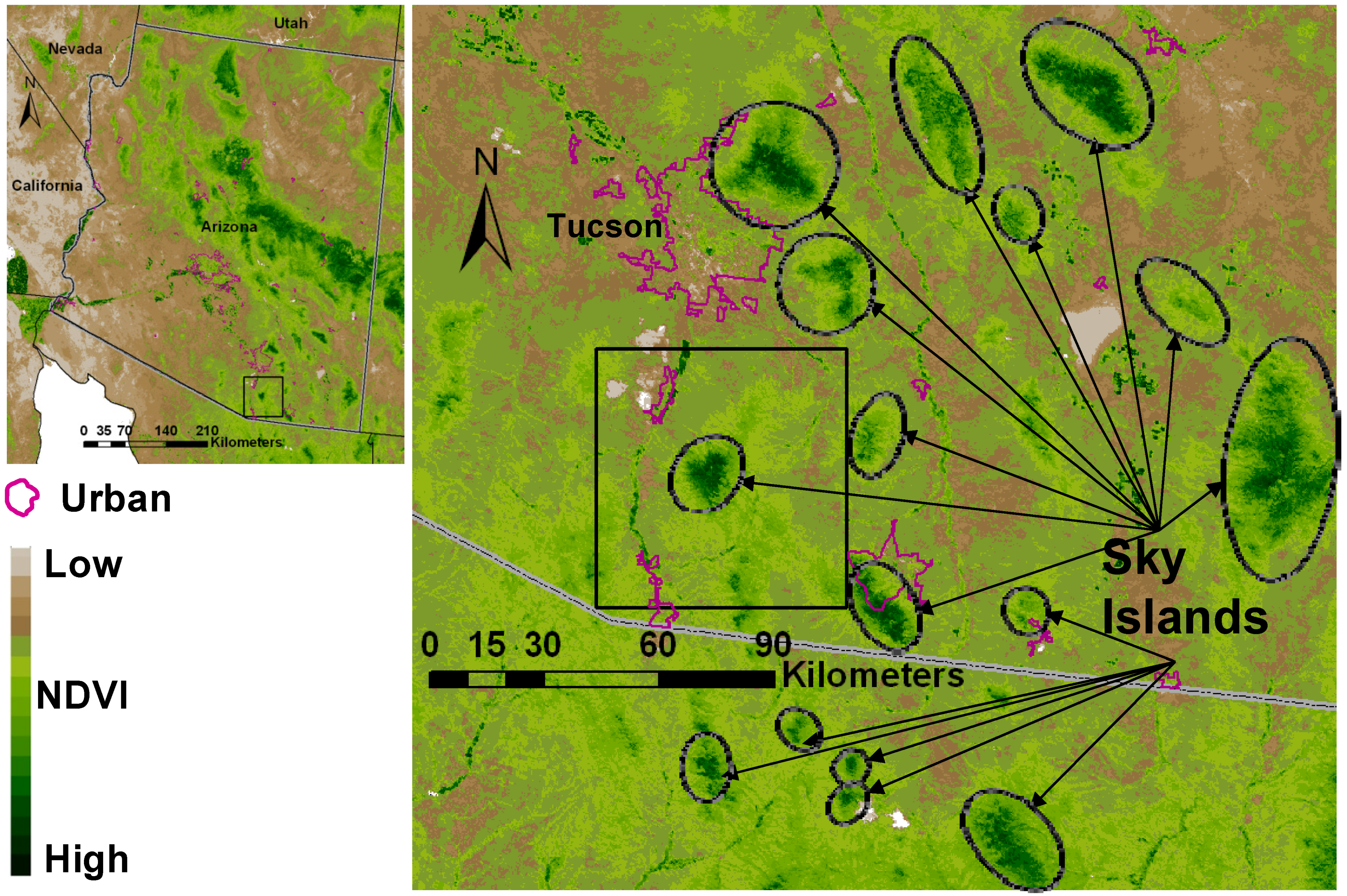
1.1. Nature of the Study Area

Sky islands are biogeographically isolated mountains, which are connected by lowland valleys and terrain that act as both barriers and bridges to dispersion and colonization by new species from one mountain or valley to another mountain or valley. Many sky islands throughout the world have resulted from isolation caused by erosive and tectonic forces over time and the interplay with varied bedrock formations [22]. Sky islands contain a large number of diverse landcover types [23] and contain a large part of the world’s biodiversity [24]. Drought stress and wildfire disturbance [25,26] threaten the rare and endemic species found there as well as the ecosystem functions of sky islands [27,28]. Sky islands also fulfill an important role as safe havens and food resources along bird migratory routes [29,30]. Sky islands have been shown to be regionally important as ecological regulators of water and CO2 budgets [31].
This research focused on one of the sky islands, which is part of the Madrean Archipelago, a mid-latitude inland sky island complex between the Rocky Mountains and the Sierra Madre Occidental, in the midst of the Chihuahuan and Sonoran Deserts (Figure 1). Like all sky islands, those of the Madrean Archipelago are characterized by steep ecological gradients [32,33,34].
Southeastern Arizona’s sky islands have a relatively small spatial footprint compared to the surrounding desert, with steep gradients and highly variable distribution of vegetation communities. In contrast, remotely sensed phenology data often have coarse spatial resolutions with pixels of 1 km to 1 degree in size [35]. However, the 250 m resolution NDVI time series data from the Moderate Resolution Imaging Spectroradiometer (MODIS) [36] have been used successfully for monitoring natural resources [37] and modeling vegetation response after wildfires using land surface phenological metrics [14,38,39]. Coarse global change and land classification models often exclude entire arid biomes due to the weak phenological signatures and low productivity of these areas [40]. Coarsely resolved phenological signatures may overlook small-scale patterns that indicate important ecosystem processes [41]. Thus, in research of remotely sensed vegetation phenology there is a need to further explore climate-phenology interactions to improve our understanding of the impact of climate[42] on arid lands and finer scale landscape features like sky islands.

1.2. Study Objectives

The objectives of this study were to (1) characterize and examine the variation in sky island vegetation growth and phenology patterns using satellite time series of NDVI data, (2) derive and examine vegetation type-specific phenological metrics, and (3) examine the relationship between phenometrics and climate variables along an elevation cline. We hypothesized that the timing and the magnitude of the growth cycles of vegetation communities vary according to precipitation and temperature patterns, considering that these vegetation types are mostly limited by water and insolation regimes [43]. Vegetation communities might have unique responses to these drivers that might be visible via phenometrics. Specifically, we extracted and analyzed phenological and climatic metrics for the Santa Rita Mountains, a sky island in southeastern Arizona, and (1) examined vegetation phenological characteristics for different vegetation types across a steep elevation gradient; (2) visualized spatial and temporal patterns of phenometrics; (3) examined the relationships between climate metrics (e.g., annual precipitation) and phenometrics; and (4) explored which of these phenoclimatic relationships were distinctive for specific vegetation communities.

2. Data and Methods

2.1. Study Area

The study site extent was a 4,400 km2 area south of Tucson, Arizona, which encompasses the sky island of the Santa Rita Mountains (Figure 1). The high NDVI values show the sky islands to be “refuges” in the desert “seas” (Figure 1), with a diversity of land cover types (Figure 2 [44]). The study area includes vegetation communities ranging from lowland palo verde—mixed cactus desert and mesquite grasslands to oak woodland and coniferous forest along an elevation gradient of about 2,000 m (Figure 2c). We assessed the vegetation dynamics in this area over the time span of mid-2000 through mid-2007, which allowed us to examine the growing seasons of 2001–2006.

2.2. Research Design: Sampling Land Cover, NDVI and Climate Time Series Data

Both image-based and point-based NDVI time series were examined with respect to their growth and phenology patterns. However, only areas with relatively homogeneous landcover types were selected to examine the variation in phenology and their response to climate variables. To sample the study area, several criteria were taken into account to ascertain representation of the major landcover types and avoid mixed or heterogeneous landcover patterns. The NDVI time series data were used to derive land surface phenometrics—the response variables in our modeling approach. Precipitation and temperature time series were the explanatory variables and were available at 4 km resolution. The land cover data were available at 30 m resolution and were used to stratify and select our samples that represented homogeneous areas within the same land cover type. Since the spatial resolution of the different data sets ranged from 30 m to 4,000 m, analysis was performed at the intermediate resolution of 250 m.
Figure 1. NDVI image of Arizona with a focus on the Santa Rita Mountains (pointed to in black box) and surrounding sky islands (circled), which are part of the Madrean Archipelago. The study site is centered on the Santa Rita Mountains, in southeastern Arizona, USA. The higher NDVI (Date: June 2007) values make the sky islands contrast with the Sonoran Desert lowlands. Urban areas are found within the magenta polygons.
Remotesensing 02 00388 g001

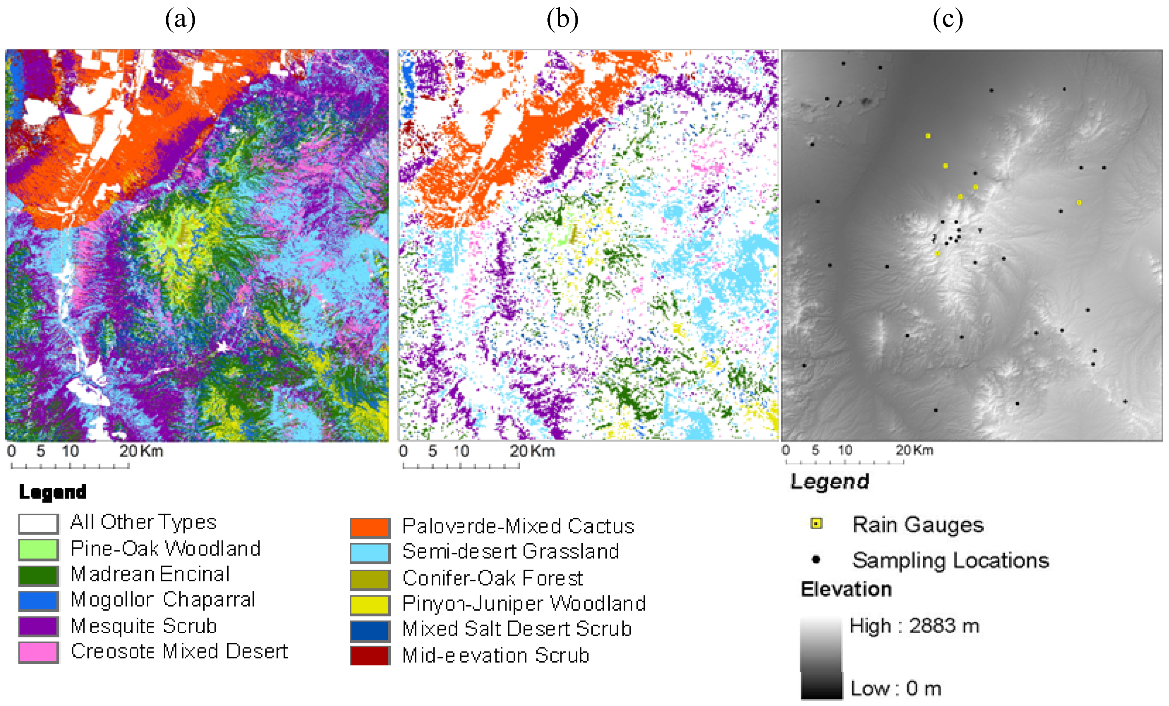
2.3. SWReGAP Landcover and DEM

To select sampling sites from which to extract time series data, we first derived vegetation community classes from the Southwestern Regional Gap Analysis Project (SWReGAP) dataset [44] (Figure 2a). The SWReGAP data were re-sampled to 250 m to match the MODIS NDVI product. The re-sampled SWReGAP product represented the majority vegetation community per MODIS pixel. We then filtered the data by analyzing the amount of contiguous 30 m SWReGAP pixels within a 250 m MODIS pixel, with at least 80% homogeneity in vegetation communities (by comparison with the original dataset). The resulting dataset included vegetation communities having at least three sites where four or more 80% homogeneous pixels were available for analysis (Figure 2b). Areas that were either non-natural or urban, and areas with high heterogeneity were not used in the analyses. The final dataset included eleven vegetation types, the full extent of which represented over 98% of the areal extent of the study site and corresponding vegetation clines, which are characteristic of many of the Sky Islands of the Madrean Archipelago. We sampled 41 sites (four pixels-25 ha-per site) throughout the study area: three to five sites per vegetation type, including six weather stations in six different vegetation types (Figure 2c).
Figure 2. (a) The vegetation communities based on the SWReGAP vegetation cover map are dominated by the 11 (b) communities used in our analysis (see also Table 1). The vegetation community data set was re-sampled to 250 m and filtered for homogeneous sites. White areas/pixels denote either developed urban and agricultural areas, or areas without enough contiguous homogeneous pixels for the analyses. (c) The locations of homogeneous sample points and weather station are distributed over the elevation gradient.
Remotesensing 02 00388 g002

2.4. MODIS NDVI Time Series

NDVI data at 250 m resolution and16-day composite intervals, acquired by MODIS on the Terra platform (MOD13Q1), were used for the NDVI time series and phenological analysis. Both the MODIS NDVI data and associated quality assurance (QA) data [36,45] were used in this research. This resulted in 23 composite NDVI and QA images (periods) per year, providing a total time series of about 161 NDVI/QA images. The MODIS NDVI images were reprojected into a Lambert Azimuth equal area projection suitable for analysis. For each of the selected homogeneous sites we extracted MODIS NDVI time series data from the 12th period of 2000 through the 11th period of 2007. Seasonal phenological metrics were then extracted for 2001 through 2006. The mean of NDVI time series data were extracted for all areas of interest excluding pixels that were affected by clouds or snow as indicated by the QA data. These data provided the basis for examining the trends, seasonality and anomalies in NDVI and the associated phenology metrics, and their relationships to climate variables, for the different land cover types.

2.5. Precipitation and Temperature

Climate data (Table 1) were extracted from Oregon State University’s Parameter Regression on Independent Slopes Model (PRISM) dataset, at 4 km spatial resolution and monthly temporal resolution [46].
Table 1. Summary of average elevation, temperature and precipitation values for each of the natural vegetation types along the Desert-Mountain gradient as described by the SWReGAP land cover project.
Ecoregion and natural landcover typeElevation (m)Tmin (°C)Tmax (°C)Annual Precip. (mm)Precip. (mm) [djfm]Precip. (mm) [amj]Precip. (mm) [jas]Precip. (mm) [on]
Sonoran Paloverde-Mixed Cacti Desert Scrub9661.237.7318.173.226.9206.824.6
Apacherian-Chihuahuan Mesquite Upland Scrub1,144−0.136.1359.182.128.3236.427.1
Sonoran Mid-Elevation Desert Scrub1,1511.836.3361.680.726.9241.728.6
Chihuahuan Creosotebush, Mixed Desert and Thorn Scrub1,333−0.435.0394.691.430.5258.329.9
Apacherian-Chihuahuan Piedmont Semi-Desert Grassland and Steppe1,358−1.334.8393.790.530.4259.928.2
Chihuahuan Mixed Salt Desert Scrub1,377−1.134.5413.794.233.0271.828.9
Madrean Encinal1,488−1.032.7490.3117.136.1318.440.5
Madrean Pinyon-Juniper Woodland1,689−2.433.0454.2105.235.9297.234.8
Mogollon Chaparral1,749−3.333.1369.682.833.3242.524.2
Madrean Pine-Oak Forest and Woodland2,204−1.531.8645.2170.442.5402.669.4
Madrean Upper Montane Conifer-Oak Forest and Woodland2,627−1.631.6702.6185.745.2437.679.8
Average monthly high and low temperature and cumulative monthly precipitation data were extracted for 2000–2006, the same time period as for the extraction of seasonal phenological metrics. To characterize the Southwestern climate patterns, both annual precipitation (January–December) and seasonal precipitation values were derived (Table 1): winter (December–March [djfm]; 4 months), a six months winter and summer (October–March and April–September), pre-monsoon (April–June; [amj]), monsoon (July–September; [jas]), and post-monsoon (October–November; [on]) [47]. We also calculated average and extreme maximum monthly temperatures, and average and extreme minimum monthly temperatures, per year and per site (Table 1).

2.6. Derivation of Phenological Metrics

Since time series of NDVI data are a proxy for recurring vegetation activity at the land surface, MODIS NDVI based phenological metrics were calculated seasonally to characterize the phenology of different vegetation types along the sky island cline. Phenometrics of the selected sites were derived by applying a local second order polynomial fitting function also known as an adaptive Savitsky-Golay filter as described by Jönsson and Eklundh [21]. We used the Savitsky-Golay smoothing filter because it was most consistent at maintaining unique vegetation time series fits while accounting for atmospheric effects like clouds. The phenometrics for each of the growing seasons, which are included in the analysis, are depicted in Figure 3.
Figure 3. NDVI observations (blue line), fitted curve (brown dashed line) and derived phenometrics: an example of the encinal oak vegetation community, Santa Rita Mountains, AZ. Startt and Endt of season are determined based on 20% of the Amplitude, set through an adjustable parameter in the TIMESAT software. Endt values generally fall at the beginning of the following calendar year.
Remotesensing 02 00388 g003
The beginning of vegetation green-up or start of the growing season, marked by Startt is defined as the point in time for which the NDVI value (StartNDVI) has increased by 20% of the distance between the left minimum NDVI value and the PeakNDVI value (Figure 3). When vegetation senesces and less vegetation cover is observed on the land surface at the end of the growing season, Endt and EndNDVI can be estimated similarly. The 20% threshold accounts for noise in the NDVI data and prevents the identification of false starts or ends of the growing seasons. The peak of a growing season is estimated by the timing of Peakt for which the NDVI value of reaches the maximum NDVI value (PeakNDVI). The amplitude of the season is obtained as the difference between the PeakNDVI value and the average of the StartNDVI has EndNDVI values. The length of season is computed as the difference between the start and end of the growing season, (Endt–Startt). Two separate integrals over the growing season are computed to estimate the production of the seasonally dominant vegetation type. The first integral (Small Integral—SI), given by the area of the region between the fitted function and the average of StartNDVI and EndNDVI values, called the BaseNDVI, represents the seasonally active vegetation, which may be large for herbaceous vegetation cover and small for evergreen vegetation cover. The second integral (Large Integral—LI), given by the area between the fitted function and the zero NDVI value bounded by the Startt and Endt, represents the total vegetation stand and is a proxy for vegetation production. The left derivative or rate of increase in NDVI during the beginning of the growing season is related to the rate of green-up and plant growth and can be estimated by calculating the ratio between the amplitude and the time difference between the start and midpoint of the growing season. The right derivative is related to the rate of senescence, but is also governed by snow cover, which can obscure green vegetation from being observed by the satellite sensor. Different vegetation cover types are likely to have different rates of green-up and senescence [48].

2.7. Data Analysis

The PRISM precipitation and temperature data were compared to data sets from six ground-based weather stations within the study sites to examine the consistency of the modeled climate data. These data were used in subsequent analyses of the relationships between phenometrics and climate variables for dominant vegetation types along the elevation cline. These stations provided monthly precipitation data from 1989 through 2006 for a total of 425 measurements. Three of the weather stations also provided measurements from 2000 through 2006, for minimum temperature (216 measurements) and maximum temperature (219 measurements). Weather station measurements were well correlated (α = 0.05) in all three datasets (R2 = 0.696, 0.928, and 0.904 for precipitation, maximum temperature, and minimum temperature, respectively).
A qualitative evaluation of the phenological characteristics for the sky island vegetation types was conducted by examining the seasonal NDVI trajectories. The spatial and temporal variation in NDVI among and within vegetation types were examined by comparing spatial patterns between wet and dry year exemplars. The difference between the wet and dry year NDVI images were used to evaluate the inter-annual spatial variability of sky island vegetation growth patterns. The inter-annual variation between the yearly phenometrics (e.g., StartNDVI Startt and LI) was quantified by the coefficient of variation (COV = standard deviation/mean). Images of COVphenometrics were computed based on each phenometric for each year between 2001 and 2006. Zero- or non-values were excluded from COV calculations. The relationships between the annually derived phenometrics and seasonal and annual climate metrics were explored using the following statistical techniques. To assess the variability of phenometrics with respect to climate and vegetation types we used correlation, MANOVA and stepwise regression analysis techniques. We used a Bonferroni adjustment to account for multiple statistical comparisons. Data were left out in instances where seasons were not detected by TIMESAT or where climate data were not available. JMP statistical software was the main tool used in our analysis (SAS Institute, 2006).

3. Results and Discussion

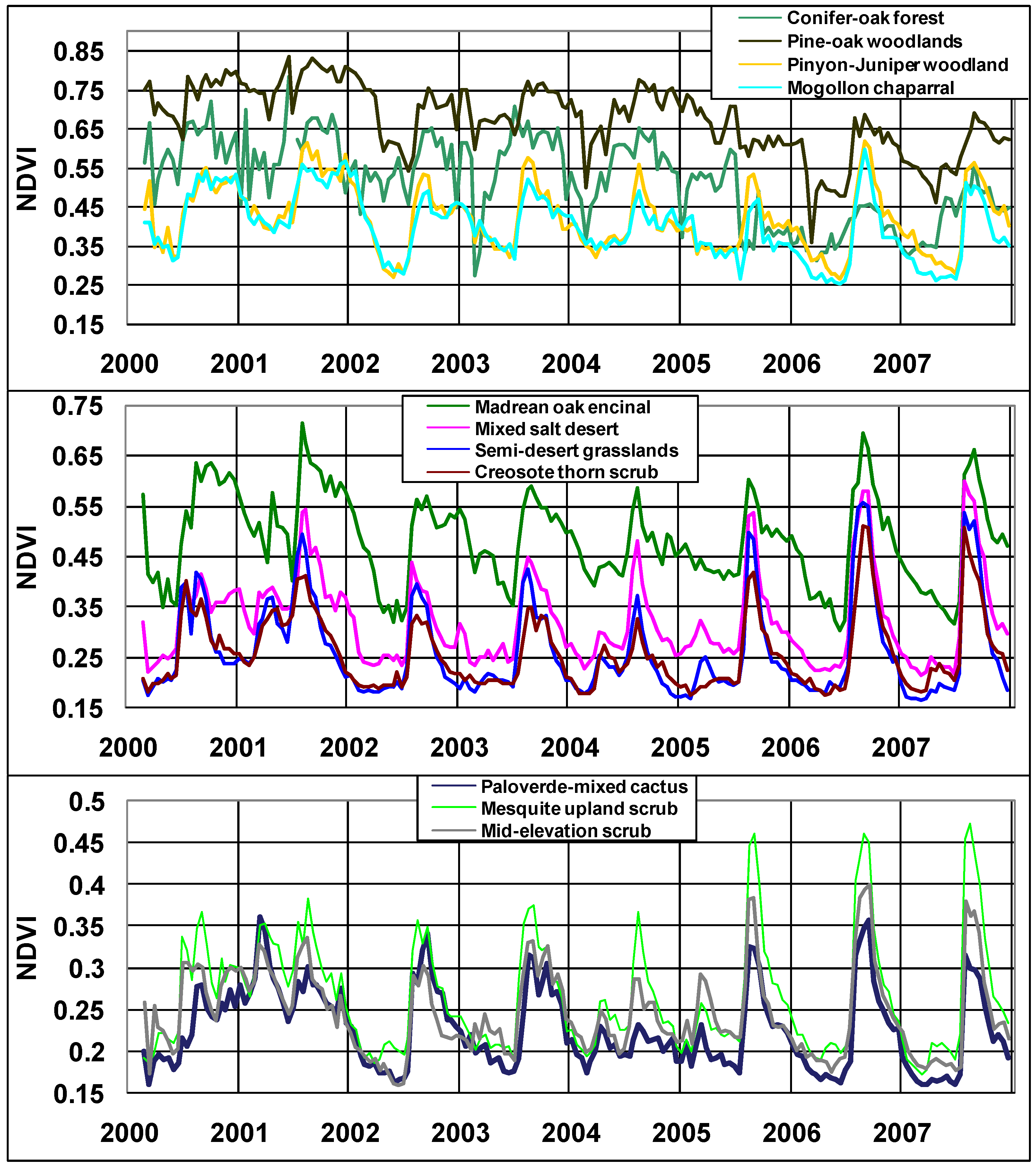
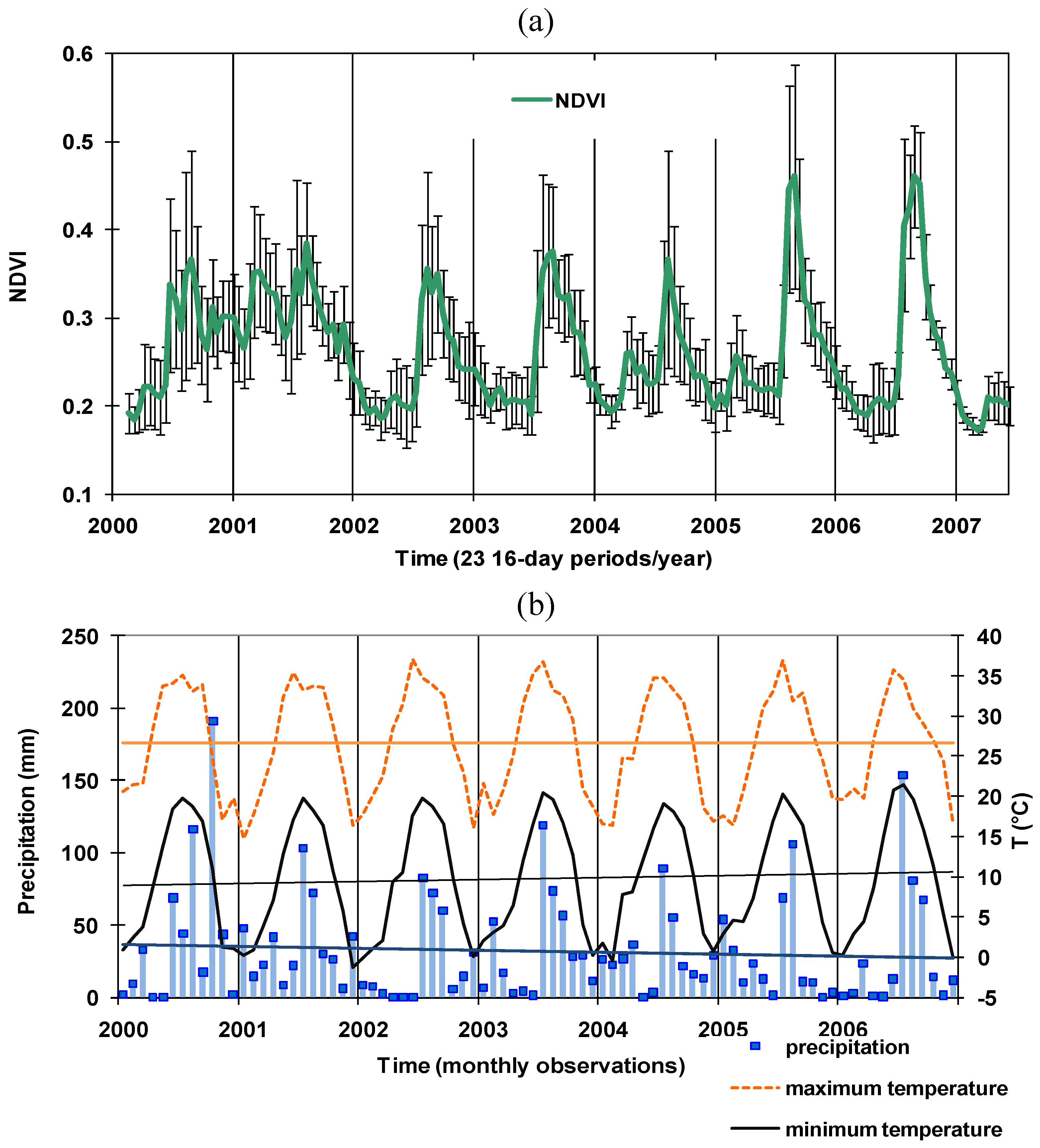
3.1. NDVI and Climate Time Series Patterns among Vegetation Types

NDVI images after the spring rainfall (May) and monsoon rainfall (September) seasons show the inter-annual, seasonal and spatial vegetation dynamics for a relatively “wet” (2001) and “dry” (2002) year (Figure 4).
Figure 4. Pre-monsoon (May; 4a–4c) and post-monsoon (September; 4d–4f) NDVI images for a wet year (2001) and a dry year (2002, especially in the spring). The difference from a multiyear NDVI average for May and September highlight below-average NDVI values (blue) for most of the study area in May, 2002. Some of the lower elevation areas show increased greenness patterns during the 2002 monsoon season (September 2002; orange patterns). Curvilinear spatial patterns represent riparian areas.
Remotesensing 02 00388 g004
Year 2001 showed a somewhat higher NDVI compared to 2002 for both May and September. However, the spatial patterns observed in the difference from yearly average (2000–2006) NDVI values for May and September of 2002 showed that overall greenness for May 2002 was much lower than average, particularly for the higher elevation areas. Generally, for September 2002 the difference from average NDVI values increased for lower elevation lands and decreased for mid-elevation lands. The riparian corridor formed by the Santa Cruz River showed a variable response to the 2002 spring drought, which might relate to a smaller effect of rainfall events.
Averaged time series data for each of the sky island vegetation types showed that the phenological signatures were generally not coinciding with each other in terms of the shape and magnitude of the NDVI response (Figure 5).
Figure 5. Average NDVI trajectories for each vegetation type, 2000–2007, Santa Rita Mountains, AZ, USA. Trends in magnitude, timing, and shape of NDVI are different for each vegetation type and each year. A high elevation forest fire in 2005 is the reason for the marked decreases in NDVI values for Conifer-oak forest and the somewhat lower NDVI values for the Pine-oak woodlands.
Remotesensing 02 00388 g005
Differences in the magnitudes of the high and low NDVI values as well as in the timing and shape of seasons can be seen among (Figure 5) and within (Figure 6) vegetation communities. Time series data also showed a high degree of variability across seasons (Figure 5). The seasonal NDVI patterns were similar for some communities and increasingly different for vegetation types that are further apart in terms of elevation range. The NDVI values generally increased with elevation. There was also strong seasonal and inter-annual NDVI variability within vegetation types.
Figure 6. (a) Mean and standard deviation of NDVI and (b) precipitation, maximum and minimum temperatures for the mesquite upland scrub vegetation type across seasons 2000–2007, Santa Rita Mountains, AZ. Effects of climate on the NDVI trajectories can be seen in a relatively wet year (2001; high NDVI) and the dry spring season (2002; low NDVI).
Remotesensing 02 00388 g006
The cross-site and inter-annual heterogeneity of the NDVI time series data highlights both the steep gradient of the Santa Rita Mountains and the variation to be expected in any vegetation community [41]. When NDVI time series were averaged for each vegetation type and compared to one another, differences in phenology could be seen that often suggested different biological or ecological processes associated with each of the vegetation types (Figure 5). For example, the phenological pattern for the pine-oak woodland showed overall higher base and peak NDVI values, less obvious seasonality and longer seasons; this could be expected in an evergreen vegetation community where seasons are often only punctuated by snow cover [1,45]. The bimodal growing season is not visible at higher elevations as the woody vegetation is rooted much deeper and responds more to temperature related cues.
Figure 6a shows an example of the variability in NDVI for sampling sites that were all classified as a mesquite community. The spring and monsoon rainfall periods resulted sometimes in a bimodal growing season, generally corresponding to weak increases in NDVI values in the spring and strong increases in NDVI values during the monsoon season. Increasing minimum night time temperatures and decreasing precipitation trends (Figure 6b) were observed to be statistically insignificant (p > 0.01) but have been predicted in the literature [27]. These climate trends, warmer summer temperatures in particular, have resulted in species flowering range changes in the Santa Catalina Mountain range, a sky island just north of the Santa Rita Mountains [50].

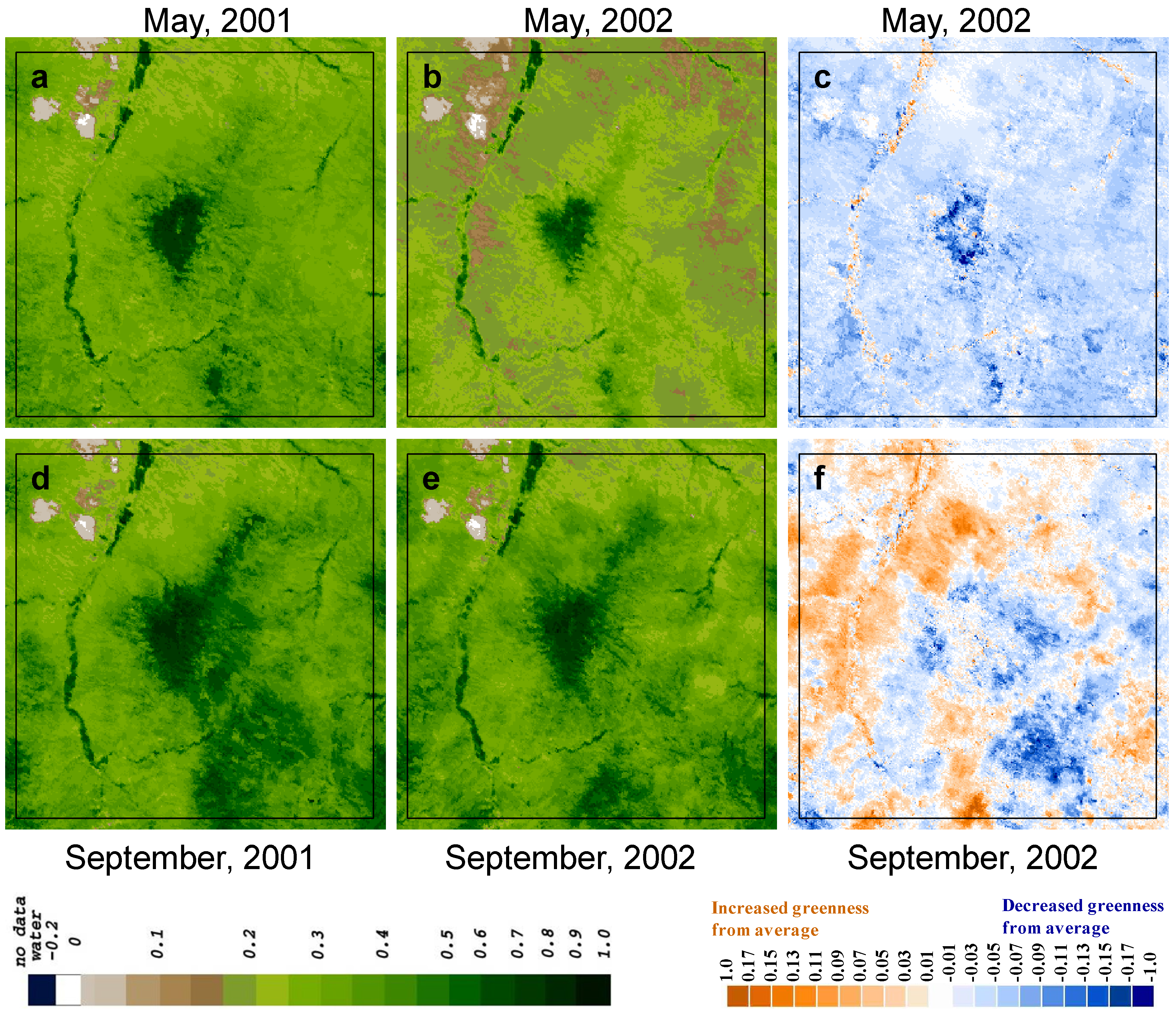
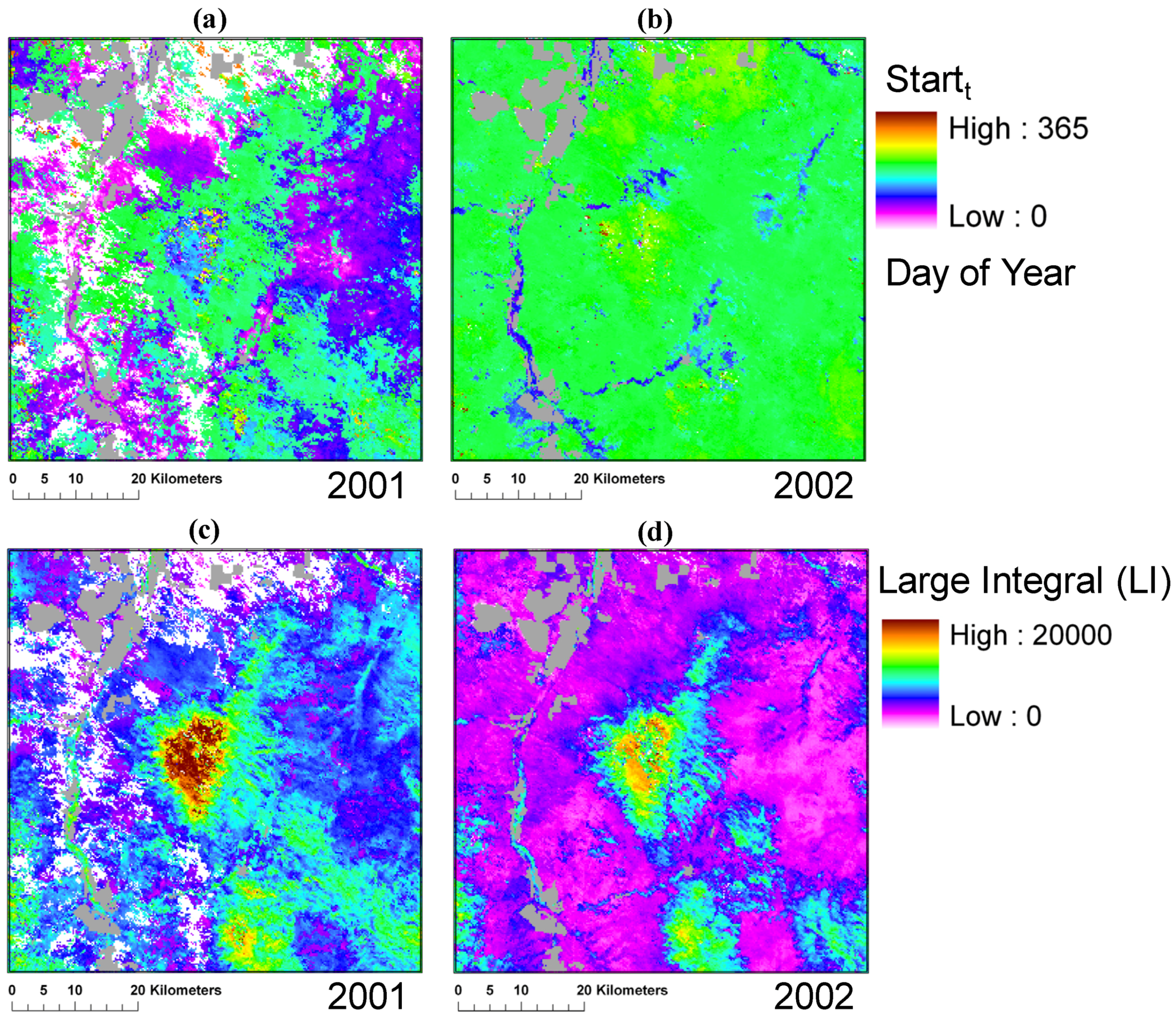
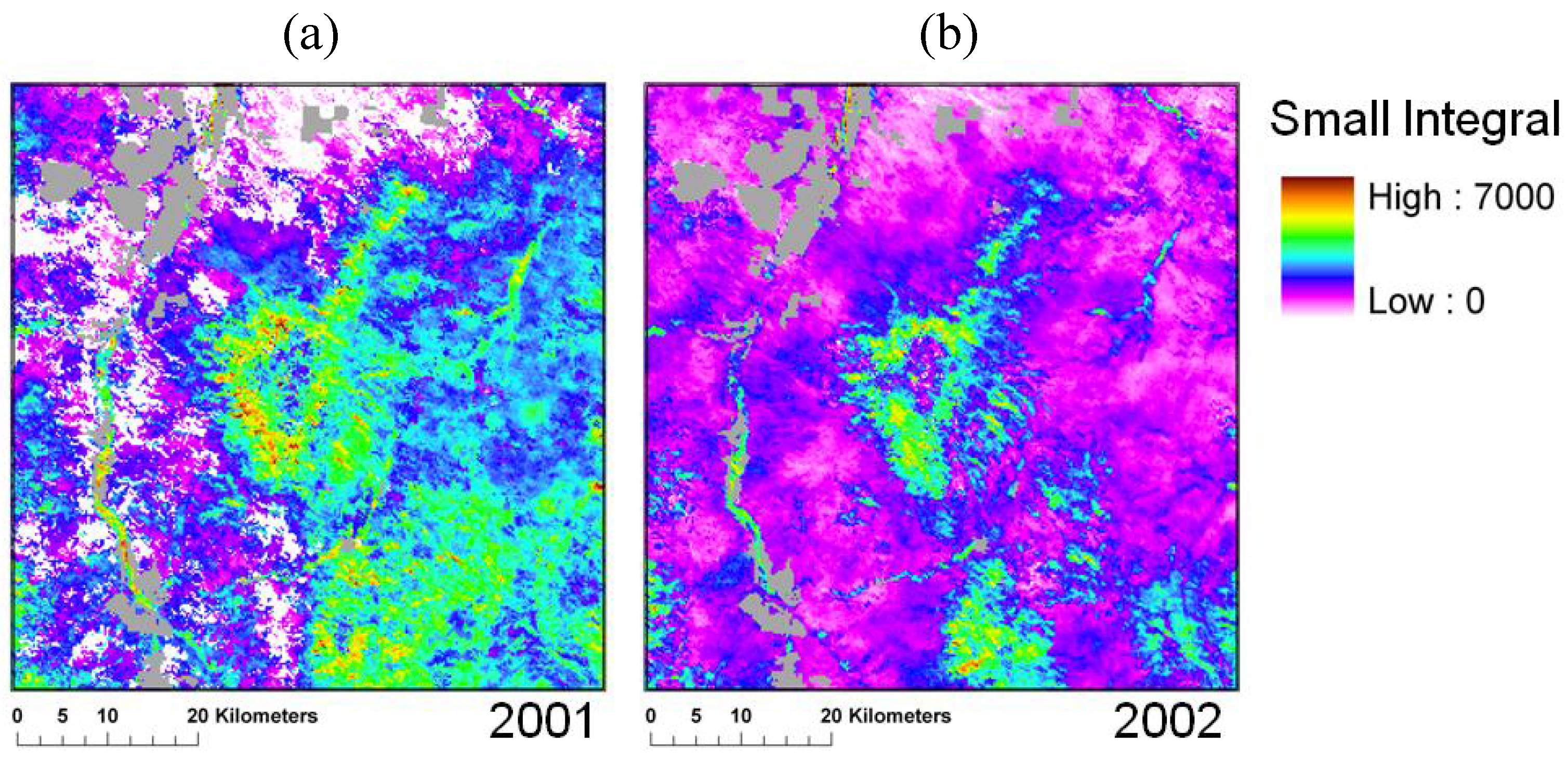
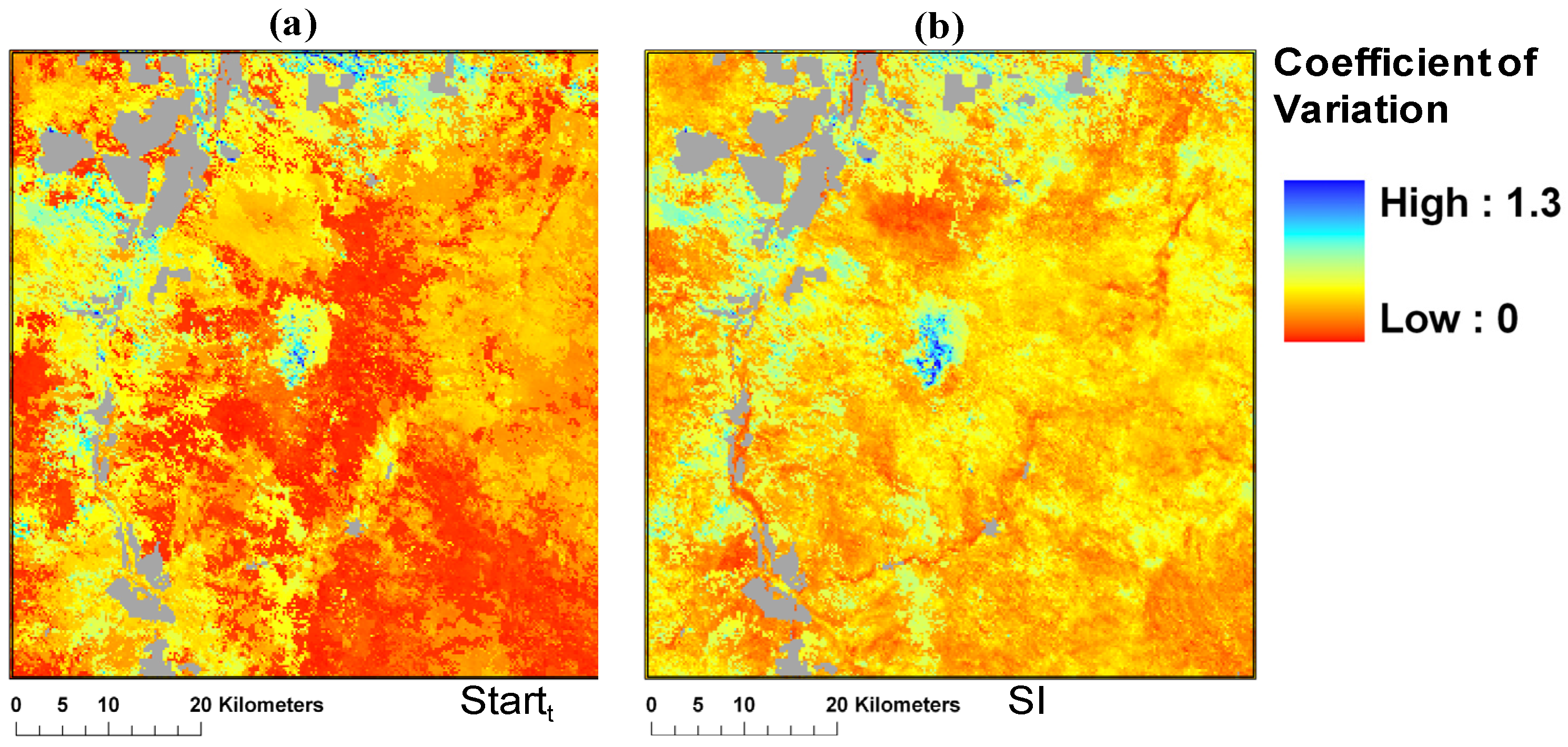
3.2. Spatio-Temporal Patterns of Phenometrics

Assessment of image-based spatial and temporal patterns of phenometrics revealed both spatial and temporal patterns (Figure 7, Figure 8 and Figure 9). The start of the growing season was comparatively spatially asynchronous in 2001 (Figure 7a) and synchronous in 2002 (Figure 7b).
Figure 7. Start of season (Startt; Day of Year) and for (a) 2001 and (b) 2002, and Large Integral for (c) 2001 and (d) 2002 across the Santa Rita Mountains, AZ. Gray areas are agricultural or industrial land cover types and are excluded from analysis while white areas represent incomplete phenological retrievals for that year.
Remotesensing 02 00388 g007
These patterns in synchronicities could be related to a bimodal growing season in 2001and a uni-modal growing season (skipped the spring due to the lack of precipitation) in 2002 for most vegetation communities. Annual integration of the NDVI values show that vegetation production was higher in 2001 (Figure 7c) than in 2002 (Figure 7d), and suggests the impact of inter-annual climate variability.
Interestingly, we observe that the seasonally integrated or small integral (Figure 8) is lower for the higher elevation vegetation cover types than the middle elevation cover types, suggesting more seasonally dynamic responses at these intermediate elevation levels. This might be attributed to the broadleaf deciduous woody plants (e.g., oak) at these elevations that senesce in the fall and winter, while higher-elevation coniferous vegetation communities keep their green plant matter.
Figure 8. Small NDVI integral for 2001 (a) and 2002 (b) shows both the seasonal response and spatial patterns for the vegetation cline. The mid elevation vegetation types have larger small NDVI integral values than the high elevation vegetation types and the desert vegetation types. Gray areas are agricultural or industrial land cover types and are excluded from analysis while white areas represent incomplete phenological retrievals.
Remotesensing 02 00388 g008
The observed spatial patterns in the COV for the Start of the season and Small Integral (Figure 9) suggest that the inter-annual variability in the start of season (Startt) and seasonal small integral (SI) responses are somewhat different across vegetation types and among phenometrics.
Figure 9. Spatial patterns of the coefficient of variation (COV) for the start of the season (SOS) (a) and the small NDVI integral (SI) (b) for 2001 through 2006.
Remotesensing 02 00388 g009
The effect of a forest fire in 2005 is also clearly visible at the top of the mountain range; this area was excluded from further analysis. Distinguishing phenological characteristics of vegetation types, including both their mean values and their variability, have been exploited in some land cover classifications [51,52], albeit at coarser biological and spatial scales than this study. Patterns shown in our phenometrics images suggest that classification might be a possibility at this spatial scale as well.

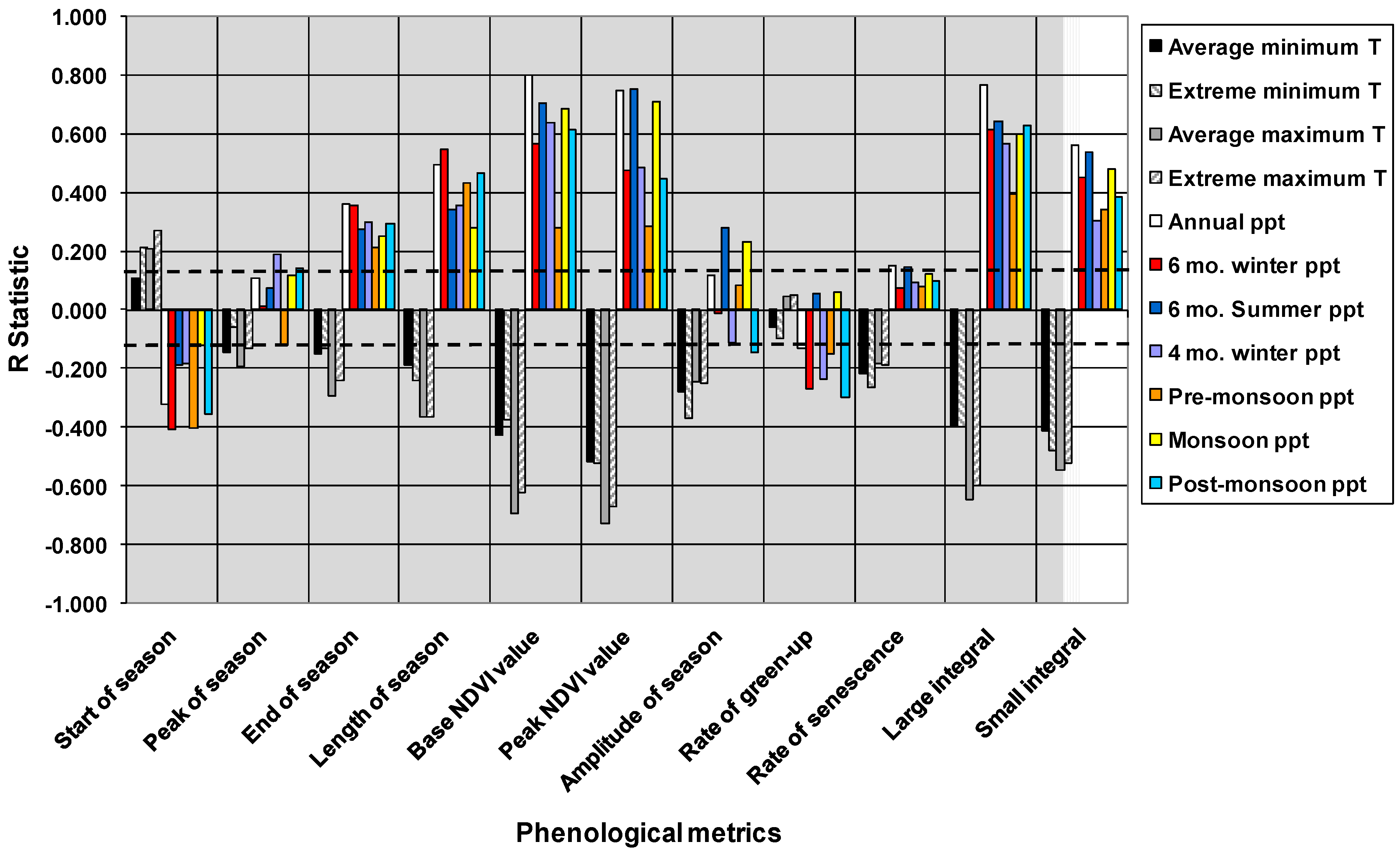
3.3. Phenometrics and Climate across Vegetation Communities

Phenometrics were highly correlated to many climate metrics in our analysis across vegetation types (Figure 10). Significant positive correlations to precipitation and negative correlations to temperature metrics were seen for many of the phenometrics describing the magnitude of seasons, such as BaseNDVI, amplitude, and large integral. Similar patterns have also been seen in global studies of NDVI as related to precipitation and temperature [53]. Linderman et al. [54] found that phenometrics varied across the African continent due to climate more than due to land use change.
Figure 10. Correlations among phenometrics and temperature (T) and precipitations (ppt) metrics, across vegetation types, Santa Rita Mountains, AZ, USA, 2001–2006. The dashed lines represent the threshold of p = 0.05, corresponding to |R| ≥ 0.1295.
Remotesensing 02 00388 g010
Correlations of timing metrics (start, peak, and end of season) with climate were less strong than correlations of many of the magnitude metrics, suggesting that there might be different causes than temperature and precipitation for variability in these phenometrics (e.g., soil and vegetation type, growing degree days) [2,55]. Across vegetation types an earlier start of season was correlated with lower temperatures and higher precipitation. Start of season showed negative correlations for precipitation and positive correlations for temperature (i.e., an earlier season start correlates with more rain and lower temperatures), while peak and end of season were shown to be later in the season with higher precipitation and lower temperatures.
Table 2. Results of stepwise regression of climate variables for each phenometric, for sites across the Santa Rita Mountains, AZ (n = 238; degrees of freedom listed with test statistics; R2 values are adjusted to account for multiple variables). Negative associations are indicated by italics. * = data were log transformed; ** = data were square-root transformed. Both transforms were made to improve the normal distribution of the data.
Pheno-metricExtreme minimum temp.Extreme maximum temp.Annual precip.Winter precip.*Pre-monsoon precip.**Monsoon precip.Post-monsoon precip.*Whole model
Start of season β = -2.25e-2β = 1.35 β = 2.81e-2 F3,234 = 24.6
t234 = -7.85t234 = 2.84t234 = 6.46p < 0.0001
p < 0.0001p = 0.0050p < 0.0001R2 = 0.230
Peak of season β = -2.02e-1 β = 7.26e-1β = -2.14e-1 F3,234 = 6.7
t234 = -2.53t234 = 2.24t234 = -3.57p = 0.002
p = 0.0122p = 0.0261p = 0.0004R2 = 0.067
End of season β = 1.00e-2 F1,236 = 34.8
t236 = 5.90p < 0.0001
p < 0.0001R2 = 0.125
Length of season β = 3.10e-2 β = -3.09e-2 F2,235 = 59.4
t235 = 10.27t235 = -5.74p < 0.0001
p < 0.0001p < 0.0001R2 = 0.330
Base NDVI* β = -7.45e-2β = 4.17e-3 β = -7.44e-2β = -3.31e-3β = -1.57e-1F5,232 = 127.9
t232 = -8.48t232 = 11.41t232 = -8.08t232 = -6.53t232 = -4.84p < 0.0001
p < 0.0001p < 0.0001p < 0.0001p < 0.0001p < 0.0001R2 = 0.744
Peak NDVI β = -1.68e-2β = -1.65e-2β = 9.78e-4 β = -1.11e-2 β = -8.10e-2F5,232 = 114.9
t232 = -4.35t232 = -4.18t232 = 13.86t232 = -5.15t232 = -7.06p < 0.0001
p < 0.0001p < 0.0001p < 0.0001p < 0.0001p < 0.0001R2 = 0.706
Amplitude of season β = -1.54e-2 β = -2.87e-4 β = 9.44e-3β = 7.71e-4β = -3.74e-2F4,233 = 24.2
t233 = -5.49t233 = -2.29t233 = 3.15t233 = 4.67t233 = -4.58p < 0.0001
p < 0.0001p = 0.0230p = 0.0019p < 0.0001p < 0.0001R2 = 0.328
Rate of Greenup β = -2.99e-4 β = 5.32e-3β = 4.95e-4 F3,234 = 20.4
t234 = -7.31t234 = 4.39t234 = 7.37p < 0.0001
p < 0.0001p < 0.0001p < 0.0001R2 = 0.197
Rate of Senescence* β = -9.64e-2 F1,236 = 22.4
t236 = -4.74p < 0.0001
p < 0.0001R2 = 0.083
Small Integral* β = 9.49e-2 β = 1.98e-3 β = 1.68e-1F3,234 = 62.47
t234 = -6.89t234 = 8.03t234 = -3.65p < 0.0001
p < 0.0001p < 0.0001p = 0.0003R2 = 0.438
Large Integral*β = -4.11e-2β = -3.54e-2β = 2.35e-3 F2,234 = 127.6
t234 = -2.76t234 = -2.35t234 = 11.07p < 0.0001
p = 0.0063p = 0.0197p < 0.0001R2 = 0.616
As the Southwest was in a drought for most of our study period (2002 through 2005 and ongoing), accompanied by anomalously warm temperatures at least in the worst drought year (2002) [16], relationships showing dependence on water and cooler temperatures are not surprising [56]. Increased precipitation could delay plant senescence and therefore the peak and end of the growing season. Lower temperatures might allow plants to continue to photosynthesize due to lessened vapor pressure deficit or other factors affecting drought stress [16,40]. Also, these patterns might highlight the dominance of the lower-elevation desert vegetation types in our study area, communities which experience less low-temperature-limitations, except in the winter.
Stepwise regression for each metric likewise showed salient relationships between metrics and climate (Table 2). Each phenometric showed moderate to highly significant relationships with climate metrics, and the combination of relationships was unique per metric. The amount of variation in phenometrics that was explained by climate metrics varied from less than seven percent to over 74% (adjusted R2; Table 2). BaseNDVI, peakNDVI and large integral were best explained by climate metrics, while peak and end dates and rates of green-up and senescence were not well explained by climate metrics across all sample sites. Annual precipitation explained variation in almost all phenometrics.

3.4. Phenometrics and Climate by Vegetation Type

Analysis of phenometrics by vegetation type (11) showed correlations between both timing- and magnitude-based phenometrics and climate metrics. Correlations of a high and low elevation vegetation community are shown in Table 3 and Table 4 respectively, while an overview of all significant relationships for all 11 vegetation types are provided in Appendix A. After a Bonferroni adjustment for multiple comparisons, 121 tests (11 phenometrics × 11 climate variables) and a mean correlation of 0.62 [57], lowering the alpha from 0.05 to 0.0081 for each test, 128 pheno-climate relationships were significantly correlated (p ≤ 0.0081). Of these 128 relationships between phenometrics and climate metrics, 88 were related to precipitation metrics and 40 to temperature metrics. Another 198 pheno-climate relationships were significantly correlated at 0.0081 < p ≤ 0.05 (without Bonferroni adjustments; data not shown). Of these 198 relationships between phenometrics and climate metrics, 118 were related to precipitation metrics and 70 to temperature metrics. The pheno-climate relationships are dominated by precipitation metrics (66%), although temperature metrics also plays a considerable role (34%) among these. Negative correlations were found for 124 out of the 326 total pheno-climate relationships which were evenly distributed between temperature and precipitation metrics, but about 65% of these were related to timing based phenometrics. An overview of the number of significant pheno-climate relationships across all vegetation types by phenometric and climate metric is provided in Appendix B. This overview suggests that some of the phenometrics, like the end of the season and rate of green-up are not as often correlated to climate metrics as some of the other phenometrics. It also suggests that precipitation-based metrics are relatively more important than temperature-based metrics for this gradient, while the winter precipitation (4 mo.) has the fewest number of significant relationships.
As in our analysis across vegetation types, magnitude-based metrics were often positively correlated with precipitation and negatively correlated with temperature. Significant relationships were found in all of the vegetation communities. Correlation matrices suggested unique relationships between phenometrics and climate metrics for each community along the elevation gradient (data shown in Appendix A). For example, in the pine-oak woodland vegetation community, most phenometrics were correlated with precipitation metrics and not with any of the temperature metrics (Table 3). The base, peak and integrated NDVI metrics were positively correlated with several precipitation metrics (i.e., winter, pre-monsoon and annual precipitation), while most of the timing based phenometrics were negatively correlated with several of the precipitation metrics. For example, an earlier start of the growing season was a function of both pre- and post-monsoon precipitation, indicating that soil moisture accumulation during fall and winter will result in an earlier start of the next spring or summer growing season. The rate of senescence is slower when we have winter precipitation.
Table 3. Significant correlations (p ≤ 0.0081) between phenometrics and climate metrics for pine-oak woodland. Relationships that have negative R values are italicized. (Elevation ~2,204 m).
PhenometricClimate MetricRp-valuen
Base NDVI valueWinter (6 mo) precipitation0.620.000527
Base NDVI valueAnnual precipitation0.500.007627
End of seasonMonsoon precipitation−0.510.006127
Large integralWinter (6 mo) precipitation0.630.000427
Large integralPre-monsoon precipitation0.610.000627
Length of seasonPre-monsoon precipitation0.640.000327
Peak NDVI valueWinter (6 mo) precipitation0.670.000127
Peak NDVI valueAnnual precipitation0.520.005327
Rate of senescenceWinter(6 mo) precipitation−0.540.003727
Small integralPre-monsoon precipitation0.550.002927
Start of seasonPost-monsoon precipitation−0.530.004427
Start of seasonPre-monsoon precipitation−0.640.000427
In contrast, in the grassland community (Table 4) a later start of season was correlated with extreme maximum and minimum temperatures, while an earlier start of the season was correlated with more winter and pre-monsoon precipitation. The peak of season is earlier with more pre-monsoon, annual and winter precipitation and lower maximum temperatures. The end of season seems to be later with higher average minimum and maximum temperatures, suggesting that these temperatures extend the growing season. It is less evident why less winter precipitation would result in a later end of the growing season. More complex temperature, precipitation and environmental feedback mechanisms and interactions would need to be explored further. Most magnitude based metrics like SI, LI, NDVIpeak, and NDVIbase increase with precipitation metrics (e.g., summer, annual, and winter precipitation), and decrease with extreme low or high temperatures.
While some of the magnitude-based phenometrics correlated similarly to climate metrics for many vegetation types, correlations of timing-based phenometrics seemed more inconsistent between vegetation types. It could be that the timing of plant growth cycles is more variable than magnitude on a landscape scale. DeFries et al. [51] found that vegetation types were distinguished from one another using unique metrics for each separation; our study suggests the same. Heumann et al. [58] found that different TIMESAT-derived phenometrics responded to climate factors in different regions; similar patterns are illustrated in this research by the ability to distinguish vegetation communities across this steep climatic gradient that represents many ecoregions. As individual plants respond directly to soil moisture patterns rather than rain or snow per se [59], highly variable timing might be related to soil type and texture, as well as plant functional type [60], topography, or antecedent precipitation [59,61]. And finally, with the studied landscape also experiencing drought it might be expected to display vegetation phenology that is highly sensitive to precipitation pulses and therefore potentially quite spatially heterogeneous [56,59,62].
Table 4. Significant correlations (p ≤ 0.0081) between phenometrics and climate metrics for semi-desert grassland. Relationships that have negative R values are italicized. (Elevation ~1,357 m).
PhenometricClimate MetricRp-valuen
Amplitude of seasonSummer precipitation0.590.002823
Base NDVI valueAnnual precipitation0.740.000123
Base NDVI valueWinter (6 mo) precipitation0.580.004123
Base NDVI valueAverage maximum temperature−0.600.002523
End of seasonAverage minimum temperature0.640.001023
End of seasonAverage maximum temperature0.640.001123
End of seasonWinter (6 mo) precipitation−0.590.003023
Large integralAnnual precipitation0.730.000123
Large integralSummer precipitation0.700.000223
Large integralPre-monsoon precipitation0.580.003423
Large integralExtreme maximum temperature−0.540.007223
Large integralExtreme minimum temperature−0.630.001323
Length of seasonPre-monsoon precipitation0.620.001523
Peak NDVI valueSummer precipitation0.640.001023
Peak of seasonAverage maximum temperature0.540.008023
Peak of seasonPre-monsoon precipitation−0.600.002723
Peak of seasonAnnual precipitation−0.720.000123
Peak of seasonWinter(6 mo) precipitation−0.740.000023
Small integralSummer precipitation0.750.000023
Small integralAnnual precipitation0.590.003123
Small integralMonsoon precipitation0.560.005523
Start of seasonExtreme maximum temperature0.590.003023
Start of seasonExtreme minimum temperature0.550.006723
Start of seasonWinter (6 mo) precipitation−0.560.005423
Start of seasonPre-monsoon precipitation−0.610.002223
In addition to limitations in spatial resolution, the temporal resolution of the standard 16-day NDVI data products could potentially also preclude a more precise capture of vegetation community phenology; certain growth phases can be overlooked within a 16-day period [1,63], although most timing-based metrics tend to be within 3 days when based on 16-day composited MODIS time series data [64]. Use of more finely resolved and cloud-free time series data might provide more precise phenology and could positively or negatively affect the relationships between phenology and other environmental factors. Finally, the algorithms or the settings used in TIMESAT could be optimized for each vegetation type, possibly resulting in slightly different metrics of the phenology for each of these communities. However, tracking the optimal setting for each pixel might not be practical and could lead to less spatially and temporally consistent phenometrics.

4. Conclusions

Use of phenometrics to describe vegetation response to climate trends and variability across a sky island, with the finer spatial resolution of the Moderate Resolution Imaging Spectroradiometer (MODIS) Normalized Difference Vegetation Index (NDVI) at 250 m and 16-day composite intervals, allows for a more detailed look at the vegetation communities in and around steep biological gradients than current phenology studies typically employ [13,35,65]. The temporal and spatial heterogeneity in land surface phenological patterns along this climate and elevation gradient were well characterized and depicted by phenometric images and examples of COV images for the start of season and small NDVI integral. Examples of spatial patterns in land surface phenometrics showed that the start of the growing season and annual productivity for the 11 vegetation communities are highly variable between years. Example COV images provided an important spatial representation of the distinct interannual variability among phenometrics.
This phenoclimatological study provides the groundwork and support for our hypotheses. Remotely sensed phenological signatures and phenometrics differed across the elevation gradient and were unique for each vegetation type. Most vegetation types (11) and associated phenometrics (11) showed distinct relationships and significant correlations (128 relationships, p ≤ 0.0081, Appendix A; 326 relationships, p ≤ 0.05, Appendix B) for many of the seven precipitation and four temperature metrics. The climate metrics were less successful in explaining variability in each of the phenometrics across all sample sites at once (representing all 11 vegetation community types). This suggests that some phenological similarities exist across the elevation gradient, but that most of the variability among vegetation type communities could not be fully captured by the generalized pheno-climate models created in this study (Table 2).
Low-elevation desert sites (e.g., creosote, palo verde and mesquite communities) had seasonal shapes that included sharp seasonal peaks in NDVI and slight to strong bimodality. These features might point to the potentially high degree of sensitivity of these communities to precipitation events [1,49]. Additionally, inter-annual variation might be related to temperature; low temperatures might postpone the start of the growing season in the spring, especially at higher elevations, while high temperatures might result in high evapotranspiration rates, possibly postponing the onset of the growing season or reducing the vigor and possibly the length of the growing season, especially in the lower elevations where shallow rooted herbaceous plants and shrubs are more water limited than plants at higher elevations.
Spatial and temporal resolution of the MODIS and PRISM data might have hindered more precise relationships, but our study demonstrates the value of these datasets in exploring landscape-scale phenology across steep elevation and linked biological gradients. The number of observations could be augmented and the results made more ecologically robust by including more samples from other Sky Islands. Environmental factors beside climate, such as topography (slope and aspect) and soil physical and chemical properties (water permeability, surface rock fragments, soil depth, carbon, and nutrient availability) might contribute the phenological changes as well and could be a focus of future research. Impacts of pulse driven and lagged land surface phenological response to climate variables can also be further explored, especially if we examine sky island resilience to changes.
Use of phenometrics in this manner could be helpful in updating land cover classifications over seasons [66]. Monitoring ecotones and transition zones of sky islands could be practical for management and conservation purposes, and further development of the presented methods could result in tools for such monitoring. Additionally, sky islands could be used as indicators and barometers of stress [28]. Sky islands provide the ability to do this, as they represent a latitudinal gradient as well as many of the US Southwest’s dominant vegetation types within a relatively small area. Continuing research into the spatio-temporal phenological patterns of sky islands could assist in the conservation of these areas as biodiversity hotspots. Additionally, mapping of vegetation communities based on phenology could allow for the accounting of interannual and seasonal landscape-scale community responses to interacting environmental factors [67].

Acknowledgements

MODIS data were distributed by the Land Processes Distributed Active Archive Center (LP DAAC), located at the U.S. Geological Survey, Earth Resources Observation and Science (EROS) http://lpdaac.usgs.gov. The authors appreciate to use of the TIMESAT software, made available by Per Jönsson and Lars Eklundh.

References

  1. Reed, B.C.; Brown, J.F.; Vanderzee, D.; Loveland, T.R.; Merchant, J.W.; Ohlen, D.O. Measuring phenological variability from satellite imagery. J. Veg. Sci. 1994, 5, 703–714. [Google Scholar] [CrossRef]
  2. Schwartz, M.D. Monitoring global change with phenology: the case of the spring green wave. Int. J. Biometeorol. 1994, 38, 18–22. [Google Scholar] [CrossRef]
  3. Justice, C.O.; Townshend, J.R.G.; Holben, B.N.; Tucker, C.J. Analysis of the phenology of global vegetation using meteorological satellite data. Int. J. Remote Sens. 1985, 6, 1271–1318. [Google Scholar] [CrossRef]
  4. Tucker, C.J. Red and photographic infrared linear combinations for monitoring vegetation. Remote Sens. Environ. 1979, 8, 127–150. [Google Scholar] [CrossRef]
  5. Nemani, R.; Keeling, C.; Hashimoto, H.; Jolly, W.; Piper, S.; Tucker, C.; Myneni, R.; Running, S. Climate driven increases in global terrestrial net primary production from 1982–1999. Science 2003, 300, 1562–1563. [Google Scholar] [CrossRef] [PubMed]
  6. Goward, S.N.; Tucker, C.J.; Dye, D.G. North American vegetation patterns observed with the NOAA-7 advanced very high resolution radiometer. Plant Ecol. 1985, 64, 3–14. [Google Scholar] [CrossRef]
  7. Baret, F.; Guyot, G. Potentials and limits of vegetation indices for LAI and APAR assessment. Remote Sens. Envion. 1991, 35, 161–173. [Google Scholar] [CrossRef]
  8. Colwell, J.E. Vegetation Canopy Reflectance. Remote Sens. Environ. 1974, 3, 175–183. [Google Scholar] [CrossRef]
  9. Parmesan, C.; Yohe, G. A globally coherent fingerprint of climate change impacts across natural systems. Nature 2003, 421, 37–42. [Google Scholar] [CrossRef] [PubMed]
  10. Myneni, R.B.; Keeling, C.D.; Tucker, C.J.; Asrar, G.; Nemani, R.R. Increased plant growth in the northern high latitudes from 1981–1991. Nature 1997, 386, 698–702. [Google Scholar] [CrossRef]
  11. White, M.A.; Hoffman, F.; Hargrove, W.W.; Nemani, R.R. A global framework for monitoring phenological responses to climate change. Geophys. Res. Lett. 2005, 32, 1–4. [Google Scholar] [CrossRef]
  12. Gao, Y.; Mas, J.F.; Navarrete, A. The improvement of an object-oriented classification using multi-temporal MODIS EVI satellite data. Int. J. Dig. Earth 2009, 2, 219–236. [Google Scholar] [CrossRef]
  13. White, M.A.; de Beurs, K.M.; Didan, K.; Inouye, D.W.; Richardson, A.D.; Jensen, O.P.; O'Keefe, J.; Zhang, G.; Nemani, R.R.; van Leeuwen, W.J.D.; Brown, J.F.; de Wit, A.; Schaepman, M.; Lin, X.M.; Dettinger, M.; Bailey, A.S.; Kimball, J.; Schwartz, M.D.; Baldocchi, D.D.; Lee, J.T.; Lauenroth, W.K. Intercomparison, interpretation, and assessment of spring phenology in North America estimated from remote sensing for 1982–2006. Glob. Change Biol. 2009, 15, 2335–2359. [Google Scholar] [CrossRef]
  14. van Leeuwen, W.J.D. Monitoring the effects of forest restoration treatments on post-fire vegetation recovery with MODIS multitemporal data. Sensors 2008, 8, 2017–2042. [Google Scholar] [CrossRef]
  15. Hwang, T.; Kangw, S.; Kim, J.; Kim, Y.; Lee, D.; Band, L. Evaluating drought effect on MODIS Gross Primary Production (GPP) with an eco-hydrological model in the mountainous forest, East Asia. Glob. Change Biol. 2008, 14, 1037–1056. [Google Scholar] [CrossRef]
  16. Breshears, D.D.; Cobb, N.S.; Rich, P.M.; Price, K.P.; Allen, C.D.; Balice, R.G.; Romme, W.H.; Kastens, J.H.; Floyd, M.L.; Belnap, J.; Anderson, J.J.; Myers, O.B.; Meyer, C.W. Regional vegetation die-off in response to global-change-type drought. Proc. Nat. Acad. Sci. USA 2005, 102, 15144–15148. [Google Scholar] [CrossRef] [PubMed]
  17. White, M.A.; Nemani, R.R.; Thornton, P.E.; Running, S.W. Satellite evidence of phenological differences between urbanized and rural areas of the eastern United States deciduous broadleaf forest. Ecosystems 2002, 5, 260–273. [Google Scholar] [CrossRef]
  18. de Beurs, K.M.; Henebry, G.M. Land surface phenology, climatic variation, and institutional change: Analyzing agricultural land cover change in Kazakhstan. Remote Sens. Environ. 2004, 89, 497–509. [Google Scholar] [CrossRef]
  19. Reed, B.C.; White, M.; Brown, J.F. Remote Sensing Phenology; Kluwer Academic Publishers: Dordrecht, the Netherlands, 2003; pp. 365–381. [Google Scholar]
  20. Jönsson, P.; Eklundh, L. Seasonality extraction and noise removal by function fitting to time-series of satellite sensor data. IEEE Trans. Geosci. Remot. Sen. 2002, 40, 1824–1832. [Google Scholar] [CrossRef]
  21. Jönsson, P.; Eklundh, L. TIMESAT–a program for analyzing time-series of satellite sensor data. Comput. Geosci. 2004, 30, 833–845. [Google Scholar] [CrossRef]
  22. Warshall, P. The Madrean sky island archipelago: a planetary overview. In Biodiversity and management of the Madrean Archipelago: the Sky Islands of Southwestern United States and Northwestern Mexico; DeBano, F.L., Ffolliott, P.F., Ortega-Rubio, A., Gottfried, G.J., Hamre, R.H., Edminster, C.B., Eds.; General Technical Report RM-GTR-264; US Department of Agriculture, Forest Service: Fort Collins, CO, USA, 1994; pp. 408–415. [Google Scholar]
  23. Coblentz, D.D.; Riitters, K.H. Topographic controls on the regional-scale biodiversity of the south-western USA. J Biogeogr. 2004, 31, 1125–1138. [Google Scholar] [CrossRef]
  24. Madrean Pine-Oak Woodlands—Biodiversity Hotspots. Conservation International. Available online: http://www.biodiversityhotspots.org/xp/hotspots/pine_oak/Pages/biodiversity.aspx (accessed on October 12, 2009).
  25. Swetnam, T.W.; Baisan, C.H. Historical Fire Regime Patterns in the Southwestern United States since AD 1700; USDA Forest Service: Fort Collins, CO, USA, 1996; pp. 11–32. [Google Scholar]
  26. Westerling, A.L.; Hidalgo, H.G.; Cayan, D.R.; Swetnam, T.W. Warming and earlier spring increase western US forest wildfire activity. Science 2006, 313, 940–943. [Google Scholar] [CrossRef] [PubMed]
  27. Impacts, Adaptation and Vulnerability: Summary for Policymakers; IPCC Climate Change 2007; Intergovernmental Panel on Climate Change: Brussels, Belgium, 2007; pp. 1–23.
  28. NEON Report on first Workshop on the National Ecological Observatory Network (NEON); Archbold Biological Station: Lake Placid, FL, USA, 2000.
  29. DeLong, J.P.; Cox, S.W.; Cox, N.S. A comparison of avian use of high- and low-elevation sites during autumn migration in central New Mexico. J. Field Ornithol. 2005, 76, 326–333. [Google Scholar] [CrossRef]
  30. Alerstam, T.; Hedenstrom, A. The development of bird migration theory. J. Avian Biology 1998, 29, 343–369. [Google Scholar] [CrossRef]
  31. Brown-Mitic, C.; Shuttleworth, W.J.; Chawn Harlow, R.; Petti, J.; Burke, E.; Bales, R. Seasonal water dynamics of a sky island subalpine forest in semi-arid southwestern United States. J. Arid Environ. 2007, 69, 237–258. [Google Scholar] [CrossRef]
  32. Marshall, J.T. Birds of the Pine-Oak Woodland in Southern Arizona and Adjacent Mexico; Cooper Ornithological Society: Berkeley, CA, USA, 1957; p. 125. [Google Scholar]
  33. Whittaker, R.H.; Niering, W.A. Vegetation of Santa Catalina Mountains, Arizona. 5. Biomass, production, and diversity along the elevation gradient. Ecology 1975, 56, 771–790. [Google Scholar] [CrossRef]
  34. Merriam, C.H.; Steineger, L. Results of a Biological Survey of the San Francisco Mountain Region and the Desert of the Little Colorado, Arizona; North American Fauna Report 3; US Department of Agriculture, Division of Ornithology and Mammalogy: Washington, DC, USA, 1890; pp. 1–136. [Google Scholar]
  35. Moulin, S.; Kergoat, L.; Viovy, N.; Dedieu, G. Global-scale assessment of vegetation phenology using NOAA/AVHRR satellite measurements. J. Climate 1997, 10, 1154–1170. [Google Scholar] [CrossRef]
  36. Justice, C.O.; Vermote, E.; Townshend, J.R.G.; Defries, R.; Roy, D.P.; Hall, D.K.; Salomonson, V.V.; Privette, J.L.; Riggs, G.; Strahler, A.; Lucht, W.; Myneni, R.B.; Knyazikhin, Y.; Running, S.W.; Nemani, R.R.; Wan, Z.M.; Huete, A.R.; van Leeuwen, W.; Wolfe, R.E.; Giglio, L.; Muller, J.P.; Lewis, P.; Barnsley, M.J. The Moderate Resolution Imaging Spectroradiometer (MODIS): Land remote sensing for global change research. IEEE Trans. Geosci. Remote Sens. 1998, 36, 1228–1249. [Google Scholar] [CrossRef]
  37. Huete, A.; Didan, K.; Miura, T.; Rodriguez, E.P.; Gao, X.; Ferreira, L.G. Overview of the radiometric and biophysical performance of the MODIS vegetation indices. Remote Sens. Environ. 2002, 83, 195–213. [Google Scholar] [CrossRef]
  38. Casady, G.M.; van Leeuwen, W.J.D.; Marsh, S.E. Evaluation post-wildfire vegetation regeneration as a response to multiple environmental determinants. Environ. Model. Assess. 2010, in press. [Google Scholar] [CrossRef]
  39. van Leeuwen, W.J.D.; Casady, G.M.; Neary, D.G.; Bautista, S.; Alloza, J.A.; Carmel, Y.; Wittenberg, L.; Malkinson, D.; Orr, B.J. Monitoring post-wildfire vegetation response with remotely sensed time-series data in Spain, USA and Israel. Int. J. Wildland Fire 2010, in press. [Google Scholar] [CrossRef]
  40. White, M.A.; Thornton, P.E.; Running, S.W. A continental phenology model for monitoring vegetation responses to interannual climatic variability. Global Biogeochem. Cycle. 1997, 11, 217–234. [Google Scholar] [CrossRef]
  41. Bradley, B.A.; Jacob, R.W.; Hermance, J.F.; Mustard, J.F. A curve fitting procedure to derive inter-annual phenologies from time series of noisy satellite NDVI data. Remote Sens. Environ. 2007, 106, 137–145. [Google Scholar] [CrossRef]
  42. Morisette, J.T.; Richardson, A.D.; Knapp, A.K.; Fisher, J.I.; Graham, E.A.; Abatzoglou, J.; Wilson, B.E.; Breshears, D.D.; Henebry, G.M.; Hanes, J.M.; Liang, L. Tracking the rhythm of the seasons in the face of global change: phenological research in the 21st century. Front. Ecol. Environ. 2009, 7, 253–260. [Google Scholar] [CrossRef]
  43. Crimmins, T.M.; Crimmins, M.A.; Bertelsen, C.D. Flowering range changes across an elevation gradient in response to warming summer temperatures. Glob. Change Biol. 2009, 15, 1141–1152. [Google Scholar] [CrossRef]
  44. Lowry, J.; Ramsey, R.D.; Thomas, K.; Schrupp, D.; Sajwaj, T.; Kirby, J.; Waller, E.; Schrader, S.; Falzarano, S.; Langs, L.; Manis, G.; Wallace, C.; Schulz, K.; Comer, P.; Pohs, K.; Rieth, W.; Velasquez, C.; Wolk, B.; Kepner, W.; Boykin, K.; O'Brien, L.; Bradford, D.; Thompson, B.; Prior-Magee, J. Mapping moderate-scale land-cover over very large geographic areas within a collaborative framework: a case study of the Southwest Regional Gap Analysis Project (SWReGAP). Remote Sens. Environ. 2007, 108, 59–73. [Google Scholar] [CrossRef]
  45. Huete, A.R.; Liu, H.Q.; Batchily, K.; van Leeuwen, W.J.D. A comparison of Vegetation Indices over a Global Set of TM images for EOS-MODIS. Remote Sens. Environ. 1997, 59, 440–451. [Google Scholar] [CrossRef]
  46. DiLuzio, M.; Johnson, G.L.; Daly, C.; Eischeid, J.K.; Arnold, J.G. Constructing retrospective gridded daily precipitation and temperature datasets for the conterminous United States. J. Appl. Meteorol. Climatol. 2008, 47, 475–497. [Google Scholar] [CrossRef]
  47. Crimmins, M.A.; Comrie, A.C. Interactions between antecedent climate and wildfire variability across south-eastern Arizona. Int. J. Wildland Fire 2004, 13, 455–466. [Google Scholar] [CrossRef]
  48. Richardson, A.D.; Braswell, B.H.; Hollinger, D.Y.; Jenkins, J.P.; Ollinger, S.V. Near-surface remote sensing of spatial and temporal variation in canopy phenology. Ecol. Appl. 2009, 19, 1417–1428. [Google Scholar] [CrossRef] [PubMed]
  49. Jackson, R.B.; Canadell, J.; Ehleringer, J.R.; Mooney, H.A.; Sala, O.E.; Schulze, E.D. A global analysis of root distributions for terrestrial biomes. Oecologia 1996, 108, 389–411. [Google Scholar] [CrossRef]
  50. Theresa, M.C.; Michael, A.C.; Bertelsen, C.D. Flowering range changes across an elevation gradient in response to warming summer temperatures. Glob. Change Biol. 2009, 15, 1141–1152. [Google Scholar]
  51. DeFries, R.; Hansen, M.; Townshend, J. Global discrimination of land cover types from metrics derived from AVHRR pathfinder data. Remote Sens. Environ. 1995, 54, 209–222. [Google Scholar] [CrossRef]
  52. Weiss, J.L.; Gutzler, D.S.; Coonrod, J.E.A.; Dahm, C.N. Long-term vegetation monitoring with NDVI in a diverse semi-arid setting, central New Mexico, USA. J. Arid Environ. 2004, 58, 249–272. [Google Scholar] [CrossRef]
  53. Schultz, P.A.; Halpert, M.S. Global correlation of temperature, NDVI and precipitation. Adv. Space Res. 1993, 13, 277–280. [Google Scholar] [CrossRef]
  54. Linderman, M.; Rowhani, P.; Benz, D.; Serneels, S.; Lambin, E.F. Land-cover change and vegetation dynamics across Africa. J. Geophys. Res.-Atmos. 2005, 110, D12. [Google Scholar] [CrossRef]
  55. Walther, G.R.; Post, E.; Convey, P.; Menzel, A.; Parmesan, C.; Beebee, T.J.C.; Fromentin, J.M.; Hoegh-Guldberg, O.; Bairlein, F. Ecological responses to recent climate change. Nature 2002, 416, 389–395. [Google Scholar] [CrossRef] [PubMed]
  56. Noy-Meir, I. Desert ecosystems: environment and producers. Ann. Rev. Ecol. Syst. 1973, 4, 25–52. [Google Scholar] [CrossRef]
  57. Sankoh, A.J.; Huque, M.F.; Dubey, S.D. Some comments on frequently used multiple endpoint adjustments methods in clinical trials. Stat. Med. 1997, 16, 2529–2542. [Google Scholar] [CrossRef]
  58. Heumann, B.W.; Seaquist, J.W.; Eklundh, L.; Jonsson, P. AVHRR derived phenological change in the Sahel and Soudan, Africa, 1982-2005. Remote Sens. Environ. 2007, 108, 385–392. [Google Scholar] [CrossRef]
  59. Loik, M.E.; Breshears, D.D.; Lauenroth, W.K.; Belnap, J. A multi-scale perspective of water pulses in dryland ecosystems: climatology and ecohydrology of the western USA. Oecologia 2004, 141, 269–281. [Google Scholar] [CrossRef] [PubMed]
  60. Archibald, S.; Scholes, R.J. Leaf green-up in a semi-arid African savanna–separating tree and grass responses to environmental cues. J. Veg. Sci. 2007, 18, 583–594. [Google Scholar] [CrossRef]
  61. Reynolds, J.F.; Kemp, P.R.; Ogle, K.; Fernandez, R.J. Modifying the ‘pulse-reserve’ paradigm for deserts of North America: precipitation pulses, soil water, and plant responses. Oecologia 2004, 141, 194–210. [Google Scholar] [CrossRef] [PubMed]
  62. Ignace, D.D.; Huxman, T.E.; Weltzin, J.F.; Williams, D.G. Leaf gas exchange and water status responses of a native and non-native grass to precipitation across contrasting soil surfaces in the Sonoran Desert. Oecologia 2007, 152, 401–413. [Google Scholar] [CrossRef] [PubMed]
  63. Schwartz, M.D.; Reed, B.; White, M.A. Assessing satellite-derived start-of-season (SOS) measures in the conterminous USA. Int. J. Climatol. 2002, 22, 1793–1805. [Google Scholar] [CrossRef]
  64. Zhang, X.; Friedl, M.; Schaaf, C. Sensitivity of vegetation phenology detection to the temporal resolution of satellite data. Int. J. Remote Sens. 2009, 30, 2061–2074. [Google Scholar] [CrossRef]
  65. Zhang, X.Y.; Friedl, M.A.; Schaaf, C.B.; Strahler, A.H.; Hodges, J.C.F.; Gao, F.; Reed, B.C.; Huete, A. Monitoring vegetation phenology using MODIS. Remote Sens. Environ. 2003, 84, 471–475. [Google Scholar] [CrossRef]
  66. Knight, J.F.; Lunetta, R.S.; Ediriwickrema, J.; Khorrarn, S. Regional scale land cover characterization using MODIS-NDVI 250 m multi-temporal imagery: a phenology-based approach. GISci. Remote Sens. 2006, 43, 1–23. [Google Scholar] [CrossRef]
  67. Loveland, T.R.; Merchant, J.W.; Brown, J.F.; Ohlen, D.O.; Reed, B.C.; Olson, P.; Hutchinson, J. Seasonal land-cover regions of the United States. Ann. Assn. Amer. Geogr. 1995, 85, 339–355. [Google Scholar] [CrossRef]

Appendix A

Significant (p ≤ 0.0081) correlations between phenometrics and climate variables for all dominant vegetation types along the elevation gradient in the Santa Rita Mountains, AZ, USA.
Veetation communityPhenometricClimate variableCorrelation (R)p-valuenElevation (m)
Conifer-oak forestPeak NDVI valueWinter precipitation (6 mo)0.900.0000152626
Conifer-oak forestBase NDVI valueWinter precipitation (6 mo)0.870.0000152626
Conifer-oak forestPeak NDVI valueAverage maximum temperature0.840.0001152626
Conifer-oak forestPeak NDVI valueExtreme maximum temperature0.800.0003152626
Conifer-oak forestSmall integralWinter precipitation (4 mo)0.740.0017152626
Conifer-oak forestSmall integralAverage minimum temperature0.730.0020152626
Conifer-oak forestBase NDVI valueAverage maximum temperature0.710.0029152626
Conifer-oak forestBase NDVI valueExtreme maximum temperature0.690.0041152626
Conifer-oak forestPeak NDVI valueAverage minimum temperature0.660.0074152626
Pine-oak woodlandsPeak NDVI valueWinter precipitation (6 mo)0.670.0001272203
Pine-oak woodlandsLarge integralWinter precipitation (6 mo)0.630.0004272203
Pine-oak woodlandsStart of seasonPre-monsoon precipitation-0.640.0004272203
Pine-oak woodlandsBase NDVI valueWinter precipitation (6 mo)0.620.0005272203
Pine-oak woodlandsLarge integralPre-monsoon precipitation0.610.0006272203
Pine-oak woodlandsSmall integralPre-monsoon precipitation0.550.0029272203
Pine-oak woodlandsRate of senescenceWinter precipitation (6 mo)-0.540.0037272203
Pine-oak woodlandsStart of seasonPost-monsoon precipitation-0.530.0044272203
Pine-oak woodlandsRate of green-upWinter precipitation (4 mo)-0.530.0047272203
Pine-oak woodlandsPeak NDVI valueAnnual precipitation0.520.0053272203
Pine-oak woodlandsEnd of seasonMonsoon precipitation-0.510.0061272203
Pine-oak woodlandsBase NDVI valueAnnual precipitation0.500.0076272203
Mogollon chaparralRate of green-upAnnual precipitation0.760.0040121748
Mogollon chaparralRate of senescenceExtreme minimum temperature0.760.0041121748
Mogollon chaparralStart of seasonAnnual precipitation-0.740.0057121748
Pinyon-JuniperPeak NDVI valueSummer precipitation0.820.0000181688
Pinyon-JuniperPeak NDVI valueAnnual precipitation0.800.0001181688
Pinyon-JuniperBase NDVI valueAnnual precipitation0.800.0001181688
Pinyon-JuniperPeak NDVI valueMonsoon precipitation0.780.0001181688
Pinyon-JuniperSmall integralSummer precipitation0.660.0026181688
Pinyon-JuniperBase NDVI valueSummer precipitation0.660.0027181688
Pinyon-JuniperLarge integralAnnual precipitation0.650.0038181688
Pinyon-JuniperRate of green-upWinter precipitation (4 mo)-0.630.0055181688
Pinyon-JuniperLarge integralSummer precipitation0.620.0061181688
Pinyon-JuniperPeak NDVI valuePost-monsoon precipitation0.620.0063181688
Pinyon-JuniperBase NDVI valueMonsoon precipitation0.610.0069181688
Pinyon-JuniperBase NDVI valuePost-monsoon precipitation0.610.0071181688
Madrean oak encinalPeak NDVI valueSummer precipitation0.630.0009241487
Madrean oak encinalAmplitude of seasonWinter precipitation (4 mo)-0.590.0022241487
Madrean oak encinalSmall integralSummer precipitation0.540.0062241487
Madrean oak encinalPeak NDVI valueAnnual precipitation0.530.0074241487
Mixed salt desertSmall integralSummer precipitation0.680.0003241376
Mixed salt desertBase NDVI valueExtreme minimum temperature-0.670.0004241376
Mixed salt desertBase NDVI valueWinter precipitation (6 mo)0.630.0010241376
Mixed salt desertAmplitude of seasonSummer precipitation0.620.0014241376
Mixed salt desertBase NDVI valueAverage minimum temperature-0.610.0015241376
Mixed salt desertPeak NDVI valueSummer precipitation0.590.0022241376
Semi-desert grasslandSmall integralSummer precipitation0.750.0000231357
Semi-desert grasslandPeak of seasonWinter precipitation (6 mo)-0.740.0000231357
Semi-desert grasslandBase NDVI valueAnnual precipitation0.740.0001231357
Semi-desert grasslandLarge integralAnnual precipitation0.730.0001231357
Semi-desert grasslandPeak of seasonAnnual precipitation-0.720.0001231357
Semi-desert grasslandLarge integralSummer precipitation0.700.0002231357
Semi-desert grasslandPeak NDVI valueSummer precipitation0.640.0010231357
Semi-desert grasslandEnd of seasonAverage minimum temperature0.640.0010231357
Semi-desert grasslandEnd of seasonAverage maximum temperature0.640.0011231357
Semi-desert grasslandLarge integralExtreme minimum temperature-0.630.0013231357
Semi-desert grasslandLength of seasonPre-monsoon precipitation0.620.0015231357
Semi-desert grasslandStart of seasonPre-monsoon precipitation-0.610.0022231357
Semi-desert grasslandBase NDVI valueAverage maximum temperature-0.600.0025231357
Semi-desert grasslandPeak of seasonPre-monsoon precipitation-0.600.0027231357
Semi-desert grasslandAmplitude of seasonSummer precipitation0.590.0028231357
Semi-desert grasslandStart of seasonExtreme maximum temperature0.590.0030231357
Semi-desert grasslandEnd of seasonWinter precipitation (6 mo)-0.590.0030231357
Semi-desert grasslandSmall integralAnnual precipitation0.590.0031231357
Semi-desert grasslandLarge integralPre-monsoon precipitation0.580.0034231357
Semi-desert grasslandBase NDVI valueWinter precipitation (6 mo)0.580.0041231357
Semi-desert grasslandStart of seasonWinter precipitation (6 mo)-0.560.0054231357
Semi-desert grasslandSmall integralMonsoon precipitation0.560.0055231357
Semi-desert grasslandStart of seasonExtreme minimum temperature0.550.0067231357
Semi-desert grasslandLarge integralExtreme maximum temperature-0.540.0072231357
Semi-desert grasslandPeak of seasonAverage maximum temperature0.540.0080231357
Creosote thorn scrubPeak of seasonAverage maximum temperature0.780.0001181332
Creosote thorn scrubStart of seasonAverage maximum temperature0.710.0010181332
Creosote thorn scrubLarge integralPre-monsoon precipitation0.700.0011181332
Creosote thorn scrubStart of seasonExtreme maximum temperature0.700.0013181332
Creosote thorn scrubLength of seasonWinter precipitation (6 mo)0.680.0019181332
Creosote thorn scrubStart of seasonPre-monsoon precipitation-0.670.0024181332
Creosote thorn scrubPeak of seasonExtreme maximum temperature0.660.0029181332
Creosote thorn scrubRate of senescenceWinter precipitation (6 mo)-0.660.0030181332
Creosote thorn scrubRate of green-upMonsoon precipitation0.640.0039181332
Creosote thorn scrubLength of seasonPre-monsoon precipitation0.640.0041181332
Creosote thorn scrubStart of seasonWinter precipitation (6 mo)-0.630.0053181332
Creosote thorn scrubRate of green-upWinter precipitation (6 mo)-0.630.0053181332
Creosote thorn scrubRate of senescenceWinter precipitation (4mo)-0.620.0060181332
Mid-elevation scrubAmplitude of seasonPost-monsoon precipitation-0.730.0005181150
Mid-elevation scrubLength of seasonExtreme minimum temperature-0.720.0008181150
Mid-elevation scrubLarge integralExtreme minimum temperature-0.690.0017181150
Mid-elevation scrubEnd of seasonExtreme minimum temperature-0.680.0018181150
Mid-elevation scrubEnd of seasonAverage minimum temperature-0.630.0047181150
Mid-elevation scrubLength of seasonAverage minimum temperature-0.620.0065181150
Mid-elevation scrubBase NDVI valuePre-monsoon precipitation0.610.0069181150
Mesquite upland scrubPeak NDVI valueAverage minimum temperature-0.590.0001361143
Mesquite upland scrubPeak NDVI valueExtreme minimum temperature-0.620.0001361143
Mesquite upland scrubSmall integralSummer precipitation0.580.0002361143
Mesquite upland scrubStart of seasonWinter precipitation (6 mo)-0.560.0004361143
Mesquite upland scrubRate of green-upExtreme minimum temperature-0.560.0004361143
Mesquite upland scrubPeak of seasonPre-monsoon precipitation-0.530.0009361143
Mesquite upland scrubRate of green-upAverage minimum temperature-0.530.0010361143
Mesquite upland scrubAmplitude of seasonExtreme minimum temperature-0.520.0013361143
Mesquite upland scrubStart of seasonPre-monsoon precipitation-0.520.0013361143
Mesquite upland scrubBase NDVI valueWinter precipitation (6 mo)0.510.0014361143
Mesquite upland scrubBase NDVI valueAverage minimum temperature-0.510.0016361143
Mesquite upland scrubRate of green-upSummer precipitation0.500.0017361143
Mesquite upland scrubAmplitude of seasonSummer precipitation0.500.0020361143
Mesquite upland scrubEnd of seasonExtreme minimum temperature0.500.0021361143
Mesquite upland scrubRate of green-upMonsoon precipitation0.500.0021361143
Mesquite upland scrubBase NDVI valueExtreme minimum temperature-0.490.0024361143
Mesquite upland scrubEnd of seasonAverage minimum temperature0.490.0025361143
Mesquite upland scrubLength of seasonWinter precipitation0.490.0025361143
Mesquite upland scrubAmplitude of seasonAverage minimum temperature-0.490.0026361143
Mesquite upland scrubAmplitude of seasonMonsoon precipitation0.480.0028361143
Mesquite upland scrubPeak NDVI valueSummer precipitation0.470.0035361143
Mesquite upland scrubEnd of seasonExtreme maximum temperature0.460.0048361143
Mesquite upland scrubRate of senescenceMonsoon precipitation0.460.0050361143
Mesquite upland scrubSmall integralAnnual precipitation0.460.0052361143
Mesquite upland scrubRate of senescenceSummer precipitation0.450.0053361143
Mesquite upland scrubPeak of seasonWinter precipitation (6 mo)-0.440.0069361143
Mesquite upland scrubLarge integralWinter precipitation (6 mo)0.440.0073361143
Paloverde-mixed cactusBase NDVI valueWinter precipitation (6 mo)0.790.000023965
Paloverde-mixed cactusSmall integralAverage maximum temperature0.630.001323965
Paloverde-mixed cactusBase NDVI valuePre-monsoon precipitation0.610.001923965
Paloverde-mixed cactusLength of seasonWinter precipitation (6 mo)0.590.002823965
Paloverde-mixed cactusSmall integralSummer precipitation0.590.002923965
Paloverde-mixed cactusBase NDVI valueAnnual precipitation0.570.004523965
Paloverde-mixed cactusStart of seasonAnnual precipitation-0.570.004923965
Paloverde-mixed cactusEnd of seasonAverage minimum temperature0.540.007623965
Paloverde-mixed cactusAmplitude of seasonMonsoon precipitation0.540.008123965

Appendix B

Overview and ranking (left to right and top to bottom) based on the total number of significant (p ≤ 0.05) relationships between phenometrics and climate metrics among all vegetation types. The precipitation (in bold) and temperature metrics were ranked independently.
Annual precipitationSummer precipitationPost-monsoon precipitationMonsoon precipitationPre-monsoon precipitationWinter precipitation (6 mo)Winter precipitation (4 mo)Extreme minimum temperatureAverage minimum temperatureExtreme maximum temperatureAverage maximum temperatureTotal
Base NDVI value8272436354549
Peak NDVI value284513 243335
Amplitude of season46 6 34342234
Start of season615252 324333
Large integral64716 321131
Small integral 7582 131 229
Peak of season3241313323227
Rate of senescence91 2151231126
Length of season6 1152 323124
Rate of green-up1512213311 20
End of season1 21 462218
Total4536343029201828262220326

